Late Pleistocene and Holocene sea-level change along...

Palaeogeography, Palaeoclimatology, Palaeoecology (Global and Planetary Change Section), 89 (1990) 143-176 143 Elsevier Science Publishers B.V., Amsterdam

Late Pleistocene and Holocene sea-level change along the Australian coast

K u r t L a m b e c k a and M a s a o N a k a d a b

a Research School of Earth Sciences, Australian National University, Canberra, Australia b Department of Geology, Faculty of Science, Kumamoto University, Kumamoto 860, Japan

(Received August 21, 1990)

ABSTRACT

Lambeck, K. and Nakada, M., 1990. Late Pleistocene and Holocene sea-level change along the Australian coast. Palaeoogeogr., Palaeoclimatol, Palaeoecol. (Global Planet. Change Sect.), 89: 143-176.

Tectonically, the Australian continent is relatively stable and, as such, it provides a good platform for studying Late Pleistocene and Holocene sea-level change. The observations indicate tha t present sea-level was reached at about 6000 years ago and tha t since then the level has remained constant to within a few metres. Considerable spatial variability in the amplitude of the emergence and in the time at which sea-levels first reached their present values have been observed. Spatial variability has also been observed in the sea-level during the last glacial maximum and during the late phase of the Holocene transgression. Much of this variaiblity is the result of the Earth 's adjustment to the glacial melting in the Late Pleistocene-Early Holocene time and to the concomitant distribution of this meltwater into the oceans. Conclusions tha t are drawn from matching observations with this glacio-hydro-isostatic model include the following. (1) The mantle viscosity increases with depth: the average upper mantle viscosity is about (2-3)102° Pa s and the average lower mantle (defined as below 670 km depth) viscosity is about 10 22 Pa s. The average lithospheric thickness for the coastal and offshore region is about 70-80 km. Lateral variations in these mantle parameters are indicated. (2) The addition of meltwater into the oceans did not cease 6000 years ago but continued at a reduced rate up to more recent times, adding an amount of water equivalent to a 3 m sea-level rise in this interval. (3) The amplitude of the Holocene emergence is a function, inter alia, of coastal geometry and significant variations occur over distances of a few hundred kilometres and more. Holocene highstands of 1-2 m are generally well developed at the continental margins but are less well developed or do not develop at all at offshore islands and reefs. (4) Variations in the time of maximum emergence also occur, being earlier at upstream tidal river sites than at coastal sites. At offshore reefs or islands the sea-level curve lags the coastal curves by 1000 years or more. (5) Considerable spatial variability occurs in the sea-levels at the time of the last glacial maximum with variations of up to 30 m occurring across the continental shelves. (6) There is generally no need to invoke tectonic movements to explain the sea-level data along the Australian coast but possible exceptions occur for the Perth region and for Tasmania.

1. I n t r o d u c t i o n

E v i d e n c e fo r v a r i a t i o n s in s e a - l e v e l in L a t e

P l e i s t o c e n e a n d H o l o c e n e t i m e a b o u n d s a r o u n d

A u s t r a l i a ' s m a r g i n b u t a s y e t t h e r e is n o w h o l l y

s a t i s f a c t o r y q u a n t i t a t i v e e x p l a n a t i o n f o r t h e

s p a t i a l v a r i a b i l i t y o f t h e s e a s u r f a c e r e l a t i v e t o

t h e c r u s t . G e o m o r p h o l o g i c a l a n d g e o l o g i c a l i n d i -

c a t o r s of s e a - l e v e l c h a n g e o v e r t h e p a s t 10 ,000 o r

so y e a r s p o i n t s t o a r a p i d r i s e u p t o a b o u t 6000

y e a r s b e f o r e p r e s e n t (B .P . ) , a n d t h e n t o a r e l a -

t i v e l y c o n s t a n t v a l u e , t o w i t h i n a f e w m e t r e s , u p

t o t h e p r e s e n t . T h e r a p i d r i s e c o r r e s p o n d s t o t h e

f i n a l s t a g e of t h e p o s t - g l a c i a l m a r i n e t r a n s g r e s -

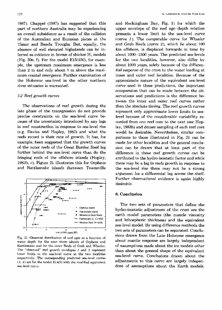
s i o n p r o d u c e d b y t h e m e l t i n g of t h e ice s h e e t s i n

L a t e P l e i s t o c e n e a n d E a r l y H o l o c e n e t i m e . T h e

r e l a t i v e l y c o n s t a n t v a l u e s o v e r t h e p a s t 6000

y e a r s i n d i c a t e s a c e s s a t i o n of m e l t i n g of t h e s e ice

d o m e s b y a b o u t 6000 y r B . P . A s a z e r o - o r d e r

m o d e l of s e a - l e v e l r i s e t h i s is s a t i s f a c t o r y . W h a t

is of g r e a t e r i n t e r e s t a r e t h e d e p a r t u r e s f r o m

t h i s s i m p l e s e a - l e v e l m o d e l . I n p a r t i c u l a r , h a s

144 K. L A M B E C K A N D M. N A K A D A

sea-level been higher than the present value during the Late Holocene? Is there evidence for regional variabili ty in the ampli tude of this emergence? Is there evidence tha t the t ime at which sea-level first reached its modern level varies from one location to another? These are impor tan t questions whose answers are relevant to the s tudy of a number of geophysical and geomorphological phenomena.

The present sea-level signature shows very considerable temporal variability, being driven by oceanographic and meteorological factors, and it is difficult, if not impossible, to recognize secular trends from a few decades of tide gauge records. The longer records provided by geological and geomorphological observations provide valuable indicators of past trends relative to which modern changes can be examined so as to determine possible anthropogenic contributions. For solid-earth geophysics, the global adjustment of the Ea r th to the area distribution of the surface ice and water loads is an example of isostasy at work and it becomes possible to est imate rheological parameters of the Ea r th which in tu rn decide other solid-earth phenomena such as mant le convection. The analysis of sea-level change is also impor tan t for evaluating vertical tectonic processes. Sea-level is the natural da tum relative to which vertical tectonic movements are measured and it is necessary to know how this surface may move in order to decipher recent tectonics. How much, if any, of the spatial variat ion in the Late Holocene highstands is a consequence of tectonics and how much is a consequence of the Ear th ' s response to the change in surface load? For glaciology, the Holocene sea-level curves provide constraints on models of the disintegration of the last great ice sheets. To what extent does the Late Holocene sea-level constrain the melting models of Laurentia, Fennoscandia, and Antarct ica over the past 10,000 years? For geomorphology, the knowledge of sea-level change is impor tan t for understanding coastal response to change in this level. Are regional variations in the late Holocene highstands indicative of a modification or redistr ibution of the intensities of coastal processes through t ime?

The pioneering work on Late Holocene sea- levels in Australia was by R.W. Fairbridge who ident i f ied h ighs t ands along the Wes te rn Australian coastline and who established a sea- level curve tha t was distinctly different from the curves established from nor thern hemisphere data (Fairbridge, 1954, 1961). His sea-level curve first reached the present level a t about 6000 years ago whereas the nor thern European sea- level curves reached their modern values much more recently (e.g. Jelgersma, 1961). Fairbridge's highstands of several metres between 6000 years ago and the present also were not recognized in the European and Nor th American data. How- ever, agreement on Fairbridge's curve was not universal, even within the Australian region. Hails (1965), for example, concluded tha t there was no clear evidence for higher than present Late Holocene sea-levels in eastern Australian (see also Th o m et al., 1969, 1872) whereas Hop- ley (1970) and Gill and Hopley (1972) presented evidence for Holocene highstands alond the Nor th Queensland coast.

Because of careful work by a number of geo- morphologists in the past decade a dist inct pattern of the Late Holocene sea-level variat ion along the Australian coastline is now emerging. In north Queensland estimates of the maximum Holocene emergence range from jus t above the present level to more than 2 m above this level (e.g. Chappell et al., 1983) and in South Australia estimates range from near zero to more than 3 m (e.g. Hails et al., 1983). Much of the evidence is reviewed in the papers edited by Hopley (1983a) and in the reviews by Chappell (1987) and Hop- ley (1987). Sites discussed in the text are illustrated in Fig. 1. The reali ty of the existence of the Late Holocene highstands and of the regional variabili ty of the ampli tudes of the emergence is now widely accepted bu t there is less agreement on the reason for this variability. Is it tectonic in origin or is it the result of the regional variat ion in the Ear th ' s response to the loading of the crust by the mel t -water released from the Late Pleistocene ice s h e e t s - - t h e so- called hydro-isostatic effect? Proponents of bo th views can still be found despite the very con- vincing evidence presented by Chappell et al.

LATE PLEISTOCENE AND HOLOCENE SEA-LEVEL CHANGE ALONG AUSTRALIAN COAST 145

Sound

Tirnor Sea

xmouth G.

Western .~.e,, Australia

Pool

~ aMton

Rottnest Is. =~Per th Geographe Bay

Aug ust a"~",,.~

Arafura Sea

( " ~ L lul l of tam _h'J'M'~ South Carpentaria

I t / ~ ~ ' ~ Alligator ~ ] F ~ ) f i t - ' orningtor' o~ Rwer Sir George ~ Island _ Peilew Group :"'x, O

Ord River

York

Cape Direction ! ~ ~ -Princess Charlotte Bay

Cape Flattery

&[Yule Point Rockingham B. ~Caims 18o,

Yownsville S

Northern "~-~ae,ay Territory "~ ̂ Shoa, ~ate, ~.

Queensland -~]X- ~ s ° s

I Gladstone'~ Fraser Island

South t . . . . Lo,d Coast

i Australia ~ . . . . . - ~ - ~ ' ,~ I New South /Nambu,~a.eads

_Po.Au0Ts~ Wales / ~" ~ / ~ ~ ' ~Hawkesbury R • . ~,/'. Iwallaro~ .,,, ~ • w I Spencer Gult . . . . ~ _ ~ Adelai(:l e " ~ . /Sydney

CapeSpencer' ' i~l~:("'~ [ . r . ?~ 'w' -"- -~ ( ' ' . ' " , I v i c t o r i a \ f Moruya

/ ~,~i Mel_bourne ~ , , ~ t ' Melbourne ~" C Kangaroo Is. / ape Howe Kangaroo Is./;l'"arrna M ~ P ~ ~ w mooor ~ /' "~"..,. ~ Cape Howe

// ~ I WllSOn's ;"rom 2- " I Bumie ~

. J Tasrnania , " ~ ~ ' t [ ~= bwansea C3 "~ "~...J Hobart

g ~ trY0

Fig. 1. Locality map of sites cited in text for which sea-levels have been either predicted or observed.

(1982) that hydro-isostasy was the essential factor in producing spatial variations in the amplitude of Late Holocene highstands in northern Queensland. These authors demonstrated that because of the irregular shape of coastlines and because of the existence of shallow coastal shelves such that shorelines some 10,000 years ago and earlier were much displaced from their present position, the loading of the sea floor by the rising sea during the post-glacial marine transgression is regionally quite variable and capable of producing different highstand amplitudes.

The notion of hydro-isostasy goes back at least to G.K. Gilbert in 1890 in the context of the warping of shorelines of periglacial Lake

Bonneville in Utah, and to the work of Daly (1925). Bloom (1967) revived the hypothesis and quantitative models were developed by Walcott (1972), Chappell (1974a), and Chathles (1975). Farrell and Clark (1976) provided the essential formulation for a global integrated glacio- hydro-isostatic model and most subsequent work has been based on their approach (Peltier and Andrews, 1976; Clark et al., 1978; Nakiboglu et al., 1983). However, none of these global models had adequate spatial resolution for detailed mapping of the warping of shorelines produced at sites far from the ice sheets by the water loading and only Chappell et al.'s (1982) regional model achieved this (see also Chappell, 1974a). But these latter models cannot readily accom-

146 K. LAMBECK AND M. NAKADA

modate the glacio-isostatic contributions which are not negligible at locations as far from the former ice sheets as Australia. Nor can these regional models readily meet the requirement that the sea-surface remains an equipotential surface at all times. These limitations led Nakada and Lambeck (1987) to develop very high spatial resolution global models, based on the Farrell and Clark formulation, which appears to be largely adequate for modelling warping of coastlines over distance as little as 100 km.

In this paper the glacio-hydro-isostatic factors contributing to the spatial and temporal variability of sea-level change ar estabilished for the Australian region and compared with the observational evidence, particularly for the late phase of the post-glacial marine transgression and the Late Holocene emergence. By using differential methods these comparisons permit critical parameters to be established for both the Earth's response to the change in surface load of ice and water, and for the gross char- acteristics of the model for the volume and time of the addition of meltwater into the oceans.

2. Model predict ions

2.1 The glacio-hydro-isostatic sea-level model

The shape of the ocean surface is, in the absence of meteorological forcing, determined by the Earths' gravitational potential and is, therefore, a function of the mass distribution within the solid planet, the oceans and ice sheets. As the ice sheets wax and wane and sea-levels fall and rise in harmony, the gravitational potential is time dependent. Even for a rigid earth the combined attraction of the ice sheets and redis- tributed meltwater can produce a complex spatial pattern of sea-level change. For the real earth this pattern is compounded by the planet's tendency to deform under a redistribution of the surface ice and water loads: flow is induced in the mantle, the mass distribution and gravitational potential become time dependent, and the ocean surface adjusts further to this new gravity field.

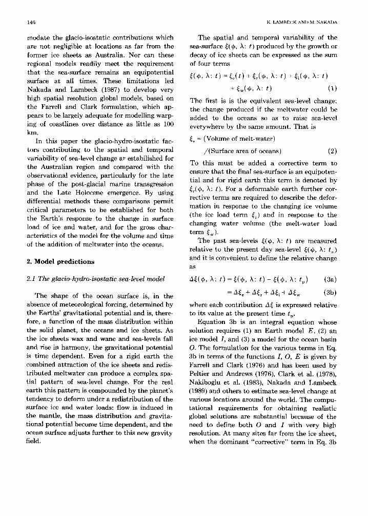
The spatial and temporal variability of the sea-surface ~(~, h: t) produced by the growth or decay of ice sheets can be expressed as the sum of four terms

~(q), h: t ) = ~ e ( t ) + ~ r ( ~ , X: t )+~i(q) , X: t)

+~w(¢, h: t) (1)

The first is is the equivalent sea-level change; the change produced if the meltwater could be added to the oceans so as to raise sea-level everywhere by the same amount. That is

~e = (Volume of melt-water)

/ (Surface area of oceans) (2)

To this must be added a corrective term to ensure that the final sea-surface is an equipotential and for rigid earth this term is denoted by ~r(6, 2~: t). For a deformable earth further corrective terms are required to describe the deformation in response to the changing ice volume (the ice load term ~i ) and in response to the changing water volume (the melt-water load term ~w)-

The past sea-levels 4(0, X: t) are measured relative to the present day sea-level ~(~, h: t . ) and it is convenient to define the relative change a s

3~(0, h: t ) = ~(~, h: t ) - ~(~, h: tp) (3a)

where each contribution A~ is expressed relative to its value at the present time tp.

Equation 3b is an integral equation whose solution requires (1) an Earth model E, (2) an ice model I, and (3) a model for the ocean basin O. The formulation for the various terms in Eq. 3b in terms of the functions I, O, E is given by Farrell and Clark (1976) and has been used by Peltier and Andrews (1976), Clark et al. (1978), Nakiboglu et al. (1983), Nakada and Lambeck (1989) and others to estimate sea-level change at various locations around the world. The compu- tational requirements for obtaining realistic global solutions are substantial because of the need to define both O and I with very high resolution. At many sites far from the ice sheet, when the dominant "corrective" term in Eq. 3b


is the water load, O must be defined with a wavelength of a few tens of kilometres in order to predict the late Holocene sea-levels with ac- curacies better than a metre (Nakada and Lambeck, 1987).

Of the functions required to solve Eq. 3b I and E are poorly known and have to be estimated from the inversion of the sea-level equation. For sites far from the former ice sheet, the sea-level change is insensitive to the details of the melting of the ice and the unknown parameters here are essentially the timing and rates of the addition of meltwater into the oceans; that is, the A}e term in Eq. 3b. Because the relative importance of the corrective load terms (3}i, A}w ) varies with position and time some separation of the Earth and melt-water parameters is possible (Nakada and Lambeck, 1989).

The earth models adopted comprise a high viscosity lithosphere (10 zs Pa s) of thickness Hi, a two layered visco-elastic mantle, and an in- viscid core. The upper-lower mantle interface is defined by the 670 km seismic discontinuity (at depth //670) with an upper mantle viscosity 'Jura greater than or equal to the lower mantle viscosity 'hm. The four model parameters (HI, H~70,

.... ~lm) are effective parameters only and considerable tradeoff between them will be possible. Lateral variations in these parameters are not considered at this stage. Table 1 summarizes the models discussed in the text. Previous work (Nakada and Lambeck, 1989) indicated that likely parameters fall within this range.

The ocean geometry is defined globally with a 10' spatial resolution and its time dependence is represented by a simple three-step function based on the equivalent sea-level function }~ (see fig. 2 of Lambeck, 1990). At times prior to 14,000 yr B.P. the margin is assumed to have occurred at 100 m depth below modern sea-level; between 10,000 and 14,000 yr B.P. the shoreline is assumed to correspond to the present 50-m depth contour and from 10,000 years ago to the present the modern shoreline is adopted. The post-glacial marine transgression around the Australian region is relatively constant and tests with more complex models have indicated that this three-step model is adequate far from the

TABLE 1

Definition of mantle models used in forward modelling of sea-level change. For example, model El4 corresponds to an upper mantle viscosity of 2 x 102° Pa s and a lower mantle viscosity of 1022 Pa s. The models are further defined in the text by the lithospheric thickness. For example, El4(100) corresponds to the above viscosities and to a lithospheric thickness of 100 km.

Im ~ um (Pa S) (Pa s)

1020 2 x 1020 5 x 102') 1021

1021 E1 E2 E3 E4 2 X 1021 E5 E6 E7 E8 5 X 102l E9 El0 E l l El2 1022 El3 El4 El5 El6 2 x 10 22 El7 El8 El9 E20 5 >< 10 22 E21 E22 E23 E24 1023 E25 E26 E27 E28

ice sheets where the zero order term ~e provides a satisfactory approximation of the sea-level curve.

The time scale used throughout is the con- ventional radiocarbon time scale because the observations constraining the ice models as well as the sea-level observations are all expressed relative to this scale.

2.2 Las t Glacial m a x i m u m low sea-level

Observations of sea-level change prior to about 20,000 yr B.P. are sparse and contradic- tory and have not provided high resolution constraints on the fluctuations in ice sheet volume prior to the last glacial maximum at about 18,000-20,000 yr B.P. The position of sea-level at the time of the last glacial maximum has, however, been established at a number of sites in the Australian region at between 130 and 150 m below the present level (Hopley and Thorn, 1983; Chappell, 1987). Lower values for this level, of 80-100 m, are sometimes quoted for northern hemisphere localities (e.g. Johnson and Andrews, 1986) but these sites lie relatively near the margins of the Late Pleistocene ice sheets and the values may not be representative of the equivalent sea-level rise or of ice volumes (Chap- pell, 1974b; Lambeck, 1990). The adopted ice

148 K. LAMBECK AND M. N A K A D A

model ARC3 + ANT3 contains enough ice to raise sea-level on average by 130 m from the onset of deglaciation at 18,000 yr B.P. to the present, consistent with the Australian evidence (Nakada and Lambeck, 1988b).

An important aspect of the last glacial maximum sea-level is that it is not everywhere at the same depth below present sea-level for the rea- sons that underlie Eq. 3b. Figure 2 illustrates some typical predictions for two sections across the Australian margin. The first section (Fig. 2a, c) is along latitude 23.5°S across the Queens- land shelf (see Fig. 1 for location sketch). The second section (Fig. 2b, d) is at longitude 124 °E across the Arafura shelf of northwestern Australia. The ice A~ i and rigid A~ r terms are nearly constant over the Australian region and reflect largely the global change in the gravita-

tional potential produced by the new mass dis- tributions. The regional variation predicted here results from the dependence of the water load term A~w on ocean geometry and on the distance from the coastline. The seafloor is loaded whereas the emerged continent is not and a tilting of the lithosphere is induced across the continent-ocean interface. The predicted 18,000 year old sea-levels are functions of the distance of the locations from the current shoreline as well as of the choice of earth model, of both lithospheric thickness H l and mantle viscosity, and considerable regional variability is predicted. Observational estimates of this depth are, therefore, not unequivocal estimates of the total volumes of the Late Pleistocene ice sheets unless they are interpreted in conjunction with the global glacio-hydro-isostatic sea-level models.

0...

>, o o

g

-110

-120

-130

-140

-150 150

i i i i

& & E1 (50)

v & v . . . . 4150)

"",. ~ ' ~ l ~ E14(50) "",,,N.~ - - * - e25(5o)

" " " \~L~,,~ "'*. . . . . . . . . E27(50)

" " . . . . s

North Queensland latitude 23.5 S

I I , I , l ,

151 152 153 154

110

~20

130

-140

155 -150 -17

b

i , i • i • i • i • i

= Eq50) ~ '~ ~ E4(50)

= E14(50) ~ . . . . "P'" E25(50)

Arafura Sea - /~ longitude 124 E vA&V

, I i I i i i i

-16 -15 -14 -13 -12 -11 -10

-110 m

:~ -120 g g

-13o

-14o

-150 150

C

i i i i

= E14(50)

. . ~ - - = ' - E14(150)

~ "~-.~

North Queensland latitude 23.5 S

= I = I = I * I

151 152 153 154

longitude (degrees east)

-110

-120

-130

-140

' -150 155 -17 -10

d

i i i i i i

E14(50)

. . . . E14(150)

<

Arafura Sea longitude 124 E

i i , i i i i i

-16 -15 -14 -13 -12 -11

l a t i tude (degrees )

Fig. 2. Predicted depths along two sections across the Australian continental margin, a, c. The Queensland shelf at latitude 23.5°S (see Fig. 1) includes the site (V & V) of Veeh and Veevers (1970), b, d. The Timor-Arafura line at longitude 124°E includes the site (vA & V) of Van Andel and Veevers (1967). a, b. These are for a number of different earth models (see Table 1) with H l = 50 km. c, d. These illustrate the predictions for the earth models El4 with lithospheric thickness values of 50 and 150 kin.


2.3 The Postglacial marine transgression

Evidence for sea-level change during the early stages of the post-glacial marine transgression is sparse, presumably because of the rapid rise of level t ha t occurred at this t ime and because the evidence lies a t a depth tha t is generally beyond ready examination. The evidence for the interval from about 10,000-6000 yr B.P. is more plentiful but, at least in the Australian region, not very accurate. The predicted post-glacial marine transgressions from 18,000 to 6000 yr B.P. are i l lustrated in Fig. 3 for sites along the eastern Australian margin from Cape York to Hobart . All sites in Fig. 3a are for coastal positions corresponding to present coastal lake and estuarine environments. Lit t le spatial variation occurs in these predictions, part icularly for the period 10,000-600 yr B.P. for which most observational evidence is available. The exception occurs for Cape York where the sea-level curve closely approximates the equivalent sea-level rise (e.s.1.). Also, little variation occurs for different ear th model parameter (Fig. 3b) and this par t of the sea-level curve is largely independent of the choice of ear th model. Somewhat greater varia- t ion occurs with distance from the shore, primarily because of the tilting effect of the water load term A~ w. In particular, the offshore sea- level curves appear to lag behind the coastal curves by about 1000 years (Fig. 3c) with the

magnitude of this shift being a function of the Ear th ' s rheology. This variat ion will be impor tan t when comparing coastal evidence, generally in the form of mangrove remains or sediment facies changes, with coral growth rate evidence from offshore reefs because the observational bounds on the sea-level envelope may be widened in par t because of this change in the Ear th ' s response across the shelf.

The results of Fig. 3 indicate tha t the dominant contribution to the the far-field sea-level change during the transgression is the equivalent sea-level te rm A~ e and tha t the other contributions can be considered as model dependent corrections tha t can be established with reasonable reliability. Hence, these far-field da ta are sensitive indicators of the t iming and rates at which mel twater is added into the oceans and serve the impor tan t function of constraining the equivalent sea-level curve.

2.4 The time of first attainment of modern sea- level

The Australian data point to sea-level having reached its modern level before about 6000 yr B.P., in contrast to the much later a t t a inment recorded in nor thern Europe and Nor th America. This global variat ion is a direct consequence of the difference in the importance of the ice load term A~i for the two regions; one far from the ice sheet where A~i is small, the o ther near the

~ -50

_~ -I00

-150 -20

. . . . i . . . . i • • •

-.----,e---- Cape York , l ~

I Townsville 1 Gold Coast

Moruya ~ r ~ ..._=_.. Hobart

. . . . i . . . . i , . ,

-15 -10 time (xl000 years BP)

-50

-50

. . . . i . . . . i • • •

---e.--- 51(50) 54(50)

, E14(50)

. . . . i . . . . i , , ,


-100

-150 -100 -20

b c

• i • i -

7 / / " • 152.25 , / ~ " • I 152.67 f ~ 153.O • • 153.5

154.0 i 1 i I i

-12 -10 -8 -6

time (xlO00 years BP)

Fig. 3. Predicted post-glacial mar ine t ransgression from 18,000 to 6000 yr B.P. along the eas te rn margin of Austral ia. a. For different localities and model E14(50). T he dashed line refers to the equivalent sea-level model, b. For Moruya and different ea r th models with H l = 50 km. c. For localities across the Queens land shelf a t la t i tude 23.5°S for model E14(50). Longi tude 151°E corresponds to the present shoreline and longitude 152.25 ° E corresponds to t he Capricorn Group (note different scale).

1 5 0 K . L A M B E C K A N D M . N A K A D A

former ice sheet margin where 5~i represents the dominan t contr ibut ion to relative sea-level change. Within the Austral ian region considerable var ia t ion in the t iming of this event t* has also been recorded. In par t this m a y reflect the imperfect na ture of m a n y of the sea-level indicators (of delays in the response of reef growth to sea-level change, for example) but the predic- t ions indicate t h a t it m a y also be due to the regional var ia t ion in the water load te rm A~,. The adopted equivalent sea-level curve reaches present sea-level a t 6000 yr B.P. but, depending on the magni tudes and signs of the corrective t e rms (A~,, A~i , A~,) , the predicted sea-levels for a deformable ear th m a y reach their present values ei ther af ter or before this nominal da ta of 6000 yr B.P. Far f rom the ice sheet along con- t inental margins IA~w I will generally exceed I A~i ] and l a i r I during the late Holocene. Also, I / ~ [ in this interval is generally positive so t h a t t* > 6000 yr B.P.

Figure 4 i l lustrates schematical ly how the rel- a t ive shift occurs between crust and ocean level along a continental margin. In an interval t~- t 2

sea-level rises rapidly such t ha t the dominant

contr ibut ion to the change is f rom the equivalent sea-level rise A~ . At t ime t 2 mel t ing ceases and thereaf te r A~e = 0 but in this interval f rom t 2 to the present t 3 the sea floor of the deformable ear th is depressed by an amoun t t h a t is a function of t ime and the dis tr ibut ion of meltwater about the site. The water load is t rans- mi t ted via the l i thosphere to the mantle , induc- ing flow away from the sub-ocean man t l e to beneath the unloaded continent, and sea-level appears to fall relative to the crust, even though no water is being extracted from the oceans. The coast itself subsides under the adjacent wa te r load, but by a lesser amoun t than occurs for the open ocean, leaving behind a coastal h ighs tand tha t marks the t ime at which me l twa te r ceased to be added into the oceans. The ampl i tude of this La te Holocene highstand is a function of ear th model pa ramete r s as well as of the position of the site relat ive to the shoreline and of the shoreline geometry. At sites well inland, along a narrow gulf or a deeply indented t idal river estuary, the crustal subsidence is reducd leaving behind a more elevated h ighs tand and an earlier t*.

~ B t 2

~ "" ~ = ~ " ~ . . final sea-level t Rise in

... ., ~,~: : equivalent ~ t) sea-level

relative change "--~_ in sea-level ~ ± deformation of

~ A r crust

t 2

i . . . . . .

~ 3

tl=

t 1 T i m e

~ -//~" t3

t l T i m e ~

Fig. 4. Schematic illustration of sea-level change relative to the crust (a) along a continental margin and (b) at a small mid-ocean island. At time t 1 sea-level begins to rise rapidly up to time t 2 and the shore llines moves from A to B. When no further meltwater is added into the ocean the contributions to further sea-level are the consequence of the Ear th ' s deformation. Under the weight of the additional meltwater the sea floor subsides and the sea-level appears to fall relative to the shoreline to a point C at time t:~. The resulting sea-level curve has the characteristic highstand at the time t 2. At a very small ocean island the island will move with the sea floor and no differential change occurs in interval from t 2 to t:~.

I~a.TE P L E I S T O C E N E AND HOLOCENE SEA-LEVEL CHANGE ALONG AUSTRALIAN COAST 151

For a small ocean island the added mel twa te r loads the sea-floor uniformly and the island subsides with the ocean floor and no relative dis- p lacement occurs and highstands do not develop. Here sea-level reaches its present level when melt ing ceases and then remains a t this level thereafter . This would be the case, for example, for a reef at considerable distance offshore. For large islands some mant le flow will occur from benea th the ocean l i thosphere to the mant le beneath the island, resulting in some differential movements between the island and sea-level such t ha t the Late Holocene sea-level curve resembles a continental margin signal (Nakada, 1986).

The effect of the water load te rm is fur ther i l lustrated in Fig. 5 for the section across the Nor th Queensland shelf outwards from Towns- ville where the predicted t ime t* a t which sea- level first reached its present value increases progressively f rom the outer shelf to the coastline. Other predictions are i l lustrated for sites along Spencer Gulf in South Austral ia where t* increases from the entrance of the gulf to its nor thern end by about 500-1000 yr. Likewise, t* increases with distance inland along tidal estuaries. The var ia t ion in t* predicted along the Austral ian shore is a function of several factors: of the water load A~w, of the ice load if Antarct ic melt ing has been impor t an t in early

Holocene time, and in any La te Holocene ad- j u s tmen t of the equivalent sea-level curve. In models in which no mel twa te r is added af ter 600 yr B.P. (Fig. 5), the change in t* with distance f rom the coastline is abou t 1000 yr and rela- t ively independent of the choice of mant le viscosity, bu t in models in which mel twa te r con- t inues to be added into the ocean af ter 6000 yr B.P. (see below) the var ia t ion in t* with distance f rom the shoreline is much more significant and observat ions of this quant i ty m a y be impor tan t in constraining Late Holocene mel t models.

2.5 Late Holocene sea-level highstands

Figure 4 i l lustrates qual i ta t ively how Late Holocene highstands can develop along con- t inental margins because of the ad jus tmen t of the E a r t h to the water load added a t an earlier time. But the ice load t e rm is not wholly insig- nificant. Figure 6 i l lustrates 5~i a t t = 6000 yr B.P. for sites along the eastern margin from southern New South Wales to Cape York. The Arctic contr ibut ion to A~ i is essentially constant for these sites bu t the Antarct ic contr ibution exhibits a la t i tude dependence, indicating t ha t the Austral ian sea-levels are not entirely independent of the source region for the melt-water . Also i l lustrated is the water load te rm A~ w

-4

t*

-6.0

,F o"

q)

Queensland shelf near TownsvUle i | t I i I l

0 100 200

distance (krn)

-6.5

Section along Spencer Gulf ,,,,* ~ i f ' ¢t~

o" oj

n3 ," ~ (..)

/

-8 -7.0 , i , i . i . I , l , I , m •

-100 300 -50 0 50 "i 00 150 200 250 300 350

b distance (km)

Fig. 5. The time t* at which sea-level first reached its present value predicted for the model E14(50) for (a) a section across the North Queensland shelf at 18°S and (b) along Spencer Gulf from Port Augusta to Cape Spencer. The solid line is for the ice model ARC3 + ANT3 in which all melting ceased at 6000 yr B.P. The dashed line is for a modified ice model in which minor Antarctic melting continued from 6000 yr B.P. to the present (see below).


o

-I

a

A R C 3

-r-

o . o >- ~. ° . ° -

°

.° ° • •

i I i I i I

-40 -30 -20 -10 latitude

i i

o ARC 3 ..',, ,,, ~ ' ~,.--t ~ 0 . . ° , ~ ; , , ~ ~ .¶

: '~ : ", O : ', o

." A N T 3 ..@. ', " o" ', . . .o "~' ',,0 : # ' - e . . . . . o ' " ' " : g • " , , J , "

I .'m ¢ " b, ~- • o" • •

o =~,~ ~ , ~ , -40 -30 -20 - 1 o

latitude

Fig. 6. The predicted corrective terms ~ i , ~ w for sites along the eastern margin of Australian from Cape Howe to Cape York for the ARC3 and ANT3 ice models, and for the earth model E14(50) at 6000 yr B.P.a. The ice load term ~ i ; b. The water load term A~ w.

whose amplitude can vary quite rapidly from site to site in accordance with changes in coastal geometry by amounts that tend to mask the latitudinal dependence of A~ i. The predictions do exhibit a small latitude dependence along the eastern margin, with generally increasing highstands from south to north. The ratio of the water load terms from the Arctic and Antarctic ice sheets is very nearly constant and equal to the ratio of the corresponding equivalent sea- level contributions, confirming that the water load term is independent of the source region of the melt-water in the Australian region.

Figure 7 illustrates the predicted water load term A~w (Fig. 7a) as well as the total A~ (Fig. 7c) along a section across the Queensland shelf

at 23.5 ° south latitude. The other two terms, with A~ i being constant to a high degree of approximation, are illustrated in Fig. 7b. Well- developed highstands are predicted at the present shoreline (longitude 151 ° ) whereas offshore the predicted highstands are much reduced. Other than being rheology dependent, the A~ W term contributing to the Holocene highstand is also a function of the shifting of the shoreline as the transgression proceeds prior to 6000 yr B.P., enhancing the coastal highstands because the localities at which the highstands are now pre- served were initially further inland. The highstands are also a function of the equivalent sea- level curve (see below) and if the equivalent sea-level change is not zero in the past 6000

i • i • i • i i i

0 ~ 0 0 4 151 --t / I ~ 151 , 152.25 / I • 152.25 • 152.67

equivalent sea-level ~ ; 152.67 • 11. 153 ~ o 153

153.5 | 153.5

154 154 - 5 , i . , . , . - 5 i i i - 5 i . , . , .

-8 -6 -4 -2 -8 -6 -4 -2 -8 -6 -4 -2

a b time (xlO00 years BP) C

Fig. 7. a. Predicted water load term /l~w across the Queensland Shelf at 23.5°S, for earth model E14(50) and ice model ARC3 only. Longitude 151°E corresponds to the present shoreline, b. Ice load term A~i , and the equivalent sea-level /~e for the nominal equivalent sea-level model in which all melting has ceased by 6000 yr B.P.c. The relative sea-level change across the shelf.

L A T E P L E I S T O C E N E A N D H O L O C E N E S E A - L E V E L C H A N G E A L O N G A U S T R A L I A N C O A S T 153

2.o~ " R;ckingham Bay "

1 . 5 ~ - E 1 4

o . , ~ ] iif ,'E', i

-6 -4 -2 0

2.0 "'''"0 E16' Rockingh;m Bay 1.5 ~ , ~ " " 0 .

1.0~ E 1 4 " ' ' " o .

-0.5 , I , I , ~6 -4 -2

b

4 i i

Karumba

3

2 E2

6 -4 -2 d

4 • i i

3t." Karumba

f . . . . ' - ~ , ~ . o . .

~6 -4 -2 0

1.5 ' l ' ' i •

ape Spencer

0.5

_0,5 I ~ I , I -6 -4 -2

e

i i

Port Augusta

E4 2 E2 t

. . . .

-6 -4 -2 t ime ( x lO00 years BP)

1.5 • i • i •

~:z--,...~_ 2 ~

-0.5 I , I ~ I , -6 -4 -2

5

0 -6

i • i

• , Port Augusta

-4 -2

time (x1000 years BP)

Fig. 8. Predicted contributions to Late Holocene sea-levels at North Queensland (Rockingham Bay and Karumba) and Spencers Gulf (Cape Spencer and Port Augusta) localities from ice load (left hand side) and water load (right hand side). The predictions are for four Earth models all with H i = 50 kin. Models E2, E 4 are characterized by low values for lower mantle viscosity (~h~l) and models E 1 4 and E 1 6 are characterized by high ~lm.

154

years then the Late Holocene emergence is di- rectly modified. The water load term 5~w is however insensitive to small changes in the equivalent sea-level curve.

The water and ice load terms for Late Holo- cene time are illustrated in Fig. 8 for four sites and for different mantle models (all with H l - 50 kin). At all s i tes/~w > A ~ i and the ice load term is relatively constant for any given earth model (compare, for example, the A~i predictions for each model El4 in Fig. 8a, c, e, g). The amplitudes of these contributions are, however, strongly earth-model dependent, primarily on lower mantle viscosity ~l~. Models E2 and E4, which differ in upper mantle viscosity ~um, produce distinctly different amplitudes than the high valued ~l~ models (El4, El6). The dependence of the water load term on the choice of mantle model is more complex and is a function of position as well. The predictions for the Rockingham Bay site (Fig. 8a, b) are characteristic of most localities along the eastern Australian margin where deeply indented bays and gulfs do not occur. At Karumba (Fig. 8c, d), in the south-east corner of the Gulf of Carpen- taria, the highstand is much enhanced compared to Rockingham Bay because of the distinctly different water loading term produced by the gulf geometry and by the fact that at 10,000 years ago the shoreline was more than 700 km to the northwest of its present position. A similar enhancement is predicted for the northern region of Spencer Gulf (Port Augusta) (Fig. 8g, h).

Other than the amplitude of the highstand another important characteristic of the predicted sea-level curve is the rate of fall of sea-level between 6000 yr B.P. and the present. For models such as El4 and El6 the two terms A~i and 5~w as well as the total sea-level change (the sum of ~ i and A~w ) is predicted to fall nearly uniformly in this interval whereas for models E2 and E4 the predicted fall occurs rapidly after the maximum highstand is attained (Fig. 8). Observations of the sea-level curve after 6000 yr B.P. are therefore as important in constraining mantle models as the maximum amplitude of the emergence itself.

K. L A M B E C K A N D M . N A K A D A

2.6 Differential sea-level change

The relative constancy of the A~i and A~ r term over large areas of the Australian region suggests that the differential sea-levels, defined for sites, m, n as

~ ( m , , . = A,~(m~ _ A d , , ) _ ( , , . (,,) - a ~ w - A ~ w ( 4 )

are largely free of the assumptions made about

f f f f t

4 o

S ~ 3 /111

4

! / C -8 8 4 0

i

4 0

hmelx 1000 years)BP

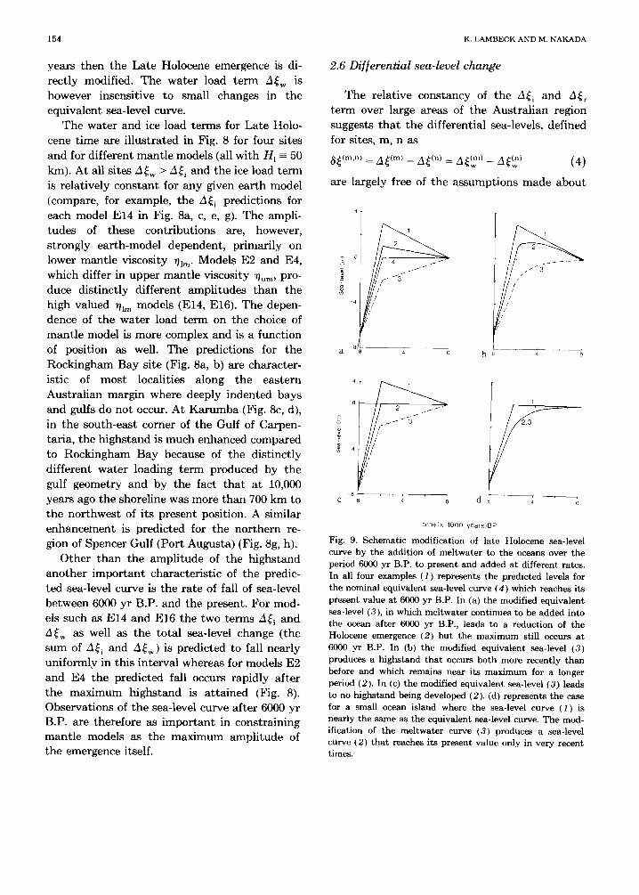
Fig. 9. Schemat ic modif icat ion of late Holocene sea-level curve by the addi t ion of mel twate r to the oceans over the period 6000 yr B.P. to present and added a t different rates. In all four examples (1) represents the predicted levels for the nominal equivalent sea-level curve (4) which reaches its present value a t 6000 yr B.P. In (a) the modified equivalent sea-level (3), in which mel twa te r cont inues to be added into the ocean af ter 6000 yr B.P., leads to a reduct ion of the Holocene emergence (2) bu t the m a x i m u m still occurs a t 6000 yr B.P. In (b) the modified equivalent sea-level (3) produces a h ighs t and t h a t occurs bo th more recent ly t h a n before and which remains near i ts m a x i m u m for a longer period (2). In (c) the modified equivalent sea-level (3) leads to no h ighs tand being developed (2). (d) represents the case for a small ocean island where t he sea-level curve (1) is nearly the same as the equivalent sea-level curve. T h e modification of the mel twa te r curve (3) produces a sea-level curve (2) t h a t reaches i ts present value only in very recent t imes.

L A T E P L E I S T O C E N E A N D H O L O C E N E S E A - L E V E L C H A N G E A L O N G A U S T R A L I A N C O A S T 1 5 5

the ice models and are dependent only on the assumed equivalent sea-level curve. As noted above, sea-level curves in the Australian region are also a function of the equivalent sea-level curve during the Late Holocene. For example, if glacial melting did not cease at 6000 years ago, bu t continued at a slow rate up to the present, it would have a direct consequence on the Late Holocene sea-level curve: additional mel twater tha t raises equivalent sea-level by 1 m from 6000 years ago to the present lowers the highstands at all sites in the Australian region by about 1 m (Fig. 9). Such a modification also affects the t ime at which the present level first occurs (Fig. 5) but because these Late Glacial mel twater contr ibutions are unlikely to be large, their consequence on sea-levels before about 6000 yr B.P. are generally small. The ambiguity introduced into the interpreta t ion of the highstands by this additional unknown is largely removed if the

23

E 22

21 a 20 2~

H=50 km

O ~ 22

b 28 2t H=50 km

Karumba - Rock lngham Bay

2O 21

H=tO0 km

\~ 1,7~ =

--...--.~_ 20 21

P1=150 km

Port Augus ta - Cape Spencer

20 21 H~IO0 km

log i 1 urn

/ \ 2.5

1

20 21

H=150 km

Fig. 10. Differential highstands as a function of upper and lower mantle viscosity and lithospheric thickness H i for (a) Karumba and Rockingham Bay, North Queensland, (b) Port Augusta and Cape Spencer, Spencer Gulf, South Australia. The shaded areas define the acceptable solution space defined by the observations of differential sea-level in those two regions.

differential sea-levels (4) are used. For example, the predicted difference in highstand ampli tudes between Karumba and Rockingham Bay is largely independent of such adjus tments of the dis tant ice sheets, including small equivalent sea-level changes in La te Holocene time, and these differences constrain well the mantle models. Once opt imum mant le models are established from comparisons of predicted and observed differential sea-levels defined by (4), the amplitudes of the highstands can be used to determine whether ad jus tment of the equivalent sea-level curve is warranted. Figure 10 illustrates the differential highstands for the two nor thern Queensland sites of Karumba and Rockingham as a function of upper (~u~,) and lower (~lm) mantle viscosity and for three different H l values. Also i l lustrated are the predictions for two South Australian sites, Por t Augusta and Cape Spencer. Both examples i l lustrate the complex dependence of the differential high- s tand amplitudes on upper and lower mant le viscosity and the lesser dependence on lithospheric thickness.

3. C o m p a r i s o n of observations and predictions

3.1 The Las t Glacial m a x i m u m

Observations of sea-level a t the t ime of the last glacial maximum provide constraints on the total volume of the grounded ice sheets t ha t melted af ter about 18,000 yr B.P. (Floating ice sheets do not contr ibute to sea-level change.) Observational evidence from the Austral ian region points to this level having been at between 130 m and 165 m below the present level. This includes submerged beach rock, shallow marine, intert idal or subaerial sediments and organic materials, and shallow water corals t h a t have been dated as being of Late glacial maximum age. Hopley and Th o m (1983) and Chappell (1987) have reviewed the evidence.

Of the predictions i l lustrated in Fig. 2 the Queensland shelf section includes the site examined by Veeh and Veevers (1970). The evidence here includes dated in situ samples of

156 z . LAMBECK A N D M. N A K A D A

shallow water corals and gastropods and indicates that the maximum lowering of sea-level was about 160-165 m although the level could have been several tens of meters higher. For comparison, the model predictions indicate values of between 130-135 m. The second section illustrated in Fig. 2 includes the locality examined by Van Andel and Veevers (1967). The evidence here is a core sample of a change from lagoonal to marine sedimentation which points to sea-level having been at about 130 m during the glacial maximum (see also Jongsma, 1970).

Ice models for the major ice sheets of Laurentia and Fennoscandia contain only a frac- tion of the ice required to produce the sea-level change of this magnitude. Even the maximum reconstruction of Denton and Hughes (1981) for these two ice caps contain only enough ice to raise equivalent sea-level by 110 m yet this model has been criticized for over estimating the ice volume (Andrews et al., 1983; Johnson and Andrews, 1986). Hence additional ice sources are required for explaining the Australian data and this is the reason for including the Barents-Kara ice sheet and an Antarctic contribution in the ice models used in these predictions (Nakada and Lambeck, 1988b; 1989). It must be empha- sized, however, that from this evidence alone

only the volume of additional meltwater and not its source, can be estimated.

3.2 The post glacial marine transgression

Evidence for sea-level change during the marine transgression is sparse and not very accurate. Much of the information is in the form of imprecise indicators such as in situ tree stumps or in situ reef growth or mollusc shells. The tree stump information indicates that sea- level was below the position of the dated material, whereas the coral information indicates that sea-level was somewhere above the dated growth positions. Mangroves, whose growth range corresponds approximately to the tidal range, provide particularly useful constraints on the limits of past sea-level change. Thus what can generally be established is an envelope of sea-level change (Thorn and Chap- pell, 1975; Thom and Roy, 1983).

Figure 11 illustrates the evidence for the New South Wales coast (Thom and Roy, 1983) and for Christchurch (New Zealand) (Gibb, 1986). These data sets represent the most complete information for the latter part of the marine transgression in the Australian region. Both data sets exhibit considerable scatter but both are

o 0 s "

- 2 0 -20 ~ I "

N

" -60 , i | I I i

a - 12 -10 -8 -6 -4 -2 0 -12 -10 -8 -6 -4 -2

time (xlO00 years 8P) b time (xlO00 years BP)

Fig. 11. Observational evidence for the late post-glacial marine transgression (a) along the central and southem coast of New South Wales (Thom and Roy, 1983) and (b) for Christchurch (Gibb, 1986). Predicted sea-levels for these localities are based on the Arctic model, the Antarctic model ANT3, and the combined model ARC3 + ANT3.

LATE P L E I S T O C E N E AND HOLOCENE SEA-LEVEL CHANGE ALONG AUSTRALIAN COAST 157

similar to those observed at other coastal far- field sites such as the Malay Peninsula (Geyh et al., 1979) and Japan (Yonekura and Ota, 1986). Within the measurement and interpretat ion er- rors there is little evidence for regional variation in this part of the sea-level curve at sites far from the former ice sheet margins.

Of importance in comparing these observations with the predictions is tha t the two are inconsistent for models based on the melting of the Laurent ide and Fennoscandian ice sheets only (This is the Model ARC 3 in Fig. 11). Ei ther additional mel twater must be added into the oceans at about the same time as these Arctic contributions (the model ARC 3 + ANT3, Fig. 11) or Arctic melting must be moved forward in time, by about 1500 years, in order to match observations and predictions. Geomor- phological evidence for the Laurent ide and Fen- noscandian ice sheets, as well as the sea-level da ta near these ice centres, precludes the la t ter interpretat ion and, instead, additional ice must be introduced into the late Pleistocene ice sheets (Clark and Lingle, 1979; Nakiboglu et al., 1983; Nakada and Lambeck, 1988b). This is consistent with the evidence for the glacial maximum sea- levels discussed above but it provides the additional requirement tha t this melt-water must have been added relatively recently; at about the same t ime as the bulk of the Laurent ia and Fennoscandia ice sheets between 14,000 and 8000 years ago. Earlier melting, while resolving the glacial maximum sea-level question at 18,000 years ago, do not contr ibute greatly to the marine transgression between 12,000 and 6000 years ago. The conclusion tha t significant contr ibutions to the sea-level rise must have come from the grounded ice in Antarctica seems in- escapable.

Within a good approximation and within observational uncertainty, the predicted transgression is very similar along the Australian coastline and largely insensitive to the choice of mantle model for as long as the equivalent sea-level t e rm A~ e dominates the total sea-level change. Significant variation in the transgression is, however, predicted across continental shelves, the offshore curves lagging behind the coastal

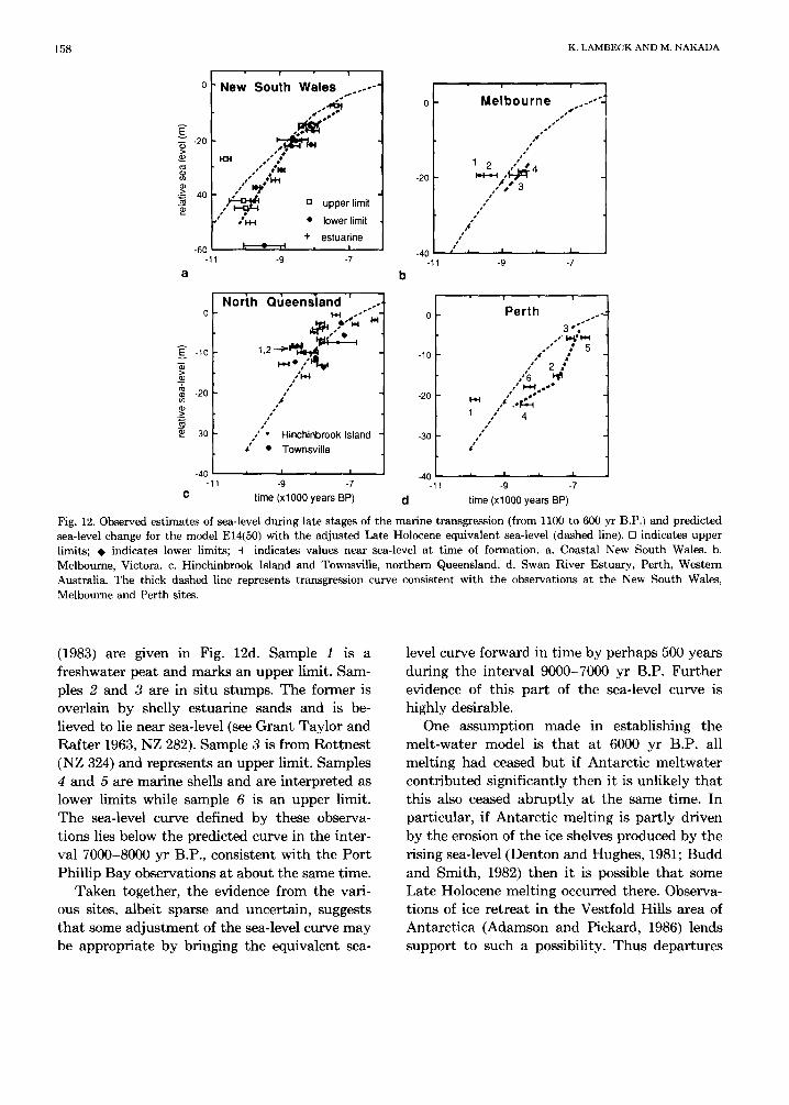
curves by amounts tha t are a function of distance from the coast and a function of ear th parameters (Fig. 3c). The adopted mel twater curve is generally consistent with the available data in the far-field (Fig. 11), including sites beyond Australia, a l though it has been suggested tha t the predicted sea-level rise occurs somewhat earlier than observed in the interval 9000-7000 yr B.P. (Nakada and Lambeck, 1988b). Figure 12a illustrates the observations for New South Wales by Th o m and Roy (1983) for the interval 11,000 to 6000 yr B.P. in which samples defining an upper limit (tree stumps) are separated from those defining a lower limit (marine shells) and from estuarine deposits assumed to lie near sea-level. These samples suggest a sea-level curve tha t lies below the predicted values and tha t some ad jus tment of the equivalent sea-level curve may be warranted in which the equivalent sea-level curve is brought forward by about 500 years in the interval 9000- 7000 yrs B.P.

A few other disparate observations exist for the Australian region. The Melbourne observations (Fig. 12b) (Gill, 1967) comprise wood samples (point 1, 2), an in situ tree s tump (point 3) and freshwater peat (point 4) and these define an upper limit to the sea-level curve. A comparison with the predicted transgression suggests t ha t the rise occurred somewhat earlier than observed (Fig. 12a) and consistent with the New South Wales observations. The Nor th Queens- land observations comprise primarily Rhizo- phora mangroves which inhabit the tidal range between about the mean low and mean high tidal ranges. The observations are from two nearby localities for which the models predict little spatial difference over a wide range of ear th parameters. The Hinchinbrook Island da ta (Grindrod and Rhodes, 1984) includes a non- Rhizophora mangrove and a brackish swamp deposit (points 1, 2, Fig. 12c) which define an upper limit to the sea-level curve at about 8500 yrs B.P. The Townsville observations (Belperio, 1979) are generally consistent with the predicted sea-levels.

A few observations from the Swan River (Perth, Western Australia) reported by Brown

] 5 8 K . L A M B E C K A N D M . N A K A D A

• ! • i

o N e w South Wales , - . . . . .

~ -2(1 ~

N / **m ~ - 4 0 °

gH~

-60 1, e ~ :

-11 -9

a

[] u p p e r l imi t

l o w e r l imi t

+ e s t u a r i n e i i

-7

-20

- 4 0 -11

i i

M e l b o u r n e I : s ~

14 ° s t

s

s ~

J

-g -7

-10

-20 03

~ - 30

-10

Nor th Queens ' land ' . . . ~ " .

1 F2

~°-~h~ eel,~

,,s s

s S lee

• ' ° H i n c h i n b r o o k I s l a n d

,~ • T o w n s v i l l e

-9 -7

t i m e ( x l 0 0 0 y e a r s BP)

- 2 0

- 3 0

i i

Per th

os" ll~mJ I'~1

1 , 4 e I

s S s • 4 t

-40 -40 ; I ~ I -11 -11 -9 -7

C d time (xl000 years BP)

Fig. 12. Observed estimates of sea-level during late stages of the marine transgression (from 1100 to 600 yr B.P.) and predicted sea-level change for the model E14(50) with the adjusted Late Holocene equivalent sea-level (dashed line). [] indicates upper limits; ~ indicates lower limits; + indicates values near sea-level at time of formation, a. Coastal New South Wales. b. Melbourne, Victora. c. Hinchinbrook Island and Townsville, northern Queensland. d. Swan River Estuary, Perth, Western Australia. The thick dashed line represents transgression curve consistent with the observations at the New South Wales, Melbourne and Perth sites.

(1983) are given in Fig. 12d. Sample 1 is a freshwater peat and marks an upper limit. Sam- ples 2 and 3 are in situ stumps. The former is overlain by shelly estuarine sands and is believed to lie near sea-level (see Grant Taylor and Rafter 1963, NZ 282). Sample 3 is from Rot tnes t (NZ 324) and represents an upper limit. Samples 4 and 5 are marine shells and are interpreted as lower l imits while sample 6 is an upper limit. The sea-level curve defined by these observa- t ions lies below the predicted curve in the interval 7000-8000 yr B.P., consistent with the Port Phillip Bay observations at about the same time.

Taken together, the evidence from the various sites, albeit sparse and uncertain, suggests that some adjustment of the sea-level curve m a y be appropriate by bringing the equivalent sea-

level curve forward in t ime by perhaps 500 years during the interval 9000-7000 yr B.P. Further evidence of this part of the sea-level curve is highly desirable.

One assumpt ion made in establishing the mel t -water model is that at 6000 yr B.P. all melt ing had ceased but if Antarct ic mel twater contributed signif icantly then it is unlikely that this also ceased abruptly at the same time. In particular, if Antarct ic melt ing is partly driven by the erosion of the ice shelves produced by the rising sea-level (Denton and Hughes, 1981; Budd and Smith, 1982) then it is possible that some Late Holocene melt ing occurred there. Observa- t ions of ice retreat in the Vestfold Hills area of Antarct ica (Adamson and Pickard, 1986) lends support to such a possibility. Thus departures

L A T E P L E I S T O C E N E AND HOLOCENE SEA-LEVEL CHANGE ALONG AUSTRALIAN COAST 159

from the adopted equivalent sea-level curve can be expected in Late Holocene time. If small, such departures will not modify significantly the per turbat ion terms, particularly A ~ , in Eq. 1, but it will modify the equivalent sea-level te rm A~. The Late Holocene will provide fur ther constraints on the Late Holocene par t of the equivalent sea-level curve because sea-levels in this interval are a function of both this model and of the earth model E.

3.3 Observations of Late Holocene emergence

The best evidence for Holocene highstands is found in nor thern Queensland. Chenier ridges along the shore of the Gulf of Carpentar ia indicate highstands in excess of 2 m having developed by about 6000 yr B.P. (Smart, 1976; Rhodes, 1982) and the ridges near Karumba are particularly significant. Here the highstand is 2.5 m above present level and sea-level dropped at a uniform rate to its present value (Chappell et al., 1982) (see Fig. 13a). To the west, in the Sir George Pellow Group of islands, a highstand of about 1.2 m has been reported by Rhodes (1980). Another impor tan t data set is provided by micro-atalls on the off-shore islands and reefs of north-eastern Queensland. These observations indicate a highstand of about 1.0-1.5 m at about 6000 years ago with the suggestion of some geo- graphic variat ion in this height. For Dunk and Goold Islands in Rockingham Bay, nor th of Townsville, the evidence points to a highstand of about (1.0 _+ 0.3) m in (Fig. 13b) (Chappell et al., 1983). For King and Flinders Islands in Princess Charlot te Bay (Chappell et al., 1983) and for the nearby Howick Group southeast of

Fig. 13. Relative sea-level change (with error bars) observed at (a) Karumba, Gulf of Carpentaria, for past 6000 years, (b) Dunk and Goold Islands in Rockingham Bay, North Queens- land, (c) near Cape Melville, as defined by the observations from King and Flinders Islands and in Princess Charlotte Bay and islands in the nearby Howick Group. The dashed lines represent the model predictions for the optimum earth model and the unadjusted equivalent sea-level model. The continuous lines represent the predictions using the adjusted equivalent sea-level model.

Cape Melville a similar highstand of (1.0 +_ 0.3) m is indicated (McLean et al., 1978) (Fig. 13c). Fur ther north, a t Thursday Island (Cape York), limited micro-atoll da ta suggests t ha t the maxi-

4 E

o 2

o 0

-2

-4 -8

tit, ,~ I I

K a r u m b a Gulf of Carpentar la

, I i I i I i

-6 -4 -2

4 E

o 2

f~9

o 0 .>_

-2

-4 -8

I • I • I •

7 " .

!

Goold & Dunk Islands N o r t h e r n Q u e e n s l a n d

, I , I , l ,

-6 -4 -2 0

A 4!

-$ 2

Q} ( / )

0

-2

-4 -8

C

King & Fl inders Is lands and Howick G r o u p , N o r t h e r n Q u e e n s l a n d ~i' I , I , I ,

-6 -4 -2 0

time (xlO00 years BP)

160

TABLE 2

Summary of observational evidence for emergence at 6000 yr B.P.

Site rsl (m) Reference

Karumba 2.5 + 0.3 Chappell et al., (1983) Sir George Pellow 1.2 ± 0.5 Rhodes (1982) Cape York 0.8 ± 0.5 J. Chappell

(pers. comm., 1989) Cape Melville 1.0 ± 0.3 Chappell et al., (1983);

McLean et al., (1978) Rockingham Bay 1.0 ± 0.3 Chappell et al., (1983) Moruya 0.5 ± 0.5 Thorn and Roy (1983) Port Augusta 3 ± 0.5 Belperio et al., (1984);

Burne (1982) Cape Spencer 0.5 ± 0.5 Belperio, et al., (1983);

Short, et al., {1986) Christchurch (NZ) 0 ± 1 Gibb (1986) Weiti (Hauraki

Gulf, NZ) 0.9 ± 0.5 Gibb (1986)

mum highstand attained was about 0.8-1.0 (J. Chappell, 1989, pers. comm.). Like the Karumba data, the change in sea-level after 6000 yr B.P. seems to have been quite uniform up to the present (Chappell et al., 1983; Chappell, 1987) and where necessary, this trend has been ex- trapolated to produce estimates of sea-level at 6000 yr B.P. to facilitate comparisons with the predictions. Table 2 summarizes the observations used.

A recent observation of an intertidal calcare- ous worm tube of Late Holocene age (Flood and Frankel, 1989) suggests that a well-developed highstand existed along the northern New South Wales coast (Nambucca Heads) reaching an amplitude of at least 1 m. In contrast to these highstands, the central and southern New South Wales coast does not contain evidence for highstands much above the present level, although this level was first reached shortly before 6000 yr B.P. Much of this evidence has been reviewed by Thom and Roy (1983). This includes in situ tree stumps dated at between 3000 and 6000 yr B.P. found at several localities near the present high-water mark. A maximum level of 0.5 + 0.5 m has been adopted for the coastal zone of Moruya. Of potential interest is the apparent absence of a distinctive highstand,

K. LAMBECK AND M. NAKADA

within an observational precision of about + 1 m, up to 50 km inland from the coast along the Hawkesbury River (B.G. Thom, pers. comm., 1989).

In South Australia, well-developed highstands are found at the northern end of Spencer Gulf (Belperio et al., 1984; Hails et al., 1984; Burne, 1982). Here the evidence consists primarily of seagrass banks at heights of 3 m and more above their modern equivalents which grow up to the low water mark. Near the entrance to the gulf, on both the Yorke and southern Eyre Peninsulas, such highstands do not appear to have developed (Belperio et al., 1983; Short and Fotheringham, 1986; Short et al., 1986).

Elsewhere along the Australian coastline the evidence is less clear. The Holocene highstand has not been identified along the coastline of Tasmania (Bowden and Colhoun, 1984). Near Perth, Western Australia, the evidence is con- tradictory. An estimate for the Swan River Estuary suggests an emergence of only 0.5 m (Kendrick, 1977) whereas about 2.5 m has been estimated for Rottnest Island only 20 km away (Playford, 1983). At sites to both the north and south of Perth highstands of 2-3 m have been reported (Woods and Searle, 1983; Searle and Woods, 1986). These higher values are hard to reconcile with the Swan River estimate unless there has been some local tectonic subsidence, or sediment compaction has been important at this latter locality compared with the Rottnest and coastal estimates.

Observations of Holocene emergence in New Zealand have been reported by Gibb (1986) but the interpretation of the data is complicated by the possibility of the occurrence of vertical tectonics. His most complete data set is for the Weiti River Estuary (the Hauraki Gulf of North Island) for which an emergence of 0.9 _+ 0.5 m at 6000 yr B.P. appears appropriate (table 3 of Gibb, 1986). This site is believed to be tectonically stable. For sites near Christchurch and Blueskin (South Island) the evidence suggests that little change in sea-level has occurred during the past 6000 years and a nominal value of 0 ± 1 m at 6000 yr B.P. is adopted for Christchurch.


4. Est imat ion of model parameters

4.1 Earth model parameters

The dependence of the sea-level curve on earth and ice-model parameters discussed in section 2 suggests that an iterative procedure is appropriate for estimating the various unknowns. First an approximate equivalent sea-level curve is established from the Last Glacial maximum

and the marine transgression phase (in this case the ARC3 and ANT3 ice model defined above). With this model the spatial variability of the Late Holocene sea-level is predicted and the predicted differences (4) are compared with the observations to estimate the Earth model E. One E is established the amplitudes of the Ho- locene emergence is used to estimate corrections to the equivalent sea-level curve for the middle and Late Holocene. If these corrections are not

E 22

b 21

Karumba- Cape York

lt2S ~ '

~ t O 21 a 20 21

Rockingham Bay- Cape Melville

23 , , , ,

Karumba- Cape Melville

2.0

1.5

20 21

Karumba- Rockingham Bay

ll 1 \ t = \

1 2 "~'%

Karumba- Pellew Grou

0.f

~0.4. I i I [

20 21

Cape York- Rocklngham Bey

Kerumba- Edward River

20

Rocklngham Bay- Moruya

0.5

5

21

Hauraki- Christchurch

Port Augusta- Cape Spencer

23 3

3.5

22

21

Moruya- Christchurch

I I I I I

20 21 20 21 20 21

Moruya- Haurakl Gulf

20 21

log % m

Fig. 14. Di f fe ren t i a l h i g h s t a n d s as a func t ion of u p p e r l~u m and lower T~[ m mantle viscosity for localities in northern Queensland, N e w S o u t h Wales , S o u t h A u s t r a l i a a n d N e w Z e a l a n d for H 1 = 50 km. The observed spatial differences for each p a i r of sites define the permissible solution spaces indicated by the shading•


small then an iterative procedure can be used to est imate further ref inements to both earth and ice models.

Typical values for the spatial differences are il lustrated in Fig. 10 as a function of upper ~um and lower ~h~ mant le viscosity and l ithospheric thickness H 1. The observed differential highstand for Karumba and Rockingham Bay is 1.5 _+ 0.4 m and this defines a broad range of

upper and lower mantle viscosities that yield predictions consistent with the observed values. The Port Augusta-Cape Spencer differential highstand of 2.5 + 0.7 m provides a further con- straint as do the other pairs of sites illustrated in Figs. 14-16. Any single pair of stations does not generally provide a strong solution for the viscosity but when observations from a number of sites are used the combined data set defines

--" 22

b 21

Karumba- Cape York

.5

22

20 21

Rockingham Say- Cape Melville

23

Karurnba- Cape Melville

20 21

Karurnba- Rockingharn Bay

\,.\

Karumba- Penew Group

I f I j h

,.i. oA I

20 21 20

Cape York- Rockingham Say

Karumba- Edward R.

l

2i

Rockingharn Bay- Moruya

0.5

Port Augusta- Cape Spencer

23

Moruya- Hauraki Gulf

22 3.5

20 21


-1' 1

Hauraki Gulf - Christchurch

20 21 C 20 21 20 21

log qum

Fig. 15. Same as Fig. 14 bu t for H l = 100 km. T h e differences involving Cape Melville point to low values for both upper and lower mant le viscosity (defined by the shaded areas in the lower left hand corners) which are not only inconsis tent wi th the o ther spat ial differences bu t also inconsis tent with the observat ion t h a t sea-levels af ter 6000 yr B.P. drop fairly uni formly to thei r present level.


Karumba- Cape York

23

2t ~ ~ a 20 21

Rockingham Bay- Cape Melville

23

.0

~ - 22

Karumba- Karumba- Cape Melville Pellew Group

3

20 21

Karumba- Rockingham Bay

20 Ill

21

Cape York- Rocklngham Bay

~ o . s 10.75

/ Port Augusta- Cape Spencer

C 20 21

Fig. 16. S a m e as Fig. 15 but for H = 150 k m


20 21

Hauraki- Christchurch

20 21

log q um

Karumba- Edward River

1.51

1.5

20 21

Rockingham Bay- Moruya

Moruya- Hauraki Gulf

0

0.5

1.5

20 21

narrow limits on these mant le parameters. The search for model parameters is restricted to the range (10 ~t) < ~um < 1021) Pa s, (1021 < 7~1 m < 102~) Pa s, and H l = 50, 100, 150, 200 km because earlier results have indicated that this range encompasses the likely solution space (Nakada and Lambeck, 1989; Lambeck, 1990).

A formal inversion of the model is not at- tempted and a forward model l ing procedure has been adopted in which acceptable solution spaces are sought for each of the discrete values of H I. Acceptable is defined here as the ~um -- ~lm space

that is c o m m o n to the l imits defined by the differential observat ions for pairs of sites. For H 1 = 50 k m only the differences between Ed- ward River and the nearby sites of Karumba and Cape Melvil le are not consistent with the other observations. If the Edward River observation is excluded then a well constrained solut ion for the upper mant le viscosity of 2 x 10 20 Pa s is obtained. The lower mant le viscosity is less well constrained and lies in the range (3 × 1021-3 x 10 22) Pa s. Solut ions (Fig. 17a) for subsets of the data comprising North Queens-


land sites (i) (excluding Edward River), the trans-Tasman pairs of sites (ii), and the Spencer Gulf and east-coast sites (iii) are consistent with each other (iv). For the Edward River site to be consistent with this solution, the observed emergence at 6000 yr B.P. would have to be about 2.0 m compared with the observed value of about 0.9 m. Data from this site is less reliable than

from Karumba or the Cape Melville region and i t m a y b e u n w i s e t o a t t a c h t o o m u c h i m p o r t a n c e

to this discrepancy. The solution for H l = 100 km is also satisfactory except that the Cape Melville observations are inconsistent with the other data whereas the Edward River data is now consistent. The solution, based on all data except that from Cape Melville is ~um ~ (2.5--3)

i North

Queensland

111

a 20 21 20

ii Trans- Tasman

21

H=50 km

iii Other

20 21 20

i

H=IO0 km

i v

Combined

23i \

20 21 21

C 20 21 20

IL_/

20 21 H=150 km

log qum

I - -

li ~"/

i ~"~ / "

21

Fig. 17. Composite solutions for mantle viscosity based on the common solution space for all pairs of sites in (i) northern Queensland, (ii) the trans-Tasman sites, (iii) the South Australia and the Rockingham Bay Moruya pair, and (iv) the total data set. a. For H = 50 km, excluding the data from Edward River, Gulf of Carpentaria. b. For H = 100 km, excluding the data from Cape Melville, North Queensland. c. For H = 150 km, excluding the Cape Melville observations. The area defined by the dashed lines in the last panel of b and c corresponds to solutions in which the New Zealand data is excluded.


102o Pa s and ~lm ----- (2-6) 1022 Pa s and solu-

t ions for the regional subsets are consistent (Fig. 17b). To obtain a consistent solution for Cape Melville wi th H l = 100 km, the m a x i m u m emergence there cannot exceed about 0.5 m compared with about 1.0 m deduced f rom the micro-atoll evidence for the islands of Flinders, King and the Howick Group. Solutions with in termedia te values for the l i thospheric thickness have not been a t t emp ted but an interpolat ion between

the H 1 = 50 and H 1 = 100 k m solutions indicates t h a t a model wi th l i thospheric thickness of 70-80 km adequate ly satisfies all da ta wi th ~um = 2 X 1020 Pa s and ~lm -- 1022 Pa s.

For th icker l i thospheric models (H l = 150 and 200 km) the nor thern pa r t of the Cape York Peninsula begins to respond to the mel twate r loading effectively like a large island such tha t the predicted Holocene emergence is reduced relative to the predict ions based on thinner lith-

23,

E

O3 0 22

21 a 20

H=50 km

I

I I

Dunk and Goold Islands - Br i tomant Reef

H=150 km

I 0,6

,4 /

2O

H=100 km

I I "', I0.9 0.8

21

I

21

0.,

0.3

20

I / 0.5 / /Io

jl

i I

\

i5

/ ).E

i I

21

log q um

Hawkesbury River

23

E ~- 22

o3 o

H=50 km H=100 km

1.5

- 2

-1

b 2120 21 20

1.0

f

21

log q um

H=150 km

r

- 0 . 4

20 21

Fig. 18. Differential highstands predicted for (a) the Rockingham Bay offshore islands and Britomart Reef and (b) for the Hawkesbury River (New South Wales) at a coastal location and 50 km inland.

1 6 6 K. LAMBECK AND M. NAKADA

ospheric models. For bo th H 1 = 150 km and 200 km, the Nor th Queensland da ta provides consistent solutions only if the Cape Melville da ta is excluded (Figs. 16 and 17). For H l = 150 km the solution based on all Austral ian sites except for Cape Melville yield a solution space of 7/~m = (3-10)1020 Pa s and 7/lm = (2--50) 1021 Pa s

bu t this is inconsistent with the New Zealand observat ions (Fig. 17c), pr imari ly because of the disagreement between the observed and predicted spacial differences for the Moruya and Haurak i Gulf, sites. The observations do not, however, provide strong constraints on this spatial difference. For HI -- 200 km the solutions for the Austral ian sites are generally similar to those for 150 km and inconsistent with the t rans-Tas- man differential values.

The offshore reef da ta provide addit ional constraints on the ear th rheology parameters . According to Hopley (1983c), the well-developed highstands along the nor th Queensland coast and inner shelf islands vanish a t distances of between 80-150 km offshore. At Goold and Dunk Is lands (Rockingham Bay) the emergence is abou t 1 m but a t Br i tomar t Reef, about 60 km offshore, the oldest corals within about 2 m of mean low tide are only abou t 5000 years old. Hence the differential sea-level a t 6000 yr B.P. for these two localities exceeds about 1 m and could be as large as 3 m. Other sections across the shelf exhibit similar t rends (Hopley, 1983c). For the four H l values examined only H l = 50 km predicts gradients t ha t are consistent with the previous solution. For H l = 150 km, for example, the Late Holocene reef at Br i tomar t would have been above present sea-level a t 6000 years ago (assuming t h a t reef growth has been able to keep up with sea-level rise during the transgression stage (Fig. 18a).

The negative observat ion of an absence of well-defined highstands along two river estuaries provide fur ther constraints on H 1. In the case of the Hawkesbury River the 50 km model predicts a significant growth in the ampl i tude of this h ighstand with distance inland f rom the coast, whereas thicker l i thospheric models do not (Fig. 18b). This suggests t h a t H~ > 100 km in this region. Similarly, observat ions along the t idal

South Alligator River up to 60 km inland (Woodroffe et al., 1987) do not suppor t models of significant increasing highstands wi th distance f rom the coast and point to H, >_ 100 kin.

The sea-level response to the wa te r load is very much a function of the l i thospheric and mant le pa ramete r s benea th the locality examined and it is possible t h a t the low H 1 values suggested for the Cape Melville and outer reef da ta of nor thern Queensland indicate a lower than normal l i thospheric s t rength (or thickness) here. The offshore crust in this region is con- t inental in composit ion but has been significant ly a t t enua ted during the opening of the Coral Sea in early Te r t i a ry t ime so t h a t this result is not inconsistent with the l i thosphere here having retained the r if t ing-associated thermal anomaly and having a reduced effective thickness. The cont inental shelf off the New South Wales coast is relat ively narrow and the crust beyond the shelf edge is of oceanic nature. Hence the coastal sea-levels a t the entrance to the Hawkesbury River will be par t ly responsive to oceanic mant le s t ruc ture whereas the inland sites will be more dependent on cont inental mant le structure. The crust benea th the Gulf of Carpentar ia is of cont inental composi t ion and the sea-level observat ions along the Alligator River suggest t ha t the l i thospheric thickness es t imates for this would reflects cont inental conditions. Models with lateral var ia t ions in the Ea r th ' s response m a y therefore be required.

4.2. Adjustment o[ the Late Holocene meltwater c u r t ) e

For present purposes the solution for H l = 50 km is adopted with ~um----2×1020 Pa s and ~/lm --- 1022 Pa s a l though solutions for H l -- 100 km with 7/u m -- 3 x 1020 Pa s and ~/lm = 4 x 1022 Pa s or H l = 150 km with */~nl = 5 x 102o Pa s and ~lm = 1022 Pa s provide equally sa t is factory predictions for the spat ia l differences wi th the exception of Cape Melville and the off-shore reef data.

Figure 13 compares the predicted highstands for the o p t i m u m model for H t = 50 km with observed values a t the three localities in north-


ern Queensland for which the emergence is rea- sonably well defined during the past 6000 years. The systematic and very significant overestima- tion of these predictions indicates tha t a fur ther adjus tment of the model parameters is required. Reduced upper mant le viscosity models will de- crease the highstand amplitudes but they also predict rapid falls to the present level once the maxima are reached (Fig. 8) and they fail to match the observations of the spatial differences (Fig. 14-16). Thicker Hj models reduce the highstands of the coastal sites only marginally wi thout producing results tha t are inconsistent with the differential values. Instead, the almost constant discrepancy for the various localities points to a need to adj ust the equivalent sea-level curve for Late Holocene time. Using the Queens- land observations from Karumba, Rockingham Bay and Cape Melville only, a correction to the equivalent sea-level curve of about 3.5 m is required at 6000 years ago for the H~ = 50 km model; sufficient mel twater must have been added into the oceans to raise sea-level over the past 6000 years by this amount. The observations of a nearly uniform fall in sea-level from 6000 years ago to the present place some con- s traint on the rate at which this mel twater has been added into the ocean. For example, if it has been added primarily between 6000 and 4000 yr. B.P. then the sea-level curve will be characterized by a maximum highstand occurring at about 4000 yr (B.P. (Fig. 9b). Generally, the observational evidence indicates tha t a model of uniform addition of mel twater after 6000 yr B.P. is adequate (fig. 9a). The correction to the equivalent sea-level is only slightly ear th model dependent and similar correction terms are derived for the H i = 150 km model. In general, the thicker the lithosphere, the larger the correction but the differences are small (Table 3) and very comparable to those obtained independently from an examination of the sea-level da ta in nor thwestern Europe (Lambeck et al., 1990).

When compared with the total equivalent sea-level change tha t has occurred in early Holo- cene time, the proposed modification is small. For comparison, the present melting of moun- tain glaciers has been est imated to raise sea-level

T A B L E 3

Cor rec t ions to t h e n o m i n a l e q u i v a l e n t sea- level c u r v e d u r i n g

Midd le a n d L a t e Ho locene t i m e for t w o a c c e p t a b l e e a r t h

models . T h e n o m i n a l c u r v e r e a c h e d 0 a t 6000 y r B.P. a n d

r e m a i n e d c o n s t a n t he r ea f t e r .

T i m e

( x 1000 y r B.P)

E q u i v a l e n t sea- level co r r ec t ion (m)

E l 4 E l 5

H 1 = 50 k m H, = 150 k m

0 0 0

1 - 0 . 2 - 0 . 3

2 - 0.4 - 0.8

3 - 0.7 - 1.3

4 1.4 - 2.0

5 - 2 . 1 - 2 . 8

6 - 3.5 - 3.8

by about 0.5 m m / y r (Lambeck, 1980 pp. 274- 275; Meier, 1984) or by about 3 m over 6000 years if this rate had remained constant .

5. D i s c u s s i o n

5.1. Late Holocene sea-levels around the Australian coastline

Once effective parameters defining the ear th and melt-water models have been established it is possible to predict the Late Pleistocene and Holocene sea-levels around the Austral ian shore. Of part icular interest is the sea-level change for the past 6000 years for which the observations point to considerable geographical variation. Figure 19 illustrates the results for the opt imum viscosity model E l4 with H~ = 50 km and Fig. 20 illustrates similar results for E l4 with H l = 100 and E l5 with H 1 = 150 km for selected sites where the sea-level prediction is sensitive to lithospheric thickness. Of note is the predicted progression in highstand from south to north; from Tasmania to nor thern Queensland (Fig. 19a-d) al though considerable regional variation, associated with the water load term, exists. This lat i tudinal t rend reflects the Antarct ic contribution to the sea-level equation, the Antarct ic ice load term 8~i, becoming less impor tan t with distance from the ice load (Fig. 6). At the Tasmanian localities the predicted sea-levels have remained close to the present level or just


below it for the past 6000 years and highstands have not developed, consistent with observations of an absence of Late Holocene emergence. Noteworthy is the observation that in Tasmania the last interglacial highstand of -125 ,000 yr B.P. is very considerably higher, more than 20 m, above present sea-level (Bowden and Col- houn, 1984; Murray-Wallace and Goede, 1990) than elsewhere in Australia where they are found at only a few metres above the Holocene level and this indicates that much of eastern and northern Tasmania has been uplifted in Late Pleistocene time at a rate of 0.2-0.3 mm/yr. Since the Late Holocene this would have amounted to 1-2 m and this should be super-im-

posed on the hydro-isostat ic component . The absence of observed highstands then indicates t h a t sea-level a t 6000 years ago should have been between 1-2 m below the present sea-level which is greater than predicted (Fig. 19a). W h a t would be impor t an t to verify these predict ions is informat ion on T a s m a n i a n sea-level rise during the la t ter pa r t of the post-glacial mar ine transgression and to establish accurate ly the t ime a t which sea-level first reached its present level.

Significant h ighstands are not predicted to occur along the Victorian coast (Fig. 19b) except within the large e m b a y m e n t s such as Por t Phil- lip Bay. At Melbourne, for example, the Holo- cene m a x i m u m is predicted to have reached an

2

] o

-$

4

-6 - 8

a

Tasmania

- - - - - - • - _= -

• - - - B - - - Hobart s Swansea

" " ~ " " Burnia

i i J i i

45 -4 -2

-2

- 4

-6 0 -8

b

~ , / ~ ~ r r n a m b o o l / / / . . . . . . Wilson's Prom.

J / / - Melbourne a/ • C. Howe

l i i i i i

-6 -4 -2

4

-8 C

New South Wales

~ Moruya . . . . . . . Hawkesbury (coast)

Hawkesbury (inland) Nambucca Heads

, I , I , I ,

-4 -2

2

4

-6 0 -8

d

Noriherll Oueenslancl, Coral 'Sea

~ Shoalwater Bay a Townsville

. . . . o.,--, Rockingham Bay ¢ Yule Point

I I I I

-4 2 0

4 Northern Queensland shelf" a t 1 8 S

8 ~ - 4 - 2

e time (xl00O years BP)

-2

-4

-6 -8

f

Fig. 19. Predicted sea-levels along the Australian coast based on adjusted equivalent sea-level curve.

' Gulf of Carpentaria

~ C. York Karumba

. . . . o---. Pellew Group Mornington Is.

i I i I i I i


the rheological model for E14(50) and the corresponding


amplitude of nearly 4 m for the model E14(50) and the present level here is predicted to have been reached nearly 1000 years earlier than at the coastal sites such as Wamambool where the maximum highstands are predicted to have been less then 1 m. The Melbourne prediction is strongly dependent on the choice of lithospheric thickness (Fig. 20a) with thicker layers producing reduced highstand amplitudes. At headlands such as Wilson's Promontory and Cape Howe sea-levels are predicted to have reached their present level not until relatively recent times. Much of the Victoria coast is a high energy environment and conditions have not been con- ducive to the preservation of markers of past sea-levels. Nevertheless a post-glacial emergence has been suggested from evidence in the more protected bays (Gill, 1973) but much of this is indirect and actual levels have not been quanti- fied. Ages of emerged depositional structures along the Victorian coast have been summarized by Gill and Hopley (1972) and a possibly significant observation is that the oldest ages found occur in upper Port Phillip Bay ( -- 7000 yr B.P.) whereas in the Cape Howe area the only two reported ages are both younger than 4000 years

B.P. Further observational evidence, particularly from the Port Phillip Bay and the adjacent Western Port areas, would be important for establishing the reality of the major change in highstand amplitude with distance inland from the coast, and for constraining the lithospheric thickness (Fig. 20a).

Along the New South Wales coast (Fig. 19c) the predicted highstands increase in amplitude from Moruya to Sydney to the north coast but do not exceed 1 m for coastal sites. The levels are predicted to have remained close to their maximum value from about 6000 to 2000 yr B.P., not inconsistent with the few available observations summarized by Thorn and Roy (1983). Predictions for inland sites along the deeply incised Hawkesbury River estuary indicate a highstand that grows in amplitude with distance, reaching about 2 m at 60 km inland if H 1 = 50 km but only about 1 m if H I = 100 km (Fig. 20b d). Preliminary observations at locations some 50 km inland indicate that the highstand there did not exceed 1 m (B.G. Thorn, pers. comm., 1989) and this suggests that HI > 100 kin. The northern Queensland observations have been used largely to constrain both the

Fig. 19 (continued).

4 E

2

~n o

2

4 g 8

2 E

_? o

.~ 2

4

6 -8

i

S o u t h " A l l i g a t o r River

i ~ latitude

-12

"= -12.33 • -12.67

i i i -6 4 -2

Western Austral ia ( s o u t h - w e s t )

, ~ _

rth / " Rottnest

" / = Geograph Bay • Augusta

i A i = i i -6 4 -2

time (xl000 years BP)

-8 h

4

2

0

-2

-4

6 8

J

Western Austral ia i n o r t h - w e s t )

" ~ n d

,

-6 4 -2

~ Port Augusta

. . . . e--- . Wallaroo Cape Spencer Adelaide Kangaroo Island

i 1 i -6 -4 2

t ime ( x l 000 years BP)


4 i i ,

E14(100) V i c t o r i a

_ 2 E

I I t

8 6 4 2 a

2

¢ 0

>¢_ 2

4

6

C

Hawkesbury River New South Wales

- - - o - - - c o a s t

E14(100) 60 km i n l a n d

i i i

-8 -6 4 -2 0

• • i ,

' Gulf of Carpentaria 4

2

0

-2

4

-6 8

K a r u m b a

E14(100) • M o r n i n g t o n

i I I 6 -4 -2

4 i • , • i

Hawkesbury River 2 New South Wales

0 ..........

o . . . . o - - - c o a s t

E15(150) 60 km i n l a n d

I , I I

8 6 -4 -2

&

4

2

o

2

4

6 8

' " Al l igator River" Northern Territory

0 - - - o - - - c o a s t

50 km i n l a n d

E14(100) t 100 km i n l a n d

i i I i i

-6 4 -2

t i m e ( x l O 0 0 y e a r s BP)

J , • ,

All igator River Northern Terri tory

2 ........

4 . 0 50 km i n l a n d

E15(150) 0 100 km

6 i I , I i

-8 -6 -4 -2 0 f

t i m e ( x l O 0 0 y e a r s 8P)

Fig. 20. Predicted Late Holocene sea-level change based on the optimum viscosity models for H l = 100 a n d 150 k m and the corresponding adjustment of the equivalent sea-level curve for selected sites at which the response exhibits a dependence on lithospheric thickness, a. Melbourne and Wilson's Promontory, Victoria. b. Karnmba and Mornington Island in the Gulf of Carpentaria, Queensland. c, d. the Hawkesbury River at the river mouth and 60 k m inland, New South Wales. e, f. The South Alligator River, Northern Territory, for a site 60 k m inland and coastal sites.

earth and melt-water models and agreement with the predictions is to be expected. The considerable variation in amplitude of the emergence that can be expected both along the coast line and across the shelf is illustrated in Fig. 19d-f and the overall pattern is very consistent with observations based on the fossil micro-atolls. Major variations occur in the predictions of the time at which sea-levels first reached the present level and these also are consistent with the distribution of the oldest ages of near surface reefs compiled by Hopley (1983c). The prediction for Mornington Island in the Gulf of

Carpentaria, less than 200 km from Karumba, is particularly significant as the highstand is much reduced and observations from this locality would be particularly valuable for further constraining the model parameters (compare Fig. 19f with Fig. 20b).

The predictions of Holocene highstands along the South Australian coast exhibit major spatial variation over distances of only a few hundred kilometers (fig. 20j). In particular, the differential highstands between the upper and lower Spencer Gulf is important for constraining mantle parameters and the actual highstand values

L A T E P L E I S T O C E N E A N D H O L O C E N E S E A - L E V E L C H A N G E ALONG A U S T R A L I A N C O A S T 171

are consistent with the observed estimates, and with the melt-water model based on the Nor th Queensland data only. Significant variation is predicted to occur in the t ime at which sea-level first reached its present value, occurring about 1000 years earlier in the upper Spencer Gulf than along the coast (e.g. Cape Spencer) (Fig. 5). The only discrepancy between observations and theory occurs for Por t Adelaide where, according to Belperio (1989), the highstand is not recorded. A few tends of kilometers fur ther north, near Por t Gawler, the evidence does point to- wards a highstands at least 1 m (A.P. Belperio, pers. comm., 1989), and this suggests tha t in the Por t Adelaide region subsidence may be significant, either because of compaction of the Holo- cene sediments once they were exposed after the highstand was at tained, or because of recent ground water extraction. Fur ther results along the shores of Spencer Gulf, Gulf St. Vincent, Grea t Australian Bight and Kangaroo Island, would be of value in refining the ear th model.

The predictions for Western Australian Holo- cene sea-levels exhibit considerable spatial variation; no highstands are predicted in the south- west (Augusta, Geographe Bay), a 1 m high- s tand in the area of Perth, and more than 2 m in Hamelin Pool (Fig. 19h-i). The predictions for the Perth, region are inconsistent with the frag- menta ry observations. The highstands of about 2 m reported by Playford (1983) for Rot tnes t Island and by Searle and Woods (1986) and Semeniuk and Searle (1986) for areas to the north and south of Per th exceed the predicted values, while the Swan River observation of about 0.5 m reported by Kendrick (1977) lies below the predicted values. To the south, at Geographe Bay, Brown (1983) reports an emerged Holocene marine sequence at 1.3 m above present sea-level and dated at 4600 + 120 yr B.P., whereas the model does not predict emergence here (Fig. 19h). A reappraisal of the data and a search for new information is clearly impor tan t because of the apparent inconsistency between these records. Possibly tectonic processes are occurring as well. For example, Lambeck (1987) noted tha t Quaternary terraces and beaches from the coast to the inland Darling

Fault escarpment are progressively higher and older and suggested tha t a broad uplift of the Per th Basin occurred during Pleistocene time. The Shark Bay locality is of interest because of the difference of nearly 3 m predicted between inner Shark Bay (Hamelin Pool) and coastal sites (Denham Sound) using the 50 km lithosphere model (Fig. 19h). Careful examination of the evidence in this region, and of o ther gulfs such as Exmouth Gulf, is warranted. In northern Australia considerable lateral variat ion in Late Holocene sea-levels is predicted to occur along some of the major river estuaries such as the Ord and Fitzroy Rivers of Western Australia and the South Alligator River of Nor thern Ter- ritory. In the case of the Ord River, intert idal deposits occur about 80 km inland tha t are 2 m above the present high t ide limit in the same locality. Wright et al. (1972) suggested tha t this is the result of a seaward migrat ion of the tidal limit as a consequence of a change in the deltaic sedimentat ion tidal regime in the Late Holo- cene. However, the observation may equally well be explained by the hydro-isostatic model predictions in which tidal regimes are implicitly assumed to have remained constant. The South Alligator River gives contradic tory results. Here, the tidal influence extends up to 100 km inland but there is no evidence for well-developed highstands upstream. The evidence examined by Woodroffe et al. (1987) includes the ag e -d ep th distribution of radiocarbon dates from mangrove muds consistent with the present growth range of mangroves which is up to 4 m above mean sea-level at the upst ream localities. The predicted highstands some 70 km inland occur at 4 m elevation for the H l = 50 km model and nearly 1.5 m above the predicted highstands for localities at the estuary entrance. If this were correct, then some of the older mangrove dates, assuming random sampling of their growth range, could be expected to indicate greater elevations, bu t no such pa t te rn is observed. The predictions also suggest tha t the present sea-levels were reached by 7000 yr B.P. at ups t ream localities bu t observations of elevations and ages of aboriginal middens point to this not having been achieved until nearly 1000 years later (Woodroffe et al.,


1987). Chappel (1987) has suggested that this part of northern Australia may be experiencing an overall subsidence as a result of the collision of the Australian and Eurasian plates at the Timor and Banda Troughs. But, equally, the absence of well elevated highstands can be in- ferred as evidence in favour of thicker H 1 models (Fig. 20e, f). For the model E15(150), for example, the upstream maximum emergence is less than 2 m and only about 1 m above the maximum coastal emergence. Further examination of the Holocene sea-level in the other northern river estuaries is warranted.

5.2 Reef growth curves

The observations of reef growth during the late phase of the transgression do not provide precise constraints on the sea-level curve because of the uncertainty introduced by any lags in reef construction in response to sea-level rise (e.g. Davies and Hopley, 1983) and what the reefs record is their rate of growth. It has, for example, been suggested that the growth curves of the outer reefs of the Great Barrier Reef lag further behind the sea-level curve than do the fringing reefs of the offshore islands (Hopley, 1983b, c). Figure 21 illustrates this for Orpheus and Rattlesnake islands (between Townsville

• / . , " ~ ' - " , o

>~ . ° Orpheus Island

~ i , I • Rattlesnake Island

/ ~4H • Wheeler & Grub Reefs

15 ~ ~ Rattlesnake Is. E14(50)

" ~ Wheeler Reef E14(50) :: = :

2°8 ;0 ', '2 time (xl000 years BP)

Fig. 21. Obse rved d i s t r i b u t i o n of reef ages as a func t ion of w a t e r d e p t h for t h e n e a r sho re i s l ands of O r p h e u s a n d R a t t l e s n a k e a n d for t h e o u t e r Reefs of G r u b a n d Whee le r .

T h e " o b s e r v e d " reef g r o w t h enve lopes 1 a n d 2 r e p r e s e n t lower l im i t s t o t h e sea- leve l cu rve a t t he two loca l i t i e s respec t ive ly . T h e c o r r e s p o n d i n g p r e d i c t e d sea- level cu rves

(3, 4) a re for t h e mode l E14(5) w i t h t h e mod i f i ed e q u i v a l e n t sea- level curve.

and Rockingham Bay, Fig. 1) for which the upper envelope of the reef age-depth relation presents a lower limit to the sea-level curve (curve 1). The comparable curve for Wheeler and Grub Reefs (curve 2), which lie about 100 km offshore, is displaced forwards in time by about 1000-1500 years. The predicted sea-levels for the two localities, however, also differ by about 1000 years, solely because of the differential response of the crust to the water loading at inner and outer reef localities. Because of the approximate nature of the equivalent sea-level curve used in these predictions, the important comparision that can be made between the observations and predictions is the difference between the inner and outer reef curves rather than the absolute timing. The reef growth curves represent only approximate lower limits to sea- level because of the considerable variability recorded from one reef core to the next (see Hop- ley, 1983b) and denser sampling of each reef core would be desirable. Nevertheless, similar comparisons to those illustrated in Fig. 21 can be made for other localities and the general conclusion can be drawn that at least part of the difference in these reef growth curves can be attributed to the hydro-isostatic factor and while there may be a lag in reefs growth in response to the sea-level rise there may not be a strong argument for a differential lag across the shelf. Further observational evidence is again highly desirable.

6. C o n c l u s i o n

The two sets of parameters tha t define the hydro-isostatic adjustment of the crust are the earth model parameters (the mantle viscosity and lithospheric thickness) and the equivalent sea-level model. By using difference methods the two sets of parameters can be separated. Conclu- sions drawn from the Late Holocene emergence about mantle response are largely independent of assumptions made about the ice models other than about the general shape of the equivalent sea-level curve. Conclusions drawn about the adjustments to this curve are largely independent of assumptions about the Earth models.

LATE P L E I S T O C E N E AND HOLOCENE SEA-LEVEL CHANGE ALONG AUSTRALIAN COAST 173

Unique mantle models cannot be derived and the resulting parameters are effective parameters only that describe well the response of the Earth to (small magnitude) loading on time scales of 104 years. Tradeoffs between the parameters is possible and lateral variation in the Earth's response has not been specifically modelled, although the results suggest that this may be important. Resolving power for the lithospheric thickness is generally not high. The best fitting value for all coastal and off-shore data is about 50 km although for the coastal and inland sites thicker values are equally satisfactory. Where the thick lithosphere models fail is in modelling the sea-level change across the Queensland Shelf and in the Cape Melville region (Fig. 16, 17). But this is also a tectonic province that has been subjected to thermal perturbation during the opening of the Coral Sea in the Tertiary. The thermal time constant for oceanic lithosphere is typically (50-70)106 years and temperatures of this layer may still be high when compared with unperturbed lithosphere, reducing thereby the effective thickness of this layer. Where the thin lithosphere models fail is inland along river estuaries. These inland sites, like the offshore island localities, are in- trinsically more sensitive to H 1 than the coastal sites because of the nature of the flexural response of this layer across the coastline. Also, this response at inland sites is controlled to a greater degree by continental mantle parameters than for the coastal sites and thicker H, values are more appropriate here. A tradeoff between H, and upper mantle viscosity occurs (Fig. 17) but the present data is inadequate for establishing a precise relation between the two parameters. Some tradeoff between H l and lower mantle viscosity is possible as well. By increasing H l the lithosphere damps out the shorter wave- lengths in the associated stress field and the lower mantle plays an increasingly important role in defining the sea-level change. Also, by increasing H, and by keeping the upper mantle-lower mantle boundary at 670 km depth, the thickness of the low viscosity part of the upper mantle is reduced. Of significance is the conclusion that the lower mantle viscosity is

greater than the upper mantle viscosity by at least one order of magnitude and possibly more (see Nakada and Lambeck, 1989). This same conclusion has previously been drawn from the European data as well (Lambeck, 1990) and it appears to be a global feature.

The observations of sea-level during the last glacial maximum constrain the total volume of meltwater added into the oceans but the estimates are not unambiguous unless combined with models of the Earth's response to the redistribution of surface loads. The values of 130-150 m observed in the Australian region for the glacial maximum sea-levels below present are considerably greater than predicted from the Laurentide and Fennoscandian ice models and major additional ice sources are required. The Australian data alone does not establish where these other sources are located but Antarctica must be one obvious source region. What is desirable is information on the late glacial levels from far southern latitude localities where those levels become significantly affected by the Antarctic ice load. Sea-levels at 18,000 years ago were not everywhere at the same depths below the present level and spatial variations of up to 30 m are predicted to occur for the Australian region. (The earth model E14(50) results in Fig. 2 are appropriate.) In particular, significant differences can occur between coastal and offshore localities. One consequence of this spatial variability is that late glacial shorelines, reefs or terraces cannot be correlated from one locality to another simply on the basis of their depth below present sea-level as has been done, for example, by Carter and Johnson (1986).

The late post-glacial transgression observations support the conclusion that Antarctic melting has been important, not only at the onset of deglaciation but up to about 6000 years at least, with the Antarctic contribution possibly lagging the Arctic melting {Fig. 12). The transgression is predicted to be quite similar for all localities along the Australian coastline but significant lags do occur across the shelves (Fig. 3c) and this must be an important contributory factor in the understanding of reef growth rates for the outer Great Barrier Reef (Fig. 21). The


t ime a t which the transgression ends, when sea- level first reached its present level, is another impor t an t observation. Within narrow gulfs such as the nor thern reaches of Spencer Gulf and Por t Phillip Bay, the sea-levels are predicted to have reached their present level a t significantly earlier t imes than occurred a t the entrances to these e m b a y m e n t s or a t offshore islands (Figs. 5 and 19) and observat ions of these times, or of the difference in these times, provide another impor t an t constra int on bo th ear th and meltwater models. One of the most impor tan t observations of the La te Holocene sea-levels is the ampl i tude of the m a x i m u m emergence which ranges f rom zero emergence to more than 3 m in the upper Spencer Gulf. The spatial var iabi l i ty of these ampl i tudes provide significant con- s t ra ints on man t l e s t ructure and the ampl i tudes themselves also constrain models of the melt- wa te r curve in La te Holocene time. I m p o r t a n t observat ions are f rom the t idal river estuaries well inland from the present coast, for when compared with coastal values they contr ibute significantly to the es t imat ion of ear th model parameters . Likewise, es t imates of the Late Ho- locene emergence or non-emergence a t offshore islands and reefs are impor tan t . A comparison of coastal observat ions f rom localities with very narrow continental margins and with broad shelves would also be of interest to establish whether lateral var ia t ions in mant le s t ructure can be established across the margin.

In summary , conclusions drawn from this s tudy are: (1) the mant le viscosity increases with dep th with an upper mant le value of about 2 × 102° Pa s and a lower mant le value of about (5 10)10 zl Pa s. The average li thospheric thickness for the coastal and offshore region is abou t 70-80 kin. Some lateral var ia t ion in the upper man t l e response is also suggested by the data. (2) The addit ion of mel twate r into the oceans did not cease a t 6000 years ago bu t continued, a t a reduced rate, up to more recent t ime with sea-level rising on average by about 3 m in the pas t 6000 years. Likely sources for this meltwater are Antarct ic glaciers and mounta in glaciers. (3) The considerable spat ial var ia t ion seen in the ampl i tude of Holocene emergence

around Austral ia is the result of the Ea r th ' s ad jus tment to the glacial mel t ing in La te P le i s tocene-Ear ly Holocene t ime. The var ia t ion in the t ime at which sea-levels first reached their present levels can also be a t t r ibu ted to this process, as can the spat ia l var iabi l i ty in the post-glacial mar ine transgression. Variat ions can occur over short distances depending on the distr ibution of mel twa te r near the site. Holocene highstands do not generally develop, for example, on offshore reefs where the present levels were reached much later. At ups t r eam tidal r iver sites, the Holocene emergence will occur earlier than a t the coastal sites. (4) Considerable spat ia l variabi l i ty occurs in the sea-levels a t the t ime of the last glacial m a x i m u m and var ia t ions of up to 30 m can occur across the cont inental shelves of Australia. (5) The warping of the Austral ian coastline as defined by the Holocene emergence is largely the result of the glacio-hydro-isostat ic process and, with the possible exception of the Per th region, there is no reason to invoke regional tectonics.

R e f e r e n c e s

Adamson, D.A. Pickard J., 1986. Cainozoic history of the Vestfold Hills. In: J. Pickard (Editor), Antarctic Oasis. Academic Press, Sydney, pp. 63 93.

Andrews, J.T., Shilts, W.W. and Miller, G.H., 1983. Multiple deglaciations of the Hudson Bay Lowlands, Canada, since deposition of the Missinaibi (last interglacial?) formation. Quat. Res., 19: 18-37.

Belperio, A.P., 1979. Negative evidence for a mid-Holocene high sea level along the coastal plain of the Great Barrier Reef Province. Mar. Geol., 32: M1-M9.

Belperio, A.P., 1989. The Greenhouse debate and rising sea levels. Search, in press.

Belperio, A.P., Hails, J.R. and Gostin, V.A., 1983. A review of Holocene sea levels in South Australia. In: D. Hopley (Editor), Austalian Sea Levels in the Last 15000 Years: A Review (Monograph Ser., 3) James Cook Univ. Dep. Geogr., Townsville, pp. 37-47.

Belperio, A.P., Hails, J.R., Gostin, V.A. and Polach, J.A., 1984. The stratigraphy of coastal carbonate banks and Holocene sea levels of northern Spencer Gulf, South Australia. Mar. Geol., 61:297 313.

Bloom, A.L., 1967. Pleistocene shoreline.s: A new test of isostasy. Geol. Soc. Am. Bull., 78: 1477-1494.

Bowden, A.R. and Colhoun, E.A., 1984. Quaternary emer- gent shorelines of Tasmania. In: B.F. Thorn (Editor), Coastal Geomorphology in Australia. Academic Press, Sydney, pp. 313-341.

I,ATE PLEISTOCENE AND HOLOCENE SEA-LEVEL CHANGE ALONG AUSTRALIAN COAST 175

Brown, R.G., 1983. Sea level history over the past 15000 years along the Western Australian Coastline. In: D. Hopley (Editor), Australian Sea Level in the Last 15000 Years: A Review. (Monograph Ser., 3) James Cook Univ., Dep. Geogr., Townsville, pp, 29-36.

Budd, W.F. and Smith, I.N., 1982. Large scale numerical modelling of the Antarctic ice Sheet. Ann. Glaciol., 3: 42-49.

Burne, R.V., 1982. Relative fail of Holocene sea level and coastal progradation, northeastern Spencer Gulf, South Australia. Bur. Min. Res. J. Aust. Geol. Geophys., 7: 35 45.

Carter, R.M. and Johnson, D.P., 1986. Sea-level controls on the post-glacial development of the Great Barrier Reef, Queensland. Mar. Geol., 71: 137-164.

Cathles, L.M., 1975. The Viscosity of the Earth's Mantle. Princeton Univ, Press, New Jersey, 386 pp.

Chappell, J., 1974a. Geology of coral terraces on Huon Peninsula, New Guinea: a study of Quaternary tectonic movements and sea level changes. Geol. Soc. Am. Bull., 85: 553-570.

Chappell, J., 1974b. Late Quaternary glacio and hydro- isostasy, on a layered Earth. Quat. Res., 4: 429-440.

Chappell, J., 1987. Late Quaternary sea-level changes in the Australian region. In: M.J. Tooley and I. Shennan (Edi- tors), Sea Level Changes. Blackwell, New York, N.Y., pp. 296-331.

Chappeli, J., Chivas, A., Wallensky, E., Polach, H.A. and Aharon, P., 1983. Holocene palaeo-environmental changes, central to north Great Barrier Reef inner zone. Bur. Min. Res. J. Aust. Geol. Geophys., 8: 223-235.

Chappell, J., Rodes, E.G., Thom, B.G. and Wallensky, E., 1982. Hydro-isostasy and the sea-level isobase of 550 B.P. in North Queensland, Australia. Mar. Geol., 49: 81-90.

Clark, J. A. and Lingle, C.S., 1979. Predicted relative sea-level changes (18,000 years B.P. to present) caused by late-glacial retreat of the Antarctic ice sheet. Quat. Res., 11: 279 298.

Clark, J.A., Farrell, W.E. and Peltier, W.R., 1978. Global changes in postglacial sea level: a numerical calculation. Quat. Res., 9:265 287.

Daly, R.A., 1925. Pleistocene changes of level. Am. J. Sci., 5, 10: 281-313.

Davies, P.J. and Hopley, D., 1983. Growth fabrics and growth rates of Holocene reefs in the Great Barrier Reef. Bur. Min. Res. J. Austral. Geol. Geophys., 8: 237-251.

Denton, D.J. and Hughes, T.J. (Editors), 1981. The Last Great Ice Sheets. Wiley, New York, N.Y., 484 pp.

Fairbridge, R.W., 1954. Quaternary eustatic data for West- ern Australia and adjacent states. Proc. Pan Indian O- cean Sci. Congr., Perth, Sect. F, pp. 64-84.

Fairbridge, R.W., 1961. Eustatics changes in sea level. Phys. Chem. Earth, 4: 99-184.

Farrell, W.E. and Clark, J.A., 1976. On postglacial sea-level. Geophys. J.R. Astron. Soc., 46: 647-667.

Flood, P.G. and Frankel, E., 1989. Late Holocene Higher Sea Level Indicators from Eastern Australia. Mar. Geol., 90: 193-195.

Geyh, M.A., Kudrass, H.R. and Streif, H., 1979. Sea-level

changes during the late Pleistocene and Holocene in the Strait of Malacca. Nature, 278: 441-443.

Gibb, J.G., 1986. A New Zealand regional Holocene eustatic sea level curve and its application for determination of vertical tectonic movements. Bull. R. Soc. N.Z., 24: 377- 395.

Gill, E.D., 1967. Quaternary shoreline research in Australia and New Zealand. Aust. J. Sci., 31: 106-111.

Gill, E.D., 1973. Rate and mode of retrogradation on rocky coasts in Victoria, Australia and their relationship to sea level changes. Boreas, 2: 143-171.

Gill, E.D. and Hopley, D., 1972. Holocene sea levels in eastern Australia--A discussion. Mar. Geol., 12: 223-242.

Grant-Taylor, T.L. and Rafter, T.a., 1963. New Zealand natural radiocarbon measurements I-V. Radiocarbon, 5, p. 153.

Grindrod, J. and Rhodes, E.G., 1984. Holocene sea-level history of a tropical estuary: Missionary Bay, North Queensland. In: B.G. Thorn (Editor), Coastal Geomor- phology in Australia. Academic Press, Sydney, pp. 151- 178.

Hails, J.R., 1965. A critical review of sea level changes in eastern Australia since the last glacial. Aust. Geogr. Stud., 3: 63-78.

Hails, J.R., Belperio, A.P. and Gostin, V.A., 1983. Holocene sea levels of upper Spencer Gulf, South Australia. In: D. Hopley (Editor), Australian Sea Levels in the Last 15000 Years: A Review (Monograph Set., 3). James Cook Univ., Dep. Geogr., Townsville, pp. 48-53.

Hails, J.R., Belperio, A.P. and Gostin, V.A., 1984. Quaternary sea levels, northern Spencer Gulf, Australia. Mar. Geol., 61: 373-389.

Hopley, D., 1970. Coastal Geomorphology in the Townsville Region. Thesis. James Cook Univ., Townsville, 353 pp.

Hopley, D. (Editor), 1983a. Australian Sea Levels in the Last 15000 Years: A Review (Monograph Ser., 3). James Cook Univ., Dep. Geogr. pp. 104.

Hopley, D., 1983b. Evidence of 15000 years of sea level change in tropical Queensland. In: D. Hopley (Editor), Australian Sea Levels in the Last 15000 Years: A Review (Monograph Ser., 3). James Cook Univ., Dep. Geogr., pp. 92-104.

Hopley, D., 1983c. Deformation of the North Queensland continental shelf in the Late Quaternary. In: D.E. Smith and A.G. Dawson (Editors), Shorelines and Isostasy. Academic Press, London.

Hopley, D., 1987. Holocene sea-level changes in Australasia and southern Pacific. In: R.J.N. Devoy (Editor), Sea Surface Studies: A Global Review. Croom Helm, New York, N.Y., pp. 375-408.

Hopley, D. and Thom, B.G., 1983. Australian sea levels in the last 15000 years: An introductory review. In: D. Hopley (Editor), Australia Sea Levels in the Last 15000 Years: A Review (Monograph Ser., 3) James Cook Univ., Dep. Geogr., Townsville, pp. 3-26.

Jelgersma, S., 1961. Holocene sea-level changes in the Netherlands. Meded. Geol. Sticht., C, 4 (7), p. 100.

Johnson, R.G. and Andrews, J.J., 1986. Glacial terminations in the oxygen isotope record of deep-sea cores: hypothe-


sis of massive Antarc t ic ice-shelf destruct ion. Palaeogeogr., Palaeoclimatol., Palaeoecol., 55: 107-138.

Jongsma, D., 1970. Eustatic sea level changes in the Arafura Sea. Nature, 228: 150-151.

Kendrick, G.W., 1977. Middle Holocene marine molluscs from near Guildford, Western Australia, and evidence for climatic change. J.R. Soc., West Austr., 50: 97-104.

Lambeck, K., 1980. The Earth's Variable Rotation. Cam- bridge Univ. Press, Cambridge, 449 pp.

Lambeck, K., 1987. The Perth Basin: a possible framework for its formation and evolution. Explor. Geophys., 18: 124-128.

Lambeck, K., 1990. Glacial rebound, sea-level change and mantle viscosity. Q.J.R. Astron. Soc., 31 (1): 1-30.

Lambeck, K., Johnston, P. and Nakada, M., 1990. Glacial rebound and sea-level change in northwestern Europe. Geophys. J. Int., 102.

McLean, R.F., Stoddart, D.R., Hopley, D. and Polach, H., 1978. Sea level change in the Holocene on the northern Great Barrier Reef. Philos. Trans. R. Soc. Lond., A291: 167-186.

Meier, M.F., 1984. Contribution of small glaciers to global sea level. Science, 226: 418-421.

Murray-Wallace, C.V. and Goede, A., 1990. Aminostratigra- phy and electron spin resonance studies of late Quaternary sea level change and coastal neotectonics in Tasmania. (Abstract). In: Gondwana: Terranes and Re- sources. Geol. Soc. Aust., 25: 67-68.

Nakada, M., 1986. Holocene sea levels in oceanic islands: implications for the rheological structure of the Earth's mantle. Tectonophysies, 121: 263-276.

Nakada, M. and Lambeck, K., 1987. Glacial rebound and relative sea-level variations: a new appraisal. Geophys. J.R. Astron. Soc., 90: 171-224.

Nakada, M. and Lambeck, K., 1988b. The melting history of the late Pleistocene Antarctic ice sheet. Nature, 333: 36-40.

Nakada, M. and Lambeck, K., 1989. Late Pleistocene and Holocene sea-level change in the Australian region and mantle rheology. Geophys. J., 96: 497-517.

Nakiboglu, S.M., Lambeck, K. and Aharon, P., 1983. Post- glacial sea-levels in the Pacific: implications with respect to deglaciation regime and local tectonics. Tectono- physics, 91: 335-358.

Peltier, W.R. and Andrews, j.T., 1976. Glacial isostatic ad- j u s t m e n t - I : The forward problem. Geophys. J.R. As- tron. Soc., 46: 605-646.

Playford, P.E., 1983. Geological research on Rottnest Island. J.R. Soc. West Aust., 66: 10-15.

Rhodes, E.G., 1980. Models of Holocene coastal progradation, Gulf of Carpentaria. Thesis Aust. Nat. Univ., Canberra, 357 pp.

Rhodes, E.G., 1982. Depositional model for a chenier plain, Gulf of Carpentaria, Australia. Sedimentology, 29: 201- 221.

Searle, D.J. and Woods, P.J., 1986. Detailed documentation

of a Holocene sea-level record in the Perth region, southern Western Australia. Quat. Res., 26: 299-308.

Semeniuk, V. and Searle, D.J., 1986. Variability of Holocene sea-level history along the southwestern coast of Australia--Evidence for the effect of significant local tectonism. Mar. Geol., 72: 47-58.

Short, A.D. and Fotheringham, D.G., 1986. Coastal morphodynamics and Holocene evolution of the Kangaroo Island coast, South Australia. Coast. Stud. Unit Tech. Rep., 86/1, Univ. Sydney, 112 pp.

Short, A.D., Fotheringham, D.G. and Buckley, R.C., 1986. Coastal morphodynamics and Holocene evolution of the Eyre Peninsula Coast, South Australia. Coast. Stud. Tech. Rep. 86/2, Univ. Sydney, 178 pp.

Smart, J., 1976. Late Quaternary sea-level changes, Gulf of Carpentaria, Austrralia. Geology, 5: 755-759.

Thom, B.G. and Chappell, J., 1975. Holocene sea levels relative to Australia. Search, 6: 90-93.

Thom, B.G. and Roy, P.S., 1983. Sea level change in New South Wales over the past 15000 years. In: D. Hopley (Editor), Australian Sea Levels in the Last 15000 Years: A Review (Monography Ser., 3) James Cook Univ., Dep. Geogr., pp. 3-26.

Thorn, B.G., Hails, J.R. and Martin, A.R.H., 1969. Radio carbon evidence against higher postglacial sea-levels in eastern Australia. Mar. Geol., 7: 161-168.

Thom, B.G., Hails, J.R., Martin, A.R.H. and Phipps, C.V.G., 1972. Postglacial sea levels in eastern Australia--A reply. Mar. Geol., 12: 223-242.

Van Andel, T.H. and Veevers, J.J., 1967. Morphology and sediments of the Timor Sea. Bur. Min. Res. Geol. Geo- phys., Austr., Bull., 82: 1-173.

Van de Plassche, O., 1982. Sea-level change and water-level movements in the Netherlands during the Holocene. Meded. Rijks. Geol. Dienst., 36-1: 93.

Veeh, H.H. and Veevers, J.J., 1970. Sea Level at -175 mm off the Great Barrier Reef 13600 to 17000 year Ago. Nature, 226: 536-537.

Walcott, R.I., 1972. Late Quarternary vertical movements in eastern America: quantitative evidence of glacio-isostatic rebound, Rev. Geophys. Space Phys., 10: 849-884.

Woodroff, C.D., Thorn, B.G., Chappell, J., Wallensky, E., Grindrod, J. and Head, J., 1987. Relative sea level in the South Alligator River Region, North Australia, during the Holocene. Search, 18: 198-200.

Woods, P.J. and Searle, D.J., 1983. Radiocarbon dating and Holocene history of the Beacher/Rockingham beach ridge plain, west coast, Western Australia. Search, 14: 44-46.

Wright, L.D., Coleman, J.M. and Thom, B.G., 1972. Emerged tidal flats in the ord River Estuary, Western Australia. Search, 3: 339-341.

Yonekura, N. and Ota, Y., 1986. Sea-level changes and tectonics in the Late Quaternary, recent progress of natural sciences in Japan. Quat. Res., 11: 17-34.

Date post:	11-Apr-2018
Category:	Documents
Upload:	buituong
View:	228 times
Download:	1 times

Late Pleistocene and Holocene sea-level change along...

Documents