Ž .Earth and Planetary Science Letters 146 1997 367–377

Layered mantle convection: A model for geoid and topography

Lianxing Wen ), Don L. AndersonSeismological Laboratory, California Institute of Technology, Pasadena, CA 91125, USA

Received 28 May 1996; accepted 4 October 1996

Abstract

The long-wavelength geoid and topography are dynamic effects of a convecting mantle. The long-wavelength geoid ofthe Earth is controlled by density variations in the mantle and has been explained by circulation models involving wholemantle flow. However, the relationship of long-wavelength topography to mantle circulation has been a puzzling problem ingeodynamics. We show that the dynamic topography is mainly due to density variations in the upper mantle, even after theeffects of lithospheric cooling and crustal thickness variation are taken into account. Layered mantle convection, with ashallow origin for surface dynamic topography, is consistent with the spectrum, small amplitude and pattern of thetopography. Layered mantle convection, with a barrier about 250 km deeper than the 670 km phase boundary, provides aself-consistent geodynamic model for the amplitude and pattern of both the long-wavelength geoid and surface topography.

Keywords: geoid; topography; mantle; convection

1. Introduction

Geoid and topography are connected dynamiceffects of a convecting mantle. The dynamic topog-raphy, caused by deep mass anomalies, is quitedifferent from the actual observed topography, whichis dominated by variations in crustal thickness andthermal subsidence of oceanic plates. It is difficult tocorrect for these variations so it is uncertain exactlyhow much of the Earth’s long-wavelength topogra-phy is actually due to the mass heterogeneities in themantle. Several studies indicate that the smoothedtopography in oceans deviates only slightly from

Žthermal conduction models about ;500 m at spher-. w xical harmonic degree ls2 1–4 . The small gravity

signal related to cratonic regions indicates that the

) Corresponding author. E-mail: wen@seismo.gps.caltech.edu

topographic signal related to cratonic ‘‘roots’’ is alsoweak. The small amplitude of dynamic topography isconsistent with the rise and fall of continents inferred

w xfrom flooding records 5 . The residual topography,which is the residual after removal of the topo-graphic components resulting from near-surface den-sity contrasts and seafloor subsidence, can be ex-pected to represent the topographic response ofEarth’s surface to internal loads of the mantle. Fig.1a,c,e shows degree ls2–3 components of residual

w xtopography and nonhydrostatic geoid 6 . The resid-ual topography was provided by A. Cazenave. Weuse the residual topography corrected by the subsi-

Ž .dence laws in oceanic regions: 1 by Stein and Steinw x Ž . Ž .7 plate model , shown in Fig. 1a; 2 by Marty and

w x Ž .Cazenave 8 half-space cooling model , shown inFig. 1c. Sediment loading is corrected as explained

w xin Cazenave et al. 9 . Different subsidence laws givebasically the same pattern and range up to 30%

0012-821Xr97r$17.00 Copyright q 1997 Elsevier Science B.V. All rights reserved.Ž .PII S0012-821X 96 00238-5

( )L. Wen, D.L. AndersonrEarth and Planetary Science Letters 146 1997 367–377368

Fig. 1. The ls2–3 components of residual topography corrected for crustal thickness variation by assuming Airy compensation inŽ . w x Ž . w xcontinental regions and sediment loads and thermal subsidence based on: a plate model 7 ; and c half-space cooling model 8 in oceans.

Ž . Ž . Ž . Ž .Dynamic topography predicted by: b model WA1; and d model WA2. e Nonhydrostatic geoid and f geoid predicted by model WA1.Topography and geoid are predicted by assuming layered mantle flow stratified at 920 km. Topography and geoid lows are shaded.

Ž . Ž . Ž . Ž .Contours: a – d 100 m; e – f 20 m.

( )L. Wen, D.L. AndersonrEarth and Planetary Science Letters 146 1997 367–377 369

higher for the half-space cooling model. Over conti-nental regions, topography is corrected for crustal

w xthickness variation 10 assuming local Airy compen-sation. The largest source of uncertainties for thecontinental corrections is due to assumed crustaldensity. A constant density of 2800 kgrm3 and areference crustal thickness of 35 km are assumed.The mean residual elevation over continents is sub-tracted to avoid any baseline difference. Cazenave et

w xal. 1 have performed several other treatments forŽ .the continental correction: 1 continental elevations

Ž .were set to zero; 2 plate boundary regions and icesheets were excluded. They obtained very stable

Ž .patterns at long wavelengths G5000 km and con-cluded that continental areas contribute negligibly tothe very long wavelength residual topography.

The long-wavelength geoid can be explained byw xwhole mantle flow models 11–14 , although there

are problems with the long-wavelength dynamic to-w xpography 15–19 . It is worth noting that, in the

traditional geodynamic modeling of the geoid, thepredicted geoid anomalies are actually the summa-tion of the contribution of mass heterogeneities inthe mantle and mass anomalies due to the dynamictopography caused by those mass heterogeneities in

w xthe mantle 20 . Both the geoid and topography mustbe explained by a mantle flow model before we canclaim that we have a self-consistent model. Dynamictopography is difficult to model because the relationsbetween seismic velocity variations and density vari-ations are non-unique, particularly in the upper man-

w x w xtle 21 , and are not entirely thermal in nature 22,23 .Cratonic roots have high seismic velocity, but do notnecessarily have high density because they are chem-

w xically distinct from the surrounding mantle 22,23 .Most previous modelings of topography either ex-

w xclude the shallow structure of the mantle 17,18 ,which is an important contributor to the dynamicsurface topography, or put a theoretical slab modelinto the upper mantle and ignore other density

w xanomalies 15,20,24 . Here, we infer mantle densityw xfrom seismic tomography 25 in the lower mantle

w xand residual tomography 26 in the upper mantle.The residual tomography, the residual after removalof cratonic roots and the effects of conductive cool-ing of oceanic plates, is used since we want to isolatethe dynamic response of the Earth’s surface to inter-nal loads. Detailed procedures are presented else-

w xwhere 26 . With this approach, realistic subductioneffects can also be included. We assume incompress-

w xible, self-gravitating Newtonian mantle flow 27 .Ž .The large-scale structure ls2–3 will be studied

Ž .for two reasons: 1 most of the power of the geoidŽ .and topography is concentrated at ls2–3; and 2

mode coupling becomes important at shorter wave-w xlengths, due to lateral variation in viscosity 28,29 .

We first re-examine whole mantle flow models andthen propose a layered mantle flow model.

2. Whole mantle flow models

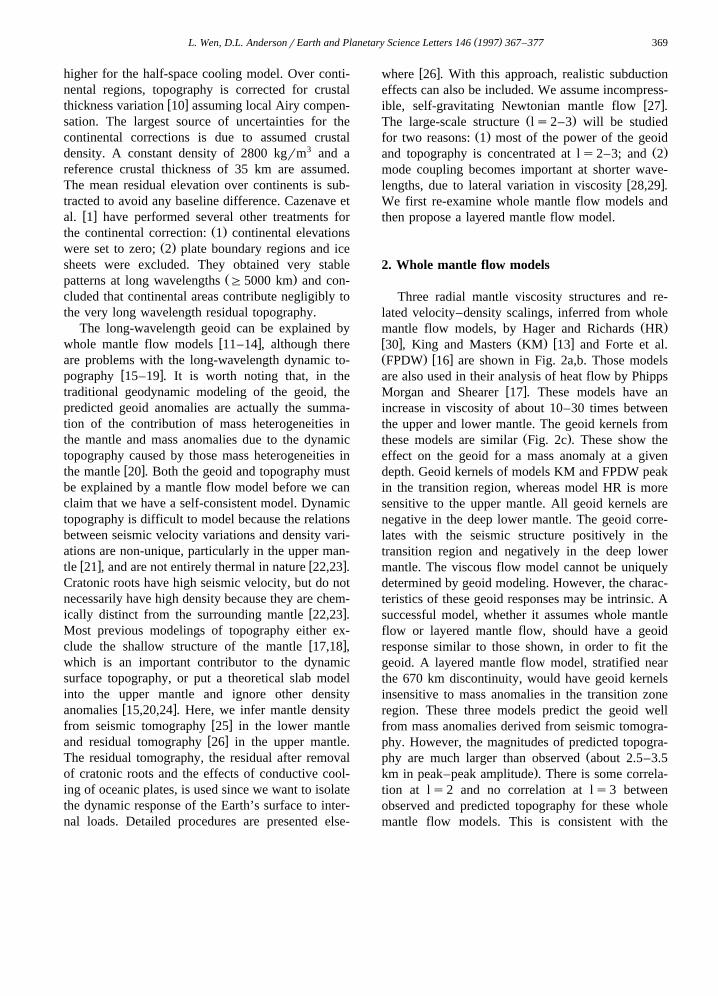
Three radial mantle viscosity structures and re-lated velocity–density scalings, inferred from whole

Ž .mantle flow models, by Hager and Richards HRw x Ž . w x30 , King and Masters KM 13 and Forte et al.Ž . w xFPDW 16 are shown in Fig. 2a,b. Those modelsare also used in their analysis of heat flow by Phipps

w xMorgan and Shearer 17 . These models have anincrease in viscosity of about 10–30 times betweenthe upper and lower mantle. The geoid kernels from

Ž .these models are similar Fig. 2c . These show theeffect on the geoid for a mass anomaly at a givendepth. Geoid kernels of models KM and FPDW peakin the transition region, whereas model HR is moresensitive to the upper mantle. All geoid kernels arenegative in the deep lower mantle. The geoid corre-lates with the seismic structure positively in thetransition region and negatively in the deep lowermantle. The viscous flow model cannot be uniquelydetermined by geoid modeling. However, the charac-teristics of these geoid responses may be intrinsic. Asuccessful model, whether it assumes whole mantleflow or layered mantle flow, should have a geoidresponse similar to those shown, in order to fit thegeoid. A layered mantle flow model, stratified nearthe 670 km discontinuity, would have geoid kernelsinsensitive to mass anomalies in the transition zoneregion. These three models predict the geoid wellfrom mass anomalies derived from seismic tomogra-phy. However, the magnitudes of predicted topogra-

Žphy are much larger than observed about 2.5–3.5.km in peak–peak amplitude . There is some correla-

tion at ls2 and no correlation at ls3 betweenobserved and predicted topography for these wholemantle flow models. This is consistent with the

( )L. Wen, D.L. AndersonrEarth and Planetary Science Letters 146 1997 367–377370

w xresults of other recent studies 17–19 . A large am-plitude dynamic topography is also predicted for the

w xdensity model inferred from past subduction 24 .It is obvious from effective topography kernels

Ž .Fig. 2d that current whole mantle convection mod-els cannot predict both the geoid and residual topog-raphy simultaneously. The contribution from lowermantle heterogeneity, by itself, already exceeds theobserved residual topography for these whole mantleconvection models. This is evident also in previous

Ž . Ž .Fig. 2. a Radial viscosity structure and b corresponding veloc-Ž .ity–density scaling E ln rrE lnV for three viscosity models,s

w xassuming whole mantle flow: HRsHager and Richards 30 ;w x w xKMsKing and Masters 13 ; and FPDW sForte et al. 16 ; and

Ž .the preferred viscosity models in this study WA1 and WA2 ,Ž .which assume layered mantle flow stratified at 920 km. c The

Ž .effective degree 2 geoid kernel and d the dynamic topographykernel for each model. These kernels are multiplied by the corre-sponding velocity–density scalings for that depth. Qualitatively,the area bounded by the effective topography kernel and verticalaxis can be viewed as the amplitude of predicted dynamic topog-raphy. Note that the layered mantle flow model, WA, predictsmuch less dynamic topography than whole mantle flow modelsdo.

Ž . w xFig. 3. a The spectra of nonhydrostatic geoid 6 and residualw xtopography 1 and predicted topography by layered mantle flow

Ž .model WA2 and whole mantle flow model HR. b The compari-son of the spectrum of seismologically inferred topographyŽ . w xTopo660a 31 and spectra of the topography at 670 km calcu-

w x w xlated using the viscosity structure of TMC 18 and HR 30 , if theundulation of the 670 km seismic discontinuity is responsible forthe excessive topography at the surface, produced by those mod-els. We assume that the excessive topography is equal to that

Žobserved i.e. whole mantle flow models produce twice as much.dynamic topography as observed . Note the different behavior.

This implies that ‘‘excess topography’’ at the surface, if there isany, cannot come from as deep as 670 km. For comparison,spectra are normalized to degree ls2. Note the logarithmic scale.

work. We have attempted to find a whole mantleflow model that satisfies both the geoid and thedynamic topography. We use the above models forviscosity and assume that the velocity–density scal-ings are constants in the depth intervals 0–400 km,400–670 km and 670 km–CMB. We attempted aleast-squares fit to the geoid by searching over arange of velocity–density scaling constants. We wereunable to reduce the amplitude of the predictedtopography. We were unable to obtain a satisfactoryfit to both the geoid and the topography at ls2–3with whole mantle convection by performing aleast-squares fit to both the geoid and topography.There is no correlation between residual topographyand predicted dynamic topography at ls3 in anycase.

3. The origin of dynamic topography

The spectra of residual topography and geoid areshown in Fig. 3a. The amplitude of the geoid de-

( )L. Wen, D.L. AndersonrEarth and Planetary Science Letters 146 1997 367–377 371

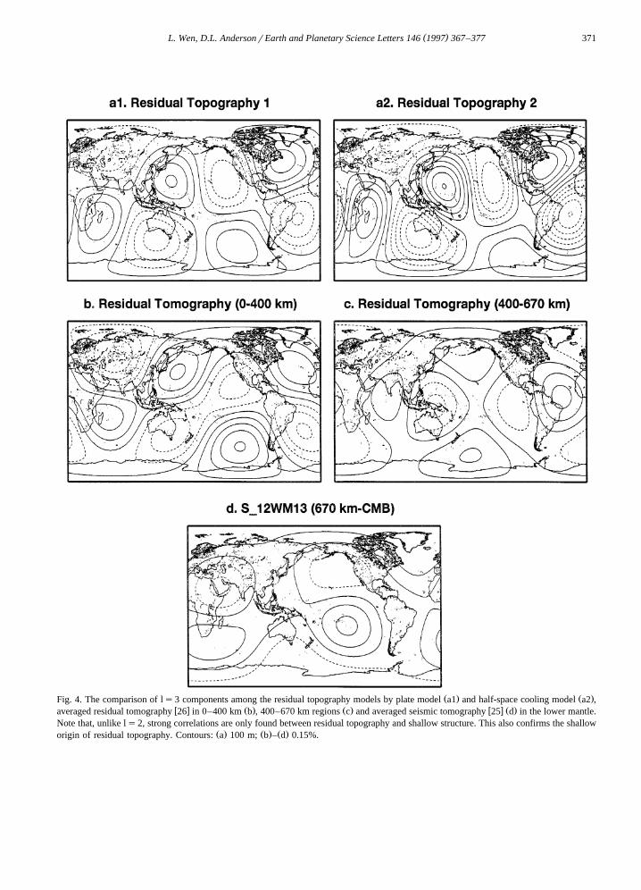
Ž . Ž .Fig. 4. The comparison of ls3 components among the residual topography models by plate model a1 and half-space cooling model a2 ,w x Ž . Ž . w x Ž .averaged residual tomography 26 in 0–400 km b , 400–670 km regions c and averaged seismic tomography 25 d in the lower mantle.

Note that, unlike ls2, strong correlations are only found between residual topography and shallow structure. This also confirms the shallowŽ . Ž . Ž .origin of residual topography. Contours: a 100 m; b – d 0.15%.

( )L. Wen, D.L. AndersonrEarth and Planetary Science Letters 146 1997 367–377372

creases much faster toward short wavelengths thanthat of residual topography. The long-wavelengthsignal senses deeper than short wavelengths. Forpotential fields, the faster the spectrum decreaseswith inverse wavelength, the deeper the origin ofanomalies. For example, the magnetic field comesfrom the core and the spectrum decreases muchfaster than the geoid and topography spectra. Thedifferent behaviors of the spectra of geoid and resid-ual topography imply that dynamic topography iscontrolled by density variations in the shallow man-

w xtle. Thoroval et al. 18 recently proposed that theundulation of the 670 km discontinuity is responsiblefor the excessive topography at the surface producedby whole mantle flow models. Spectral analysis isuseful in discussing this possibility since it dependsonly on the viscosity model. Let us assume thatwhole mantle flow models predict twice as muchdynamic topography as observed. In this case, halfconfirms the observation and we will attribute theother half to the topographic effect of the 670 kmdiscontinuity. In order to produce the excess topogra-phy that we have assumed, we can quantitativelycalculate the spectral behavior of the undulation ofthe 670 km discontinuity for the various viscositystructure models. Fig. 3b shows examples of thespectral behavior of the 670 km discontinuity for

w xviscosity models of Thoroval et al. 18 and Hagerw xand Richards 30 . This indicates that, if the undula-

tion of the 670 km discontinuity is responsible forthe ‘‘excess topography’’ predicted by whole mantleflow models, then the signal increases at short wave-lengths for the topography at 670 km. Geoid, topog-raphy, subduction history and seismic tomographyshow that large-scale features dominate mantle con-vection. It is hard to believe that small scale domi-nates for topography at the 670 km discontinuity.The spectrum of the seismologically inferred topog-

w xraphy of the 670 km discontinuity 31 is also shownfor comparison. This quantitative analysis indicatesthat, if a certain boundary is responsible for the‘‘excess topography’’ at the surface produced bywhole mantle flow models, this boundary cannot beas deep as 670 km. The incorporation of the topogra-phy of the 410 km and 670 km discontinuities intothe geodynamical modeling also produces large am-

w xplitude surface dynamic topography 17 . It is worthnoting that heterogeneities in the upper 300 km were

w xnot included in those models 17,18 . These hetero-geneities, however, have a significant influence ondynamic topography.

It is also worth noting that explaining the patternof the dynamic topography is as important as match-ing the amplitude of dynamic topography for a con-vection model. At ls2, the residual topography

w xcorrelates with lower mantle seismic tomography 1 .However, the correlations are even better at shallowdepths. No correlations are found in the transitionzone region. The connection between deep mantlestructure and shallow mantle structure at this degreeŽ . w xls2 is unclear 26 and this confuses the situation.However, the pattern at ls2,3 allows us to discrimi-nate between the various proposals for the origin ofdynamic topography. Fig. 4 shows the sphericalharmonic degree ls3 component of the residualtopography corrected by different subsidence laws inthe oceans, averaged residual seismic tomography inthe top 400 km, transition zone region, and seismictomography in the lower mantle. There are verygood correlations between residual topography andshallow seismic residual tomography, with topo-graphic lows corresponding with high velocities andtopographic highs corresponding with low velocities.The shallow origin of residual topography can beseen clearly from the direct comparison of patternsof residual topography and seismic tomography. Ifone excludes the structure in the upper 300 km, it ishard to imagine that one can find a viscous flowmodel that predicts the correct pattern of dynamictopography from a density model inferred from seis-mic tomography for the rest of the mantle.

4. Layered mantle flow model

Shallow origin and small amplitude of dynamicŽ .topography have two possible explanations: 1

Whole mantle flow with a very high viscosity lowermantle. Such a model would be rejected by the

Ž .geoid. 2 Layered mantle flow with the upper andlower part of the mantle mechanically decoupled.With a large viscosity jump from the upper to lowermantle, the Earth’s surface does not respond to themass heterogeneities in the lower mantle for layered

w xmantle flow model. Fleitout 32 pointed out that themagnitudes of observed surface topography and in-

( )L. Wen, D.L. AndersonrEarth and Planetary Science Letters 146 1997 367–377 373

tra-plate stress are more compatible with a two-layerconvective mantle, with the lower mantle mechani-cally decoupled from the lithosphere and unable toinduce tectonic stress.

Previous discussions about possible geodynamicbarriers have focused on the 670 km discontinuity.Layered mantle convection models, stratified at 670km, produce excessive topography at this boundaryw x w x30 or poor fits to the geoid 12 . The incorporationof the seismologically inferred topography on the

w x670 km discontinuity 33 seems to rule out thisboundary as the dividing line between shallow anddeep mantle convection. Many regional high resolu-tion seismic tomography studies also reveal highvelocity anomalies below this discontinuity beneath

w xseveral subduction zones 34,35 . The 670 km dis-continuity is primarily due to an endothermic phasechange between the spinel and post-spinel forms of

w xolivine 36 . There is no requirement that composi-tional difference must set in at this depth. For exam-ple, a chemical barrier may exist deeper and beunrelated to the present position of the spinel–post-spinel phase boundary.

There are now several independent lines of evi-dence for an important geodynamic boundary in themid-mantle: seismic evidence for the presence and

w xhigh relief of a 920 km discontinuity 37,38 ; correla-tions between subduction history in the past 130 Maand seismic tomography at about 800–1100 km

w xdepths in the mantle 39 ; decorrelation of seismicw xtomographic models at 900–1000 km depth 40 and

reversal of thermal fluctuations at a depth of aboutw x850 km 41 . It is of interest to see if a barrier near

these depths can satisfy the geoid and topographicdata.

We applied rheological models, similar to that ofw x Ž .Hager and Richards 30 WA1 and WA2, Fig. 2a .

Ž .The velocity–density scaling factors E ln rrE lnVs

are assumed to be constants for the depth intervals,0–400 km, 400–670 km and 670 km–CMB. Thesethree constants were obtained by a least-squares fitto both the geoid and residual topography, assuminga layered mantle convection with a boundary at the920 seismic discontinuity. WA1 and WA2 wereapplied for residual topography models corrected bythe plate model and half-space model separately.

Our best fit velocity–density scaling factors aresimilar to these for the whole mantle flow model of

w x Ž .Forte et al. 12 Fig. 2b . The effective geoid kernelis very similar to those of whole mantle convection

w x Ž .models 12,13,30 Fig. 2c . This indicates the lackof uniqueness of geoid modeling in discriminatingbetween whole mantle and layered mantle flow.Remarkable differences between layered mantle andwhole mantle flow models are evident in the topog-

Ž .raphy kernels Fig. 2d . For the whole mantle con-vection models, the topography kernels are sensitiveto the whole mantle. For layered mantle convectionmodels, with a viscosity jump of about a factor of

Ž .10–30 in the lower mantle WA1 and WA2 , andchemical stratification at 920 km, the topographykernel is only sensitive to the upper mantle; that is,only density anomalies in the upper mantle con-tribute to most of the dynamic topography. Thelower mantle contributes little to the surface dynamictopography for layered mantle flow model WA2.The predicted dynamic topography for layered man-tle flow models, at ls2–3, are shown in Fig. 1b,d.The predicted and observed dynamic topography havehighs in the central Pacific and in southeast Africaand large depressions in Eurasia, south Australia andSouth America. At ls2,3, the correlation coeffi-cients between predicted and observed exceed the95% confidence level for the topography correctedby the plate model, and exceed the 90% confidencelevel for topography corrected by the half-spacecooling model. The predicted geoid is very similar

Ž .for both models WA1 and WA2 . Therefore, onlythe prediction from model WA1 is presented in Fig.1f. The correlation coefficients between observedand predicted geoid exceed the 95% confidence levelat ls3 and the 93% confidence level at ls2. Thepredictions of geoid and topography reproduce notonly the patterns, but also the amplitudes as well.The spectrum of predicted dynamic topography formodel WA2 is shown in Fig. 3a. An example for thespectral behavior of dynamic topography predicted

Ž .by the whole mantle flow model HR is also shownfor comparison. The layered mantle convection flowmodel is more consistent with the spectral behaviorof the observed topography.

The topographic relief at the 670 km endothermicphase change is a second-order effect in geoid andtopography modeling. But it is important in predict-ing the dynamic topography at a deeper chemicaldiscontinuity. We incorporate the topography at 670

( )L. Wen, D.L. AndersonrEarth and Planetary Science Letters 146 1997 367–377374

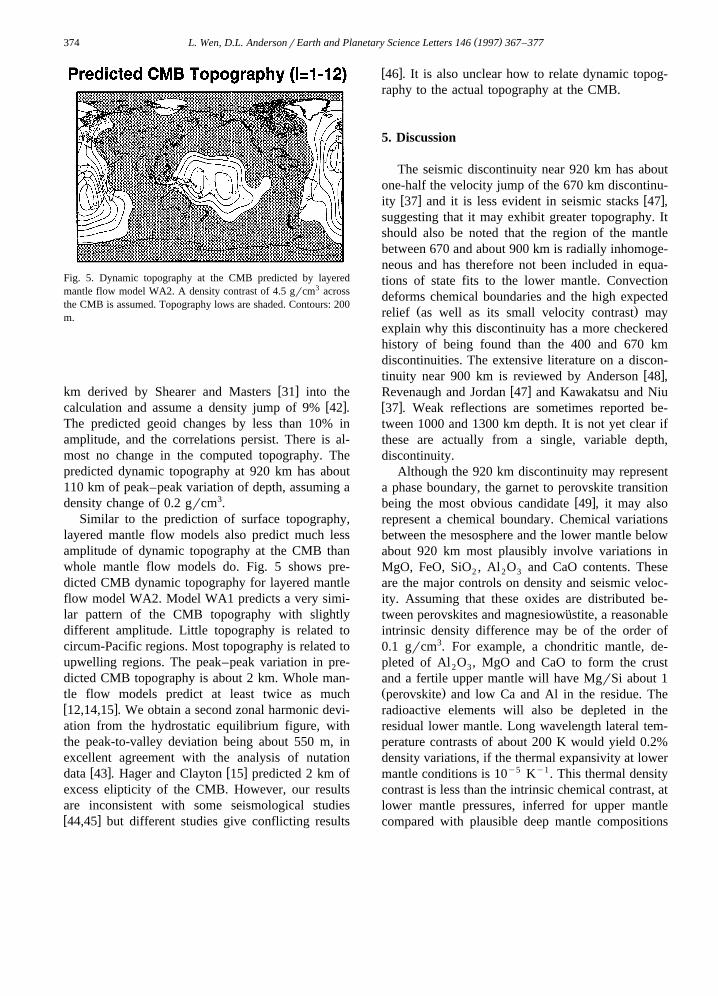
Fig. 5. Dynamic topography at the CMB predicted by layeredmantle flow model WA2. A density contrast of 4.5 grcm3 acrossthe CMB is assumed. Topography lows are shaded. Contours: 200m.

w xkm derived by Shearer and Masters 31 into thew xcalculation and assume a density jump of 9% 42 .

The predicted geoid changes by less than 10% inamplitude, and the correlations persist. There is al-most no change in the computed topography. Thepredicted dynamic topography at 920 km has about110 km of peak–peak variation of depth, assuming adensity change of 0.2 grcm3.

Similar to the prediction of surface topography,layered mantle flow models also predict much lessamplitude of dynamic topography at the CMB thanwhole mantle flow models do. Fig. 5 shows pre-dicted CMB dynamic topography for layered mantleflow model WA2. Model WA1 predicts a very simi-lar pattern of the CMB topography with slightlydifferent amplitude. Little topography is related tocircum-Pacific regions. Most topography is related toupwelling regions. The peak–peak variation in pre-dicted CMB topography is about 2 km. Whole man-tle flow models predict at least twice as muchw x12,14,15 . We obtain a second zonal harmonic devi-ation from the hydrostatic equilibrium figure, withthe peak-to-valley deviation being about 550 m, inexcellent agreement with the analysis of nutation

w x w xdata 43 . Hager and Clayton 15 predicted 2 km ofexcess elipticity of the CMB. However, our resultsare inconsistent with some seismological studiesw x44,45 but different studies give conflicting results

w x46 . It is also unclear how to relate dynamic topog-raphy to the actual topography at the CMB.

5. Discussion

The seismic discontinuity near 920 km has aboutone-half the velocity jump of the 670 km discontinu-

w x w xity 37 and it is less evident in seismic stacks 47 ,suggesting that it may exhibit greater topography. Itshould also be noted that the region of the mantlebetween 670 and about 900 km is radially inhomoge-neous and has therefore not been included in equa-tions of state fits to the lower mantle. Convectiondeforms chemical boundaries and the high expected

Ž .relief as well as its small velocity contrast mayexplain why this discontinuity has a more checkeredhistory of being found than the 400 and 670 kmdiscontinuities. The extensive literature on a discon-

w xtinuity near 900 km is reviewed by Anderson 48 ,w xRevenaugh and Jordan 47 and Kawakatsu and Niu

w x37 . Weak reflections are sometimes reported be-tween 1000 and 1300 km depth. It is not yet clear ifthese are actually from a single, variable depth,discontinuity.

Although the 920 km discontinuity may representa phase boundary, the garnet to perovskite transition

w xbeing the most obvious candidate 49 , it may alsorepresent a chemical boundary. Chemical variationsbetween the mesosphere and the lower mantle belowabout 920 km most plausibly involve variations inMgO, FeO, SiO , Al O and CaO contents. These2 2 3

are the major controls on density and seismic veloc-ity. Assuming that these oxides are distributed be-tween perovskites and magnesiowustite, a reasonable¨intrinsic density difference may be of the order of0.1 grcm3. For example, a chondritic mantle, de-pleted of Al O , MgO and CaO to form the crust2 3

and a fertile upper mantle will have MgrSi about 1Ž .perovskite and low Ca and Al in the residue. Theradioactive elements will also be depleted in theresidual lower mantle. Long wavelength lateral tem-perature contrasts of about 200 K would yield 0.2%density variations, if the thermal expansivity at lowermantle conditions is 10y5 Ky1. This thermal densitycontrast is less than the intrinsic chemical contrast, atlower mantle pressures, inferred for upper mantlecompared with plausible deep mantle compositions

( )L. Wen, D.L. AndersonrEarth and Planetary Science Letters 146 1997 367–377 375

w x50 . The density difference at lower mantle pres-sures, between various plausible chemical models ofthe upper and lower mantle, ranges from 2.6% to 5%w x50 . This is enough to stratify mantle flow.

An increase in SiO or a decrease in MgO content2

will tend to raise seismic velocities. The effect ofFeO depends on its spin state and metallic nature.Assuming that Al O stabilizes the garnet structure2 3

w xto about 1000 km depth 49,50 , and assuming fur-ther that magma extraction has depleted the lower

Ž .mantle presumably during accretional melting inAl O and CaO, and that the original mantle was2 3

more chondritic than the current upper mantle, then aSiO -rich and CaO, Al O -poor, and U, Th, K-poor,2 2 3

lower mantle is expected. The FeO budget of thelower mantle depends not only on its melt extractionhistory but also its subsequent interaction with thecore and core-forming material in its early history. Itis, in fact, difficult to imagine how a homogeneousmantle may have formed, particularly consideringthe efficient extraction of the crust-forming elementsupwards and the core-forming elements downwards.Thermal expansion is high at upper mantle pressures;this, plus the effects of partial melting, means thatcompositional layers can be breached and potentiallymixed with surrounding mantle. Pressure suppressesthermal expansivity and chemical discontinuities canbe expected to be more permanent in the deepmantle.

There are various arguments for and against strati-fied mantle convection. Small intrinsic density con-trasts between layers can easily be overcome atlower pressures. The effect of pressure on thermalexpansivity makes this more difficult at high pres-sures. Many of the arguments against stratified con-vection are actually arguments against the 670 kmlevel being the boundary. These arguments do notapply if the convection interface occurs nearer to 920km. The possibility of an important geodynamicboundary several hundred kilometers deeper than themajor seismic discontinuity at 670 km is consistentwith electrical conductivity and viscosity data, aswell as with 1D and 3D seismic modeling. Forexample, the viscosity may rise rapidly below 800–

w x900 km 51 . Layered mantle convection serves toinsulate the lower mantle and is less efficient at heat

w xremoval than whole mantle convection 52 . Conse-quently, two-layer convection implies a lower mantle

w xdepleted of radioactive heat sources 52 , consistentw xwith the differentiation during accretion model 53 .

6. Conclusion

The amplitude of dynamic topography predictedby previous viscosity models involving whole mantleflow is much larger than observed. We are unable tofind reasonable velocity–density scalings to fit thegeoid and residual topography for whole mantle flowmodels. This is consistent with recent studies on

w xtopography 17–19 . We show that the seismic to-mography at shallow depths, once corrected for thechemical effects of cratonic roots and thermal cool-ing of oceanic lithosphere, exhibit slow velocitiesthat are well correlated with uplifted regions at long

Ž .wavelengths ls2,3 . The spectrum of residual to-pography also reveals the shallow origin of dynamictopography. The long-wavelength dynamic topogra-phy is controlled by density variations in the uppermantle, whereas the long-wavelength geoid is con-trolled by density throughout the mantle. Layeredmantle convection stratified at about 920 km pro-vides a self-consistent geodynamic model in explain-ing the long-wavelength geoid and topography.

Acknowledgements

We thank Anny Cazenave for the residual topog-raphy data, Scott King for the viscosity structure andMichael Gurnis, David Stevenson and Craig Scrivnerfor reviews. This work was funded by NSF grantEAR 92-18390. Contribution No. 5598, Division ofGeological and Planetary Sciences, California Insti-

[ ]tute of Technology. RV

References

w x1 A. Cazenave, A. Souriau and K. Dominh, Global coupling ofEarth surface topography with hotspots, geoid and mantleheterogeneities, Nature 340, 54–57, 1989.

w x2 A. Cazenave and B. Lago, Long wavelength topography,seafloor subsidence and flattening, Geophys. Res. Lett. 18,1257–1260, 1991.

w x3 P. Colin and L. Fleitout, Topography of the ocean floor:thermal evolution of the lithosphere and interaction of mantle

( )L. Wen, D.L. AndersonrEarth and Planetary Science Letters 146 1997 367–377376

heterogeneities with the lithosphere, Geophys. Res. Lett. 11,1961–1964, 1990.

w x4 M. Kido and T. Seno, Dynamic topography compared withresidual depth anomalies in oceans and implications forage–depth curves, Geophys. Res. Lett. 21, 717–720, 1994.

w x5 M. Gurnis, Bounds on global dynamic topography fromPhanerozoic flooding of continental platforms, Nature 344,754–756, 1990.

w x6 J.G. Marsh, F.J. Lerch, B.H. Putney, T.L. Felsentreger andB.V. Sanchez, The GEM-T2 gravitational model, J. Geophys.Res. 95, 22,043–22,071, 1990.

w x7 C.A. Stein and S. Stein, A model for the global variation inoceanic depth and heat flow with lithospheric age, Nature359, 123–129, 1992.

w x8 J.C. Marty and A. Cazenave, Regional variations in subsi-dence rate of lithospheric plates: Implication for thermalcooling models, Earth Planet. Sci. Lett. 94, 301–315, 1989.

w x9 A. Cazenave, K. Dominh, C.J. Allegre and J.G. Marsh,`Global relationship between oceanic geoid and topography, J.Geophys. Res. 91, 11,439–11,450, 1986.

w x10 O. Cadek and Z. Martinee, Spherical harmonic expansion ofthe Earth’s crustal thickness up to degree and order 30, Stud.Geophys. Geod. 35, 151–165, 1991.

w x11 B.H. Hager, R.W. Clayton, M.A. Richards, R.P. Comer andA.M. Dziewonski, Lower mantle heterogeneity, dynamic to-pography and the geoid, Nature 313, 541–545, 1985.

w x12 A.M. Forte, A.M. Dziewonski and R.L. Woodward, A spher-ical structure of the mantle tectonics, nonhydrostatic geoidand the topography of the core-mantle boundary, in: Dynam-ics of the Earth’s Deep Interior and Earth Rotation, AGUGeophys. Monogr. Ser. 72, 135–166, 1993.

w x13 S.D. King and G. Masters, An inversion for radial viscositystructure using seismic tomography, Geophys. Res. Lett. 19,1551–1554, 1992.

w x14 Y. Ricard and B. Wuming, Inferring the viscosity and the3-D density structure of the mantle from the geoid, topogra-phy, and plate velocities, Geophys. J. Int. 105, 561–571,1991.

w x15 B.H. Hager and R.W. Clayton, Constraints on the structureof mantle convection using seismic observations, flow mod-els, and the geoid, in: Mantle Convection, W.R. Peltier, ed.,pp. 657–763, Gordon and Breach, New York, NY, 1989.

w x16 A.M. Forte, W.R. Peltier, A.M. Dziewonski and R.L. Wood-ward, Dynamic surface topography: A new interpretationbased upon mantle flow models derived from seismic tomog-raphy, Geophys. Res. Lett. 20, 225–228, 1993.

w x17 J. Phipps Morgan and P.M. Shearer, Seismic and geoidconstraints on mantle flow: Evidence for whole mantle con-vection, J. Geophys. Res., submitted, 1994.

w x18 C. Thoraval, P. Machetel and A. Cazenave, Locally layeredconvection inferred from dynamic models of the Earth’smantle, Nature 375, 777–779, 1995.

w x19 Y.L. Stunff and Y. Ricard, Topography and geoid due tolithosphere mass anomalies, Geophys. J. Int. 122, 982–990,1995.

w x20 B.H. Hager, Subducted slabs and the geoid: constraints on

mantle rheology and flow, J. Geophys. Res. 89, 6003–6015,1984.

w x21 A.M. Forte, A.M. Dziewonski and R.J. O’Connell, Conti-nent–ocean chemical heterogeneity in the mantle based onseismic tomography, Science 268, 386–388, 1995.

w x22 T.H. Jordan, The continental tectosphere, Rev. Geophys.Space Phys. 13, 1–12, 1975.

w x23 D.L. Anderson and J.D. Bass, Mineralogy and compositionin the upper mantle, Geophys. Res. Lett. 11, 637–640, 1984.

w x24 Y. Ricard, M.A. Richards, C. Lithgow-Bertelloni and Y.LeStunff, A geodynamic model of mantle density hetero-geneity, J. Geophys. Res. 98, 21,895–21,909, 1993.

w x25 W.J. Su, R.L. Woodward and A.M. Dziewonski, Degree 12model of shear velocity heterogeneity in the mantle, J.Geophys. Res. 99, 6945–6980, 1994.

w x26 L. Wen and D.L. Anderson, Slabs, hotspots, cratons andmantle convection revealed from residual seismic tomogra-phy in the upper mantle, Phys. Earth Planet. Inter. 99,131–143, 1997.

w x27 M.A. Richards and B.H. Hager, Geoid anomalies in a dy-namic Earth, J. Geophys. Res. 89, 5987–6002, 1984.

w x28 M.A. Richards and B.H. Hager, Effects of lateral viscosityvariations on long-wavelength geoid anomalies and topogra-phy, J. Geophys. Res. 94, 10,299–10,313, 1989.

w x29 S. Zhang and U.R. Christensen, The effect of lateral viscosityvariations on geoid topography and plate motions induced bydensity anomalies in the mantle, Geophys. J. Int. 114, 531–547, 1993.

w x30 B.H. Hager and M.A. Richards, Long-wavelength variationsin Earth’s geoid: physical models and dynamical implica-tions, Philos. Trans. R. Soc. London A 328, 309–327, 1989.

w x31 P.M. Shearer and G. Masters, Global mapping of topographyon the 660 km discontinuity, Nature 355, 791–796, 1992.

w x32 L. Fleitout, Source of lithospheric tectonic stress, Philos.Trans. R. Soc. London A 337, 73–81, 1991.

w x33 J. Phipps Morgan and P.M. Shearer, Seismic constraints onmantle flow and topography of the 660 km discontinuity:Evidence for whole mantle convection, Nature 365, 506–511,1993.

w x34 T.H. Jordan and W.S. Lynn, A velocity anomaly in the lowermantle, J. Geophys. Res. 79, 2,679–2,685, 1974.

w x35 R. van der Hilst, Complex morphology of subducted litho-sphere in the mantle beneath the Tonga trench, Nature 374,154–157, 1995.

w x36 D.L. Anderson, Phase change in the upper mantle, Science157, 1165–1173, 1967.

w x37 H. Kawakatsu and F. Niu, Seismic evidence for a 920-kmdiscontinuity in the mantle, Nature 371, 301–305, 1994.

w x38 H. Kawakatsu and F. Niu, Depth variation of ‘‘the 920 kmdiscontinuity’’ in the mid-mantle, EOS Trans. AGU 76,F382, 1995.

w x39 L. Wen and D.L. Anderson, The fate of the slabs inferredfrom 130 Ma subduction and seismic tomography, EarthPlanet. Sci. Lett. 133, 185–198, 1995.

w x40 M.H. Ritzwoller and E.M. Lavely, Three-dimension seismicmodels of the Earth’s mantle, Rev. Geophys. 33, 1–66, 1995.

( )L. Wen, D.L. AndersonrEarth and Planetary Science Letters 146 1997 367–377 377

w x41 S. Balachandar, Eigenfunctions of the two-point correlationsfor optimal characterization of mantle convection: possibilityof additional discontinuity around 850 km, EOS Trans. AGU76, F618, 1995.

w x42 A.M. Dziewonski and D.L. Anderson, Preliminary referenceEarth model, Phys. Earth Planet. Inter. 25, 297–356, 1981.

w x43 C. R. Gwinn, T.A. Herring and I.I. Shapiro, Geodesy byradio interferometry: Studies of the forced nutations of theEarth 2. Interpretation, J. Geophys. Res. 91, 4755–4765,1986.

w x44 A. Morelli and A.M. Dziewonski, Topography of the core–mantle boundary and lateral heterogeneity of the liquid core,Nature 325, 678–683, 1987.

w x45 D.J. Doornbos and T. Hilton, Models of the core–mantleboundary and the travel times of internally reflected corephases, J. Geophys. Res. 94, 15,741–15,751, 1989.

w x46 J.E. Vidale and H.M. Benz, A sharp and flat section of thecore–mantle boundary, Nature 359, 627–629, 1992.

w x47 J. Revenaugh and T.H. Jordan, Mantle layering from ScS

reverberations: 2 The transition zone, J. Geophys. Res. 96,19,763–19,780, 1991.

w x48 D.L. Anderson, Recent evidence concerning the structure andcomposition of the Earth’s mantle, in: Physics and Chemistryof the Earth, 6, pp. 1–131, Pergamon, Oxford, 1966.

w x49 S.E. Kesson, J.D. Fitz Gerald and J.M. Shelley, Mineralchemistry and density of subducted basaltic crust at lower-mantle pressures, Nature 372, 767–769, 1995.

w x50 R. Jeanloz, Effects of phase transitions and possible composi-tional changes on the seismological structure near 650 kmdepth, Geophys. Res. Lett. 18, 1743–1746, 1991.

w x51 E.R. Ivins, C.G. Sammis and C.F. Yoder, Deep mantleviscous structure with prior estimate and satellite constraint,J. Geophys. Res. 98, 4579–4609, 1993.

w x52 T. Spohn and G. Schubert, Modes of mantle convection andthe removal of heat from the Earth’s interior, J. Geophys.Res. 87, 4682–4696, 1982.

w x53 D.L. Anderson, Theory of the Earth, 366 pp., Blackwell,Boston, MA, 1989.