Earth Planets Space, 50, 1055–1065, 1998

Synthetic tests of geoid-viscosity inversion: A layered viscosity case

Motoyuki Kido1 and Satoru Honda2

1Ocean Research Institute, University of Tokyo, 164-8639, Japan2Department of Earth and Planetary System Science, University of Hiroshima, 739-8526, Japan

(Received April 2, 1998; Revised November 2, 1998; Accepted November 5, 1998)

We revisited the resolving power of viscosity inversion in terms of geoid misfit in a 2-D Cartesian geometry underthe assumption that the mantle viscosity is laterally stratified. Firstly, we considered a simple case of two viscositylayers only, which is described by two parameters of the amount and the depth of the viscosity jump. The uniquenessof the inversion was examined by evaluating misfits between the reference geoid for a reference viscosity and thatfor a viscosity described by the changing two parameters. The misfits are mapped into 2-D model space as a functionof the two parameters. Three types of density distribution are tested; they are vertically constant (1), taken from atomographic model (2), and the same but includes artificial noise (3). We found that, at least for this simple case, theviscosity solution keeps unique in the entire 2-D model space using whole degree band (1–8) of geoid. This holdseven if the artificial noise is rather large (70%), though the solution is slightly different from the reference viscosity.However, we also observed non-uniqueness, such as trade-off between the two parameters, when individual degreecomponents of geoid are concerned. In the next, we employed a more realistic viscosity structure, having seveniso-viscous layers. It is no longer possible to describe 6-D model space easily. Therefore we tried to reconstruct areference viscosity from the reference geoid using genetic algorithm search. According to this analysis, nearly thesame solution with the reference viscosity can be reconstructed, while solutions apart from the reference viscositywith increase of noise in the density distribution.

1. IntroductionOver the last decade, a great number of studies has been

made to investigate the mantle viscosity profile inferred fromobserved geoid and seismic tomographic data (e.g., Richardsand Hager, 1984). Currently there is a great progress in devel-oping new methods to analyze the mantle viscosity with morerealistic conditions, taking compressibility (Forte and Peltier,1991; Thoraval et al., 1994; Corrieu et al., 1995; Panasyuket al., 1996), lateral viscosity variation (Ricard et al., 1988;Richards and Hager, 1989; Ricard et al., 1991; Ribe, 1992;Zhang and Christensen, 1993; Forte and Peltier, 1994), non-linear rheology (Cadek et al., 1993), and the 660 km discon-tinuity (Thoraval et al., 1995; Cadek et al., 1997; Forte andWoodward, 1997; Wen and Anderson, 1997) into account.The accuracy of tomographic models has also been improvedsignificantly. However, most of the studies present quite dif-ferent viscosity profiles, and there is no agreement exceptthat the lower mantle would be higher viscous than the uppermantle.

This discrepancy mainly comes from the used densitymodel. Usually density models are simply converted fromvelocity anomalies derived from tomographic models usinga linear velocity-density relation, which can be a functionof depth. On the contrary, some gropes employ a prioridensity anomalies for a certain part of the mantle. For twotypical studies, see King and Masters (1992) and Hager andRichards (1989) for example. While the former converted

Copy right c© The Society of Geomagnetism and Earth, Planetary and Space Sciences(SGEPSS); The Seismological Society of Japan; The Volcanological Society of Japan;The Geodetic Society of Japan; The Japanese Society for Planetary Sciences.

velocity anomalies into a density model for the entire man-tle, the latter imposed high density anomalies in the uppermantle associated with subducting slabs where low veloc-ity anomalies are observed in long wavelength tomographicmodels. These two density models are much different in theshallow upper mantle, and these force the obtained viscos-ity profiles are much different as well. King and Masters(1992) prefer low viscous transition zone, while Hager andRichards (1989) suggest a low viscous asthenosphere. Fur-ther work has been made to construct more realistic densitymodels, correcting for continental roots (Forte et al., 1995;Doin et al., 1996), using various geological data (Ricard etal., 1995), simulating past subduction history (Ricard et al.,1993). In spite of these studies and improvements of seismictomography results, large uncertainties in estimating densitystructure still remain due to the difficulty of interpreting theseismic velocity anomaly beneath cratons (Jordan, 1978) andsubduction zones (Karato, 1995).

Another reason for the existence of many different viscos-ity profiles is the progress in the inversion methods. Tradi-tional inversion techniques, such as calculating partial deriva-tives (e.g., Tarantola and Valette, 1982), tend to find solutionsstrongly depending on a starting model. Recent studies us-ing this type of inversion have been improved by introducinga penalty for the smoothness of the solution instead for thedistance from the starting model (King and Masters, 1992;Forte et al., 1994; Mitrovica and Forte, 1997). On the con-trary, Monte Carlo inversions (Ricard et al., 1989) can searchthe entire model space at the expense of much computationtime. Therefore only several free parameters can be allowedin it. Recently, a much more efficient inversion method,

1055

1056 M. KIDO AND S. HONDA: SYNTHETIC TESTS OF GEOID-VISCOSITY INVERSION

called genetic algorithm (GA), has been introduced to theEarth science community (e.g., Sen and Stoffa, 1992). GAhas the merit of Monte Carlo search, but drastically savescomputation time using dynamical weighting or probabilityof searching area in the model space. Details of the generalGA method can be found in Goldberg (1989). The GA hasfirst been applied to the geoid-viscosity inversion problem byKing (1995). He demonstrated the applicability of GA, butalso found multiple viscosity solutions even using the samedensity model. Kido and Cadek (1997) also applied GA tothis problem but for regional intermediate wavelength geoidanalysis, and found multiple solutions for regions where theresolution of the tomographic model is poor. In both studiesmultiple solutions are quite different to one another, whichindicates the non-uniqueness in this kind of inversion.

In this study, we examine the potential resolving power oruniqueness of the geoid-viscosity inversion in a 2-dimension-al Cartesian geometry. Moreover we also estimate the effectof noise in the density distribution on the resolving power. Atfirst, in Section 2, we show the nature of the uniqueness of thegeoid-viscosity inversion using a viscosity variation simplydepending on two parameters. Uniqueness of the problem isdiscussed based on maps representing the 2-D model spaceof misfit between the geoid for a reference viscosity and thatfor varying viscosities. In Section 3, we employed a more re-alistic case that viscosity can depend on six parameters. Herewe conduct synthetic inversions using GA to reconstruct thereference viscosity instead of mapping the entire model spacelike in the case of two parameters. In both cases, we also testhow noise in the density distribution devaluate the resolvingpower of the inversion, which corresponds to uncertaintiesin the interpretation of seismic velocity anomalies.

2. A Case for Two ParametersIn this section the complete morphology of 2-D model

space will be shown for two layers of viscosity variation. Atfirst, we describe the method of calculating the geoid anddensity distributions used in this study.

Geoid anomaly represents perturbation of the gravity po-tential field, which consists of the integral of density anoma-lies in the mantle (internal loads) and the deflection of all pos-sible density boundaries, e.g. Earth’s surface and the core-mantle boundary (CMB). These boundary deflections areinduced by the mantle flow, which is driven by the inter-nal loads. The instantaneous mantle flow can be calculatedwhen viscosity structure in the mantle is given. The basicequations are the equation of motion, continuity equation,constitutive law, and Poisson’s equation. Assuming a sim-ple model, such as no lateral viscosity variation and New-tonian mantle rheology, these equations can be separatelysolved for each wavelength component analytically. Thenthe resultant geoid can easily be calculated using the prop-agator matrix method. This method is described in Hagerand Clayton (1989) in detail. In this study, we assume anon self-gravitating incompressible fluid lies in a 2-D Carte-sian geometry whose aspect ratio is 8. Boundary conditionsare free slip and no vertical motion at the top and bottom,and periodical at the both sides. These assumptions lead toa rather simple approximation of the Earth’s mantle, there-fore the predicted geoid may significantly differ from the

observational geoid. However this fact does not prohibit toexamine the potential resolving power of the geoid-viscosityinversion, which is the goal of this paper. This is becausereference geoid is also calculated under the same conditionsas geoid to be compared.

We use four density distributions in this study. The firstone, here called CON, has no vertical density variation andhas only lateral variation assigned that all coefficients in itsFourier expansion will be 1. This density distribution is farfrom the Earth, however, is suitable to reveal nature of thepotential resolving power of the inversion. The second den-sity distribution, we call it TOM, is taken from an equatorialcross section of a recent tomographic model result for S-wave velocity (Li and Romanowicz, 1996). We horizontallyscaled the original cross section whose aspect ratio is 13.8to aspect ratio 8 in order to have the same conditions withthe density distribution CON. S-wave velocity anomaliesare converted to density anomalies assuming δρ/δv = 0.2(kg·m−3)/(m·s−1), where δρ is density anomaly and δv veloc-ity anomaly. This tomography derived density distribution isillustrated in Fig. 1. Stream lines, expected geoid, and bound-ary deformations for a reference viscosity are also drawn inthe figure. It simply has one viscosity jump of two order ofmagnitude at the depth of 660 km. We also prepare the otherdensity distribution ρnoise, which is derived by adding artifi-cial noise to TOM. TOM is taken from the equatorial crosssection and can be denoted as ρe(x, z), where x and z are hor-izontal and vertical coordinates respectively. Here, the noiseis also taken from the tomographic model but from a crosssection at the meridian and denoted as ρm(x, z). Then thedensity model including noise used in this study ρnoise(x, z)is defined as

ρnoise(x, z) = (1 − r) · ρe(x, z) + r · ρm(x, Z − z), (1)

where r is a constant and Z the height of the mantle to be con-sidered. As is defined in Eq. (1), the noise density ρm(x, z)has been turned upside down before the addition in order tobe as random as possible relative to ρe(x, z). We employedtwo noise levels of density distributions T30 and T70. The ris set to 0.3/(1+0.3) = 0.231 and 0.7/(1+0.7) = 0.412 sothat ratio of amplitude of the noise to the original density willbe 30% and 70%, respectively. All the density distributionused here are truncated up to degree 8 in the Fourier series.

As shown by the right hand small drawing in Fig. 1, thereference viscosity increases by a factor of 100 at the depth660 km. The reference geoids corresponding to the referenceviscosity calculated under the conditions described above aredrawn in the top part of Fig. 1.

Then we calculated geoids, which will be compared tothe reference geoid. As mentioned above, the used vis-cosity profile is a step function, which has two parame-ters; the depth of jump zjump and ratio of upper to lowerpart of mantle viscosity ηupp/ηlow. Using these descrip-tion, the reference viscosity can be represented that zjump =660 km and log10 (ηupp/ηlow) = −2. We calculated geoidsfor viscosity model space that zjump from 0 to 2900 km andlog10 (ηupp/ηlow) from −4 to 0.

Thus calculated geoid cal N is compared with the referencegeoid ref N for the reference viscosity. Root mean squares(RMS) of their difference normalized by RMS amplitude of

M. KIDO AND S. HONDA: SYNTHETIC TESTS OF GEOID-VISCOSITY INVERSION 1057

1058 M. KIDO AND S. HONDA: SYNTHETIC TESTS OF GEOID-VISCOSITY INVERSION

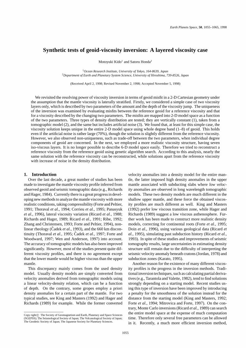
Fig. 2. Morphology of the root mean square (RMS) of the geoid misfit in 2-D model space for density distribution of (a) CON, (b) TOM, (c) T30,and (d) T70. See in the text for the notations of CON, TOM, T30, and T70. Two parameters in the model space are the depth of the viscosity jumpzjump for the vertical axis and the amount of the viscosity jump log10 (ηupp/ηlow) for the horizontal axis. The reference viscosity, zjump = 660 km andlog10(ηupp/ηlow) = −2, is indicated by a “+”. Value of the misfit is normalized by the RMS amplitude of the corresponding degree components of thereference geoid. For all the density distributions, individual degree components are shown as well as total degree components of 1–8, information ofwhich is depicted at the top of each panel. Supplemental broken contours are added to clearify the position of the global minimum in the top left panelfor (c) and (d).

the reference geoid, called misfit, are evaluated for the entiremodel space. The misfit D for components ranging fromdegree �1 to �2 is defined by

D�1,�2 =√√√√

∑�2�=�1

[ (reref N� − re

cal N�)2 + (imref N� − im

cal N�)2 ]∑�2�=�1

(reref N

2� + im

ref N2� )

,

(2)

M. KIDO AND S. HONDA: SYNTHETIC TESTS OF GEOID-VISCOSITY INVERSION 1059

Fig. 2. (continued).

where “re” and “im” mean the real and imaginary parts ofthe geoid coefficients in the Fourier series.

We plotted a contour map of the misfit D1,8 for the densitydistribution CON in the left top panel in Fig. 2(a). Verticaland horizontal axes represent the two parameters, zjump andlog10 (ηupp/ηlow) respectively, of the viscosity for calculatinggeoid. The position of the reference viscosity in the modelspace is indicated by a “+”. The small misfit region whereD1,8 < 0.1 is shown in white surrounded by dark regions.Scale of the shadings is indicated by a shading bar at the topof the figure. We also plotted misfit for the individual degree

component D� (= D�,� in Eq. (2)) in Fig. 2(a). Figures 2(b),2(c) and 2(d) are the same as Fig. 2(a) but for the densitydistributions of TOM, T30, and T70, respectively.

Looking at the D1,8 for CON in Fig. 2(a), the white areawhere D1,8 < 0.1 is small and centered at the position of thereference viscosity. This indicates that the inversion will givean unique and correct viscosity solution. For the individualdegree component of the misfit D� (� = 1 to 8), on the otherhand, we found that the white area tends to be stretchedout and the shape of it systematically shifts upward withincrease of degree while keeping the position of the reference

1060 M. KIDO AND S. HONDA: SYNTHETIC TESTS OF GEOID-VISCOSITY INVERSION

Fig. 2. (continued).

viscosity. This shows that a single wavelength componentof geoid is not able to resolve the viscosity profile if densitydistribution has no vertical variation.

For the misfit D1,8 for TOM in Fig. 2(b), the white areais also small as for the case CON. However, the behaviorof the misfit for the individual degree components are quitedifferent from that for CON. The systematic change of itsmorphology with degree is destroyed. The individual lowerdegree components, D1 and D2, already have strong con-strains to the viscosity solution at least for this simple caseof the two viscosity parameters. We observed a common

feature with the case CON that higher degree componentsof the geoid are poor to resolve the log10 (ηupp/ηlow). Thisis because the viscosity kernels for higher degrees are ratherinsensitive to such a large viscosity jump.

Finally in Figs. 2(c) and 2(d), we show the misfits for T30and T70, containing 30% and 70% of noise defined by Eq. (1)in the density distribution. It should be noted that the misfithere is the difference between the reference geoid for TOMand calculated geoid for T30 or T70. Therefore the misfitdoes not necessarily to have zero area even at the positionof the reference viscosity. However, some of the individual

M. KIDO AND S. HONDA: SYNTHETIC TESTS OF GEOID-VISCOSITY INVERSION 1061

Fig. 2. (continued).

degree components of misfit has the white region even forlarge noise level T70 in Fig. 2(d). We should mention thatall of these white regions do not coincide with the position ofthe reference viscosity. Especially for D1 of T30 in Fig. 2(c)and D3 of T70 in Fig. 2(d), white regions appear completelydifferent position from the reference viscosity. Neverthelesssuch strange behavior of the misfit in the model space forthe individual degree components, the global minimum ofthe misfit (indicated by supplemental contours) for the entiredegree band D1,8 is close to the position of the referenceviscosity both for T30 and T70. This might be a kind of

averaging effect.

3. A Case for Six ParametersNow we examine the uniqueness of the inversion for a more

realistic situation with six parameters describing the viscosityprofile. Since the geoid is insensitive to the absolute value ofthe viscosity, we assume seven layers, where the bottom layeris fixed to be a constant viscosity value. Depth of the bottomof each layer is 164.93, 379.35, 658.08, 1020.44, 1491.51,2103.90, and 2900.00 km, where layer thickness is increasingwith increase of its depth. As shown by a dotted line in any

1062 M. KIDO AND S. HONDA: SYNTHETIC TESTS OF GEOID-VISCOSITY INVERSION

Fig. 3. Reconstruction tests of viscosity profile for seven layers case (six free parameters) from reference geoid for the reference viscosity drawn by a thickdotted line. The tests have been done for three density distributions TOM, T30, and T70. See in the text for the notations of TOM, T30, and T70. For(a)–(c), components of lower degrees 1–8 are used in the reconstruction. In each test, results of ten times of the inversion are shown, which are sortedalong with smaller misfit depicted at the top of each panel. The misfit is normalized by RMS amplitude of the reference geoid. (d)–(f) are the same as(a)–(c), respectively, but for the upper degree band 8–12.

panel in Fig. 3, the employed reference viscosity profile isa step function having seven layers defined above. Value ofthe viscosity in n-th layer ηn is 1021 Pa·s for n = odd numberand 1023 Pa·s for n = even number, respectively. The densitydistributions used here are the same as CON, TOM, T30, andT70 in the two parameters case.

Since it is impossible to search the entire model space ofgeoid misfit as in the case of two parameters only, we try toreconstruct a reference viscosity from reference geoid usinggenetic algorithm (GA) inversion, which is suitable for a widerange search of the model space. As is written in Section 1,GA is much more efficient than Monte Carlo search whilekeeping access to the entire model space. Technical detail ofthe GA inversion used here is described in Kido et al. (1998).The GA inversion used here minimizes a misfit between thereference geoid for the reference viscosity and the calculatedgeoid for a model viscosity. For the model viscosity, eachlayer (except for the fixed bottom layer) is allowed to have a

value between 1020 and 1024 Pa·s, which is wide enough notto loose possible solutions.

The reconstruction tests by the GA inversion are carriedout for lower degree band 1–8 and higher degree band 8–12,where 12 is the cut-off degree in the tomographic model.The results of the tests are shown in Fig. 3. Here, the resultsfor the density distribution CON are omitted because weobtained no acceptable solution in the inversion for CON.We will mention about this in the next section. Then we havethree density distributions TOM, T30, and T70 and each ofthem has results for lower (1–8) and higher (8–12) degreebands, so totally six rows of viscosity profiles are shown inFigs. 3(a)–3(f). The density distribution and the degree bandare depicted at the left side of each row.

Each of the six tests consists of ten times of the GA in-version, results of which are drawn in an individual panel bya solid line superimposed on a dotted line of the referenceviscosity. The panels are sorted in terms of smaller misfit

M. KIDO AND S. HONDA: SYNTHETIC TESTS OF GEOID-VISCOSITY INVERSION 1063

depicted at the top of each panel, which is normalized byRMS amplitude of the reference geoid as was defined byEq. (2). Here, it should be noted that viscosity profiles withconsiderably large misfit relative to the smallest one withina same test should not be counted as multiple solutions; thisis due to the failure of the GA inversion and not due to thenon-uniqueness in the model space.

For the density model TOM the best results for both thelower (Fig. 3(a)) and higher (Fig. 3(d)) degree bands havealmost reconstructed the reference viscosity and their misfitsare very small (0.0025 and 0.0059 for the lower and upperdegree bands). However, the worse solutions are far from thereference viscosity though their misfits are still small. Thismeans that there are trade-off among viscosity layers evenfor the noise-free density distribution.

Existence of the noise in density (T30 and T70) apparentlydevaluates the reconstruction even in the best results. Thereason of this is that a local minimum of misfit in the modelspace does not coincide to the reference viscosity. This hasbeen also observed in the two parameters case in Section 2.Actually, misfits calculated for the reference viscosity arelarger by a factor of two or three than the misfits of all theresults for T30 and T70. The misfits calculated for the refer-ence viscosity are 0.2377 for the lower band of T30, 0.4242for the lower band of T70, 0.2188 for the upper band of T30,and 0.3940 for the upper band of T70. Results for T30 andT70 tend to converge to certain profiles, which are far fromthe reference viscosity, while solutions in TOM are oscillat-ing near the reference viscosity.

4. DiscussionIn this study, we performed uniqueness tests for the geoid-

viscosity inversion under various conditions. In general, theviscosity inversion is not a unique problem and has a largetrade-off between viscosity parameters even using noise-freedata. However, using numbers of wavelength components ofgeoid and fitting all of them simultaneously, the uniquenessof the inversion will be largely improved. How much im-provement could be expected is owing to the noise content inthe data being used. For the inversion of a viscosity profile,we can treat the observed geoid as noise free, whereas den-sity data from seismic tomography has large uncertaintiesdue to the interpretation in the seismic velocity anomalies,which can be of thermal or chemical origin. Therefore weused density data with rather large noise of 70%. Here weinterpret the results obtained in each section.

In Section 2, a model of only two viscosity layers wasconcerned to grasp general features of the effects of num-ber of components and the noise in data on the uniquenessof viscosity solution. We employed unrealistic simple situ-ations in order to see the behavior of trade-off, such as theuse of vertically constant density distribution CON and anal-yses for individual degree component of geoid. In Fig. 2(a),all of the individual component of misfit have a sharp trade-off between two parameters describing a viscosity profile.This is quite natural since there is only one component whilefreedom of this problem is two. It should be noted that the in-dividual single degree analysis for TOM in Fig. 2(b) has twocomponents, real and imaginary parts of the Fourier series.If we plotted real and imaginary parts of misfit separately,

all of the misfits for individual degree for TOM has strongtrade-off. Therefore individual degree components of misfitin Fig. 2(b) can have an unique solution, like D1 and D2, ifcombination of depth variation of the real and imaginary partsof the density distribution is appropriate. However, under-standing the appropriate combination is difficult since geoidconsists of the convolution of density variation and geoid ker-nel, which has nonlinear response to viscosity variation. Wecan only say that zero misfit or the white area of each singlecomponent in the model space has basically “⊃”-figure as inFig. 2(a) for any vertical density distribution. Rather com-plex morphology of the model space of individual degree forTOM in Fig. 2(b) comes from combination of two slightlydifferent (real and imaginary) “⊃” like morphologies. In thisstand point, resolving power of higher degrees in the spher-ical 3-dimensional Earth is expected to have more uniquemorphology than for the 2-dimensional analysis. This is be-cause spherical harmonics has many components of order aswell as real and imaginary parts in a single degree.

We employed another density distribution containing arti-ficial noise. Concerning the uncertainty in the interpretationof the seismic data (Jordan, 1978), or some unique use ofhigher degree components of tomographic data (Kido andCadek, 1997), noise level was set to rather large value of70% (T70) here. We also tested a case of moderate noiseof 30% (T30). Even with the noise, some of the individualdegree components of misfit have zero white region in themodel space but it is not at a position of the reference vis-cosity. This means noise in the density data can mislead asolution of the inversion nevertheless misfit is very small orzero. Fortunately, using wide enough degree band 1–8, thepeculiarity in each individual degree components smearedout and the global minimum in the misfit locates close to thereference viscosity (broken contours in Figs. 2(c) and 2(d)).In this case, misfits of the global minimum are large (0.36for T30 and 0.72 for T70), which is not the matter with theinversion to obtain a plausible viscosity profile.

In Section 3, resolution tests were extended to a more re-alistic case with six viscosity parameters. As was mentionedabove, logical comprehension about the morphology of themodel space is complicated even for the two viscosity pa-rameters case. Therefore we have to empirically recognizeits behavior by the model reconstruction and the value ofthe misfit. We could reconstruct the reference viscosity ina practical level at least for the best result out of ten timesof inversion for noise-free density distribution TOM. Forthe density distribution with noise (T30 and T70), solutionsare stable, however, reconstruction of the reference viscositywas failed. There are two possible reasons for the failure ofthe reconstruction. One is the non-uniqueness of the modelspace itself and the other is a technical problem in the GAinversion. Looking at the Figs. 3(a) and 3(d), the noise freedensity distribution TOM, values of the misfit vary amongten times of the inversion, though they are still small. Inthis case, the latter is the cause of the poor reconstructiondue to rather flat morphology near the global minimum ofmisfit in the model space. On the contrary, for T30 and T70,solutions are stable and hence values of the misfit are nearlyconstant for most of the ten times of the GA inversion. Thiswould be the former case, since the inversions have reached

1064 M. KIDO AND S. HONDA: SYNTHETIC TESTS OF GEOID-VISCOSITY INVERSION

to the rather sharp global minimum, which is not close tothe reference viscosity. There is a special case that resultsshown in Fig. 3(c) have three independent local minima hav-ing nearly the same misfit. This lead the inversion to resultin the multiple solutions.

We have applied various types of reference viscosity forthe six viscosity parameter tests, having an opposite sign orsmaller oscillation. In addition, density distributions of novertical variation (called CON in Section 2) or of little ver-tical variation. Results of them are not shown in this paper.Particular feature of their results are different to one another,however, we found that a part of the descriptions in the previ-ous paragraph can be common behavior. They are; (1) thereis a rather flat hill at the position of the reference viscosityfor a density distribution without noise, (2) there is a sharpglobal minimum which lies apart from the reference viscos-ity for a density distribution with noise, which split into afew peaks in some cases. Only the exception is the case forCON, which has too many solutions of zero misfit, hence theinversion does not make sense. For the density distributionwith the noise, misfits of obtained solutions are rather largecompared to that for the noise-free density distribution, butare still smaller than those calculated by the reference vis-cosity. This is why they result in solutions different from thereference viscosity.

In this study, we tested resolving power of the geoid-viscosity inversion mainly on the effect of noise in the densitydata. However, we have many other problems when we ap-ply the inversion to the real Earth, such as validity of viscos-ity representation by several iso-viscous layers, neglectingthe lateral viscosity variation in the mantle, and so on. Toexamine the exact resolving power of the geoid-viscosity in-version, these problems must be considered simultaneouslyin a realistic spherical geometry. One should conduct syn-thetic tests like presented in this study with his particularconditions in order to confirm reliability of their inversionbefore applying the geoid-viscosity inversion to the Earth.We should also mention that obtaining a small misfit has nowarranty for the validity of the solution in the geoid-viscosityinversion. If the problem is not unique or has distorted globalminimum due to noise in data, one can obtain small or evenzero misfit with a wrong viscosity solution. Important thingis whether the solution is unique and lies near the real viscos-ity. Though we have an interest in theoretical analysis of themodel space, it is difficult to elucidate the relation betweenvertical distribution of the density and model space morphol-ogy for individual degree components. However the peculiarbehavior of a single component would be smeared out by us-ing spherical harmonics, which has much more componentsin a single degree. This enable us to understand the statisti-cal systematics in the resolving power of the geoid-viscosityinversion.

Acknowledgments. We thank Dr. Bertram Schott for reading theentire manuscript and providing valuable suggestions. Commentsby Dr. Alessandro M. Forte and two anonymous reviewers werehelpful to improve this paper. Tomographic data used in this studyis provided by Dr. Barbara Romanowicz. This work has been sup-ported by JSPS 9706773.

References

Cadek, O., Y. Ricard, Z. Martinec, and C. Matyska, Comparison betweenNewtonian and non-Newtonian flow driven by internal loads, Geophys.J. Int., 112, 103–114, 1993.

Cadek, O., H. Cızkova, and D. A. Yuen, Can longwavelength dynamicalsignatures be compatible with layered mantle convection?, Geophys. Res.Lett., 24, 2091–2094, 1997.

Corrieu, V., C. Thoraval, and Y. Ricard, Mantle dynamics and geoid Greenfunctions, Geophys. J. Int., 120, 516–523, 1995.

Doin, M.-P., L. Fleitout, and D. P. McKenzie, Geoid anomalies and thestructure of continental and oceanic lithospheres, J. Geophys. Res., 101,16119–16135, 1996.

Forte, A. M. and W. R. Peltier, Viscous flow models of global geophysicalobservables 1. Forward problems, J. Geophys. Res., 96, 20131–20159,1991.

Forte, A. M. and W. R. Peltier, The kinematics and dynamics of poloidal-toroidal coupling in the mantle flow: The importance of surface platesand lateral viscosity variations, Adv. Geophys., 36, 1–119, 1994.

Forte, A. M. and R. L. Woodward, Global 3D mantle structure and verticalmass and heat transfer across the mantle from joint inversions of seismicand geodynamic data, J. Geophys. Res., 102, 17981–17994, 1997.

Forte, A. M., R. L. Woodward, and A. M. Dziewonski, Joint inversions ofseismic and geodynamic data for models of three-dimensional mantleheterogeneity, J. Geophys. Res., 99, 21857–21877, 1994.

Forte, A. M., A. M. Dziewonski, and R. J. O’Connell, Thermal and chem-ical heterogeneity in the mantle: A seismic and geodynamic study ofcontinental roots, Phys. Earth Planet. Inter., 92, 45–55, 1995.

Goldberg, D. E., Genetic Algorithms in Search, Optimization, and MachineLearning, pp. 412, Addison-Wesley Publishing Company, Inc., 1989.

Hager, B. H. and W. R. Clayton, Constraints on the structure of mantleconvection using seismic observations, flow models and the geoid, inMantle Convection, edited by W. R. Peltier, pp. 657–763, Pergamon Press,1989.

Hager, B. H. and M. A. Richards, Long-wavelength variations in Earth’sgeoid: physical models and dynamical implications, Phil. Trans. R. Soc.Lond., A328, 309–327, 1989.

Jordan, T. H., Composition and development of the continental tectosphere,Nature, 274, 544–548, 1978.

Karato, S., Effects of water on seismic wave velocities in the upper mantle,Proc. Japan. Acad., 71, Ser. B, 61–66, 1995.

Kido, M. and O. Cadek, Inferences of viscosity from the oceanic geoid:Indication of a low viscosity zone below the 660-km discontinuity, EarthPlanet. Sci. Lett., 151, 125–137, 1997.

Kido, M., D. A. Yuen, O. Cadek, and T. Nakakuki, Mantle viscosity derivedby genetic algorithm using oceanic geoid and seismic tomography forwhole-mantle versus blocked-flow situations, Phys. Earth Planet. Inter.,151, 503–525, 1998.

King, S. D., Radial models of mantle viscosity: results from a geneticalgorithm, Geophys. J. Int., 122, 725–734, 1995.

King, S. D. and G. Masters, An inversion for radial viscosity structure usingseismic tomography, Geophys. Res. Lett., 19, 1551–1554, 1992.

Li, X.-D. and B. Romanowicz, Global mantle shear velocity model devel-oped using nonlinear asymptotic coupling theory, J. Geophys. Res., 101,22245–22272, 1996.

Mitrovica, J. X. and A. M. Forte, Radial profile of mantle viscosity: Resultsfrom the joint inversion of convection and postglacial rebound observ-ables, J. Geophys. Res., 102, 2751–2769, 1997.

Panasyuk, S. V., B. H. Hager, and A. M. Forte, Understanding the effects ofmantle compressibility on geoid kernels, Geophys. J. Int., 124, 121–133,1996.

Ribe, N. M., The dynamics of thin shells with variable viscosity and theorigin of toroidal flow in the mantle, Geophys. J. Int., 110, 537–552,1992.

Ricard, Y., C. Froidevaux, and L. Fleitout, Global plate motion and thegeoid: a physical model, Geophys. J., 93, 477–484, 1988.

Ricard, Y., C. Vigny, and C. Froidevaux, Mantle heterogeneities, geoid, andplate motion: A Monte Carlo inversion, J. Geophys. Res., 94, 13739–13754, 1989.

Ricard, Y., C. Doglioni, and R. Sabadini, Differential rotation between litho-sphere and mantle: A consequence of lateral mantle viscosity variation,J. Geophys. Res., 96, 8407–8415, 1991.

Ricard, Y., M. Richards, C. Lithgow-Bertelloni, and Y. Le Stunff, A geo-dynamic model of mantle density heterogeneity, J. Geophys. Res., 98,21895–21909, 1993.

Ricard, Y., H.-C. Nataf, and J.-P. Montagner, The 3-SMAC model: Con-

M. KIDO AND S. HONDA: SYNTHETIC TESTS OF GEOID-VISCOSITY INVERSION 1065

frontation with seismic data, J. Geophys. Res., 1995 (submitted).Richards, M. A. and B. H. Hager, Geoid anomalies in a dynamic earth, J.

Geophys. Res., 89, 5987–6002, 1984.Richards, M. A. and B. H. Hager, Effects of lateral viscosity variation on

long-wavelength geoid anomalies and topography, J. Geophys. Res., 94,10299–10313, 1989.

Sen, M. K. and P. L. Stoffa, Rapid sampling of model space using geneticalgorithms: examples from seismic waveform inversion, Geophys. J. Int.,108, 281–292, 1992.

Tarantola, A. and B. Valette, Generalized nonlinear inverse problems solvedusing the least squares criterion, Rev. Geophys. Space Phys., 20, 219–232,1982.

Thoraval, C., Ph. Machetel, and A. Cazenave, Influence of mantle compress-ibility and ocean warping on dynamical models of the geoid, Geophys. J.

Int., 117, 566–573, 1994.Thoraval, C., Ph. Machetel, and A. Cazenave, Locally layered convection

inferred from dynamic models of the Earth’s mantle, Nature, 375, 777–789, 1995.

Wen, L. and D. L. Anderson, Layered mantle convection: A model for geoidand topography, Earth Planet. Sci. Lett., 146, 367–378, 1997.

Zhang, S. and U. R. Christensen, The effect of lateral viscosity variationson geoid, topography and plate motions induced by density anomalies inthe mantle, Geophys. J. Int., 114, 531–547, 1993.

M. Kido (e-mail: kido@ori.u-tokyo.ac.jp) and S. Honda (e-mail:satoru@geol.sci.hiroshima-u.ac.jp)

1066 M. KIDO AND S. HONDA: SYNTHETIC TESTS OF GEOID-VISCOSITY INVERSION

Fig. 1. Density distribution used in this study. It is called TOM in the text, taken from a 2-D equatorial cross section of S-wave tomographic model byLi and Romanowicz (1996). Velocity anomalies are translated into density anomalies using a scaling factor of 0.2 (kg·m−3)/(m·s−1). Thus obtaineddensity distribution is scaled horizontally so that the aspect ratio would be 8. Shading scale for density anomaly and the reference viscosity profile areshown at the right side of the figures. Corresponding reference geoid, deformations of the surface and CMB, and stream lines are also drawn.