Learning to Rank in Vector Spaces and Social Networks …soumen/doc/ · Vector Spaces and Social...

Learning to Rank in

Vector Spaces and Social Networks

(WWW 2007 Tutorial)

Soumen ChakrabartiIIT Bombay

http://www.cse.iitb.ac.in/∼soumen

Soumen Chakrabarti Learning to Rank in Vector Spaces and Social Networks (WWW 2007 Tutorial) 1

http://www.cse.iitb.ac.in/~soumen

Motivation: Web searchI User query q, Web pages vI (q, v) can be represented with a rich feature vector

I Text match score with title, anchor text, headings, boldtext, body text, . . . , of v as a hypertext document

I Pagerank, topic-specific Pageranks, personalizedPageranks of v as a node in the Web graph

I Estimated location of user, commercial intent, . . .

I Must we guess the relative importance of these features?

I How to combine these into a single scoring function on(q, v) so as to induce a ranking on v?


Motivation: Ad and link placementI Here, the “query” is the surfer’s contextual information

I More noisy than queries, which are noisy enough!

I Plus page and site contents

I A response is an ad to place, or a link to insert

I Must rank and select from a large pool of available ads orlinks

I (In this tutorial we will ignore issues of bidding andvisibility pricing)


Motivation: Desktop searchI The Web has only a few kinds of hyperlinks: same-host

subdirectory, same-host superdirectory, same-hostacross-path, different-host same-domain, different-domainetc.

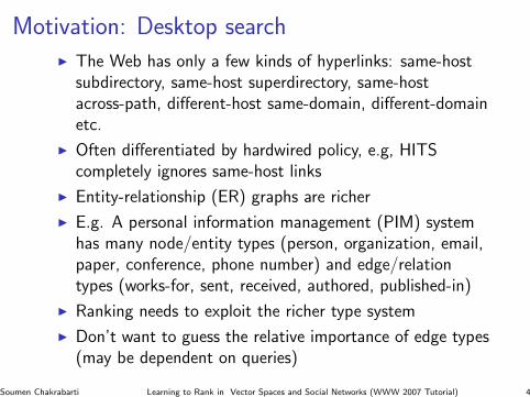
I Often differentiated by hardwired policy, e.g, HITScompletely ignores same-host links

I Entity-relationship (ER) graphs are richer

I E.g. A personal information management (PIM) systemhas many node/entity types (person, organization, email,paper, conference, phone number) and edge/relationtypes (works-for, sent, received, authored, published-in)

I Ranking needs to exploit the richer type system

I Don’t want to guess the relative importance of edge types(may be dependent on queries)


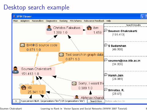
Desktop search example


Relevance feedbackI Relevance feedback is well-explored in traditional IR

I User-assisted local modification of ranking function forvector-space models

I How to extend these to richer data representations thatincorporate entities, relationship links, entity and relationtypes?

I Surprisingly unexplored area


Tutorial outline: PreliminariesI Training and evaluation scenarios

I Measurements to evaluate quality of rankingI Label mismatch loss functions for ordinal regressionI Preference pair violationsI Area under (true positive, false positive) curveI Average precisionI Rank-discounted reward for relevanceI Rank correlations

I What’s useful vs. what’s easy to learn


Tutorial outline: Ranking in vector spaces

Instance v is represented by a feature vector xv ∈ Rd

I Discriminative max-margin ranking (RankSVM)

I Linear-time max-margin approximation

I Probabilistic ranking in vector spaces (RankNet)

I Sensitivity to absolute rank and cost of poor rankings


Tutorial outline: Ranking in graphs

Instance v is a node in a graph G = (V , E )

I The graph-Laplacian approachI Assign scores to nodes to induce rankingI G imposes a smoothness constraint on node scoresI Large difference between neighboring node scores

penalized

I The Markov walk approachI Random surfer, Pagerank and variants; by far most

popular way to use graphs for scoring nodesI Walks constrained by preferencesI How to incorporate node, edge types and query words

I Surprising connections between the two approaches


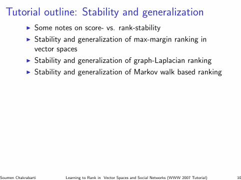
Tutorial outline: Stability and generalizationI Some notes on score- vs. rank-stability

I Stability and generalization of max-margin ranking invector spaces

I Stability and generalization of graph-Laplacian ranking

I Stability and generalization of Markov walk based ranking


Preliminaries

I MotivationI Training and evaluation setupI Performance measures

Ranking in vector spaces

I Discriminative, max-margin algorithmsI Probabilistic models, gradient-descent algorithms

Ranking nodes in graphs

I Roughness penalty using graph LaplacianI Constrained network flows

Stability and generalization

I Admissibility and stabilityI Ranking loss and generalization bounds


Preliminaries









Preliminaries









Preliminaries









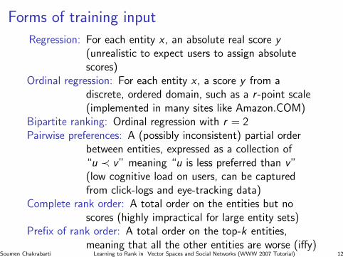
Forms of training input

Regression: For each entity x , an absolute real score y(unrealistic to expect users to assign absolutescores)

Ordinal regression: For each entity x , a score y from adiscrete, ordered domain, such as a r -point scale(implemented in many sites like Amazon.COM)

Bipartite ranking: Ordinal regression with r = 2Pairwise preferences: A (possibly inconsistent) partial order

between entities, expressed as a collection of“u ≺ v” meaning “u is less preferred than v”(low cognitive load on users, can be capturedfrom click-logs and eye-tracking data)

Complete rank order: A total order on the entities but noscores (highly impractical for large entity sets)

Prefix of rank order: A total order on the top-k entities,meaning that all the other entities are worse (iffy)


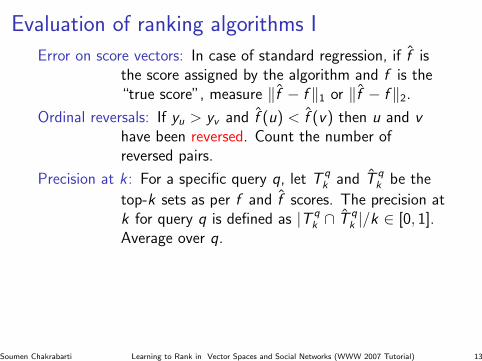
Evaluation of ranking algorithms I

Error on score vectors: In case of standard regression, if f isthe score assigned by the algorithm and f is the“true score”, measure ‖f − f ‖1 or ‖f − f ‖2.

Ordinal reversals: If yu > yv and f (u) < f (v) then u and vhave been reversed. Count the number ofreversed pairs.

Precision at k : For a specific query q, let T qk and T q

k be the

top-k sets as per f and f scores. The precision atk for query q is defined as |T q

k ∩ T qk |/k ∈ [0, 1].

Average over q.


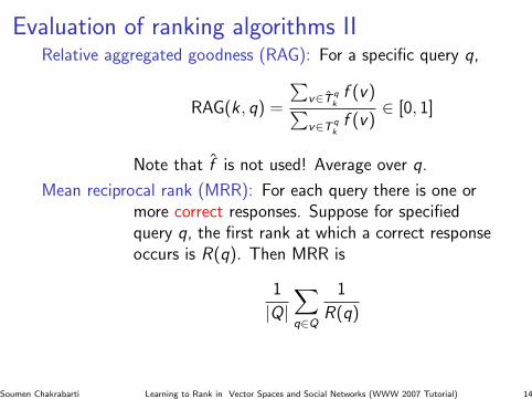
Evaluation of ranking algorithms IIRelative aggregated goodness (RAG): For a specific query q,

RAG(k , q) =

∑v∈T q

kf (v)∑

v∈T qkf (v)

∈ [0, 1]

Note that f is not used! Average over q.

Mean reciprocal rank (MRR): For each query there is one ormore correct responses. Suppose for specifiedquery q, the first rank at which a correct responseoccurs is R(q). Then MRR is

1

|Q|∑q∈Q

1

R(q)


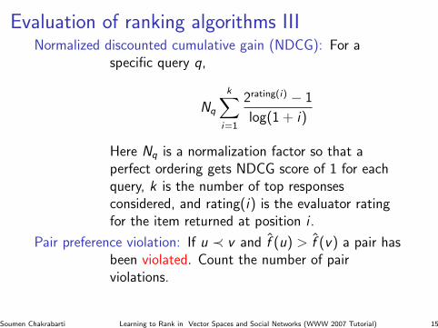
Evaluation of ranking algorithms IIINormalized discounted cumulative gain (NDCG): For a

specific query q,

Nq

k∑i=1

2rating(i) − 1

log(1 + i)

Here Nq is a normalization factor so that aperfect ordering gets NDCG score of 1 for eachquery, k is the number of top responsesconsidered, and rating(i) is the evaluator ratingfor the item returned at position i .

Pair preference violation: If u ≺ v and f (u) > f (v) a pair hasbeen violated. Count the number of pairviolations.


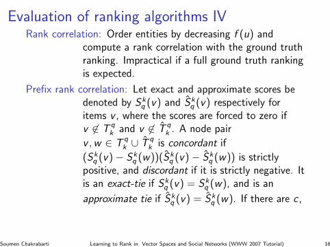
Evaluation of ranking algorithms IVRank correlation: Order entities by decreasing f (u) and

compute a rank correlation with the ground truthranking. Impractical if a full ground truth rankingis expected.

Prefix rank correlation: Let exact and approximate scores bedenoted by Sk

q (v) and Skq (v) respectively for

items v , where the scores are forced to zero ifv 6∈ T q

k and v 6∈ T qk . A node pair

v , w ∈ T qk ∪ T q

k is concordant if

(Skq (v)− Sk

q (w))(Skq (v)− Sk

q (w)) is strictlypositive, and discordant if it is strictly negative. Itis an exact-tie if Sk

q (v) = Skq (w), and is an

approximate tie if Skq (v) = Sk

q (w). If there are c ,


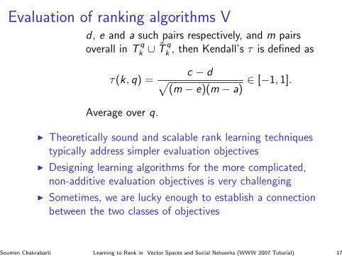
Evaluation of ranking algorithms Vd , e and a such pairs respectively, and m pairsoverall in T q

k ∪ T qk , then Kendall’s τ is defined as

τ(k , q) =c − d√

(m − e)(m − a)∈ [−1, 1].

Average over q.

I Theoretically sound and scalable rank learning techniquestypically address simpler evaluation objectives

I Designing learning algorithms for the more complicated,non-additive evaluation objectives is very challenging

I Sometimes, we are lucky enough to establish a connectionbetween the two classes of objectives


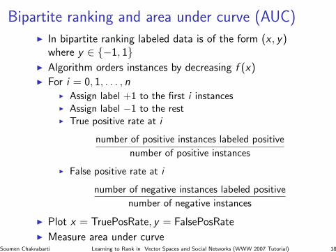
Bipartite ranking and area under curve (AUC)I In bipartite ranking labeled data is of the form (x , y)

where y ∈ −1, 1I Algorithm orders instances by decreasing f (x)I For i = 0, 1, . . . , n

I Assign label +1 to the first i instancesI Assign label −1 to the restI True positive rate at i

number of positive instances labeled positive

number of positive instances

I False positive rate at i

number of negative instances labeled positive

number of negative instances

I Plot x = TruePosRate, y = FalsePosRate

I Measure area under curveSoumen Chakrabarti Learning to Rank in Vector Spaces and Social Networks (WWW 2007 Tutorial) 18

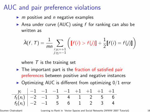
AUC and pair preference violationsI m positive and n negative examples

I Area under curve (AUC) using f for ranking can also bewritten as

A(f , T ) =1

mn

∑i :yi=+1j :yj=−1

([[f (i) > f (j)]] +

1

2[[f (i) = f (j)]]

)

where T is the training set

I The important part is the fraction of satisfied pairpreferences between positive and negative instances

I Optimizing AUC is different from optimizing 0/1 error

yi −1 −1 −1 −1 +1 +1 +1 +1f1(xi) −2 −1 3 4 1 2 5 6f2(xi) −2 −1 5 6 1 2 3 4


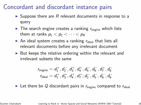
Concordant and discordant instance pairsI Suppose there are R relevant documents in response to a

query

I The search engine creates a ranking rengine which liststhem at ranks p1 < p2 < · · · < pR

I An ideal system creates a ranking rideal that lists allrelevant documents before any irrelevant document

I But keeps the relative ordering within the relevant andirrelevant subsets the same

rengine = d+1 , d−2 , d+

3 , d+4 , d−5 , d−6 , d+

7 , d−8rideal = d+

1 , d+3 , d+

4 , d+7 ; d−2 , d−5 , d−6 , d−8

I Let there be Q discordant pairs in rengine compared to rideal


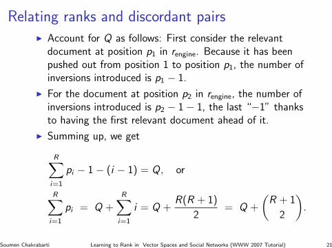
Relating ranks and discordant pairsI Account for Q as follows: First consider the relevant

document at position p1 in rengine. Because it has beenpushed out from position 1 to position p1, the number ofinversions introduced is p1 − 1.

I For the document at position p2 in rengine, the number ofinversions introduced is p2 − 1− 1, the last “−1” thanksto having the first relevant document ahead of it.

I Summing up, we get

R∑i=1

pi − 1− (i − 1) = Q, or

R∑i=1

pi = Q +R∑

i=1

i = Q +R(R + 1)

2= Q +

(R + 1

2

).


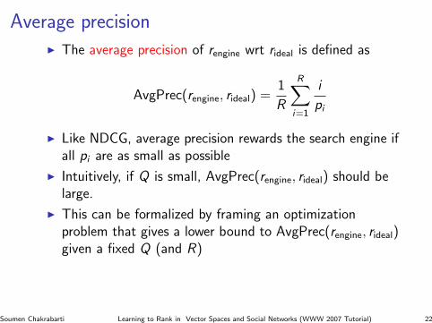
Average precisionI The average precision of rengine wrt rideal is defined as

AvgPrec(rengine, rideal) =1

R

R∑i=1

i

pi

I Like NDCG, average precision rewards the search engine ifall pi are as small as possible

I Intuitively, if Q is small, AvgPrec(rengine, rideal) should belarge.

I This can be formalized by framing an optimizationproblem that gives a lower bound to AvgPrec(rengine, rideal)given a fixed Q (and R)


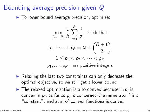
Bounding average precision given QI To lower bound average precision, optimize:

minp1,...,pR

1

R

R∑i=1

i

pisuch that

p1 + · · ·+ pR = Q +

(R + 1

2

)1 ≤ p1 < p2 < · · · < pR

p1, . . . , pR are positive integers

I Relaxing the last two constraints can only decrease theoptimal objective, so we still get a lower bound

I The relaxed optimization is also convex because 1/pi isconvex in pi , as far as pi is concerned the numerator i is a“constant”, and sum of convex functions is convex


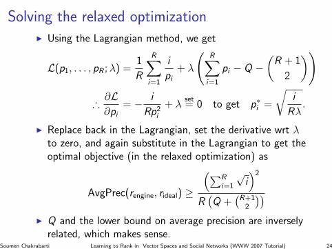
Solving the relaxed optimizationI Using the Lagrangian method, we get

L(p1, . . . , pR ; λ) =1

R

R∑i=1

i

pi+ λ

(R∑

i=1

pi − Q −(

R + 1

2

))

∴∂L∂pi

= − i

Rp2i

+ λset= 0 to get p∗i =

√i

Rλ.

I Replace back in the Lagrangian, set the derivative wrt λto zero, and again substitute in the Lagrangian to get theoptimal objective (in the relaxed optimization) as

AvgPrec(rengine, rideal) ≥

(∑Ri=1

√i)2

R(Q +

(R+1

2

))I Q and the lower bound on average precision are inversely

related, which makes sense.Soumen Chakrabarti Learning to Rank in Vector Spaces and Social Networks (WWW 2007 Tutorial) 24

Preliminaries









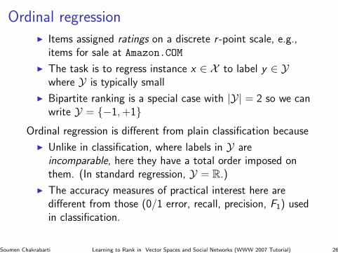
Ordinal regressionI Items assigned ratings on a discrete r -point scale, e.g.,

items for sale at Amazon.COM

I The task is to regress instance x ∈ X to label y ∈ Ywhere Y is typically small

I Bipartite ranking is a special case with |Y| = 2 so we canwrite Y = −1, +1

Ordinal regression is different from plain classification because

I Unlike in classification, where labels in Y areincomparable, here they have a total order imposed onthem. (In standard regression, Y = R.)

I The accuracy measures of practical interest here aredifferent from those (0/1 error, recall, precision, F1) usedin classification.


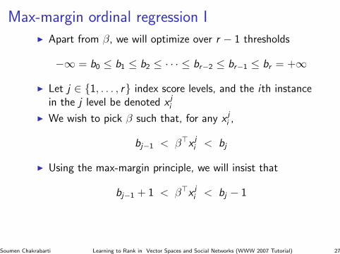
Max-margin ordinal regression II Apart from β, we will optimize over r − 1 thresholds

−∞ = b0 ≤ b1 ≤ b2 ≤ · · · ≤ br−2 ≤ br−1 ≤ br = +∞

I Let j ∈ 1, . . . , r index score levels, and the ith instancein the j level be denoted x j

i

I We wish to pick β such that, for any x ji ,

bj−1 < β>x ji < bj

I Using the max-margin principle, we will insist that

bj−1 + 1 < β>x ji < bj − 1


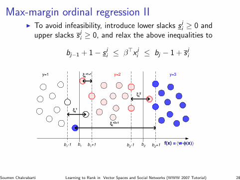
Max-margin ordinal regression III To avoid infeasibility, introduce lower slacks s j

i ≥ 0 andupper slacks s j

i ≥ 0, and relax the above inequalities to

bj−1 + 1− s ji ≤ β>x j

i ≤ bj − 1 + s jiNew Approaches to Support Vector Ordinal Regression

the thresholds, exactly as Shashua and Levin (2003)proposed, but we introduce explicit constraints in theproblem formulation that enforce the inequalities onthe thresholds. The second approach is entirely new;it considers the training samples from all the ranksto determine each threshold. Interestingly, we showthat, in this second approach, the ordinal inequalityconstraints on the thresholds are automatically satis-fied at the optimal solution though there are no ex-plicit constraints on these thresholds. For both ap-proaches the size of the optimization problems is linearin the number of training samples. We show that thepopular SMO algorithm (Platt, 1999; Keerthi et al.,2001) for SVMs can be easily adapted for the two ap-proaches. The resulting algorithms scale efficiently;empirical analysis shows that the cost is roughly aquadratic function of the problem size. Using severalbenchmark datasets we demonstrate that the gener-alization capabilities of the two approaches are muchbetter than that of the naive approach of doing stan-dard regression on the ordinal labels.

The paper is organized as follows. In section 2 wepresent the first approach with explicit inequality con-straints on the thresholds, derive the optimality con-ditions for the dual problem, and adapt the SMO al-gorithm for the solution. In section 3 we present thesecond approach with implicit constraints. In section4 we do an empirically study to show the scaling prop-erties of the two algorithms and their generalizationperformance. We conclude in section 5.

Notations Throughout this paper we will use x to de-

note the input vector of the ordinal regression problem and

φ(x) to denote the feature vector in a high dimensional re-

producing kernel Hilbert space (RKHS) related to x by

transformation. All computations will be done using the

reproducing kernel function only, which is defined as

K(x, x′) = 〈φ(x) · φ(x′)〉 (1)

where 〈·〉 denotes inner product in the RKHS. Without loss

of generality, we consider an ordinal regression problem

with r ordered categories and denote these categories as

consecutive integers Y = 1, 2, . . . , r to keep the known

ordering information. In the j-th category, where j ∈ Y ,

the number of training samples is denoted as nj , and the

i-th training sample is denoted as xji where x

ji ∈ R

d. The

total number of training samples∑r

j=1nj is denoted as n.

bj , j = 1, . . . , r − 1 denote the (r − 1) thresholds.

2. Explicit Constraints on Thresholds

As a powerful computational tool for supervised learn-ing, support vector machines (SVMs) map the in-put vectors into feature vectors in a high dimensional

b2

b1

y=1 y=2 y=3

b2-1 b

2+1b

1-1 b

1+1

ξi∗1+1

ξi2

ξi∗2+1

ξi1

f(x) = w φ(x).

Figure 1. An illustration of the definition of slack variablesξ and ξ∗ for the thresholds. The samples from differentranks, represented as circles filled with different patterns,are mapped by 〈w · φ(x)〉 onto the axis of function value.Note that a sample from rank j +1 could be counted twicefor errors if it is sandwiched by bj+1 − 1 and bj + 1 wherebj+1 − 1 < bj + 1, and the samples from rank j + 2, j − 1etc. never give contributions to the threshold bj .

RKHS (Vapnik, 1995; Scholkopf & Smola, 2002),where a linear machine is constructed by minimizinga regularized functional. For binary classification (aspecial case of ordinal regression with r = 2), SVMsfind an optimal direction that maps the feature vec-tors into function values on the real line, and a singleoptimized threshold is used to divide the real line intotwo regions for the two classes respectively. In thesetting of ordinal regression, the support vector for-mulation could attempt to find an optimal mappingdirection w, and r − 1 thresholds, which define r − 1parallel discriminant hyperplanes for the r ranks ac-cordingly. For each threshold bj , Shashua and Levin(2003) suggested considering the samples from the twoadjacent categories, j and j + 1, for empirical errors(see Figure 1 for an illustration). More exactly, eachsample in the j-th category should have a functionvalue that is less than the lower margin bj − 1, oth-

erwise 〈w · φ(xj

i )〉 − (bj − 1) is the error (denoted as

ξj

i ); similarly, each sample from the (j+1)-th categoryshould have a function value that is greater than theupper margin bj +1, otherwise (bj +1)−〈w ·φ(xj+1

i )〉

is the error (denoted as ξ∗j+1

i ).1 Shashua and Levin(2003) generalized the primal problem of SVMs to or-dinal regression as follows:

minw,b,ξ,ξ∗

1

2〈w ·w〉+ C

r−1∑

j=1

( nj

∑

i=1

ξj

i +

nj+1

∑

i=1

ξ∗j+1

i

)

(2)

subject to

〈w · φ(xj

i )〉 − bj ≤ −1 + ξj

i ,

ξj

i ≥ 0, for i = 1, . . . , nj ;

〈w · φ(xj+1

i )〉 − bj ≥ +1− ξ∗j+1

i ,

ξ∗j+1

i ≥ 0, for i = 1, . . . , nj+1;

(3)

where j runs over 1, . . . , r − 1 and C > 0.

1The superscript ∗ in ξ∗j+1

i denotes that the error isassociated with a sample in the adjacent upper category ofthe j-th threshold.


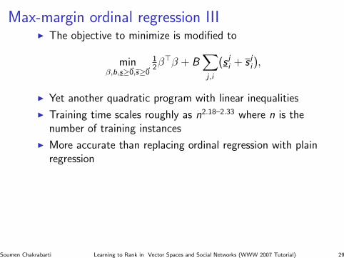
Max-margin ordinal regression IIII The objective to minimize is modified to

minβ,b,s≥~0,s≥~0

12β>β + B

∑j ,i

(s ji + s j

i ),

I Yet another quadratic program with linear inequalities

I Training time scales roughly as n2.18–2.33 where n is thenumber of training instances

I More accurate than replacing ordinal regression with plainregression


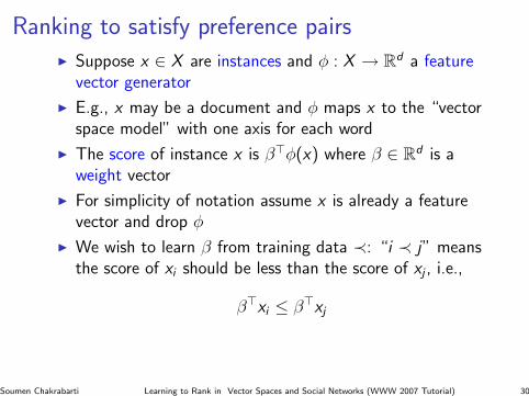
Ranking to satisfy preference pairsI Suppose x ∈ X are instances and φ : X → Rd a feature

vector generator

I E.g., x may be a document and φ maps x to the “vectorspace model” with one axis for each word

I The score of instance x is β>φ(x) where β ∈ Rd is aweight vector

I For simplicity of notation assume x is already a featurevector and drop φ

I We wish to learn β from training data ≺: “i ≺ j” meansthe score of xi should be less than the score of xj , i.e.,

β>xi ≤ β>xj


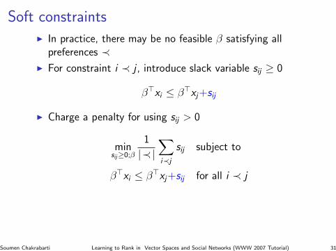
Soft constraintsI In practice, there may be no feasible β satisfying all

preferences ≺I For constraint i ≺ j , introduce slack variable sij ≥ 0

β>xi ≤ β>xj+sij

I Charge a penalty for using sij > 0

minsij≥0;β

1

|≺|∑i≺j

sij subject to

β>xi ≤ β>xj+sij for all i ≺ j


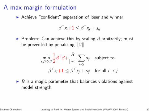
A max-margin formulationI Achieve “confident” separation of loser and winner:

β>xi+1 ≤ β>xj + sij

I Problem: Can achieve this by scaling β arbitrarily; mustbe prevented by penalizing ‖β‖

minsij≥0;β

1

2β>β+

B

|≺|∑i≺j

sij subject to

β>xi+1 ≤ β>xj + sij for all i ≺ j

I B is a magic parameter that balances violations againstmodel strength


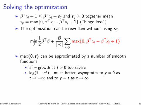
Solving the optimizationI β>xi + 1 ≤ β>xj + sij and sij ≥ 0 together mean

sij = max0, β>xi − β>xj + 1 (“hinge loss”)

I The optimization can be rewritten without using sij

minβ

1

2β>β +

B

|≺|∑i≺j

max0, β>xi − β>xj + 1

I max0, t can be approximated by a number of smoothfunctions

I et – growth at t > 0 too severeI log(1 + et) – much better, asymptotes to y = 0 as

t → −∞ and to y = t as t →∞


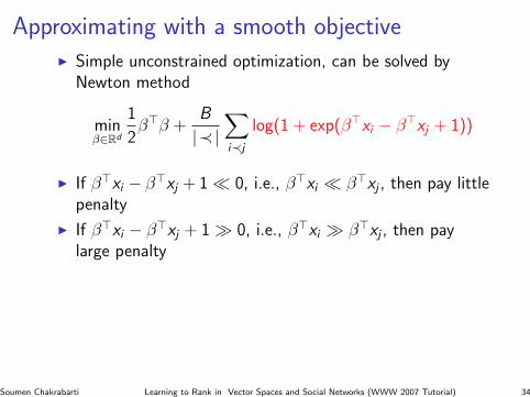
Approximating with a smooth objectiveI Simple unconstrained optimization, can be solved by

Newton method

minβ∈Rd

1

2β>β +

B

|≺|∑i≺j

log(1 + exp(β>xi − β>xj + 1))

I If β>xi − β>xj + 1 0, i.e., β>xi β>xj , then pay littlepenalty

I If β>xi − β>xj + 1 0, i.e., β>xi β>xj , then paylarge penalty


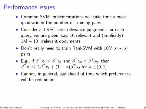
Performance issuesI Common SVM implementations will take time almost

quadratic in the number of training pairs

I Consider a TREC-style relevance judgment: for eachquery, we are given, say, 10 relevant and (implicitly)1M− 10 irrelevant documents

I Don’t really need to train RankSVM with 10M xi ≺ xj

pairs

I E.g., if β>x0 ≤ β>x1 and β>x0 ≤ β>x2, thenβ>x0 ≤ λβ>x1 + (1− λ)β>x2 for λ ∈ [0, 1]

I Cannot, in general, say ahead of time which preferenceswill be redundant


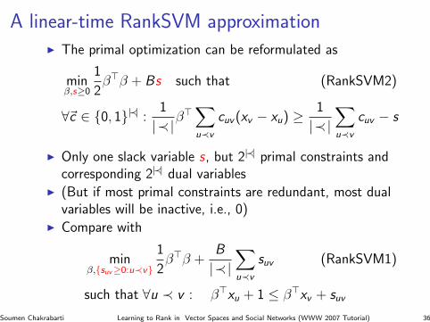
A linear-time RankSVM approximationI The primal optimization can be reformulated as

minβ,s≥0

1

2β>β + Bs such that (RankSVM2)

∀~c ∈ 0, 1|≺| : 1

|≺|β>∑u≺v

cuv(xv − xu) ≥1

|≺|∑u≺v

cuv − s

I Only one slack variable s, but 2|≺| primal constraints andcorresponding 2|≺| dual variables

I (But if most primal constraints are redundant, most dualvariables will be inactive, i.e., 0)

I Compare with

minβ,suv≥0:u≺v

1

2β>β +

B

|≺|∑u≺v

suv (RankSVM1)

such that ∀u ≺ v : β>xu + 1 ≤ β>xv + suv


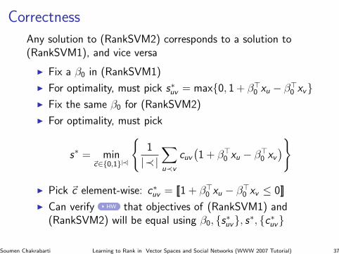
Correctness

Any solution to (RankSVM2) corresponds to a solution to(RankSVM1), and vice versa

I Fix a β0 in (RankSVM1)

I For optimality, must pick s∗uv = max0, 1 + β>0 xu − β>0 xvI Fix the same β0 for (RankSVM2)

I For optimality, must pick

s∗ = min~c∈0,1|≺|

1

|≺|∑u≺v

cuv

(1 + β>0 xu − β>0 xv

)

I Pick ~c element-wise: c∗uv = [[1 + β>0 xu − β>0 xv ≤ 0]]

I Can verify HW that objectives of (RankSVM1) and(RankSVM2) will be equal using β0, s∗uv, s∗, c∗uv


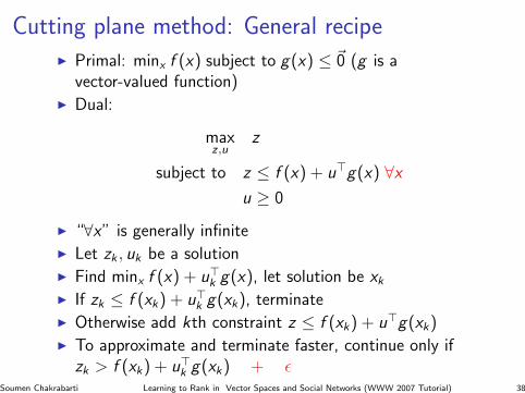
Cutting plane method: General recipeI Primal: minx f (x) subject to g(x) ≤ ~0 (g is a

vector-valued function)I Dual:

maxz,u

z

subject to z ≤ f (x) + u>g(x) ∀xu ≥ 0

I “∀x” is generally infiniteI Let zk , uk be a solutionI Find minx f (x) + u>k g(x), let solution be xk

I If zk ≤ f (xk) + u>k g(xk), terminateI Otherwise add kth constraint z ≤ f (xk) + u>g(xk)I To approximate and terminate faster, continue only if

zk > f (xk) + u>k g(xk) + εSoumen Chakrabarti Learning to Rank in Vector Spaces and Social Networks (WWW 2007 Tutorial) 38

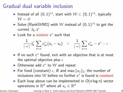
Gradual dual variable inclusionI Instead of all 0, 1|≺|, start with W ⊂ 0, 1|≺|, typicallyW = ∅

I Solve (RankSVM2) with W instead of 0, 1|≺| to get thecurrent β0, s

∗

I Look for a violator c∗ such that

1

|≺|β>0∑u≺v

c∗uv(xv − xu) <1

|≺|∑u≺v

c∗uv − s∗ − ε

I If no such c∗ found, exit with an objective that is at mostthe optimal objective plus ε

I Otherwise add c∗ to W and repeatI For fixed (constant) ε, B and max ‖xv‖2, the number of

inclusions into W before no further c∗ is found is constantI Each loop above can be implemented in O(n log n) vector

operations in Rd where all xv ∈ Rd


Linear-time (RankSVM2) performance

I Almost linear scaling inpractice too

I Dramatic improvementover (RankSVM1)

I (RankSVM1) scalesroughly as n3.4 (notshown)

SVM-Perf (Classification) SVM-Light (Classification) SVM-Perf (Class. opt. C) SVM-Perf (Ord. Regr.)

0.1

1

10

100

1000

10000

100000

100 1000 10000 100000 1e+06

CP

U-S

eco

nd

s

Number of Training Examples

Reuters CCATReuters C11

Arxiv astro-phCovertype 1

KDD04 PhysicsO(x^0.8)

0.1

1

10

100

1000

10000

100000

100 1000 10000 100000 1e+06

CP

U-S

eco

nd

s





0.1

1

10

100

1000

10000

100000

100 1000 10000 100000 1e+06

CP

U-S

eco

nd

s





0.1

1

10

100

1000

10000

100000

100 1000 10000 100000 1e+06C

PU

-Se

co

nd

s





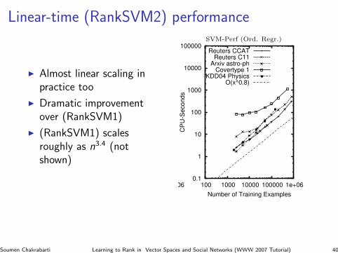
Figure 1: Training time of SVM-Perf (left) and SVM-Light (left-middle) for classification as a function of n

for the value of C that gives best test set performance for the maximum training set size. The middle-rightplot shows training time of SVM-Perf for the value of C with optimum test set performance for the respectivetraining set size. The right-most plot is the CPU-time of SVM-Perf for ordinal regression.

how L2-SVM-MFN scales. In the worst case, the authorsconclude that each iteration may scale O(sn minn, N), al-though practical scaling is likely to be substantially better.Finally, note that L2-SVM-MFN uses squared slack vari-ables

ξ2

i to measure training loss instead of linear slacksξi like in SVM-Light and SVM-Perf.The Lagrangian SVM (LSVM) [18] is another method par-

ticularly suited for training linear SVMs. Like the L2-SVM-MFN, the LSVM uses squared slack variables

ξ2

i to mea-sure training loss. The LSVM can be very fast if the numberof features N is small, scaling roughly as O(nN2). We ap-plied the implementation of Mangasarian and Musicant3 tothe Adult and the Web data using the values of C from above.With 31.4 CPU-seconds, the training time of the LSVM isstill comparable on Adult. For the higher-dimensional Webtask, the LSVM runs into convergence problems. Apply-ing the LSVM to tasks with thousands of features is nottractable, since the algorithm requires storing and invertingan N ×N matrix.

4.2 How does Training Time Scale with theNumber of Training Examples?

Figure 1 shows log-log plots of how CPU-time increaseswith the size of the training set. The left-most plot shows thescaling of SVM-Perf for classification, while the left-middleplot shows the scaling of SVM-Light. Lines in a log-logplot correspond to polynomial growth O(nd), where d cor-responds to the slope of the line. The middle plot showsthat SVM-Light scales roughly O(n1.7), which is consistentwith previous observations [11]. SVM-Perf has much betterscaling, which is (to some surprise) better than linear withroughly O(n0.8) over much of the range.

Figure 2 gives insight into the reason for this scaling be-havior. The graph shows the number of iterations of SVM-Perf (and therefore the maximum number of constraints inthe working set) in relation to the training set size n. Itturns out that the number of iterations is not only upperbounded independent of n as shown in Lemma 2, but that

3http://www.cs.wisc.edu/dmi/lsvm/

1

10

100

1000

1000 10000 100000 1e+06

Ite

ratio

ns




KDD04 Physics

Figure 2: Number of iterations of SVM-Perf for clas-sification as a function of sample size n.

it does not grow with n even in the non-asymptotic region.In fact, for some of the problems the number of iterationsdecreases with n, which explains the sub-linear scaling inCPU-time. Another explanation lies in the high “fixed cost”that is independent of n, which is mostly the cost for solvinga quadratic program in each iteration.

Since Lemma 2 identifies that the number of iterationsdepends on the value of C, scaling for the optimal value ofC might be different if the optimal C increases with trainingset size. To analyze this, the middle-right plot of Figure 1shows training time for the optimal value of C. While thecurves look more noisy, the scaling still seems to be roughlylinear.

Finally, the right-most plot in Figure 1 shows trainingtime of SVM-Perf for ordinal regression. The scaling isslightly steeper than for classification as expected. The num-ber of iterations is virtually identical to the case of classifi-cation shown in Figure 2. Note that training time of SVM-Light would scale roughly O(n3.4) on this problem.


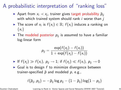
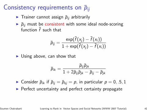
A probabilistic interpretation of “ranking loss”I Apart from xi ≺ xj , trainer gives target probability pij

with which trained system should rank i worse than j

I The score of xi is f (xi) ∈ R; f (xi) induces a ranking onxi

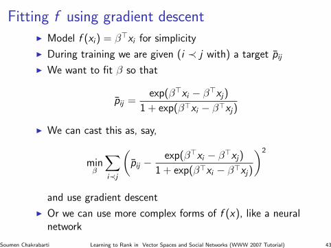
I The modeled posterior pij is assumed to have a familiarlog-linear form

pij =exp(f (xj)− f (xi))

1 + exp(f (xj)− f (xi))

I If f (xj) f (xi), pij → 1; if f (xj) f (xi), pij → 0

I Goal is to design f to minimize divergence betweentrainer-specified p and modeled p, e.g.,

`(pij , pij) = −pij log pij − (1− pij) log(1− pij)


Consistency requirements on pij

I Trainer cannot assign pij arbitrarily

I pij must be consistent with some ideal node-scoringfunction f such that

pij =exp(f (xj)− f (xi))

1 + exp(f (xj)− f (xi))

I Using above, can show that

pik =pij pjk

1 + 2pij pjk − pij − pjk

I Consider pik if pij = pkj = p, in particular p = 0, .5, 1

I Perfect uncertainty and perfect certainty propagate


Fitting f using gradient descentI Model f (xi) = β>xi for simplicity

I During training we are given (i ≺ j with) a target pij

I We want to fit β so that

pij =exp(β>xi − β>xj)

1 + exp(β>xi − β>xj)

I We can cast this as, say,

minβ

∑i≺j

(pij −

exp(β>xi − β>xj)

1 + exp(β>xi − β>xj)

)2

and use gradient descent

I Or we can use more complex forms of f (x), like a neuralnetwork


RankBoostI Given partial orders with preference strengths φ(i , j) ≥ 0:

if positive, i j , otherwise impartial

I Input pair distribution D over X × XI Weak learner indexed by t gets input pairs as per a

distribution Dt and outputs a weak ranking ht : X → RI Initialize D1 = DI For t = 1, . . . , T

I Train tth weak learner using Dt

I Get weak ranking ht : X → RI Choose αt ∈ RI Update

Dt+1(xi , xj) ∝ Dt(xi , xj) exp(αt(ht(xi )− ht(xj))

)I Final scoring function H(x) =

∑Tt=1 αtht(x)


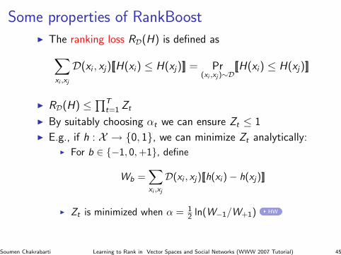
Some properties of RankBoostI The ranking loss RD(H) is defined as∑

xi ,xj

D(xi , xj)[[H(xi) ≤ H(xj)]] = Pr(xi ,xj )∼D

[[H(xi) ≤ H(xj)]]

I RD(H) ≤∏T

t=1 Zt

I By suitably choosing αt we can ensure Zt ≤ 1

I E.g., if h : X → 0, 1, we can minimize Zt analytically:I For b ∈ −1, 0,+1, define

Wb =∑xi ,xj

D(xi , xj)[[h(xi )− h(xj)]]

I Zt is minimized when α = 12 ln(W−1/W+1) HW


Preliminaries









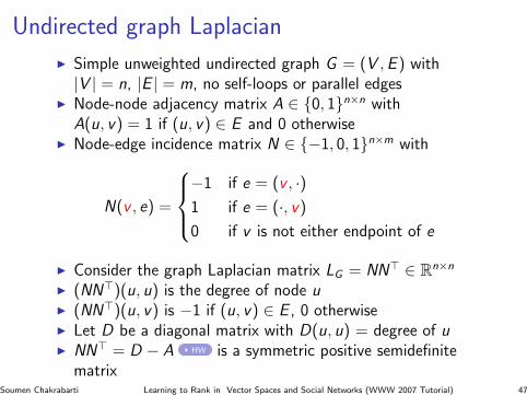
Undirected graph Laplacian

I Simple unweighted undirected graph G = (V , E ) with|V | = n, |E | = m, no self-loops or parallel edges

I Node-node adjacency matrix A ∈ 0, 1n×n withA(u, v) = 1 if (u, v) ∈ E and 0 otherwise

I Node-edge incidence matrix N ∈ −1, 0, 1n×m with

N(v , e) =

−1 if e = (v , ·)1 if e = (·, v)

0 if v is not either endpoint of e

I Consider the graph Laplacian matrix LG = NN> ∈ Rn×n

I (NN>)(u, u) is the degree of node uI (NN>)(u, v) is −1 if (u, v) ∈ E , 0 otherwiseI Let D be a diagonal matrix with D(u, u) = degree of uI NN> = D − A HW is a symmetric positive semidefinite

matrixSoumen Chakrabarti Learning to Rank in Vector Spaces and Social Networks (WWW 2007 Tutorial) 47

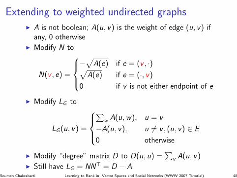
Extending to weighted undirected graphsI A is not boolean; A(u, v) is the weight of edge (u, v) if

any, 0 otherwiseI Modify N to

N(v , e) =

−√

A(e) if e = (v , ·)√A(e) if e = (·, v)

0 if v is not either endpoint of e

I Modify LG to

LG (u, v) =

∑

w A(u, w), u = v

−A(u, v), u 6= v , (u, v) ∈ E

0 otherwise

I Modify “degree” matrix D to D(u, u) =∑

v A(u, v)I Still have LG = NN> = D − A


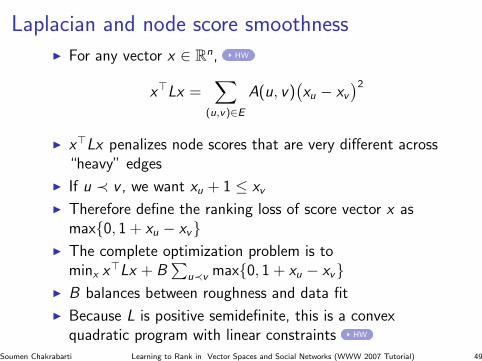
Laplacian and node score smoothnessI For any vector x ∈ Rn, HW

x>Lx =∑

(u,v)∈E

A(u, v)(xu − xv

)2I x>Lx penalizes node scores that are very different across

“heavy” edges

I If u ≺ v , we want xu + 1 ≤ xv

I Therefore define the ranking loss of score vector x asmax0, 1 + xu − xv

I The complete optimization problem is tominx x>Lx + B

∑u≺v max0, 1 + xu − xv

I B balances between roughness and data fit

I Because L is positive semidefinite, this is a convexquadratic program with linear constraints HW


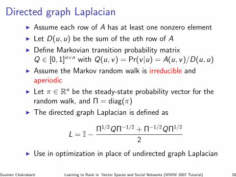
Directed graph LaplacianI Assume each row of A has at least one nonzero element

I Let D(u, u) be the sum of the uth row of A

I Define Markovian transition probability matrixQ ∈ [0, 1]n×n with Q(u, v) = Pr(v |u) = A(u, v)/D(u, u)

I Assume the Markov random walk is irreducible andaperiodic

I Let π ∈ Rn be the steady-state probability vector for therandom walk, and Π = diag(π)

I The directed graph Laplacian is defined as

L = I− Π1/2QΠ−1/2 + Π−1/2QΠ1/2

2

I Use in optimization in place of undirected graph Laplacian


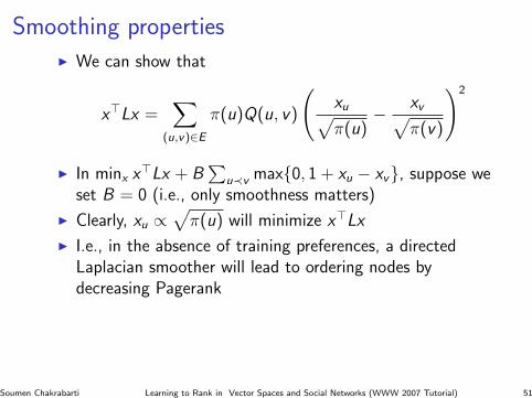
Smoothing propertiesI We can show that

x>Lx =∑

(u,v)∈E

π(u)Q(u, v)

(xu√π(u)

− xv√π(v)

)2

I In minx x>Lx + B∑

u≺v max0, 1 + xu − xv, suppose weset B = 0 (i.e., only smoothness matters)

I Clearly, xu ∝√

π(u) will minimize x>Lx

I I.e., in the absence of training preferences, a directedLaplacian smoother will lead to ordering nodes bydecreasing Pagerank


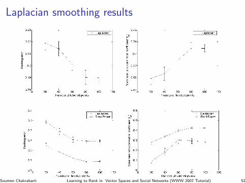
Laplacian smoothing resultsRanking on Graph Data

Figure 2. Performance of our algorithm on the 5-partite b.1.1.1 protein ranking task. Left: Ranking error (test set). Right: Spearman

rank-order correlation (test set). Each point is an average over 10 random splits; error bars show standard error. (See text for details.)

The SCOP/PSI-BLAST data set2 consists of (dis)similarity

scores between pairs of SCOP proteins, computed using the

popular PSI-BLAST sequence search and alignment tool

(Altschul et al., 1997). This data set has been used in an-

other kind of protein ranking task in (Weston et al., 2004)3.

In our experiments, we used a subset of the SCOP data con-

sisting of 3314 proteins from two classes (all alpha and all

beta). Following (Weston et al., 2004), we converted the

dissimilarity scores (E-values returned by PSI-BLAST) to

similarity scores by taking w(vi, vj) = exp(−Eij/100),where Eij denotes the E-value assigned by PSI-BLAST to

protein vj given query vi. The similarity scores were then

used to define a weighted data graph over the 3314 proteins.

The scores are actually asymmetric; consequently, the data

graph G in this case was a directed graph.

We took the largest protein family data set (an all beta fam-

ily of V set domains (antibody variable like), denoted as

b.1.1.1 in the data set, consisting of 403 proteins) as our

target, and evaluated our algorithm on the ranking task as-

sociated with this family. The ranking task was defined as

described above, with τ(vi, vj) =(

level(j) − level(i))

+.

We used our Laplacian-based ranking algorithm from Sec-

tion 4; in constructing the graph Laplacian, we used a tele-

porting random walk with η = 0.01 (see Section 4).

The results are shown in Figure 2. Experiments were con-

ducted with varying numbers of labeled examples; the re-

sults for each number are averaged over 10 trials (random

train/test splits, subject to a fixed proportion of proteins

from the 5 rank levels). Error bars show standard error. For

each train/test split, the order graph consisted of the appro-

2Available at www.kyb.tuebingen.mpg.de/bs/people/weston/rankprot/supplement.html

3Again, it is important to note that the ranking problem in(Weston et al., 2004), as in (Zhou et al., 2004), is very differ-ent from those considered in this paper; in particular, the rankingtasks there are defined by a single protein as a query, and cannotbe formulated within our order graph setting.

priate τ values for edges within the training set; a similar

order graph over the test set was used to compute the rank-

ing error plotted in the first graph. We also computed in

each case the Spearman rank-order correlation between the

“true” ranking of the test proteins (ranks between 1 and 5)

and the learned ranking; this is plotted in the second graph.

The value of the parameter C in the algorithm was selected

from the set 0.01, 0.1, 1, 10, 100 using 5-fold cross vali-

dation in each trial; to compensate for the small training set

sizes, the cross-validation was done by dividing the training

edges into 5 groups, rather than the vertices.

The above protein ranking task is an example of a ranking

problem which, due to the graph-based input data repre-

sentation, could not be tackled using previous approaches.

In order to compare our approach to others, we used next

a data set in which the data could be represented both as

vector data and as graph data.

6.2. Document Ranking – 20 Newsgroups Data

The 20 newsgroups data set4 consists of documents com-

prised of newsgroup messages, classified according to

newsgroup. We used the “mini” version of the data set in

our experiments, which contains a total of 2000 messages,

100 each from 20 different newsgroups. These newsgroups

can be grouped together into categories based on subject

matter, allowing for a hierarchical classification. This again

leads to a natural ranking task associated with any target

newsgroup: messages from the given newsgroup are to be

ranked highest (level 1), followed by messages from other

newsgroups in the same category (level 2), followed fi-

nally by messages in other categories (level 3). This can

be viewed as a 3-partite ranking task.

We categorized the 20 newsgroups according to the

recommendation given by Jason Rennie on his webpage,

4Available at www.ics.uci.edu/ kdd/databases/20newsgroups/20newsgroups.html

30

Ranking on Graph Data

Figure 3. Comparison of our algorithm with RankBoost on the 3-partite alt.atheism newsgroup document ranking task. Left: Ranking

error (test set). Right: Spearman rank-order correlation (test set). Each point is an average over 10 random splits; error bars show

standard error. (See text for details.)

http://people.csail.mit.edu/jrennie/20Newsgroups/, and

chose the alt.atheism newsgroup as our target. There were

two other newsgroups in the same category as the target,

namely soc.religion.christian and talk.religion.misc.

Following (Belkin & Niyogi, 2004), we tokenized the doc-

uments using the Rainbow software package written by An-

drew McCallum, using a stop list of approximately 500

common words and removing message headers. The vector

representation of each message then consisted of the counts

of the most frequent 6000 words, normalized so as to sum

to 1. The graph representation of the data was derived from

the vector values; in particular, we constructed an undi-

rected graph over the 2000 documents using Gaussian sim-

ilarity weights given by w(vi, vj) = exp(−||xi − xj ||2),

where xi denotes the vector representation of document vi.

We applied our Laplacian-based ranking algorithm from

Section 3, and compared this to the RankBoost algorithm

of (Freund et al., 2003), using threshold rankers with range

0, 1 (similar to boosted stumps) as weak rankings.

The results are shown in Figure 3. The results for each

number are averaged over 10 trials (random train/test splits,

subject to equal numbers from all newsgroups). RankBoost

was run for 100 rounds in each trial (increasing the number

of rounds further did not yield any improvement in perfor-

mance). Similarly to the protein ranking experiments, the

value of the parameter C in each trial was selected from the

set 0.01, 0.1, 1, 10, 100 using 4-fold cross validation.

It should be noted that this is not truly a fair comparison,

since RankBoost operates in a strictly supervised setting,

i.e., it sees only the training points, while the Laplacian

algorithm operates in a transductive setting and sees the

complete data graph. What it shows, however, is that for

domains in which ranking labels are limited but similarity

information about data points can be obtained, one can gain

considerably by using an algorithm that can exploit this in-

formation.

7. Discussion

The goal of this paper has been to extend the growing

repertoire of ranking algorithms to data represented in the

form of a (similarity) graph. Building on recent develop-

ments in regularization theory for graphs and correspond-

ing Laplacian-based methods for classification, we have

developed an algorithmic framework for learning ranking

functions on both undirected and directed graphs.

Our algorithms have an SVM-like flavour in their formu-

lations; indeed, they can be viewed as minimizing a reg-

ularized ranking error within a reproducing kernel Hilbert

space (RKHS). From a theoretical standpoint, this means

that they benefit from theoretical results such as those es-

tablishing stability and generalization properties of algo-

rithms that perform regularization within an RKHS. From

a practical standpoint, it means that the implementation of

these algorithms can benefit from the large variety of tech-

niques that have been developed for scaling SVMs to large

data sets (e.g., (Joachims, 1999; Platt, 1999)).

The formulation of the graph ranking problem that we have

focused on in this paper falls under the setting of transduc-

tive learning. It should be possible to use out-of-sample

extension techniques, such as those of (Sindhwani et al.,

2005), to extend our framework to a semi-supervised learn-

ing setting.

Acknowledgments

The author would like to thank Partha Niyogi for stimu-

lating discussions on many topics related to this work, in-

cluding manifold and graph Laplacians and regularization

theory for continuous and discrete spaces; these discus-

sions took place mostly at the Chicago Machine Learning

Summer School in May 2005. The author also benefited

from a lecture by Fan Chung in the MIT Applied Mathe-

31


Limitations of the graph Laplacian approachI The “link as hint of score smoothness” view is not

universally applicable: millions of obscure pages u link tov =http://yahoo.com, with xu xv

I While π(u) is a probability, xu ∈ R is an arbitrary scorethat need not satisfy Markov balance constraints (comingsoon) and may even be negative

I Dual optimization involves computing the pseudoinverseL+ of the Laplacian matrix

I Unlike L, L+ is usually not sparse, and most packagesneed to hold it in RAM

I The generalization power of the learner (defined later)depends on κ = maxu∈V L+(u, u), a quantity hard tointerpret


http://yahoo.com

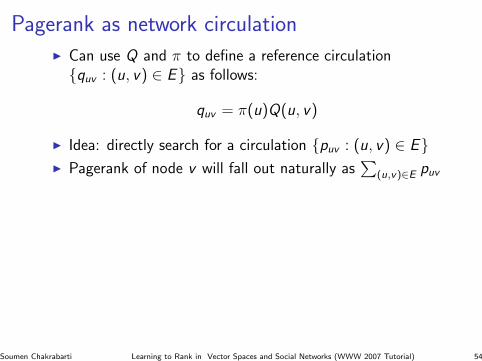
Pagerank as network circulationI Can use Q and π to define a reference circulationquv : (u, v) ∈ E as follows:

quv = π(u)Q(u, v)

I Idea: directly search for a circulation puv : (u, v) ∈ EI Pagerank of node v will fall out naturally as

∑(u,v)∈E puv


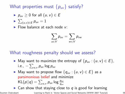
What properties must puv satisfy?

I puv ≥ 0 for all (u, v) ∈ E

I∑

(u,v)∈E puv = 1

I Flow balance at each node v :∑u∈V

puv =∑w∈V

pvw

What roughness penalty should we assess?

I May want to maximize the entropy of puv : (u, v) ∈ E,i.e., −

∑u,v puv log puv

I May want to propose flow quv : (u, v) ∈ E as aparsimonious belief and minimizeKL(p||q) =

∑u,v puv log puv

quv

I Can show that staying close to q is good for learningSoumen Chakrabarti Learning to Rank in Vector Spaces and Social Networks (WWW 2007 Tutorial) 55

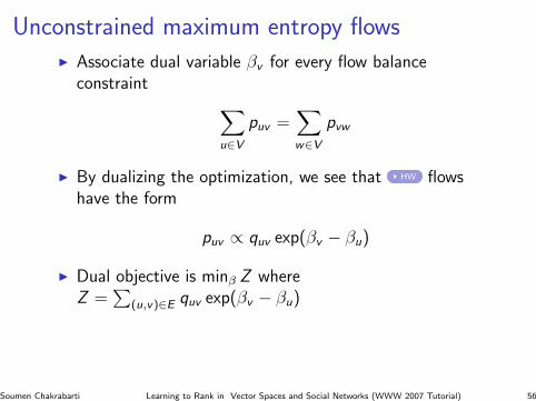
Unconstrained maximum entropy flowsI Associate dual variable βv for every flow balance

constraint ∑u∈V

puv =∑w∈V

pvw

I By dualizing the optimization, we see that HW flowshave the form

puv ∝ quv exp(βv − βu)

I Dual objective is minβ Z whereZ =

∑(u,v)∈E quv exp(βv − βu)


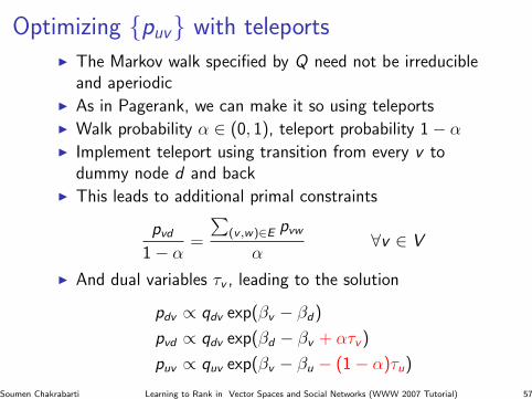
Optimizing puv with teleportsI The Markov walk specified by Q need not be irreducible

and aperiodicI As in Pagerank, we can make it so using teleportsI Walk probability α ∈ (0, 1), teleport probability 1− αI Implement teleport using transition from every v to

dummy node d and backI This leads to additional primal constraints

pvd

1− α=

∑(v ,w)∈E pvw

α∀v ∈ V

I And dual variables τv , leading to the solution

pdv ∝ qdv exp(βv − βd)

pvd ∝ qdv exp(βd − βv + ατv)

puv ∝ quv exp(βv − βu − (1− α)τu)


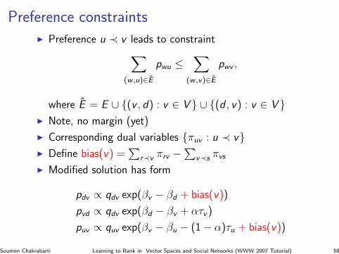
Preference constraintsI Preference u ≺ v leads to constraint∑

(w ,u)∈E

pwu ≤∑

(w ,v)∈E

pwv ,

where E = E ∪ (v , d) : v ∈ V ∪ (d , v) : v ∈ V I Note, no margin (yet)

I Corresponding dual variables πuv : u ≺ vI Define bias(v) =

∑r≺v πrv −

∑v≺s πvs

I Modified solution has form

pdv ∝ qdv exp(βv − βd + bias(v))

pvd ∝ qdv exp(βd − βv + ατv)

puv ∝ quv exp(βv − βu − (1− α)τu + bias(v))


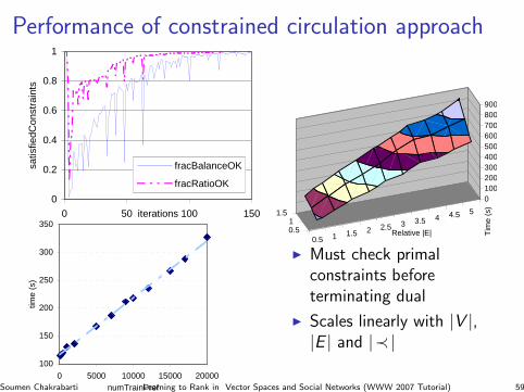
Performance of constrained circulation approach

0

0.2

0.4

0.6

0.8

1

0 50 100 150iterations

satis

fiedC

onst

rain

ts

fracBalanceOK

fracRatioOK

100

150

200

250

300

350

0 5000 10000 15000 20000numTrainPref

time

(s)

0.5 1 1.5 2 2.5 3 3.5 4 4.5 5

0.51

1.5

0100200300400500600700800900

Tim

e (s

)

Relative |E|

I Must check primalconstraints beforeterminating dual

I Scales linearly with |V |,|E | and |≺|


Incorporating an additive marginI Preference constraints were expressed as∑

(w ,u)∈E pwu ≤∑

(w ,v)∈E pwv , not

1 +∑

(w ,u)∈E pwu ≤ suv +∑

(w ,v)∈E pwv

I suv ≥ 0 is a primal slack variableI Because

∑u,v puv = 1, 1 is “too aggressive” as a margin

I . . . unless we scale up puvI Let q be a probability distribution and p an unnormalized

distribution such that∑

x p(x) = FI KL(p‖q) ≥ 0 if F ≥ 1I For a fixed F ≥ 1, arg minp KL(p‖q) = Fq

I New objective

minpuv,suv≥0,F≥1

KL(p‖q) + C∑u≺v

suv + C1F2

I New constraint∑

u,v puv = F replaces∑

u,v puv = 1


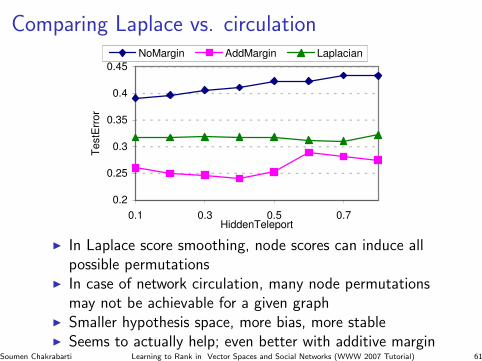
Comparing Laplace vs. circulation

0.2

0.25

0.3

0.35

0.4

0.45

0.1 0.3 0.5 0.7HiddenTeleport

TestE

rror

NoMargin AddMargin Laplacian

I In Laplace score smoothing, node scores can induce allpossible permutations

I In case of network circulation, many node permutationsmay not be achievable for a given graph

I Smaller hypothesis space, more bias, more stableI Seems to actually help; even better with additive margin


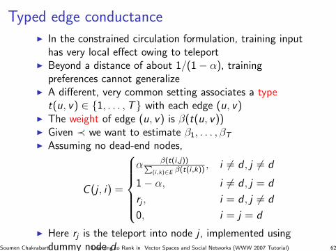
Typed edge conductanceI In the constrained circulation formulation, training input

has very local effect owing to teleportI Beyond a distance of about 1/(1− α), training

preferences cannot generalizeI A different, very common setting associates a type

t(u, v) ∈ 1, . . . , T with each edge (u, v)I The weight of edge (u, v) is β(t(u, v))I Given ≺ we want to estimate β1, . . . , βT

I Assuming no dead-end nodes,

C (j , i) =

α β(t(i ,j))P

(i,k)∈E β(t(i ,k)), i 6= d , j 6= d

1− α, i 6= d , j = d

rj , i = d , j 6= d

0, i = j = d

I Here rj is the teleport into node j , implemented usingdummy node dSoumen Chakrabarti Learning to Rank in Vector Spaces and Social Networks (WWW 2007 Tutorial) 62

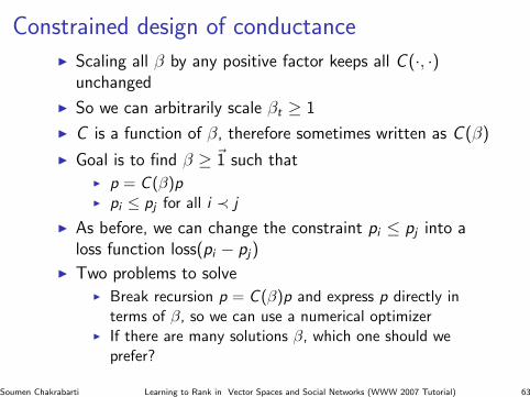
Constrained design of conductanceI Scaling all β by any positive factor keeps all C (·, ·)

unchanged

I So we can arbitrarily scale βt ≥ 1

I C is a function of β, therefore sometimes written as C (β)

I Goal is to find β ≥ ~1 such thatI p = C (β)pI pi ≤ pj for all i ≺ j

I As before, we can change the constraint pi ≤ pj into aloss function loss(pi − pj)

I Two problems to solveI Break recursion p = C (β)p and express p directly in

terms of β, so we can use a numerical optimizerI If there are many solutions β, which one should we

prefer?


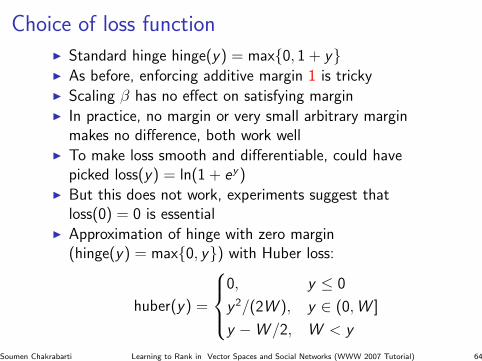
Choice of loss functionI Standard hinge hinge(y) = max0, 1 + yI As before, enforcing additive margin 1 is trickyI Scaling β has no effect on satisfying marginI In practice, no margin or very small arbitrary margin

makes no difference, both work wellI To make loss smooth and differentiable, could have

picked loss(y) = ln(1 + ey)I But this does not work, experiments suggest that

loss(0) = 0 is essentialI Approximation of hinge with zero margin

(hinge(y) = max0, y) with Huber loss:

huber(y) =

0, y ≤ 0

y 2/(2W ), y ∈ (0, W ]

y −W /2, W < y


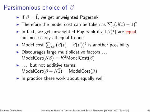
Parsimonious choice of βI If β = ~1, we get unweighted Pagerank

I Therefore the model cost can be taken as∑

t(β(t)− 1)2

I In fact, we get unweighted Pagerank if all β(t) are equal,not necessarily all equal to one

I Model cost∑

t,t′(β(t)− β(t ′))2 is another possibility

I Discourages large multiplicative factors . . .ModelCost(Kβ) = K 2ModelCost(β)

I . . . but not additive terms:ModelCost(β + K~1) = ModelCost(β)

I In practice these work about equally well


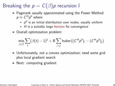
Breaking the p = C (β)p recursion II Pagerank usually approximated using the Power Method

p ≈ CHp0 whereI p0 is an initial distribution over nodes, usually uniformI H is a suitably large horizon for convergence

I Overall optimization problem:

minβ≥~1

∑t

(β(t)− 1)2 + B∑i≺j

huber((CHp0)i − (CHp0)j

)I Unfortunately, not a convex optimization; need some grid

plus local gradient search

I Next: computing gradient


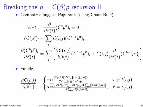
Breaking the p = C (β)p recursion III Compute alongsize Pagerank (using Chain Rule):

∀i∀t :∂

∂β(t)(C 0p0)i = 0

(C hp0)i =∑

j

C (i , j)(C h−1p0)j

∂(C hp0)i

∂β(t)=∑

j

[∂C (i , j)

∂β(t)(C h−1p0)j + C (i , j)

∂

∂β(t)(C h−1p0)j

]I Finally,

∂C (i , j)

∂β(τ)=

−α

β(t(i ,j))P

w [[τ=t(i ,w)]]

(P

w β(t(i ,w)))2τ 6= t(i , j)

αP

w β(t(i ,w))−β(t(i ,j))P

w [[τ=t(i ,w)]]

(P

w β(t(i ,w)))2, τ = t(i , j)


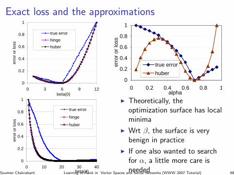
Exact loss and the approximations

0

0.2

0.4

0.6

0.8

1

0 3 6 9 12beta(0)

erro

r or

loss

true error

hinge

huber

0

0.2

0.4

0.6

0.8

1

0 10 20 30 40beta(4)

erro

r or

loss

true error

hinge

huber

0

0.2

0.4

0.6

0.8

1

0 0.2 0.4 0.6 0.8 1alpha

erro

r or

loss

true error

huber

I Theoretically, theoptimization surface has localminima

I Wrt β, the surface is verybenign in practice

I If one also wanted to searchfor α, a little more care isneededSoumen Chakrabarti Learning to Rank in Vector Spaces and Social Networks (WWW 2007 Tutorial) 68

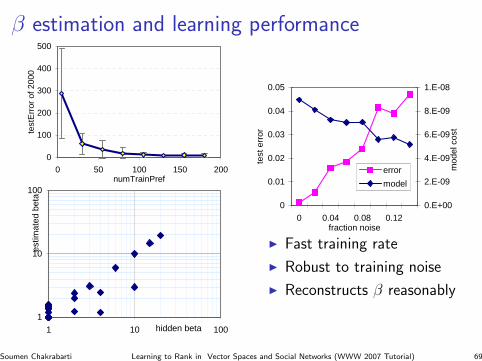
β estimation and learning performance

0

100

200

300

400

500

0 50 100 150 200numTrainPref

test

Err

or o

f 200

0

1

10

100

1 10 100hidden beta

estim

ated

bet

a

0

0.01

0.02

0.03

0.04

0.05

0 0.04 0.08 0.12fraction noise

test

err

or

0.E+00

2.E-09

4.E-09

6.E-09

8.E-09

1.E-08

mod

el c

ost

error

model

I Fast training rate

I Robust to training noise

I Reconstructs β reasonably


Preliminaries









Some sample resultsI Pagerank is score-stable but not rank-stable

I (HITS is not score-stable and not rank-stable)

I More notions of stability, connections with generalization

I Max-margin vector-space ranking is stable

I Ranking based on Laplace smoothing is stable

I Ranking based on constrained circulation is stable


Pagerank is score-stable when G is perturbedI V kept fixed

I Nodes in P ⊂ V get incident links changed in any way(additions and deletions)

I Thus G perturbed to G

I Let the random surfer visit (random) node sequenceX0, X1, . . . in G , and Y0, Y1, . . . in G

I Coupling argument: instead of two random walks, we willdesign one joint walk on (Xi , Yi) such that the marginalsapply to G and G


Coupled random walks on G and GI Pick X0 = Y0 ∼ Multi(r)

I At any step t, with probability 1− α, reset both chains toa common node using teleport r : Xt = Yt ∈r V

I With the remaining probability of α

I If xt−1 = yt−1 = u, say, and u remained unperturbedfrom G to G , then pick one out-neighbor v of uuniformly at random from all out-neighbors of u, and setXt = Yt = v .

I Otherwise, i.e., if xt−1 6= yt−1 or xt−1 was perturbedfrom G to G , pick out-neighbors Xt and Yt

independently for the two walks.


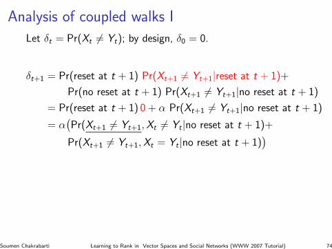
Analysis of coupled walks I

Let δt = Pr(Xt 6= Yt); by design, δ0 = 0.

δt+1 = Pr(reset at t + 1) Pr(Xt+1 6= Yt+1|reset at t + 1)+

Pr(no reset at t + 1) Pr(Xt+1 6= Yt+1|no reset at t + 1)

= Pr(reset at t + 1) 0 + α Pr(Xt+1 6= Yt+1|no reset at t + 1)

= α(Pr(Xt+1 6= Yt+1, Xt 6= Yt |no reset at t + 1)+

Pr(Xt+1 6= Yt+1, Xt = Yt |no reset at t + 1))


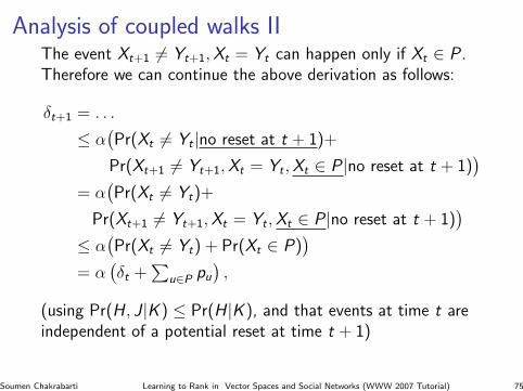
Analysis of coupled walks IIThe event Xt+1 6= Yt+1, Xt = Yt can happen only if Xt ∈ P .Therefore we can continue the above derivation as follows:

δt+1 = . . .

≤ α(Pr(Xt 6= Yt |no reset at t + 1)+

Pr(Xt+1 6= Yt+1, Xt = Yt , Xt ∈ P|no reset at t + 1))

= α(Pr(Xt 6= Yt)+

Pr(Xt+1 6= Yt+1, Xt = Yt , Xt ∈ P|no reset at t + 1))

≤ α(Pr(Xt 6= Yt) + Pr(Xt ∈ P)

)= α

(δt +

∑u∈P pu

),

(using Pr(H , J |K ) ≤ Pr(H |K ), and that events at time t areindependent of a potential reset at time t + 1)


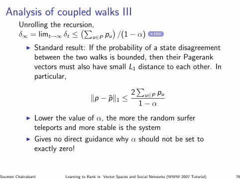
Analysis of coupled walks IIIUnrolling the recursion,δ∞ = limt→∞ δt ≤

(∑u∈P pu

)/(1− α) HW

I Standard result: If the probability of a state disagreementbetween the two walks is bounded, then their Pagerankvectors must also have small L1 distance to each other. Inparticular,

‖p − p‖1 ≤2∑

u∈P pu

1− α

I Lower the value of α, the more the random surferteleports and more stable is the system

I Gives no direct guidance why α should not be set toexactly zero!


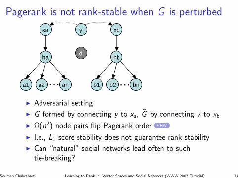
Pagerank is not rank-stable when G is perturbed

xa y xb

ha hb

a1 ana2 b1 bnb2

d

… …

I Adversarial setting

I G formed by connecting y to xa, G by connecting y to xb

I Ω(n2) node pairs flip Pagerank order HW

I I.e., L1 score stability does not guarantee rank stability

I Can “natural” social networks lead often to suchtie-breaking?


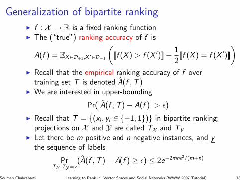
Generalization of bipartite rankingI f : X → R is a fixed ranking functionI The (“true”) ranking accuracy of f is

A(f ) = EX∈D+1,X ′∈D−1

([[f (X ) > f (X ′)]] +

1

2[[f (X ) = f (X ′)]]

)I Recall that the empirical ranking accuracy of f over

training set T is denoted A(f , T )I We are interested in upper-bounding

Pr(|A(f , T )− A(f )| > ε)

I Recall that T = (xi , yi ∈ −1, 1) in bipartite ranking;projections on X and Y are called TX and TY

I Let there be m positive and n negative instances, and ythe sequence of labels

PrTX |TY=y

(A(f , T )− A(f ) ≥ ε) ≤ 2e−2mnε2/(m+n)


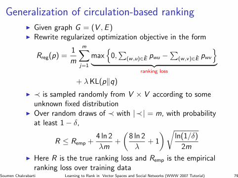
Generalization of circulation-based rankingI Given graph G = (V , E )I Rewrite regularized optimization objective in the form

Rreg(p) =1

m

m∑j=1

max

0,∑

(w ,u)∈E pwu −∑

(w ,v)∈E pwv

︸︷︷︸

ranking loss

+ λ KL(p‖q)

I ≺ is sampled randomly from V × V according to someunknown fixed distribution

I Over random draws of ≺ with |≺| = m, with probabilityat least 1− δ,

R ≤ Remp +4 ln 2

λm+

(8 ln 2

λ+ 1

)√ln(1/δ)

2m

I Here R is the true ranking loss and Remp is the empiricalranking loss over training data


Preliminaries









Preliminaries









Preliminaries









Preliminaries









References I

W. Chu and S. Keerthi, “New approaches to supportvector ordinal regression,” in ICML, 2005, pp. 145–152.http://www.gatsby.ucl.ac.uk/∼chuwei/paper/icmlsvor.pdf

T. Joachims, “Optimizing search engines usingclickthrough data,” in SIGKDD Conference. ACM, 2002.http://www.cs.cornell.edu/People/tj/publications/joachims 02c.pdf

——, “Training linear svms in linear time,” in SIGKDDConference, 2006, pp. 217–226. http://www.cs.cornell.edu/people/tj/publications/joachims 06a.pdf


http://www.gatsby.ucl.ac.uk/~chuwei/paper/icmlsvor.pdf

http://www.gatsby.ucl.ac.uk/~chuwei/paper/icmlsvor.pdf

http://www.cs.cornell.edu/People/tj/publications/joachims_02c.pdf

http://www.cs.cornell.edu/People/tj/publications/joachims_02c.pdf

http://www.cs.cornell.edu/people/tj/publications/joachims_06a.pdf

http://www.cs.cornell.edu/people/tj/publications/joachims_06a.pdf

References II

I. Tsochantaridis, T. Joachims, T. Hofmann, andY. Altun, “Large margin methods for structured andinterdependent output variables,” JMLR, vol. 6, no. Sep,pp. 1453–1484, 2005. http://ttic.uchicago.edu/∼altun/pubs/TsoJoaHofAlt-JMLR.pdf

C. Burges, T. Shaked, E. Renshaw, A. Lazier, M. Deeds,N. Hamilton, and G. Hullender, “Learning to rank usinggradient descent,” in ICML, 2005. http://research.microsoft.com/∼cburges/papers/ICML ranking.pdf

W. W. Cohen, R. E. Shapire, and Y. Singer, “Learning toorder things,” JAIR, vol. 10, pp. 243–270, 1999.http://www.cs.washington.edu/research/jair/volume10/cohen99a.ps


http://ttic.uchicago.edu/~altun/pubs/TsoJoaHofAlt-JMLR.pdf

http://ttic.uchicago.edu/~altun/pubs/TsoJoaHofAlt-JMLR.pdf

http://research.microsoft.com/~cburges/papers/ICML_ranking.pdf

http://research.microsoft.com/~cburges/papers/ICML_ranking.pdf

http://www.cs.washington.edu/research/jair/volume10/cohen99a.ps

http://www.cs.washington.edu/research/jair/volume10/cohen99a.ps

References III

Y. Freund, R. Iyer, R. E. Schapire, and Y. Singer, “Anefficient boosting algorithm for combining preferences,”Journal of Machine Learning Research, vol. 4, pp.933–969, 2003. http://jmlr.csail.mit.edu/papers/volume4/freund03a/freund03a.pdf

S. Agarwal, “Ranking on graph data,” in ICML, 2006, pp.25–32. http://web.mit.edu/shivani/www/Papers/2006/icml06-graph-ranking.pdf

F. Chung, “Laplacians and the Cheeger inequality fordirected graphs,” Annals of Combinatorics, vol. 9, pp.1–19, 2005.http://www.math.ucsd.edu/∼fan/wp/dichee.pdf


http://jmlr.csail.mit.edu/papers/volume4/freund03a/freund03a.pdf

http://jmlr.csail.mit.edu/papers/volume4/freund03a/freund03a.pdf

http://web.mit.edu/shivani/www/Papers/2006/icml06-graph-ranking.pdf

http://web.mit.edu/shivani/www/Papers/2006/icml06-graph-ranking.pdf

http://www.math.ucsd.edu/~fan/wp/dichee.pdf

References IV

J. A. Tomlin, “A new paradigm for ranking pages on theworld wide Web,” in WWW Conference, 2003, pp.350–355. http://www2003.org/cdrom/papers/refereed/p042/paper42 html/p42-tomlin.htm

A. Agarwal, S. Chakrabarti, and S. Aggarwal, “Learning torank networked entities,” in SIGKDD Conference, 2006,pp. 14–23.http://www.cse.iitb.ac.in/∼soumen/doc/netrank

S. Chakrabarti and A. Agarwal, “Learning parameters inentity relationship graphs from ranking preferences,” inPKDD Conference, ser. LNCS, vol. 4213, Berlin, 2006, pp.91–102.http://www.cse.iitb.ac.in/∼soumen/doc/netrank


http://www2003.org/cdrom/papers/refereed/p042/paper42_html/p42-tomlin.htm

http://www2003.org/cdrom/papers/refereed/p042/paper42_html/p42-tomlin.htm

http://www.cse.iitb.ac.in/~soumen/doc/netrank


References V

Z. Nie, Y. Zhang, J.-R. Wen, and W.-Y. Ma, “Object-levelranking: Bringing order to Web objects,” in WWWConference, 2005, pp. 567–574.http://www2005.org/cdrom/docs/p567.pdf

M. Diligenti, M. Gori, and M. Maggini, “Learning Webpage scores by error back-propagation,” in IJCAI, 2005.http://www.ijcai.org/papers/1205.pdf

A. Ng, A. Zheng, and M. Jordan, “Stable algorithms forlink analysis,” in SIGIR Conference. New Orleans: ACM,sep 2001, available fromhttp://www.cs.berkeley.edu/∼ang/.


http://www2005.org/cdrom/docs/p567.pdf

http://www.ijcai.org/papers/1205.pdf

http://www.cs.berkeley.edu/~ang/

References VI

R. Lempel and S. Moran, “Rank-stability andrank-similarity of link-based web ranking algorithms inauthority-connected graphs,” Information Retrieval, vol. 8,no. 2, pp. 245–264, 2005. http://www.cs.technion.ac.il/∼moran/r/PS/stab kluwer.pdf

S. Agarwal and P. Niyogi, “Stability and generalization ofbipartite ranking algorithms,” in COLT, Bertinoro, June2005, pp. 32–47. http://web.mit.edu/shivani/www/Papers/2005/colt05-stability.pdf

A. Agarwal and S. Chakrabarti, “Learning random walksto rank nodes in graphs,” in ICML, 2007.http://www.cse.iitb.ac.in/∼soumen/doc/netrank


http://www.cs.technion.ac.il/~moran/r/PS/stab_kluwer.pdf

http://www.cs.technion.ac.il/~moran/r/PS/stab_kluwer.pdf

http://web.mit.edu/shivani/www/Papers/2005/colt05-stability.pdf

http://web.mit.edu/shivani/www/Papers/2005/colt05-stability.pdf


References VII

D. Zhou and C. J. C. Burges, “Spectral clustering andtransductive learning with multiple views,” in ICML, 2007.http://research.microsoft.com/∼denzho/papers/mv ICML.pdf


http://research.microsoft.com/~denzho/papers/mv_ICML.pdf

http://research.microsoft.com/~denzho/papers/mv_ICML.pdf

Date post:	25-Sep-2018
Category:	Documents
Upload:	nguyentu
View:	214 times
Download:	0 times

Learning to Rank in Vector Spaces and Social Networks …soumen/doc/ · Vector Spaces and Social...

Documents