38
CEE 320 Winter 2006 Signalized Intersections CEE 320 Steve Muench
| Date post: | 23-Jan-2018 |
| Category: |
Engineering |
| Upload: | hossam-shafiq-i |
| View: | 630 times |
| Download: | 4 times |

CE
E 3
20
Win
ter
2006
Signalized Intersections
CEE 320
Steve Muench

CE
E 3
20
Win
ter
2006
Outline
1. Key Definitions
2. Baseline Assumptions
3. Control Delay
4. Signal Analysis a. D/D/1
b. Random Arrivals
c. LOS Calculation
d. Optimization
CE
E 3
20
Win
ter
2006
Key Definitions (1)
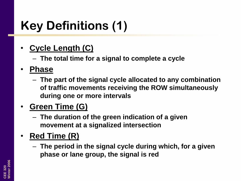
• Cycle Length (C)
– The total time for a signal to complete a cycle
• Phase
– The part of the signal cycle allocated to any combination
of traffic movements receiving the ROW simultaneously
during one or more intervals
• Green Time (G)
– The duration of the green indication of a given
movement at a signalized intersection
• Red Time (R)
– The period in the signal cycle during which, for a given
phase or lane group, the signal is red

CE
E 3
20
Win
ter
2006
Key Definitions (2)
• Change Interval (Y)
– Yellow time
– The period in the signal cycle during which, for a given
phase or lane group, the signal is yellow
• Clearance Interval (AR)
– All red time
– The period in the signal cycle during which all
approaches have a red indication
CE
E 3
20
Win
ter
2006
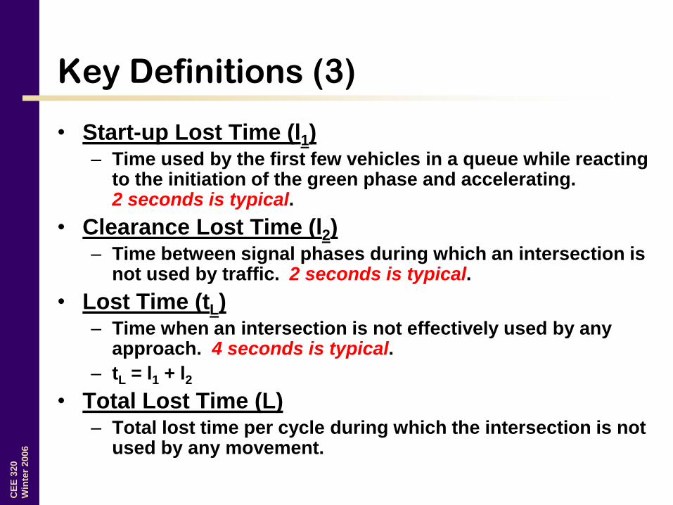
Key Definitions (3)
• Start-up Lost Time (l1) – Time used by the first few vehicles in a queue while reacting
to the initiation of the green phase and accelerating. 2 seconds is typical.
• Clearance Lost Time (l2) – Time between signal phases during which an intersection is
not used by traffic. 2 seconds is typical.
• Lost Time (tL) – Time when an intersection is not effectively used by any
approach. 4 seconds is typical.
– tL = l1 + l2
• Total Lost Time (L) – Total lost time per cycle during which the intersection is not
used by any movement.

CE
E 3
20
Win
ter
2006
Key Definitions (4)
• Effective Green Time (g) – Time actually available for movement
– g = G + Y + AR – tL
• Extension of Effective Green Time (e) – The amount of the change and clearance interval at the
end of a phase that is usable for movement of vehicles
• Effective Red Time (r) – Time during which a movement is effectively not
permitted to move.
– r = R + tL
– r = C – g

CE
E 3
20
Win
ter
2006
Key Definitions (5)
• Saturation Flow Rate (s) – Maximum flow that could pass through an intersection if
100% green time was allocated to that movement.
– s = 3600/h
• Approach Capacity (c) – Saturation flow times the proportion of effective green
– c = s × g/C
• Peak Hour Factor (PHF) – The hourly volume during the maximum-volume hour of
the day divided by the peak 15-minute flow rate within the peak hour; a measure of traffic demand fluctuation within the peak hour.
CE
E 3
20
Win
ter
2006
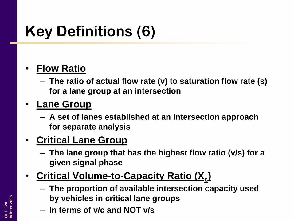
Key Definitions (6)
• Flow Ratio
– The ratio of actual flow rate (v) to saturation flow rate (s)
for a lane group at an intersection
• Lane Group
– A set of lanes established at an intersection approach
for separate analysis
• Critical Lane Group
– The lane group that has the highest flow ratio (v/s) for a
given signal phase
• Critical Volume-to-Capacity Ratio (Xc)
– The proportion of available intersection capacity used
by vehicles in critical lane groups
– In terms of v/c and NOT v/s

fro
m H
igh
wa
y C
ap
acity M
an
ua
l 2
00
0

CE
E 3
20
Win
ter
2006
Baseline Assumptions
• D/D/1 queuing
• Approach arrivals < departure capacity
– (no queue exists at the beginning/end of a
cycle)
CE
E 3
20
Win
ter
2006
Quantifying Control Delay
• Two approaches
– Deterministic (uniform) arrivals (Use D/D/1)
– Probabilistic (random) arrivals (Use empirical equations)
• Total delay can be expressed as
– Total delay in an hour (vehicle-hours, person-hours)
– Average delay per vehicle (seconds per vehicle)

CE
E 3
20
Win
ter
2006
D/D/1 Signal Analysis (Graphical)
Arrival
Rate
Departure
Rate
Time
Ve
hic
les
Maximum delay
Maximum queue
Total vehicle delay per cycle
Red Red Red Green Green Green
Queue dissipation

CE
E 3
20
Win
ter
2006
D/D/1 Signal Analysis – Numerical
• Time to queue dissipation after the start of effective green
• Proportion of the cycle with a queue
• Proportion of vehicles stopped
0.1
10
rt
c
trPq
0
qs P
c
tr
gr
trP
00
c
t
c
t
gr
trPs
000
CE
E 3
20
Win
ter
2006
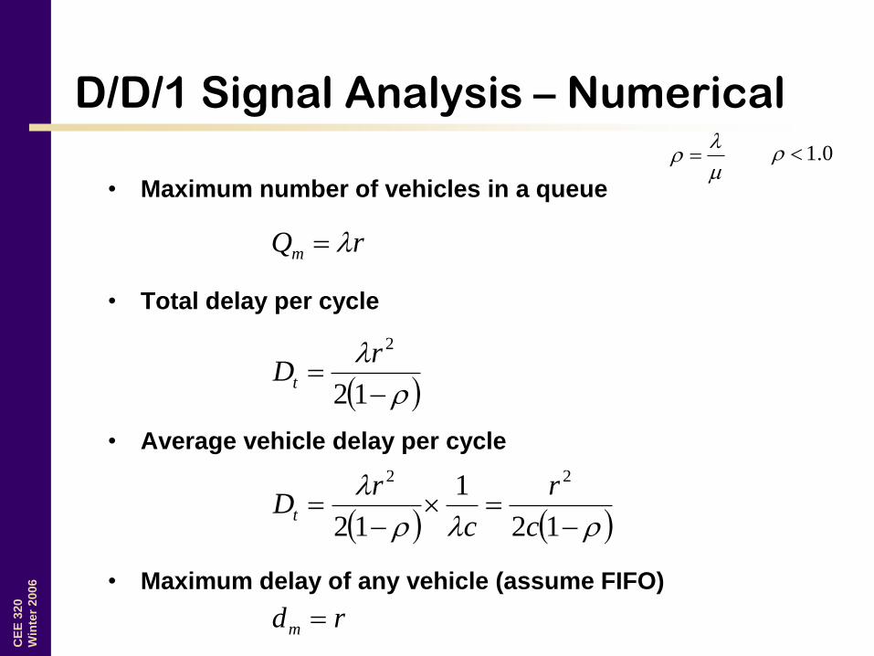
D/D/1 Signal Analysis – Numerical
• Maximum number of vehicles in a queue
• Total delay per cycle
• Average vehicle delay per cycle
• Maximum delay of any vehicle (assume FIFO)
0.1
rQm
12
2rDt
12
1
12
22
c
r
c
rDt
rdm

CE
E 3
20
Win
ter
2006
Signal Analysis – Random Arrivals
• Webster’s Formula (1958) - empirical
d’ = avg. veh. delay assuming random arrivals
d = avg. veh. delay assuming uniform arrivals (D/D/1)
x = ratio of arrivals to departures (c/g)
g = effective green time (sec)
c = cycle length (sec)
)/(52
3/1
2
2
65.012
' cgxc
x
xdd
CE
E 3
20
Win
ter
2006
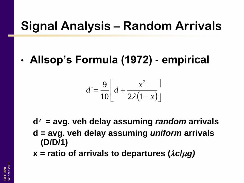
Signal Analysis – Random Arrivals
• Allsop’s Formula (1972) - empirical
d’ = avg. veh delay assuming random arrivals
d = avg. veh delay assuming uniform arrivals (D/D/1)
x = ratio of arrivals to departures (c/g)
x
xdd
1210
9'
2

CE
E 3
20
Win
ter
2006
Definition – Level of Service (LOS)
• Chief measure of “quality of service”
– Describes operational conditions within a traffic
stream
– Does not include safety
– Different measures for different facilities
• Six levels of service (A through F)
CE
E 3
20
Win
ter
2006
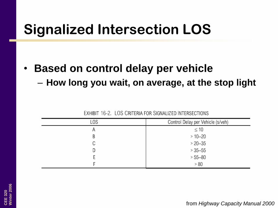
Signalized Intersection LOS
• Based on control delay per vehicle
– How long you wait, on average, at the stop light
from Highway Capacity Manual 2000

CE
E 3
20
Win
ter
2006
Typical Approach
• Split control delay into three parts – Part 1: Delay calculated assuming uniform arrivals (d1).
This is essentially a D/D/1 analysis.
– Part 2: Delay due to random arrivals (d2)
– Part 3: Delay due to initial queue at start of analysis time
period (d3). Often assumed zero.
321 ddPFdd
d = Average signal delay per vehicle in s/veh
PF = progression adjustment factor
d1, d2, d3 = as defined above

CE
E 3
20
Win
ter
2006
Uniform Delay (d1)
C
gX
C
gC
d
,1min1
15.0
1
d1 = delay due to uniform arrivals (s/veh)
C = cycle length (seconds)
g = effective green time for lane group (seconds)
X = v/c ratio for lane group

CE
E 3
20
Win
ter
2006
Incremental Delay (d2)
cT
kIXXXTd
811900
2
2
d2 = delay due to random arrivals (s/veh)
T = duration of analysis period (hours). If the analysis is based on the
peak 15-min. flow then T = 0.25 hrs.
k = delay adjustment factor that is dependent on signal controller mode.
For pretimed intersections k = 0.5. For more efficient intersections k
< 0.5.
I = upstream filtering/metering adjustment factor. Adjusts for the effect of
an upstream signal on the randomness of the arrival pattern. I = 1.0
for completely random. I < 1.0 for reduced variance.
c = lane group capacity (veh/hr)
X = v/c ratio for lane group
CE
E 3
20
Win
ter
2006
Initial Queue Delay (d3)
• Applied in cases where X > 1.0 for the
analysis period
– Vehicles arriving during the analysis period
will experience an additional delay because
there is already an existing queue
• When no initial queue…
– d3 = 0

CE
E 3
20
Win
ter
2006
Control Optimization
• Conflicting Operational Objectives
– minimize vehicle delay
– minimize vehicle stops
– minimize lost time
– major vs. minor service (progression)
– pedestrian service
– reduce accidents/severity
– reduce fuel consumption
– Air pollution

CE
E 3
20
Win
ter
2006
The “Art” of Signal Optimization
• Long Cycle Length – High capacity (reduced lost time)
– High delay on movements that are not served
– Pedestrian movements? Number of Phases?
• Short Cycle Length – Reduced capacity (increased lost time)
– Reduced delay for any given movement

CE
E 3
20
Win
ter
2006
Minimum Cycle Length
n
i ci
c
c
s
vX
XLC
1
min
Cmin = estimated minimum cycle length (seconds)
L = total lost time per cycle (seconds), 4 seconds per
phase is typical
(v/s)ci = flow ratio for critical lane group, i (seconds)
Xc = critical v/c ratio for the intersection
CE
E 3
20
Win
ter
2006
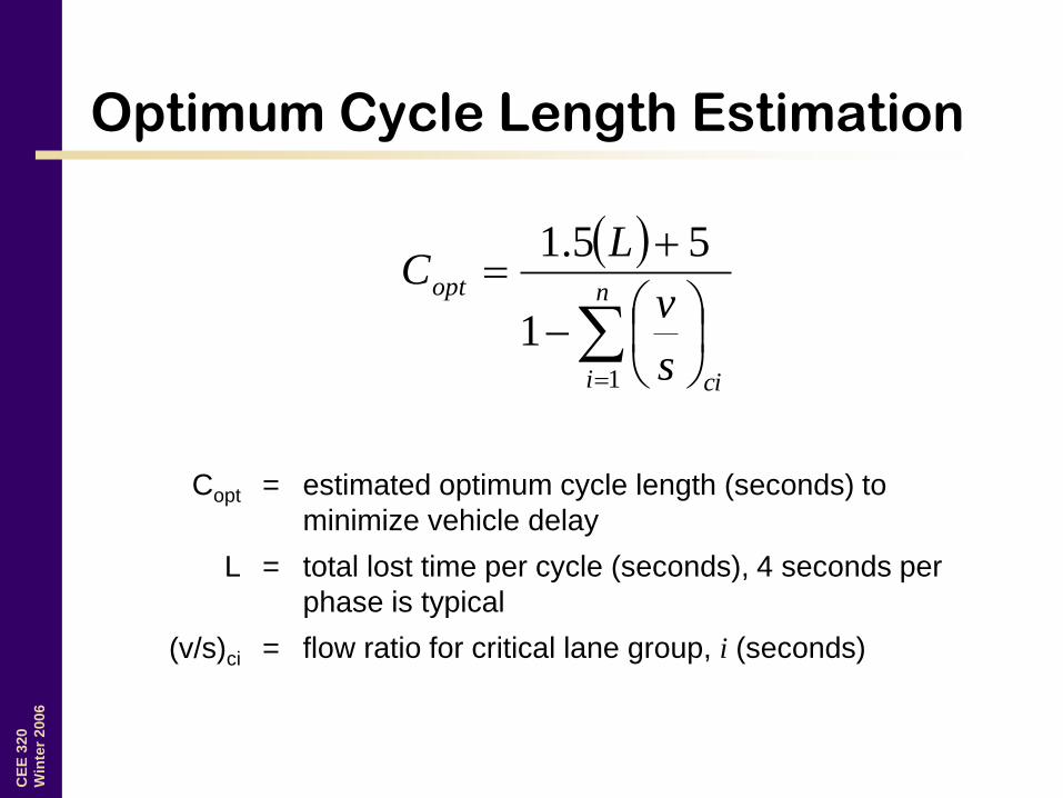
Optimum Cycle Length Estimation
n
i ci
opt
s
v
LC
1
1
55.1
Copt = estimated optimum cycle length (seconds) to
minimize vehicle delay
L = total lost time per cycle (seconds), 4 seconds per
phase is typical
(v/s)ci = flow ratio for critical lane group, i (seconds)
CE
E 3
20
Win
ter
2006
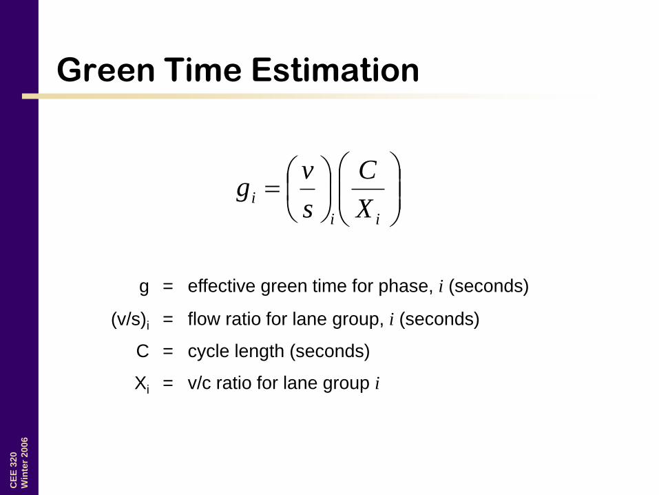
Green Time Estimation
ii
iX
C
s
vg
g = effective green time for phase, i (seconds)
(v/s)i = flow ratio for lane group, i (seconds)
C = cycle length (seconds)
Xi = v/c ratio for lane group i
CE
E 3
20
Win
ter
2006
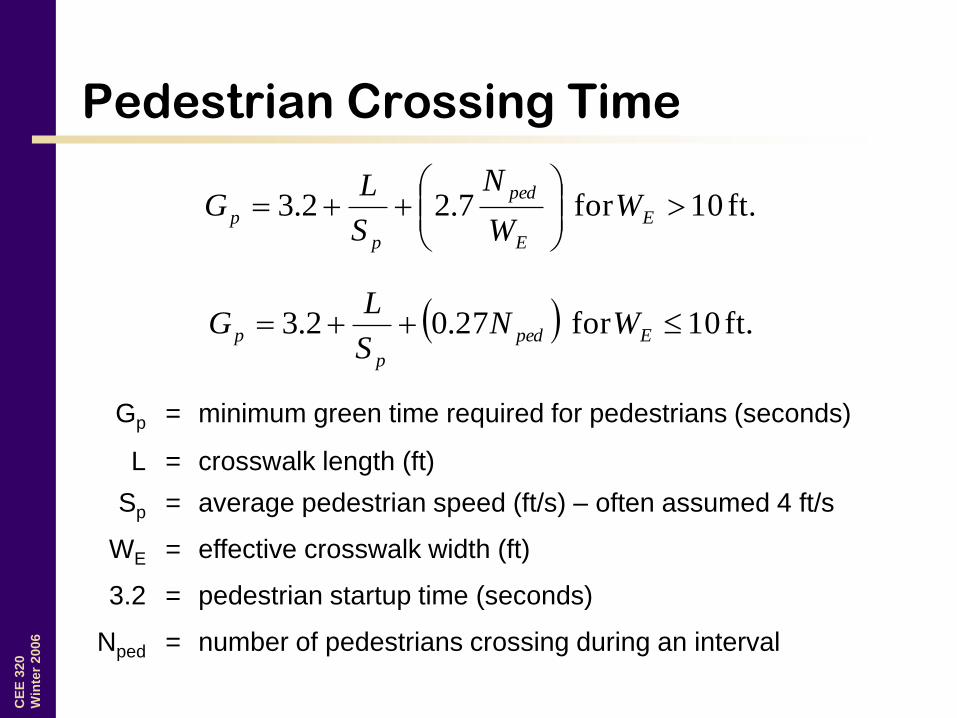
Pedestrian Crossing Time
ft. 10for 7.22.3
E
E
ped
p
p WW
N
S
LG
ft. 10for 27.02.3 Eped
p
p WNS
LG
Gp = minimum green time required for pedestrians (seconds)
L = crosswalk length (ft)
Sp = average pedestrian speed (ft/s) – often assumed 4 ft/s
WE = effective crosswalk width (ft)
3.2 = pedestrian startup time (seconds)
Nped = number of pedestrians crossing during an interval

CE
E 3
20
Win
ter
2006
Effective Width (WE)
from Highway Capacity Manual 2000

CE
E 3
20
Win
ter
2006
Example
An intersection operates using a
simple 3-phase design as
pictured.
NB
SB
EB
WB
Phase Lane
group
Saturation Flows
1 SB 3400 veh/hr
2 NB 3400 veh/hr
3 EB 1400 veh/hr
WB 1400 veh/hr

CE
E 3
20
Win
ter
2006
Example
SB
NB
EB
WB
30
150
50
30
400
100
1000
200
300 20
What is the sum of the flow ratios for the critical lane groups?
What is the total lost time for a signal cycle assuming 2 seconds of
clearance lost time and 2 seconds of startup lost time per phase?

CE
E 3
20
Win
ter
2006
Example
Calculate an optimal signal timing (rounded up to the nearest 5
seconds) using Webster’s formula.
n
i
ci
opt
sv
LC
1
1
55.1
CE
E 3
20
Win
ter
2006
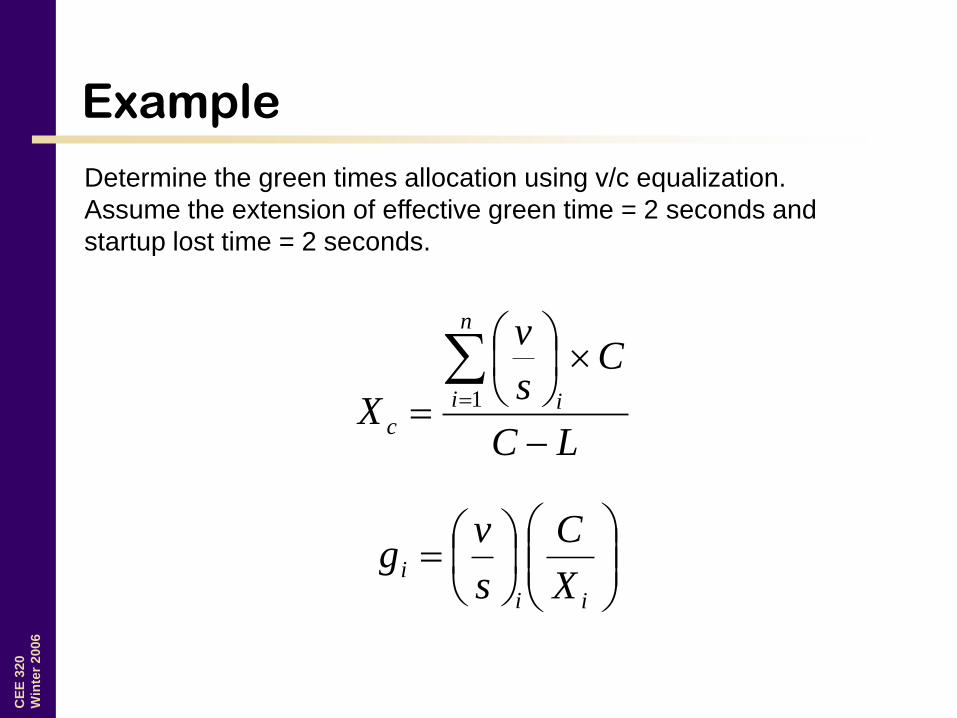
Example
Determine the green times allocation using v/c equalization.
Assume the extension of effective green time = 2 seconds and
startup lost time = 2 seconds.
ii
iX
C
s
vg
LC
Cs
v
X
n
i ic
1
CE
E 3
20
Win
ter
2006
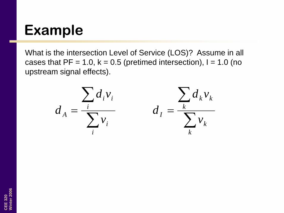
Example
What is the intersection Level of Service (LOS)? Assume in all
cases that PF = 1.0, k = 0.5 (pretimed intersection), I = 1.0 (no
upstream signal effects).
i
i
i
ii
Av
vd
d
k
k
k
kk
Iv
vd
d

CE
E 3
20
Win
ter
2006
Example
Is this signal adequate for pedestrians? A pedestrian count showed
5 pedestrians crossing the EB and WB lanes on each side of the
intersection and 10 pedestrians crossing the NB and SB
crosswalks on each side of the intersection. Lanes are 12 ft. wide.
The effective crosswalk widths are all 10 ft.
ft 10for 27.02.3 Eped
p
p WNS
LG

CE
E 3
20
Win
ter
2006
Signal Installation: “Warrants”
• Manual of Uniform Traffic Control Devices (MUTCD)
• Apply these rules to determine if a signal is “warranted” at an intersection
• If warrants are met, doesn’t mean signals or control is mandatory
• 8 major warrants
• Multiple warrants usually required for recommending control
http://mutcd.fhwa.dot.gov/
FYI – NOT TESTABLE
CE
E 3
20
Win
ter
2006
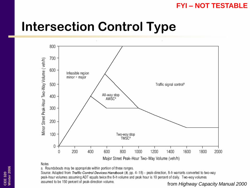
Intersection Control Type
from Highway Capacity Manual 2000
FYI – NOT TESTABLE

CE
E 3
20
Win
ter
2006
Primary References
• Mannering, F.L.; Kilareski, W.P. and Washburn, S.S. (2003).
Principles of Highway Engineering and Traffic Analysis, Third Edition
(Draft). Chapter 7
• Transportation Research Board. (2000). Highway Capacity Manual.
National Research Council, Washington, D.C.


