Lecture 6 -...

Lecture 6

FRTN10 Multivariable Control

Automatic Control LTH, 2018

Course Outline

L1–L5 Specifications, models and loop-shaping by hand

L6–L8 Limitations on achievable performance

6 Controllability/observability, multivariable

poles/zeros

7 Fundamental limitations

8 Decentralized control

L9–L11 Controller optimization: analytic approach

L12–L14 Controller optimization: numerical approach

L15 Course review

Automatic Control LTH, 2018 Lecture 6 FRTN10 Multivariable Control

Lecture 6 – Outline

1 Controllability and observability, Gramians

2 Multivariable poles and zeros

3 Minimal realizations


Example: Ball in the Hoop

input ω

output θ

Üθ + c Ûθ + kθ = Ûω

Can you reach θ = π/4, Ûθ = 0? Can you stay there?


Example: Two water tanks

u1u1

u2 u2x1

x1

x2

ax2 a ≥ 1

Ûx1 = −x1 + u1 y1 = x1 + u2

Ûx2 = −ax2 + u1 y2 = ax2 + u2

Can you reach y1 = 1, y2 = 2? Can you stay there?



1 Controllability and observability




Review: State feedback and controllability

Process

{Ûx = Ax + Bu

y = Cx

State-feedback control

u = − Lx + lrr

Closed-loop system

{Ûx = (A − BL)x + Blrr

y = Cx

rlr +

uÛx = Ax + Bu

y = Cx

x

−L

If the system (A, B) is controllable then we can place the eigenvalues of

(A − BL) arbitrarilyAutomatic Control LTH, 2018 Lecture 6 FRTN10 Multivariable Control

Review: State observers and observability

Process

{Ûx = Ax + Bu

y = Cx

Observer (“Kalman filter”)

Û̂x = Ax̂ + Bu + K(y − Cx̂)

Estimation/observer error x̃ = x − x̂:

Û̃x = (A − KC)x̃

If the system (A,C) is observable then we can place the eigenvalues

of (A − KC) arbitrarily


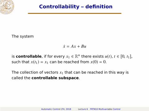
Controllability – definition

The system

Ûx = Ax + Bu

is controllable, if for every x1 ∈ Rn there exists u(t), t ∈ [0, t1],

such that x(t1) = x1 can be reached from x(0) = 0.

The collection of vectors x1 that can be reached in this way is

called the controllable subspace.


Controllability criteria

The following controllability criteria for a system Ûx = Ax + Bu of

order n are equivalent:

(i) rank [B AB . . . An−1B] = n

(ii) rank [λI − A B] = n for all λ ∈ C

If the system is stable, define the controllability Gramian

Wc =

∫ ∞

0

eAtBBT eAT tdt

For such systems there is a third equivalent criterion:

(iii) The controllability Gramian is non-singular


Interpretation of the controllability Gramian

The inverse of the controllability Gramian measures how difficult

it is to reach different states.

In fact, the minimum control energy required to reach x = x1

starting from x = 0 satisfies

∫ ∞

0

|u(t)|2dt = xT1

W−1

c x1

(For proof, see the lecture notes.)


Computing the controllability Gramian

The controllability Gramian Wc =

∫ ∞

0eAtBBT eAT tdt can be

computed by solving the Lyapunov equation

AWc +WcAT+ BBT

= 0

(For proof, see the lecture notes.)

(Matlab: Wc = lyap(A,B*B’))

Q: Where have we seen this equation before?



u1u1

u2 u2x1

x1

x2

ax2

Ûx1 = −x1 + u1 Ûx2 = −ax2 + u1

Controllability Gramian: Wc =

∫ ∞

0

[e−t

e−at

] [e−t

e−at

]Tdt =

[1

2

1

a+11

a+1

1

2a

]

Wc close to singular when a ≈ 1. Interpretation?


Example cont’d

Matlab:

>> a = 1.25; A = [-1 0; 0 -1*a]; B = [1; 1];

>> CM = [B A*B], rank(CM)

CM =

1.0000 -1.0000

1.0000 -1.2500

ans =

2

>> Wc = lyap(A,B*B')

Wc =

0.5000 0.4444

0.4444 0.4000

>> invWc = inv(Wc)

invWc =

162.0 -180.0

-180.0 202.5

−0.6 −0.4 −0.2 0 0.2 0.4 0.6 0.8−0.8

−0.6

−0.4

−0.2

0

0.2

0.4

0.6

x1

x2

[x1 x

2] * inv(S) * [x

1 ; x

2] =1

Plot of[x1 x2

]· W−1

c

[x1

x2

]= 1

corresponds to the states we can reach by∫ ∞

0|u(t)|2dt = 1.


Observability – definition

The system

Ûx(t) = Ax(t)

y(t) = Cx(t)

is observable, if the initial state x(0) = x0 ∈ Rn can be uniquely

determined by the output y(t), t ∈ [0, t1].

The collection of vectors x0 that cannot be distinguished from

x = 0 is called the unobservable subspace.


Observability criteria

The following observability criteria for a system Ûx(t) = Ax(t),

y(t) = Cx(t) of order n are equivalent:

(i) rank

C

CA...

CAn−1

= n

(ii) rank

[λI − A

C

]= n for all λ ∈ C

If the system is stable, define the observability Gramian

Wo =

∫ ∞

0

eAT tCTCeAtdt

For such systems there is a third equivalent statement:

(iii) The observability Gramian is non-singular


Interpretation of the observability Gramian

The observability Gramian measures how easy it is to distinguish

an initial state from zero by observing the output.

In fact, the influence of the initial state x(0) = x0 on the output

y(t) satisfies

∫ ∞

0

|y(t)|2dt = xT0

Wox0


Computing the observability Gramian

The observability Gramian Wo =

∫ ∞

0eAT tCTCeAtdt can be

computed by solving the Lyapunov equation

ATWo +WoA + CTC = 0

(Matlab: Wo = lyap(A’,C’*C))


Mini-problem

Is the water tank system with a = 1 observable?

What if only y1 is available?







Poles and zeros

Ûx = Ax + Bu

y = Cx + Du

Y (s) = [C(sI − A)−1B + D]︸︷︷︸

G(s)

U(s)

For scalar systems,

the points p ∈ C where G(p) = ∞ are called poles

the points z ∈ C where G(z) = 0 are called zeros


Poles and zeros

For multivariable systems,

the points p ∈ C where any Gi j(p) = ∞ are called poles

the points z ∈ C where G(z) loses rank are called

(transmission) zeros

Example:

G(s) =

2

s+1

3

s+2

1

s+1

1

s+1

Poles: −2 and −1 (but what about their multiplicity?)

Zeros: 1 (but how to find them?)


Poles and zeros

For multivariable systems,

the points p ∈ C where any Gi j(p) = ∞ are called poles

the points z ∈ C where G(z) loses rank are called

(transmission) zeros

Example:

G(s) =

2

s+1

3

s+2

1

s+1

1

s+1

Poles: −2 and −1 (but what about their multiplicity?)

Zeros: 1 (but how to find them?)


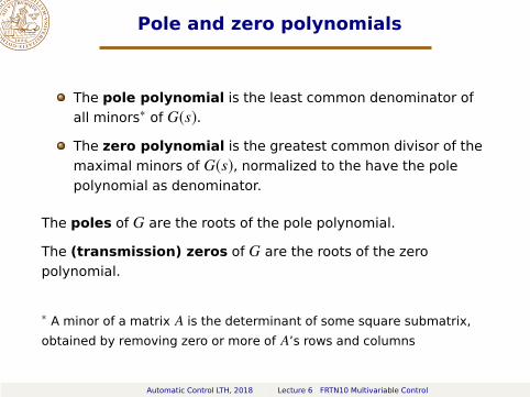
Pole and zero polynomials

The pole polynomial is the least common denominator of

all minors∗ of G(s).

The zero polynomial is the greatest common divisor of the

maximal minors of G(s), normalized to the have the pole

polynomial as denominator.

The poles of G are the roots of the pole polynomial.

The (transmission) zeros of G are the roots of the zero

polynomial.

∗ A minor of a matrix A is the determinant of some square submatrix,

obtained by removing zero or more of A’s rows and columns


Poles and zeros – example

G(s) =

2

s+1

3

s+2

1

s+1

1

s+1

Poles: Minors: 2

s+1, 3

s+2, 1

s+1, 1

s+1, 2

(s+1)2− 3

(s+1)(s+2)=

−(s−1)

(s+1)2(s+2)

The least common denominator is (s + 1)2(s + 2), giving the poles

−2 (with multiplicity 1) and −1 (with multiplicity 2)

Zeros: Maximal minor:−(s−1)

(s+1)2(s+2)(already normalized)

The greatest common divisor is s − 1, giving the (transmission)

zero 1 (with multiplicity 1)

(Matlab: tzero(G))



G(s) =

2

s+1

3

s+2

1

s+1

1

s+1

Poles: Minors: 2

s+1, 3

s+2, 1

s+1, 1

s+1, 2

(s+1)2− 3

(s+1)(s+2)=

−(s−1)

(s+1)2(s+2)







(Matlab: tzero(G))



G(s) =

2

s+1

3

s+2

1

s+1

1

s+1

Poles: Minors: 2

s+1, 3

s+2, 1

s+1, 1

s+1, 2

(s+1)2− 3

(s+1)(s+2)=

−(s−1)

(s+1)2(s+2)







(Matlab: tzero(G))


Interpretation of poles and zeros

Poles:

A pole p is associated with the state response x(t) = x0ept

A pole p is an eigenvalue of A

Zeros:

A zero z means that an input u(t) = u0ezt is blocked

For a multivariable system, blocking occurs only in a certain

input direction

A zero describes how inputs and outputs couple to states

0 2 4 6 8 10 12 14 16 18 20−1

−0.8

−0.6

−0.4

−0.2

0

0.2

0.4

0.6

0.8

1

u y

0 2 4 6 8 10 12 14 16 18 20−0.05

0

0.05

0.1

0.15

0.2

0.25

0.3

0.35

0.4


Example: Ball in the Hoop

input ω

output θ

Üθ + c Ûθ + kθ = Ûω

The transfer function from ω to θ is ss2+cs+k

. The zero in s = 0

makes it impossible to control the stationary position of the ball.

Zeros are not affected by feedback!



u1u1

u2 u2x1

x1

x2

2x2

Ûx1 = −x1 + u1 y1 = x1 + u2

Ûx2 = −2x2 + u1 y2 = 2x2 + u2

G(s) =

[1

s+11

2

s+21

]det G(s) =

−s

(s + 1)(s + 2)

The system has a zero in the origin! At stationarity y1 = y2.


Plot singular values of G(iω) vs frequency

» s=tf(’s’)

» G=[1/(s+1) 1 ; 2/(s+2) 1]

» sigma(G) ; plot singular values

% Alt. for a certain frequency:

» w=1;

» A = freqresp(G,i*w);

» [U,S,V] = svd(A)10

−210

−110

010

110

210

−3

10−2

10−1

100

101

Singular Values

Frequency (rad/sec)

Sin

gu

lar

Va

lue

s (

ab

s)

The largest singular value of G(iω) =

[1

iω+11

2

iω+21

]is fairly constant.

This is due to the second input. The first input makes it possible

to control the difference between the two tanks, but mainly near

ω = 1 where the dynamics make a difference.







Minimal realization – definition

Given G(s), any state-space model (A, B,C,D) that is both

controllable and observable and has the same input–output

behavior as G(s) is called aminimal realization.

A transfer function with n poles (counting multiplicity) has a

minimal realization of order n.


Realization in diagonal form

Consider a transfer function with partial fraction expansion

G(s) =

n∑

i=1

CiBi

s − pi+ D

This has the realization

Ûx(t) =

p1I 0

. . .

0 pnI

x(t) +

B1

...

Bn

u(t)

y(t) =[C1 . . . Cn

]x(t) + Du(t)

The rank of the matrix CiBi determines the necessary number of

columns in Bi and the multiplicity of the pole pi.


Realization of multivariable system – example 1

To find a minimal realization for the system

G(s) =

2

s+1

3

s+2

1

s+1

1

s+1

with poles in −2 and −1 (double), write the transfer matrix as

(e.g.)

G(s) =

[2

1

] [1 0

]

s + 1+

[0

1

] [0 1

]

s + 1+

[3

0

] [0 1

]

s + 2

giving the realization

Ûx =

−1 0 0

0 −1 0

0 0 −2

x +

1 0

0 1

0 1

u

y =

2 0 3

1 1 0

x


Realization of multivariable system – example 2

To find state space-realization for the system

G(s) =

[1

s+1

2

(s+1)(s+3)6

(s+2)(s+4)1

s+2

]

write the transfer matrix as

[1

s+1

1

s+1− 1

s+33

s+2− 3

s+4

1

s+2

]=

[1

0

] [1 1

]

s + 1+

[0

1

] [3 1

]

s + 2+

[1

0

] [0 −1

]

s + 3+

[0

1

] [−3 0

]

s + 4

This gives the realization

Ûx1(t)

Ûx2(t)

Ûx3(t)

Ûx4(t)

=

−1 0 0 0

0 −2 0 0

0 0 −3 0

0 0 0 −4

x1(t)

x2(t)

x3(t)

x4(t)

+

1 1

3 1

0 −1

−3 0

[u1(t)

u2(t)

]

[y1(t)

y2(t)

]=

[1 0 1 0

0 1 0 1

]x(t)


Summary

Gramians give quantitative answers to how controllable or

observable a system is in different state directions

Warning: They do not reveal some important

frequency-domain information (see next lecture)

A multivariable zero blocks input signals a certain direction

A minimal state-space realization describes the controllable

and observable subspace of a system


Date post:	30-May-2020
Category:	Documents
Upload:	others
View:	3 times
Download:	0 times

Lecture 6 -...

Documents