6-1

Lecture Note #6(Chap.10)

CBE 702Korea University

Prof. Dae Ryook Yang

System Modeling and Identification

6-2

Chap.10 Model Approximation

• Model approximation– Simplification, approximation and order reduction of models

• Model reduction– Model order reduction in a linear system

• Balanced realization• Pade approximation• Moment matching• Continued fraction approximation

– Model approximation of a nonlinear system by a linear one• Linearization• Describing function analysis

– Approximation of the nonlinear system by ignoring higher-orderharmonics

6-3

• Linearization– Nonlinear differential equation:– Linearization:

• Discretization– Sampling time: h

where

• Some heuristic model reduction methods (For linear system only)

– Polynomial truncation

– Method of dominating poles

– Pole-zero cancellations

( , )x f x u=&0 0 0 0 0 0 0( , )( ) ( , )( )x ux f f x u x x f x u u u≈ + − + −&

1( ) ( ) ( )

( ) ( )k k k

k k

x x ux t Fx t Gu t

y Cxy t Cx t

Φ Γ+ = += + ⇒ ==

&

0and

hFh Fse e GdsΦ Γ= = ∫

1 1 2 1 1 1( ) 0.22 /(1 0.7 0.08 ) 0.22 /(1 0.8 )(1 0.1 )H z z z z z z z− − − − − −= − − = − +

1 11( ) 0.3 /(1 0.7 )H z z z− −= −

1 12( ) 0.2 /(1 0.8 )H z z z− −= −

1 13( ) 1.1 /(1 0.1 )H z z z− −= + Cancel (1−0.8z-1) with (1−0.78z-1)

6-4

Balanced Realization andModel Reduction

• The Reachability Gramian

– What states can be reached with a given input energy assuming that x0=0?– Given finite input energy:– States:

– Input Sequence for desired xN:

1: k k k nk

k k

x x uS x R

y CxΦ Γ+ = +

∈ =

1( ) N T

uu k kkJ u e u u E

== = ≤∑

1 21 0 N-11

[ ][ u ]N N k N N TN k N Nk

x u u UΦ Γ Φ Φ Γ ψ− − −−=

= = =∑ L L1( )T T

N N N N NU xψ ψ ψ−=1

1( ) N T T T

k k N N N N NkJ u u u U U x P x E−

== = = ≤∑

1

0where ( ) 0NT k T T k

N N N kP ψ ψ Φ ΓΓ Φ−

== = ≥∑

Bound on the reachable states at time N

PN : Reachability Gramian

1 0T T T TN NP P P PΦ Φ ΓΓ Φ Φ ΓΓ+ = + ⇒ − + = Lyapunov equation

6-5

• The Observability Gramian– What states energy is necessary for all uk=0 in order to obtain a specified

output energy?– Specified output energy:

– Reachability Gramian decides the minimum input energy to drive a systemfrom x0 to xN.

– Observability Gramian decides the maximum output energy that the initialstate x0 can generate.

0( ) T

yy k kkJ y e y y E∞

== = =∑

10 00

( ) T Tk kk

J y y y x Q x E∞ −=

= = =∑1 0 ( 0, )k

k k k ky Cx C x C x u kΦ Φ−= = = = = ∀L ∵

0where ( ) 0T k T k

kQ C CΦ Φ∞

== ≥∑ Q : Observability Gramian

0T T T TQ Q C C Q Q C CΦ Φ Φ Φ= + ⇒ − + = Lyapunov equation

1 10

( ( ) )T T T k T k Tk

Q C C C C CCΦ Φ Φ Φ Φ∞ + +=

+ = + =∑

6-6

• Balanced Realization– Reachability and observability Gramians P and Q define matrices that

describe the sensitivity of the input-output map in different directions ofstate space.

– Consider a state-space transformation zk=Txk, then the system becomes

– Different state-space realization may result in different Gramians– Balanced realization: Pz=Qz

– Algorithm using Cholesky factorization

– If some σi’s are relatively small, the Σ can be reduced and the resultingtransformation produces a balanced model resuction.

11

1: k k k

k k

z T T z T uS

y CT z

Φ Γ−+

−

= +

=1

Tz

Tz

P TPTQ T QT− −

=⇒

=

1 2( , ) (where ( ))z z i iP Q diag PQΣ σ σ σ λ= = = =L

1 1

21 1

1 1

( )

T

T T T

T

Q Q Q

Q PQ U U U U IΣ

Σ Σ Σ

=

= =

=

11 1

TT U QΣ −⇒ =

Hankel singular value

6-7

• Example 10.1 (Balanced model reduction)

– Controllable canonical realization

– Balanced realization

1 1 2: ( ) 0.22 /(1 0.7 0.08 )S H z z z z− − −= − −

1

0.7 0.08 1

1 0 0k k kx x u+

= +

( )0.22 1k ky x=

0.1157 0.00700.0070 0.0007

P

=

2.3902 1.81861.8186 2.3902

Q

=

0.4579 0.02880.1018 0.1295

T

= −

0.5510 00 0.0169

Σ

=

1

1.5460 1.17630 1.0032

Q

=

1

0.7423 00 0.1300

Σ

=

From Lyapunov equation

1

0.7869 0.1079 0.45790.1079 0 0.0869 0.1018k k kz z u+

= + − −

( )0.4579 0.1018k ky z= −

6-8

– Reduced model• Since first singular value is dominant, second variable can be reduced

as if it has no dynamics (zk +1= zk). 0.5510 00 0.0169

Σ

=

0 1 0 0 1 101 00 0 01 01 0( ) ( )k k k k k k kz z z u z I z uΦ Φ Γ Φ Φ Γ−= + + ⇒ = − +

1 111 10 11

0 001 00 01

k kk

k k

z zu

z z

Φ Φ ΓΦ Φ Γ

+

+

= +

1 1 1 11 11 10 01 01 0 1

1 1 111 10 01 01 1 10 01 0

( ) ( )

( ( ) ) ( ( ) )k k k k k

k k

z z I z u u

I z I u

Φ Φ Φ Φ Γ Γ

Φ Φ Φ Φ Γ Φ Φ Γ

−+

− −

= + − + +

= + − + + −1 1 1

1 2 01 01 0

1 1 11 2 01 01 10 01 0

( ) ( )

( ( ) ) ( )k k k k

k k

y C z C I z u

C C I z C I u

Φ Φ Γ

Φ Φ Φ Γ

−

− −

= + − +

= + − + −

1 0.7976 0.4478k k kz z u+ = +

0.4478 0.0095k k ky z u= +

6-9

• Balanced model reduction for continuous systems

– x0 is assumed to have no dynamics

• This method preserves the essential low-frequency properties (gain).

– The reduced-order state-space model

– Other choices• ,• ,

– Comparison

1 111 10 1

0 001 00 0

A A Bx xu

A A Bx x

= +

&& ( )

1

1 0 0

xy C C Du

x

= +

0 1 1 100 01 00 0

0 and 0 x A A x A Bx u− −= = − −&

1 1 1 111 10 00 01 1 10 00 0

1 1 11 0 00 01 0 00 0

( ) ( )

( ) ( )

x A A A A x B A A B u

y C C A A x D C A B u

− −

− −

= − + −

= − + −

& Direct transmission term

(non-zero even if D=0)

0 0x ≈ 1 1 111 1 1x A x B u y C x Du= + = +&

0 0x xα≈& 1 1 1 111 10 00 01 1 10 00 0

1 1 11 0 00 01 0 00 0

( ( ) ) ( ( ) )

( ( ) ) ( ( ) )

x A A I A A x B A I A B u

y C C I A A x D C I A B u

α α

α α

− −

− −

= − − + − −

= − − + − −

&

0 0 ( ) ( )redx x G Gα α α≈ ⇒ =&0 0 ( ) ( )redx G G≈ ⇒ ∞ = ∞0 0 (0) (0)redx G G≈ ⇒ =&

6-10

• Example 10.2 (Rohr’s system)

– Reduced second-order model

– Reduced first-order model

0.6683 1.6355 0.6166 1.2136

1.6355 8.2111 7.4027 1.33800.6166 7.4027 22.1206 0.5634

x x u

− − − = − − + − − −

&

( )1.2136 1.3380 0.5634y x=

1.1018 0 00 0.1090 00 0 0.0072

Σ =

1.2136 38.6514 345.41911.3380 32.6780 26.8176

0.5634 5.6501 5.1795

T = − − −

0.6512 1.8419 1.19791.8419 10.6884 1.5266

x x u− −

= + − − &

( )1.1979 1.5266 0.0144y x u= +

0.9686 1.4610x x u= − +&1.4610 0.2037y x u= −

1( ) 2/( 1)G s s= +

2 2

0.8955 20.5561( ) 0.014411.3395 10.3523

sG ss s

− += ++ +

2

2 229( )( 1) 30 229

G ss s s

=+ + +

2/(s+1)

6-11

Continued Fraction Approximation– For an asymptotically stable system

– With 2m coefficients, the approximating transfer function is m-th order.

– Calculation of coefficients

12

1

( ) 1( ) 1( )

( )

B sG s

A s cc R ss

= ≈+

+

1

34

2

1( ) 1

( )

R sc

cR s

s

≈+

+

2

56

3

1( ) 1

( )

R sc c

R ss

≈+

+

L

( )( ) (with 0)

( )m

m mm

B sG s R

A s= ≈

( 2)0 1( ) ( )A s a a s P s−= + + =L ( 1)

0 1( ) ( )B s b b s P s−= + + =L1 0 0

02 0 0

0 13 0 0

12 0 0

///

/i ii

c a bc b pc p p

c p p−+

=

M M

M M

0 1 1

0 1 2(0) (0) (0)0 1 2

( ) ( ) ( )0 1 2i i i

a a ab b b

p p p

p p p

LLL

MM

MRouth array

( ) ( 2) ( 2) ( 1) ( 1)1 0 1 0/i i i i i

k k kp p p p p− − − −+ += −

6-12

• Interpretation of continued fraction approximation– The model reduction presuppose that

the inner most TF block may be eliminated.

– The condition for good approximation:

– For discrete-time system

( ) 0mR s ≈

2 0/ ( )m m s

c s R s=

?

12 1 1

1 2 1

( ) ( ) ( )( ) ( ) ( )

i i i i

i i i i

Y z c z U z Y zU z c Y z U z

−+ +

+ −

= += − +

1 11 2 1 2 2

1 2 1

( ) ( )1( ) ( )1

i ii i i

i ii

Y z Y zc c z c zU z U zc

− −+ −

+ −

+ − ⇒ = −

112

112 1 2 1 2

( ) ( )1( ) ( )1

i ii

i ii i i

Y z Y zc zU z U zc c c z

−+

−+− −

= + (Used in lattice algorithms)

Unimodular (det=1)

6-13

• Example 10.3

– Routh array

– Reduced-order models

3 2 2 3

458 2( )

31 259 229 1 1.131 0.1354 0.0044G s

s s s s s s= =

+ + + + + +

1.0000 1.1310 0.1354 0.00442.0000 0 0 01.1310 0.1354 0.00440.2394 0.0078

0.0986 0.00440.00290.0044

− −

1

2

3

4

5

6

0.50001.7683

4.7242.427

34.029

0.6591

ccccc

c

=== −⇒= −=

=

1

1 2( )

0.5 /1.7683 1 1.130G s

s s= =

+ +

2

2

1( )

0.5 1/(1.7683/ 1/( 4.7236 /2.4273))2 0.065

1 1.0985 0.0986

G ss s

ss s

=+ + − −

−=

+ +

2/(s+1)

6-14

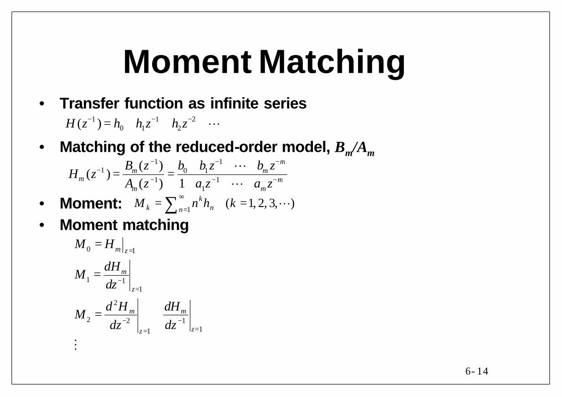
Moment Matching• Transfer function as infinite series

• Matching of the reduced-order model, Bm/Am

• Moment:• Moment matching

1 1 20 1 2( )H z h h z h z− − −= + + +L

1 11 0 1

1 11

( )( )

( ) 1

mm m

m mm m

B z b b z b zH z

A z a z a z

− − −−

− − −

+ + += =

+ + +LL

1( 1, 2, 3, )k

k nnM n h k

∞

== =∑ L

0 1

1 11

2

2 2 111

m z

m

z

m m

zz

M H

dHM

dz

d H dHM

dz dz

=

−=

− −==

=

=

= +

M

6-15

• Example 10.4 (Moment matching)

– Reduced-order model

– Moment matching

– Reduced first-order model

11 1 2 3

1 2

0.22( ) 0.22 0.154 0.1254

1 0.7 0.08z

H z z z zz z

−− − − −

− −= = + + +− −

L

1 11 0 1

1 11

( )( )

( ) 1m

mm

B z b b zH z

A z a z

− −−

− −

+= =

+

0 11

1

1 0 11 2

1 1

2 21 0 1 1

2 311

11

4.9091(1 )

( )2 39.1074(1 )

m z

m

z

m

z

b bH

a

dH a b bdz a

d H a b a bdz a

=

−=

−=

+= =

+

− += =

+

−= =+

M

11

1 1

0.0149 0.1858( )

1 0.7993z

H zz

−−

−

+=

−

6-16

Pade Approximation• Truncated Taylor series expansion

• Pade approximation

• Example 10.5

– First order:

– Second order:

2 10 1 2 1

( )( ) ( )

( )m

m mB s

G s G s g g s g sA s

−−= ≈ = + + +L

( ) ( ) ( )m m mB s G s A s=

2 33 2

( ) 458( ) 2 2.262 2.2876 2.2898

( ) 31 259 229Y s

G s s s sU s s s s

= = ≈ − + − ++ + +

L

1 1 0 1( ) / ( ) /(1 )B s A s b a s= +

22 2 0 1 1 2( ) / ( ) ( )/(1 )B s A s b b s a s a s= + + +

0 1 1 1/(1 ) 2 2.262 ( ) / ( ) 2 /(1 1.131 )b a s s B s A s s+ = − ⇒ = +

2 2 30 1 1 2

22 2

( ) /(1 ) 2 2.262 2.2876 2.2898

( ) / ( ) (2 0.0645 )/(1 1.0987 0.0989 )

b b s a s a s s s s

B s A s s s s

+ + + = − + −

⇒ = − + +

6-17

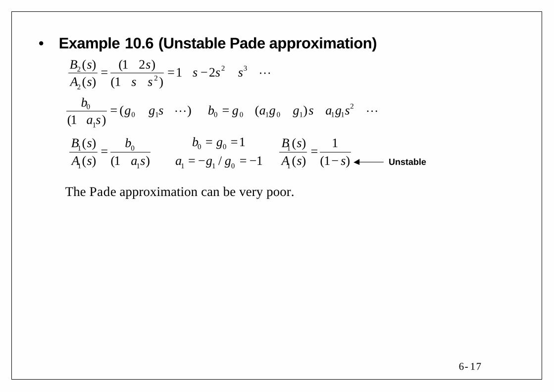
• Example 10.6 (Unstable Pade approximation)

The Pade approximation can be very poor.

2 322

2

( ) (1 2 )1 2

( ) (1 )B s s

s s sA s s s

+= = + − + +

+ +L

0 001 1

1 1 01 1 1

1( ) ( ) 1/ 1( ) (1 ) ( ) (1 )

b gbB s B sa g gA s a s A s s

= == ⇒ ⇒ = = − = −+ −

200 1 0 0 1 0 1 1 1

1

( ) ( )(1 )

bg g s b g a g g s a g s

a s= + + ⇒ = + + + +

+L L

Unstable

6-18

Describing Function Analysis• Analysis of Linear systems

– Laplace and Fourier transforms

• Describing function analysis– Extension of frequency analysis to nonlinear systems– Based on harmonic analysis– Assumptions

• Assumed periodic solution is sufficiently close to sinusoidal oscillationy(t)=Csin(ωt).

• The nonlinearity can be represented by u=n(x,x’).

– Fourier series expansion( )

0 1 1 1

1( ) cos( ) sin( )

2ki kx

k k kk k kf x a a kx a kx c e ϕ∞ ∞ ∞ +

= = == + + =∑ ∑ ∑

/ 2 /2

/2 /2

2 2where ( )cos( ) , ( )sin( )

T T

k kT Ta f t kt dt b f t kt dt

T T− −= =∫ ∫

2 2 , arctan( / )k k k k k kc a b a bϕ= + =

6-19

– Description of periodic oscillation with input amplitude C

• Describing function N(C) is obtained as the amplitude dependent gain|N(C)| and its phase shift ϕ1(ω) for the nonlinear elements.

• Harmonics caused by nonlinearities are ignored in describing functionanalysis

• Characteristic equation

– If the Nyquist curves of G0(iω) and −1/N(C) cross, it indicates the possibleexistence of a limit cycle with amplitude C and frequency ω0.

11 1 1( )( ) ic C b ia

N C eC C

ϕ += =

/ 2

/ 2

/ 2

/ 2

2where ( sin , cos )cos( ) ,

2( sin , cos )sin( )

T

k T

T

k T

a n C t C t kt dtT

b n C t C t kt dtT

ω ω ω

ω ω ω

−

−

=

=

∫

∫

Describing function

0( )

( ) ( ) ( ) ( ) ( , ) 0, /( )

B sG s A p x t B p n x x p d dt

A s= ⇒ + = ≡&

0(1 ( ) ( )) ( ) 0G p N C x t+ =

0 ( ) 1/ ( )G p N C= −

6-20

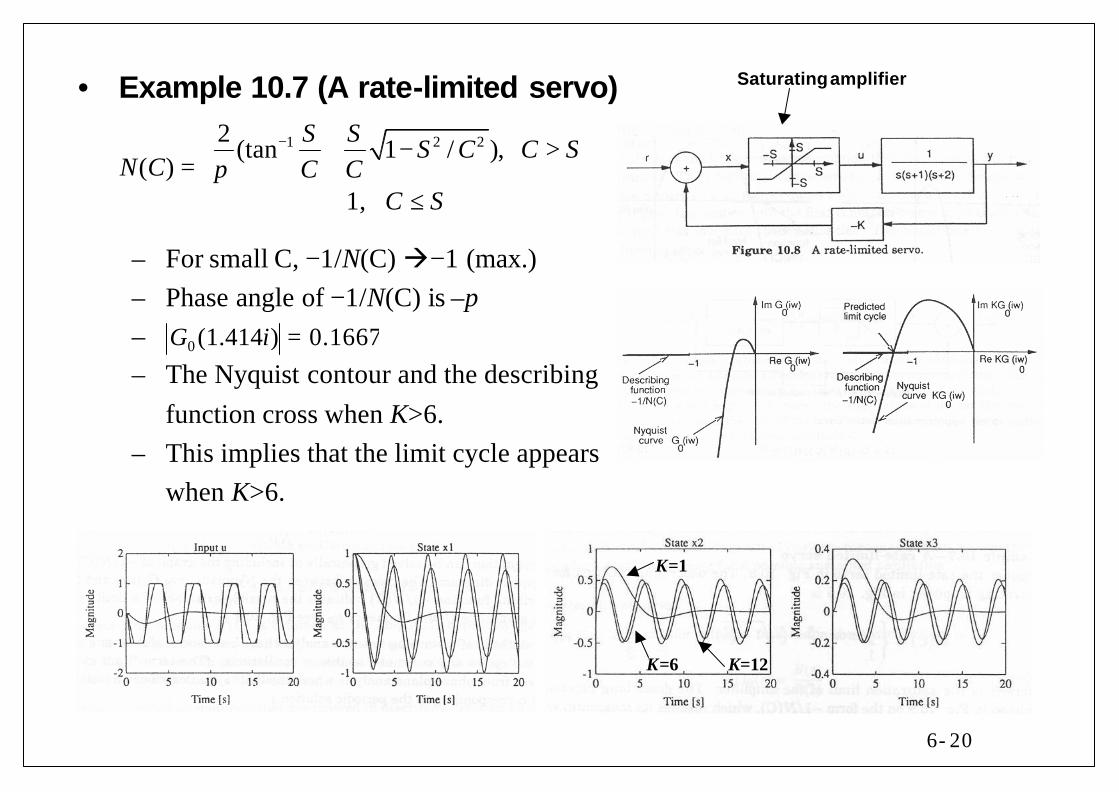
• Example 10.7 (A rate-limited servo)

– For small C, −1/N(C)à−1 (max.)– Phase angle of −1/N(C) is –π–– The Nyquist contour and the describing

function cross when K>6.– This implies that the limit cycle appears

when K>6.

1 2 22(tan 1 / ),

( )1,

S SS C C S

N C C CC S

π− + − >=

≤

Saturating amplifier

0 (1.414 ) 0.1667G i =

K=1

K=6 K=12

6-21

• Condition of application– Assumption: the input to nonlinearity is a sinusoid– Linear element is usually low-pass: higher harmonics will be attenuated– The conditions

•• G0(s) must not have any imaginary poles s=ik.• The function n(x,x’) should have finite partial derivatives w.r.t. x and x’

and must not be an explicit function of time.• The zero-order coefficient c0=0 of n(x,x’).

– If the prerequisites are not satisfied, the describing function analysis maypredict oscillations that do not exist and may fail to predict periodicsolutions that indeed do exist.

0 0 0( ) ( ) for 2,3, and ( ) 0 asG ik G i k G ik kω ω ω= → → ∞= L

6-22

• Example 10.8 (Pulse-width modulation, PWM)– PWM leads to asymmetric inputs– It requires more complicated analysis with a nonzero constant term c0 of

the describing function.– Consider a PWM system with switching nonlinearity

• The pulse-width modulating signal z is often a sawtooth-shaped signalof high frequency.

• The pulse-width modulated signal is a square wave with nonzero mean.

– If the modulating frequency ω z is high compare to G0(s), the highfrequency components deriving from z are efficiently absorbed by thelow-pass link G0(s).

0 1( ) ( , ) (1/ ) ( )u t n v v z x t n z= ≈ +& (n1 is the ordinary describing function terms)

0( ) (1/ ) ( )u t z x t≈ (linearized form)

6-23

Balanced Model Reduction inIdentification

• Usage of balanced model reduction– Further reduction from a linearized model– Identify a reduced-order linear model

• Identification assisted with model reduction– Estimation of high-order model (with sufficient excitation)– Model reduction with elimination of less important states

• Example 10.9 (Model reduction in identification)

– Identification as first-order model: biased

– Estimate 10-th order model, then reduce to first-order model

1: 0.9 0.1 ( 1)k k kS y y u d d+ = + + =

1 0.9838 0.2638k k ky y u+ = +

0.2912 0.0192k k ky x u= −1 0.9466 0.2912k k kx x u+ = + 0.0192 0.1029

( ) ( )0.9466z

Y z U zz

− +⇔ =

−

6-24

• Example 10.10 (An impulse response test)– Impulse response data

– State-space model for impulse response, g

– Balanced model reduction with n=2

( ) 1.2 (0.5) 0.2 (0.75)t tg t = ⋅ + ⋅

1

0 0 0 0 11 0 0 0 00 1 0 0

00 0 1 0 0

k k kx x u+

= +

LLO M

MO O O ML

( )0 1 1k n n ky g g g g x−= LImpulse response coefficients

( ) 1.38 (0.523) 0.38 (0.703)t tg t = ⋅ + ⋅