Lecture 6: Markov Chain Monte Carlo - NBI

University of Copenhagen Niels Bohr Institute

D. Jason Koskinen [email protected]

Photo by Howard Jackman

Advanced Methods in Applied Statistics Feb - Apr 2019

Lecture 6: Markov Chain Monte Carlo

mailto:[email protected]?subject=

D. Jason Koskinen - Advanced Methods in Applied Statistics

• Bayes Recap

• Markov Chain

• Markov Chain Monte Carlo

Outline

!2

*Material drawn from R. M. Neal, C. Chan, and wikipedia


• We have Bayes’ theorem

• or sometimes

• Let B be the observed data and A be the model/theory parameters, then we often want the P(A|B); the posterior probability distribution conditional on having observed B.

Bayes Theorem

!3

P (A|B) =P (B|A)P (A)

P (B)

P (A|B) =P (B|A)P (A)Pi P (B|Ai)P (Ai)

P (B|A)P (A)RP (B|A)P (A)dA

(Continuous)(Discrete)


• One can solve the respective conditional probability equations for P(A and B) and P(B and A), setting them equal to give Bayes’ theorem:

• In the previous lecture we avoided dealing with the marginal likelihood, i.e. the normalizing constant, because it does not depend on the parameter(s) A. But it is an important value in order to get an accurate posterior distribution which is a useable probability.

Bayes’ Theorem

!4

P (A|B) =P (B|A)P (A)

P (B)

posterior

prior

likelihood

marginal likelihood

posterior / prior⇥ likelihood


• Beta Distribution

• for a continuous random variable (x) given parameters α and β:

• Expectation and Variance:

• Often used to represent a PDF of continuous random variables which are non-zero only between finite limits

Common PDF (Beta Distribution)

!5

f(x;↵,�) =�(↵ + �)�(↵)�(�)

x↵�1(1� x)��1

E[x] =↵

↵ + �V [x] =

↵�

(↵ + �)2(↵ + � + 1)


• Coin flipping bias with n throws/flips, but now in Bayesian where we want the prob. of coming up heads (θ)

• Likelihood is the standard binomial

• Prior here is the beta-distribution with 𝝰=5 and 𝝱=17

• Plot the priors, likelihood, and posteriors for n=100 coin flips with heads=66

• This is the repeat of a previous lecture’s exercise, but now with different priors, likelihoods, and posteriors

• Normalize them to be on the same scale for plotting

• Does not have to be normalized to 1

• Normalizations for a binomial likelihood (and posterior distributions using a binomial likelihood) are summations instead of integrals

Exercise #1

!6

(continued on next slide)


• Remember that for Bayesian analyses we include all possible values of the parameter, i.e. θ

• This means for the posterior, it will not be calculated at a single value of θ, but over a suitable range of 0-1

• The likelihood PDF is now technically a ‘probability mass function’ because it is discrete

• Many packages have the binomial PMF (scipy.stats.binom.pmf( k, n, p)) • I’ll point out again that the above scipy function is a calculation for a single

probability p, but we want to scan θ over a range from 0-1

• Don’t worry about the marginal likelihood in the denominator, yet.

Exercise #1 (cont.)

!7


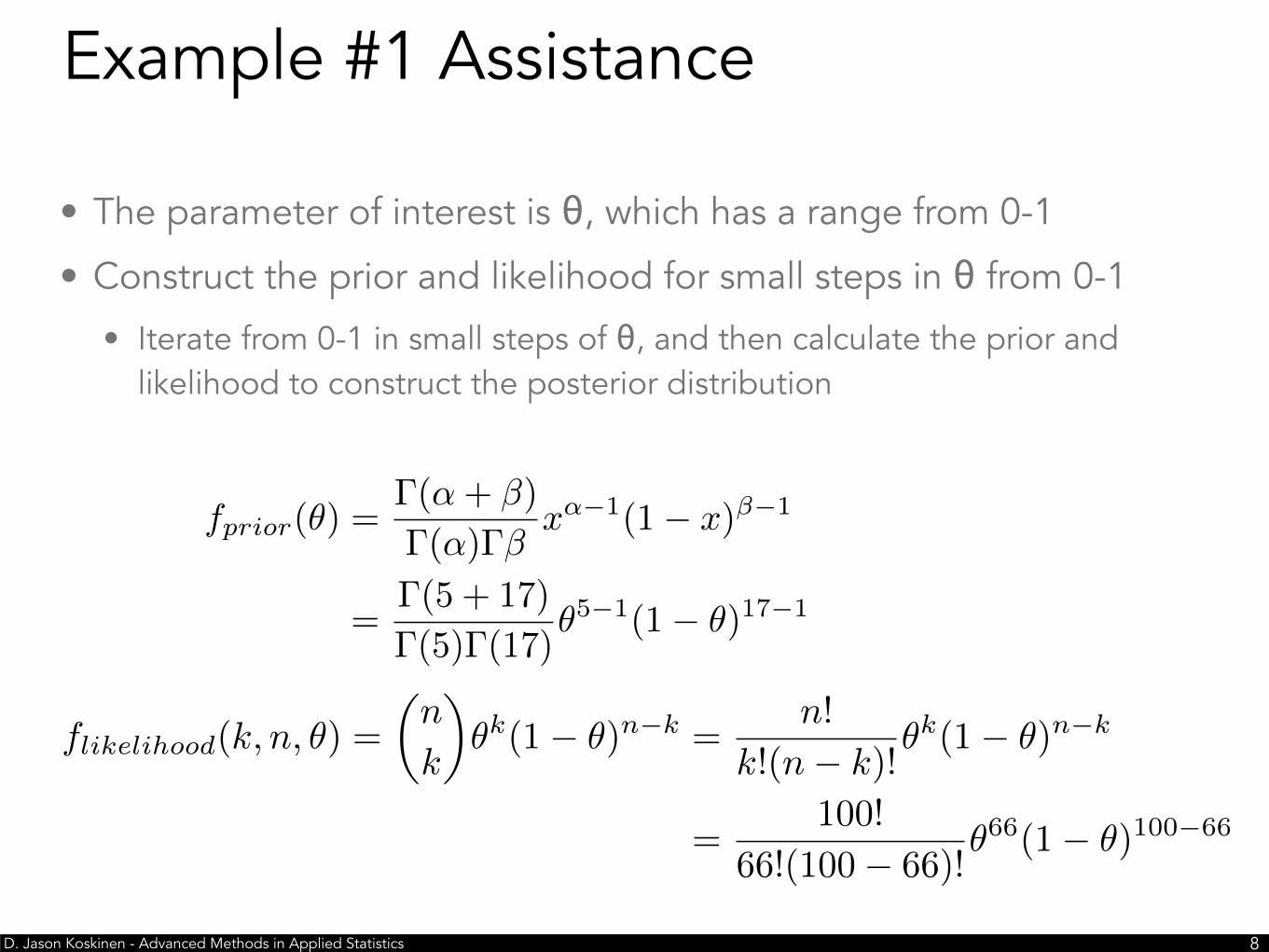
• The parameter of interest is θ, which has a range from 0-1

• Construct the prior and likelihood for small steps in θ from 0-1

• Iterate from 0-1 in small steps of θ, and then calculate the prior and likelihood to construct the posterior distribution

Example #1 Assistance

!8

fprior(✓) =�(↵+ �)

�(↵)��x↵�1(1� x)��1

=�(5 + 17)

�(5)�(17)✓5�1(1� ✓)17�1

<latexit sha1_base64="YbXLHKt+laq0DxLy2T7jZuPNHpQ=">AAACwXicbVHLbhMxFPUMrxJeKawQmxERaKKq0RgahQ2iogvKrkikrZRJojuOp7FqeyzbgxpZ81V8DV/CFs9DgqRcydLxOb7H18eZ4szYJPkVhHfu3rv/YO9h79HjJ0+f9fefn5ui1IROScELfZmBoZxJOrXMcnqpNAWRcXqRXZ/U+sUPqg0r5He7UXQu4EqynBGwnlr2f+ZLpzQrdBWndk0tDKO3H9NcA3HpFxAC4hS4WsNBmtVitc0O251rxKq6WbiWP8RVjA9vhotW8ds07e34jg/w5K/fuLOKa7KdZOHGrU832MLhSeO07A+SUdJUdBvgDgxQV2fL/u90VZBSUGkJB2NmOFF27kBbRjitemlpqAJyDVd05qEEQc3cNeFW0RvPrKK80H5JGzXsvx0OhDEbkfmTAuza7Go1+T9tVtr8w9wxqUpLJWkvykse2SKqfypaMU2J5RsPgGjmZ43IGnyC1v/n1i1ZJrYe4QhIQnnV80nh3Vxug/N3I/x+lHw7Ghx/7jLbQ6/QaxQjjCboGJ2iMzRFJHgZfApOg6/hSchCFer2aBh0PS/QVoXuD6X+2Dc=</latexit>

flikelihood(k, n, ✓) =

✓n

k

◆✓k(1� ✓)n�k =

n!

k!(n� k)!✓k(1� ✓)n�k

=100!

66!(100� 66)!✓66(1� ✓)100�66

<latexit sha1_base64="h8aiv/7oLoQoCVifE/hN3QppCOw=">AAACvXicfZFda9swFIZldx9d9pV27Go3ysKGC02w2+INRlnZB+yyg6UtxGmQleNGWJaMJG8Eod+037NfstspiRlNO3ZA8PKe83CkV3nNmTZx/CsIt+7cvXd/+0Hn4aPHT552d3bPtGwUhRGVXKqLnGjgTMDIMMPholZAqpzDeV5+XPbPv4PSTIpvZlHDpCJXghWMEuOtafdnMbWclZ6fSzlzUbkv9jMzB0P2jq3IqHc14NKtvUtbuigZtAOXVgxKh18f46xQhFrRc7bsRd7c6/0HyLLOXySJYw+laS/yapCm18A03SDXfTft9uNhvCp8WySt6KO2Tqfd39lM0qYCYSgnWo+TuDYTS5RhlIPrZI2GmtCSXMHYS0Eq0BO7CtbhV96Z4UIqf4TBK/c6YUml9aLK/WRFzFzf7C3Nf/XGjSneTiwTdWNA0PWiouHYSLz8JTxjCqjhCy8IVczfFdM58YkZ/5cbW/K82niEpURQ4K7jk0pu5nJbnB0Mk8Nh/PWof/KhzWwbvUAvUYQS9AadoC/oFI0QDZ4H74JPwefwfQghD8V6NAxa5hnaqPDHHxsQ1So=</latexit>


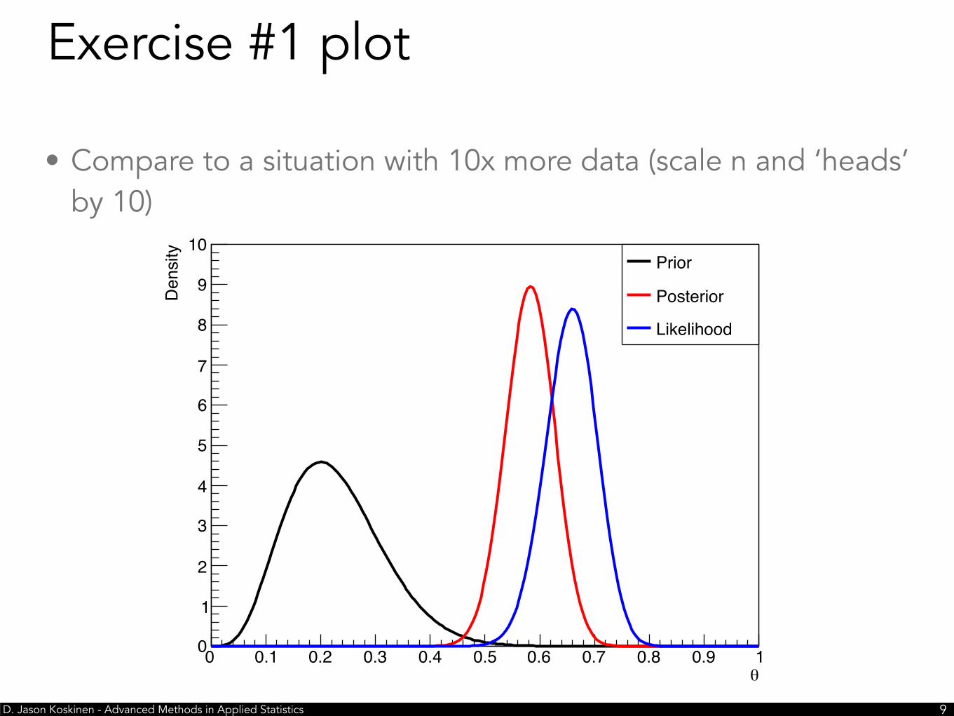
• Compare to a situation with 10x more data (scale n and ‘heads’ by 10)

Exercise #1 plot

!9

θ0 0.1 0.2 0.3 0.4 0.5 0.6 0.7 0.8 0.9 1

Density

0

1

2

3

4

5

6

7

8

9

10Prior

Posterior

Likelihood


• With 10x more statistics, an obvious feature pops up, i.e. that as n⇾infinity the maximum a posterior (MAP) approaches the maximum likelihood estimator (MLE), irrespective of the prior

Exercise #1 (cont.)

!10

θ0 0.1 0.2 0.3 0.4 0.5 0.6 0.7 0.8 0.9 1

Density

0

5

10

15

20

25

30

35Prior

Posterior

Likelihood


• The previous example had only 1 parameter (θ) and 1 prior, so it is not computationally intensive to produce the marginal likelihood, prior, or likelihood for all relevant values by summation/integration. But, when dealing with more parameters, the computational load approx. increases exponentially with the number of parameters.

• For summation — or integration via Monte Carlo sampling — the number of points (n) grows as if n points are used to cover each parameter (d)

Numerical Limitations

!11

O(nd)


• In order to estimate joint likelihood probability functions, e.g. likelihoods with multiple parameters, we can use Monte Carlo integration and sampling to estimate the distribution

• In order to estimate Bayesian posterior distributions, it would be nice to use the same strategy when confronted by higher dimension integrals, e.g. for the marginal likelihood. But, it is often difficult — sometimes impossible — to sample from the posterior distribution effectively using the same approach as what we can do for likelihood distributions

• Solution is to use Markov chains which converge to the posterior distribution

Posterior Distribution Sampling

!12


• A Markov chain is a stochastic process (random walk) of steps or state transitions that is only conditional on the current step/state. The transition from the current state to the next state is often, but not always, governed by a probability

• More math-like: the conditional transition of Xt+1 only depends on Xt and not X1, X2,…, Xt-1

• In this way Markov chains have no memory or dependence on previous transitions

Markov Chain

!13

P (Xt+1|X1, X2, ...,Xt) = P (Xt+1|Xt)

new state = f(current state, transition probability)


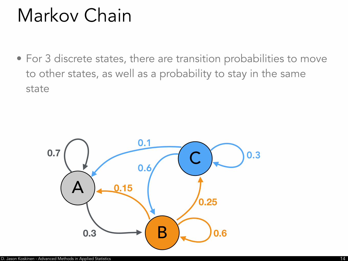
• For 3 discrete states, there are transition probabilities to move to other states, as well as a probability to stay in the same state

Markov Chain

!14

A

B

C

0.6

0.6

0.10.3

0.250.15

0.3

0.7


• Transition probabilities can also be shown in matrix notation

• Visually, it should be clear that the next transition is conditional only on the current state

Markov Chain

!15

A

B

C

0.6

0.6

0.10.3

0.250.15

0.3

0.7

P (A ! A) = 0.7

P (A ! B) = 0.3

P (A ! C) = 0.0

P (B ! A) = 0.15

P (B ! B) = 0.60

P (B ! C) = 0.25

P (C ! A) = 0.1

P (C ! B) = 0.3

P (C ! C) = 0.6


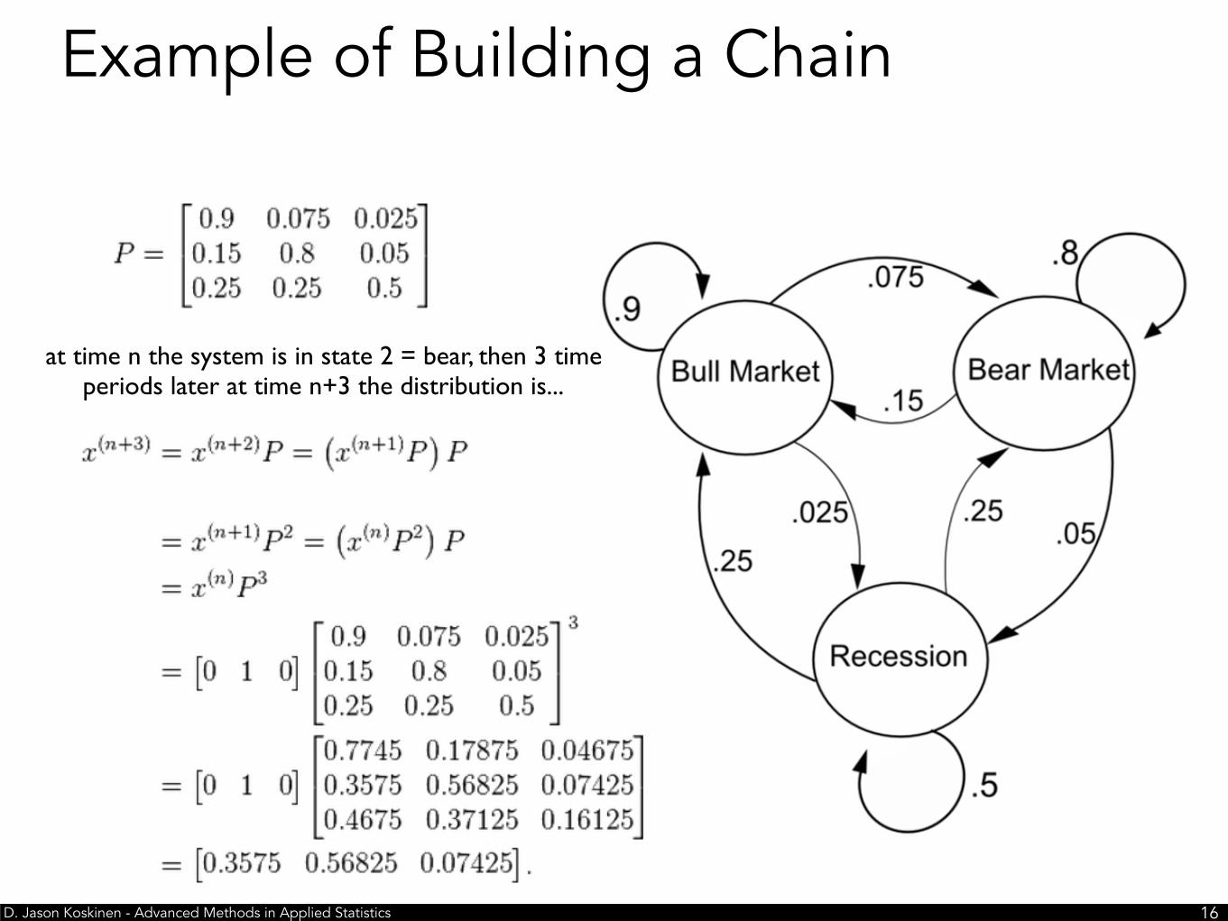
Example of Building a Chain

!16

at time n the system is in state 2 = bear, then 3 time periods later at time n+3 the distribution is...


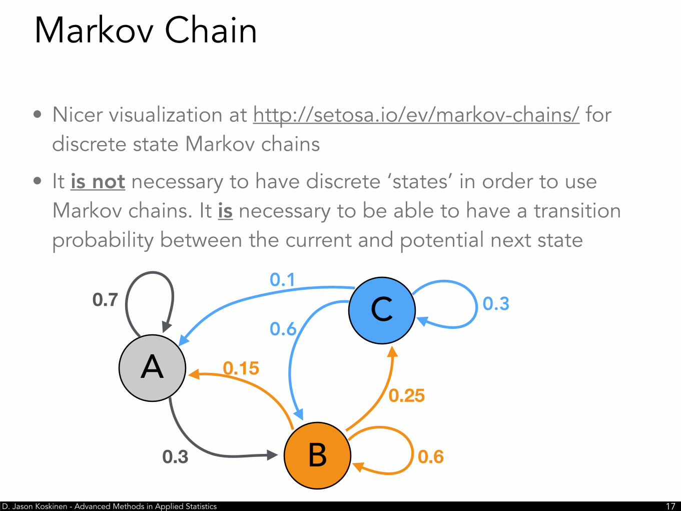
• Nicer visualization at http://setosa.io/ev/markov-chains/ for discrete state Markov chains

• It is not necessary to have discrete ‘states’ in order to use Markov chains. It is necessary to be able to have a transition probability between the current and potential next state

Markov Chain

!17

A

B

C

0.6

0.6

0.10.3

0.250.15

0.3

0.7

http://setosa.io/ev/markov-chains/


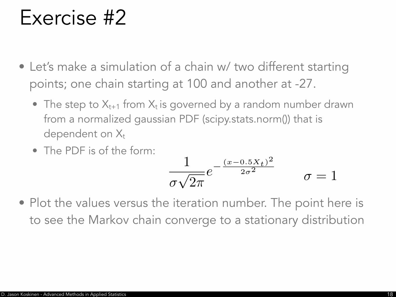
• Let’s make a simulation of a chain w/ two different starting points; one chain starting at 100 and another at -27.

• The step to Xt+1 from Xt is governed by a random number drawn from a normalized gaussian PDF (scipy.stats.norm()) that is dependent on Xt

• The PDF is of the form:

• Plot the values versus the iteration number. The point here is to see the Markov chain converge to a stationary distribution

Exercise #2

!18

1

�p2⇡

e�(x�0.5Xt)

2

2�2� = 1


• After maybe 5-10 iterations from the starting point the chains look to converge to some stationary behavior

Exercise #2 (plots)

!19

Markov Chain Iteration0 20 40 60 80 100

20−

0

20

40

60

80

100

The samples before convergence are commonly known as ‘burn-in samples’ and are not often included

when estimating the posterior distribution. They’re generally just

discarded and understood as the cost of using Markov

Chain Monte Carlos.


• When zoomed in we see that there is some stable distribution with some random scatter which the chain converges to irrespective of the starting point

Exercise #2 (plots)

!20Markov Chain Iteration

0 20 40 60 80 10010−

8−

6−

4−

2−

0

2

4

6

8

10


• Assuming that the distribution that this chain converges to is a gaussian, use the samples after some number of iterations (~10) to estimate the mean and sigma

Exercise #2 (extra)

!21Markov Chain Iteration

0 20 40 60 80 10010−

8−

6−

4−

2−

0

2

4

6

8

10


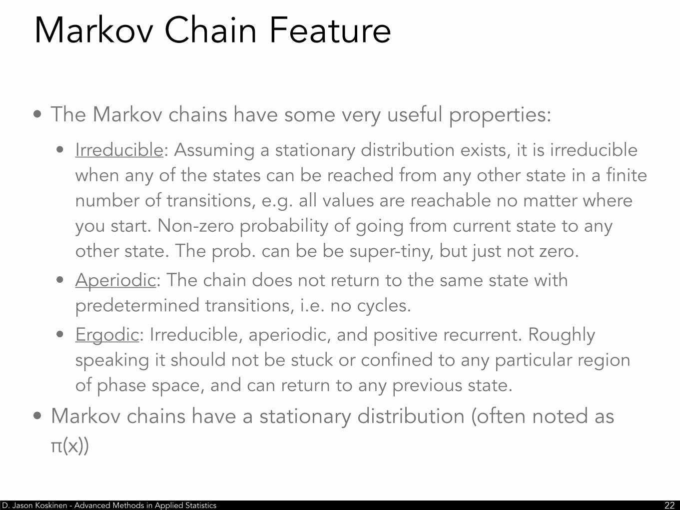
• The Markov chains have some very useful properties:

• Irreducible: Assuming a stationary distribution exists, it is irreducible when any of the states can be reached from any other state in a finite number of transitions, e.g. all values are reachable no matter where you start. Non-zero probability of going from current state to any other state. The prob. can be be super-tiny, but just not zero.

• Aperiodic: The chain does not return to the same state with predetermined transitions, i.e. no cycles.

• Ergodic: Irreducible, aperiodic, and positive recurrent. Roughly speaking it should not be stuck or confined to any particular region of phase space, and can return to any previous state.

• Markov chains have a stationary distribution (often noted as π(x))

Markov Chain Feature

!22


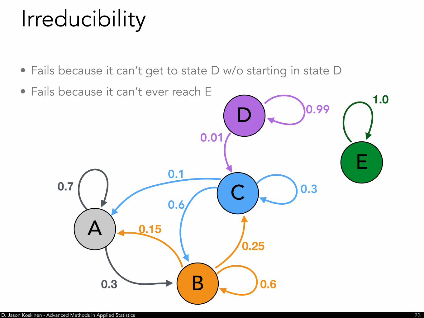
• Fails because it can’t get to state D w/o starting in state D

• Fails because it can’t ever reach E

Irreducibility

!23

A

B

C

0.6

0.6

0.10.3

0.250.15

0.3

0.7

D 0.99

0.01

E

1.0


• So how does a Markov chain help with establishing Bayesian posterior distributions?

• Well, Markov chains will asymptotically approach a stable distribution, and we can give the Markov chain a distribution that is representative of the posterior. Remember that,

• So using Markov Chain Monte Carlo, the chain can start at points that are not typical of the actual posterior (which we may not know well), but after enough Monte Carlo iterations it should converge to the posterior.

• Now we need to find transition schemes that cause the chain to converge to the stable or invariant posterior distribution.

Markov Chains for Bayes’ Stuff

!24

posterior / prior⇥ likelihood


• Thankfully, a host of Markov chain methods have already been produced, so it is unnecessary to derive our own for most problems

• While there are many types of Markov chains, there are at least two that you are likely to encounter

• Metropolis-Hastings, which is actually a more general case than the original Metropolis algorithm

• Gibbs sampling

• We will cover Metropolis-Hastings to get a feel for what is happening with the chains, but you are encouraged to use other Markov chain techniques too

Monte Carlo Markov Chains (MCMC)

!25


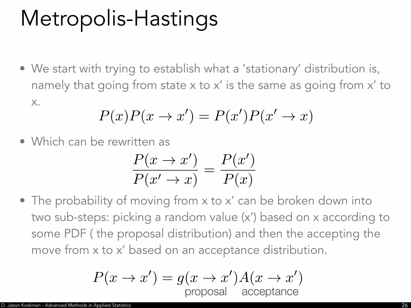
• We start with trying to establish what a ‘stationary’ distribution is, namely that going from state x to x’ is the same as going from x’ to x.

• Which can be rewritten as

• The probability of moving from x to x’ can be broken down into two sub-steps: picking a random value (x’) based on x according to some PDF ( the proposal distribution) and then the accepting the move from x to x’ based on an acceptance distribution.

Metropolis-Hastings

!26

P (x)P (x ! x0) = P (x0)P (x0 ! x)

P (x ! x0)

P (x0 ! x)=

P (x0)

P (x)

P (x ! x0) = g(x ! x0)A(x ! x0)proposal acceptance


• Thus,

• becomes,

• I could have used xt instead of just x, but x’ is not xt+1. x’ is the candidate for transition

• P(x) is often written as π(x) to reflect that it is the stationary distribution

Metropolis-Hastings

!27

P (x ! x0)

P (x0 ! x)=

P (x0)

P (x)

A(x ! x0)

A(x0 ! x)=

P (x0)g(x0 ! x)

P (x)g(x ! x0)

=P (x0)g(x|x0)

P (x)g(x0|x)


• Let’s take a moment to think about the acceptance ratio

• If r ≥ 1, it means that the move from x to x’ is a transition to a more/equally likely state and that it should be accepted, i.e. xt+1=x’

• If r < 1, there is a non-zero probability that the transition is made, i.e. xt+1=x’, but only in proportion to the probability r. Otherwise, the transition is rejected and we re-sample at the current point, i.e. xt+1=x. • This way the Markov chain does not get stuck in a local area because it always has some

probability of a transition to a less probably state or can make a large (but unlikely) ‘jump’ that leads to a more probable state

• When the Markov chain converges to the stationary distribution it will effectively start to sample the posterior distribution, which is exactly what we want

Metropolis-Hastings

!28

r =A(x ! x0)

A(x0 ! x)=

P (x0)g(x|x0)

P (x)g(x0|x)


• Metropolis-Hastings corrects for a bias which could be introduced from having an asymmetric proposal PDF, e.g. g(x|x’)

• We might want an asymmetric proposal PDF because we will knowingly start the Markov chain always above/below the maximum a posteriori (MAP). Thus, the Markov chain is likely to converge quicker if the transitions in either the +/- direction are larger versus the opposite direction.

• But, when the Markov chain does converge, we want it sample the posterior distribution properly. So we need to include the probability that transitions from proposal function will not be symmetric, i.e. the probability of g(x|x’) ≠ g(x’|x).

Quick Note

!29


• Having a proposal function (PDF) which is narrow can translate into many iterations before converging, which is inefficient

• A proposal PDF which is large can cause the Markov chain to ‘jump’ over the desired posterior distribution area, and converge in some other region

• Tuning MCMCs is often necessary to balance these two competing issues, and rerunning the MCMC multiple times helps to establish that you have actually found the posterior distribution

• Just like minimizing for negative likelihoods there are no concrete rules for establishing if the MCMC has found the invariant global posterior distribution

Proposal Function

!30


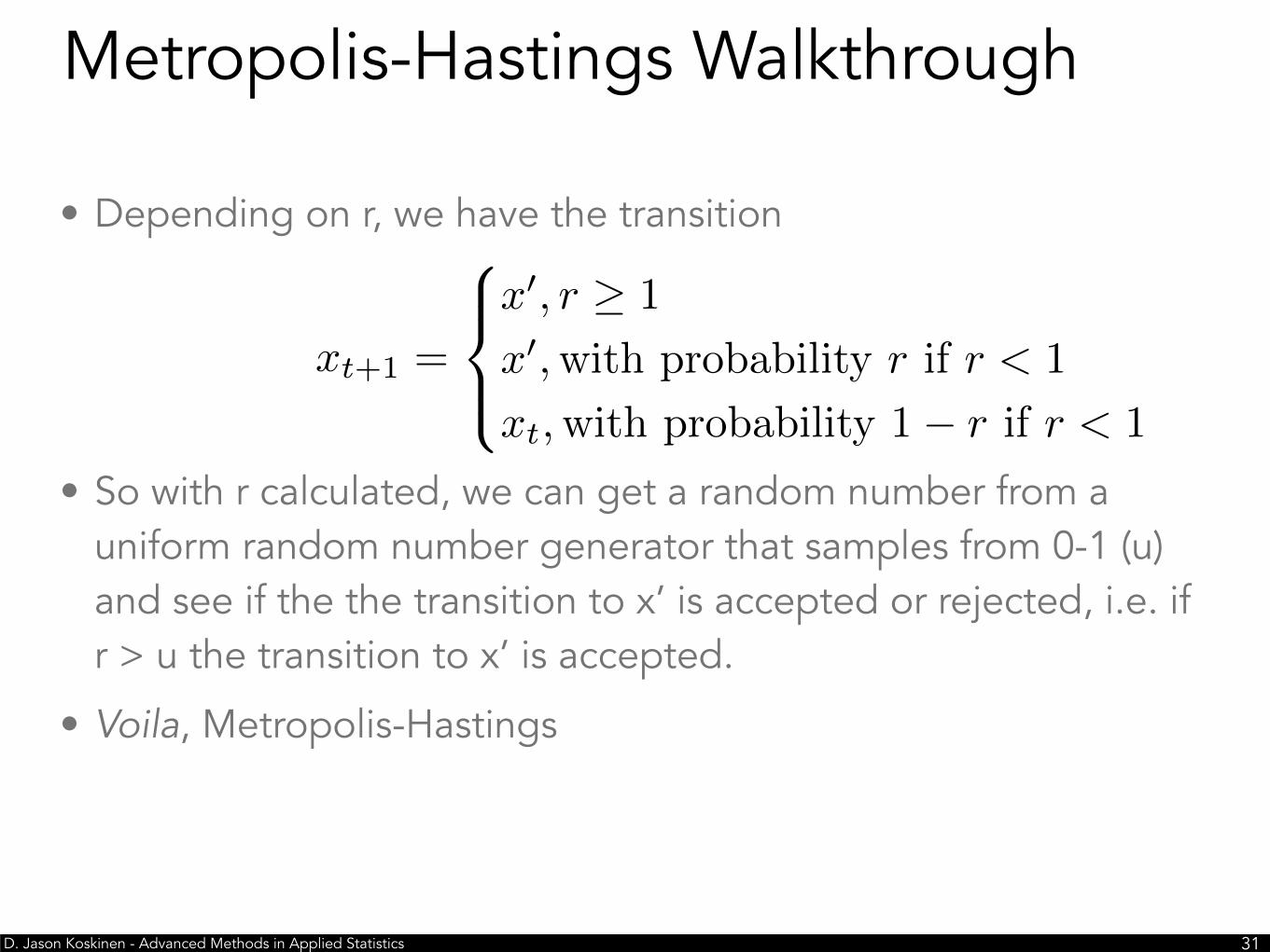
• Depending on r, we have the transition

• So with r calculated, we can get a random number from a uniform random number generator that samples from 0-1 (u) and see if the the transition to x’ is accepted or rejected, i.e. if r > u the transition to x’ is accepted.

• Voila, Metropolis-Hastings

Metropolis-Hastings Walkthrough

!31

xt+1 =

8><

>:

x0, r � 1

x0,with probability r if r < 1

xt,with probability 1� r if r < 1


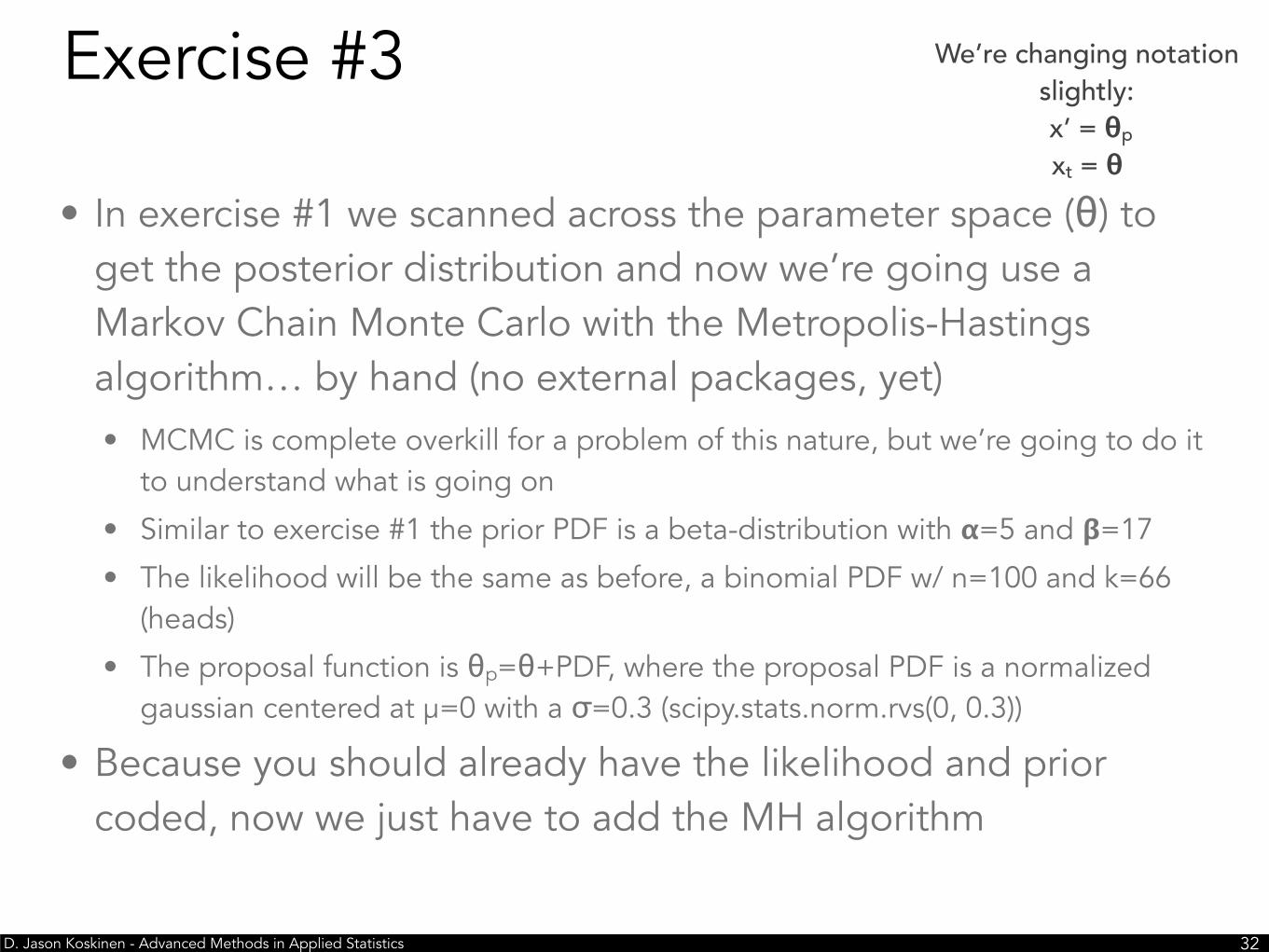
• In exercise #1 we scanned across the parameter space (θ) to get the posterior distribution and now we’re going use a Markov Chain Monte Carlo with the Metropolis-Hastings algorithm… by hand (no external packages, yet) • MCMC is complete overkill for a problem of this nature, but we’re going to do it

to understand what is going on

• Similar to exercise #1 the prior PDF is a beta-distribution with 𝝰=5 and 𝝱=17

• The likelihood will be the same as before, a binomial PDF w/ n=100 and k=66 (heads)

• The proposal function is θp=θ+PDF, where the proposal PDF is a normalized gaussian centered at μ=0 with a σ=0.3 (scipy.stats.norm.rvs(0, 0.3))

• Because you should already have the likelihood and prior coded, now we just have to add the MH algorithm

Exercise #3

!32

We’re changing notation slightly: x’ = θp

xt = θ


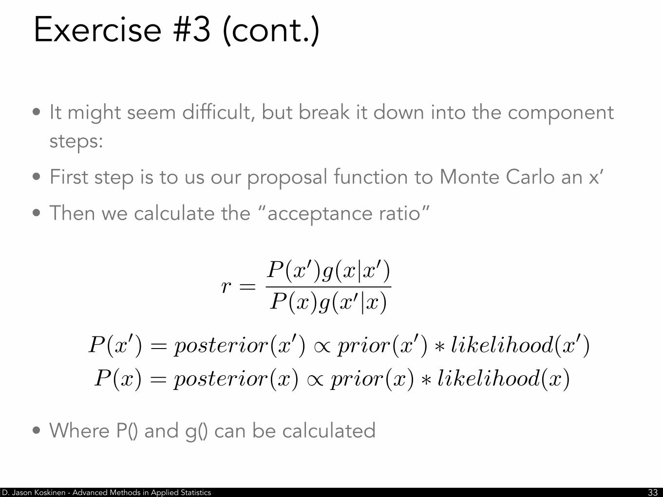
• It might seem difficult, but break it down into the component steps:

• First step is to us our proposal function to Monte Carlo an x’

• Then we calculate the “acceptance ratio”

• Where P() and g() can be calculated

Exercise #3 (cont.)

!33

r =P (x0)g(x|x0)

P (x)g(x0|x)

P (x0) = posterior(x0) / prior(x0) ⇤ likelihood(x0)

P (x) = posterior(x) / prior(x) ⇤ likelihood(x)<latexit sha1_base64="I/5fb77+rmETa3f1Wb+pPRNPZmM=">AAACP3icbVDLSgMxFM3UV62vqks3wSKoizKjgm6EohuXFewD2lIy6W0bmklCkhHL0O/wa1y40W/wC9yJO3Fn2s7CVg8Ezj33Xm7OCRVnxvr+m5dZWFxaXsmu5tbWNza38ts7VSNjTaFCJZe6HhIDnAmoWGY51JUGEoUcauHgetyv3YM2TIo7O1TQikhPsC6jxDqpnQ/Khw9Hl0oaC5pJ7Yqm0lJZiVVa42PM2cAd6EvZcXU7X/CL/gT4LwlSUkApyu38V7MjaRyBsJQTYxqBr2wrIdoyymGUa8YGFKED0oOGo4JEYFrJxNoIHzilg7tSuycsnqi/NxISGTOMQjcZEds3872x+F+vEdvuRSthQsUWBJ0e6sYcO+fjnHCHaaCWDx0hVDP3V0z7RBPqgpq9EobRjImEEkGBj3IuqWA+l7+kelIMTov+7VmhdJVmlkV7aB8dogCdoxK6QWVUQRQ9oif0gl69Z+/d+/A+p6MZL93ZRTPwvn8AsmSvbA==</latexit>


• A useful trait here is that the proposal function PDF (gaussian) is symmetric:

• So for a symmetric proposal function:

Exercise #3 (cont.)

!34

g(x|x0)

g(x0|x) = 1

g(x|x0) =1p2⇡�

e�(x�x0)2

2�2

<latexit sha1_base64="VlLjVsrR8JaDOsVDrQZsmhVKWPM=">AAACUHicbVBNTxsxFHybUj5CCwGOXFZEiPRAtBuQ4IKE4NIjSASQsiHyOm+DFdu72F6UyOz/6a/poZe2vwRu4HwgEWAky6OZsZ7fxBln2gTBf6/0Ze7r/MLiUnn52/eV1cra+qVOc0WxSVOequuYaORMYtMww/E6U0hEzPEq7p+O/Kt7VJql8sIMM2wL0pMsYZQYJ3UqJ73a4GGw8+MoShShNixspO+UsY0oY0WkWU+QAm/sxN2tDXZd9qZROH/sOVp0KtWgHozhfyThlFRhirNO5THqpjQXKA3lROtWGGSmbYkyjHIsylGuMSO0T3rYclQSgbptx7sW/rZTun6SKnek8cfq2xeWCK2HInZJQcytfu+NxM+8Vm6Sw7ZlMssNSjoZlOTcN6k/Ks7vMoXU8KEjhCrm/urTW+JqMa7emSlxLGaWsJRIirwou6bC9718JJeNerhXD873q8cn084WYRO2oAYhHMAx/IQzaAKFX/Ab/sI/74/35D2XvEn09YYNmEGp/AKhs7Vd</latexit>

g(x0|x) = 1p2⇡�

e�(x0�x)2

2�2

<latexit sha1_base64="31ULEI5KU7VmEn4CggBomJV6uHg=">AAACUHicbVBNTxsxFHyb0hLSD7blyGVFVBUORLsBqb1UitILxyCRgJQNkdd5G6zY3sX2Vonc/T/8Gg69QH9JeyvOB1IDHcnyaGas5zdJzpk2YfjLq7zYePlqs7pVe/3m7btt//2Hns4KRbFLM56pi4Ro5Exi1zDD8SJXSETC8TyZfJv7599RaZbJMzPLcSDIWLKUUWKcNPTb4/3ppx/Tg69xqgi1UWljfa2MbcY5K2PNxoKUeGmX7qHLHk4PLpul8xeeo+XQr4eNcIHgOYlWpA4rdIb+73iU0UKgNJQTrftRmJuBJcowyrGsxYXGnNAJGWPfUUkE6oFd7FoGH50yCtJMuSNNsFD/fWGJ0HomEpcUxFzpp95c/J/XL0z6ZWCZzAuDki4HpQUPTBbMiwtGTCE1fOYIoYq5vwb0irhajKt3bUqSiLUlLCWSIi9rrqnoaS/PSa/ZiI4a4elxvdVedVaFXdiDfYjgM7TgBDrQBQo3cAt3cO/99P54fyveMvp4ww6soVJ7AKC2tV0=</latexit>


Exercise #3 (cont.)

!35

• For 2000 iterations plot Markov Chain Monte Carlo samples as a function of iteration, as well as a histogram of the samples, i.e. the posterior distribution.

*This is for a different “k”, i.e. k≠66


Exercise #4

!36

• Using an external MCMC package, redo exercise 3.

• You don't have to use Metropolis-Hastings

• Do you get similar results?


• Switch to a non-symmetric proposal PDF, and see if your personally coded Metropolis-Hastings matches the results from the external package MCMC.

• Go to the lecture on “Parameter Estimation and Confidence Intervals” and replace the minimization routine with your MCMC, to see if you get the same results

Additional Exercises

!37


• Exercise 1 is revisiting Bayesian statistics w/ a new prior an likelihood

• Exercise 2 illustrates that by using a Markov chain we can start away from our ‘stable’ posterior, but Monte Carlo our way into to the stable posterior

• Exercise 3 is now using the same prior and likelihood from Exercise 1, but now instead of scanning we are using the MCMC. We can also cross-check our result with the code from Exercise 1 because the posterior is the same

• Can also check that by changing any of ‘k’ or ’n’ that the scan method matches the MCMC

Why did we do all this?

!38


• More information about Bayesian Statistics and Markov Chain Monte Carlo techniques:

• “An Introduction to MCMC for Machine Learning“ https://doi.org/10.1023/A:1020281327116

• “Markov Chain Monte Carlo Methods for Bayesian Data Analysis in Astronomy” https://doi.org/10.1146/annurev-astro-082214-122339

Additional Material

!39

https://doi.org/10.1023/A:1020281327116

https://doi.org/10.1023/A:1020281327116

https://doi.org/10.1146/annurev-astro-082214-122339


Backup

!40

Date post:	23-Jan-2022
Category:	Documents
Upload:	others
View:	1 times
Download:	0 times

Lecture 6: Markov Chain Monte Carlo - NBI

Documents