75
Spring 2009 Spring 2009 Lecture 9: Introduction to Lecture 9: Introduction to Program Analysis and Optimization Optimization
Spring 2009Spring 2009
Lecture 9: Introduction toLecture 9: Introduction to Program Analysis and
OptimizationOptimization

ead Code at o
Outline
• IntroductionIntroduction
• Basic Blocks
• Common Subexpression Elimination
C P ti • Copy Propagation
• Dead Code Elimination
• Algebraic Simplification
• Summary

Program Analysisg y
• Compile-time reasoning about run-time behavior of program – Can discover things that are always true:
“ i l 1 i th t t t ”• “x is always 1 in the statement y = x + z” • “the pointer p always points into array a” • “the statement return 5 can never execute”
– Can infer things that are likely to be true: • “the reference r usually refers to an object of class C” • “the statement a = b + c appears to execute more frequently • the statement a = b + c appears to execute more frequently
than the statement x = y + z”
– Distinction between data and control-flow properties
Saman Amarasinghe 3 6.035 ©MIT Fall 1998

•
Transformations
• Use analysis results to transform program • Overall goal: improve some aspect of program • Traditional goals:
R d b f d i i– Reduce number of executed instructions – Reduce overall code size
• Other goals emerge as space becomes more complexOther goals emerge as space becomes more complex – Reduce number of cycles
• Use vector or DSP instructions • Improve instruction or data cache hit rate
– Reduce power consumption – Reduce memory usage
Saman Amarasinghe 4 6.035 ©MIT Fall 1998
Reduce memory usage

ead Code at o
Outline
• IntroductionIntroduction
• Basic Blocks
• Common Subexpression Elimination
C P ti • Copy Propagation
• Dead Code Elimination
• Algebraic Simplification
• Summary

a o a u o u o
Control Flow Graphp
• Nodes Represent Computationp p – Each Node is a Basic Block – Basic Block is a Sequence of Instructions withq
• No Branches Out Of Middle of Basic Block • No Branches Into Middle of Basic Block • Basic Blocks should be maximal
– Execution of basic block starts with first instruction
– Includes all instructions in basic block
Saman Amarasinghe 6 6.035 ©MIT Fall 1998
• Edges Represent Control Flow

=
Control Flow Graph s = 0; p
into add(n, k) {
a = 4; i = 0;
k 0 s = 0; a = 4; i = 0; if (k == 0)
b 1
k == 0
b = 1; else
b = 2;
b = 1;b = 2;
b 2; while (i < n) {
s = s + a*b;
i < n
+ *b ;
i = i + 1; }
s = s + a*b; i = i + 1;
return s;
Saman Amarasinghe 7 6.035 ©MIT Fall 1998
return s; }
•
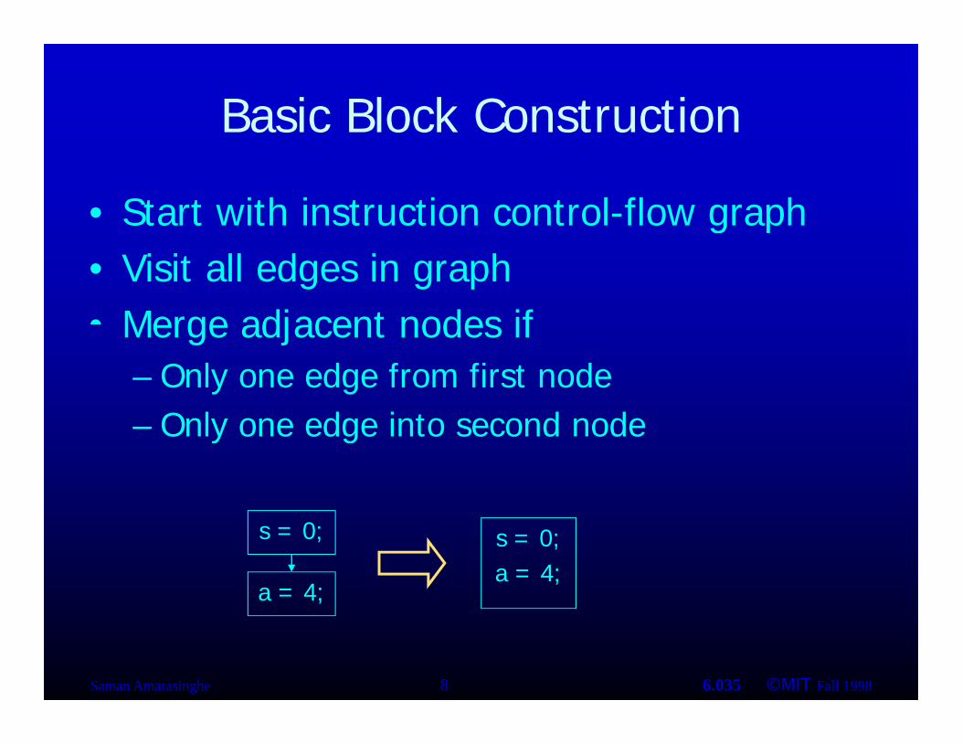
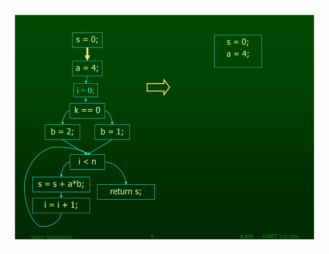
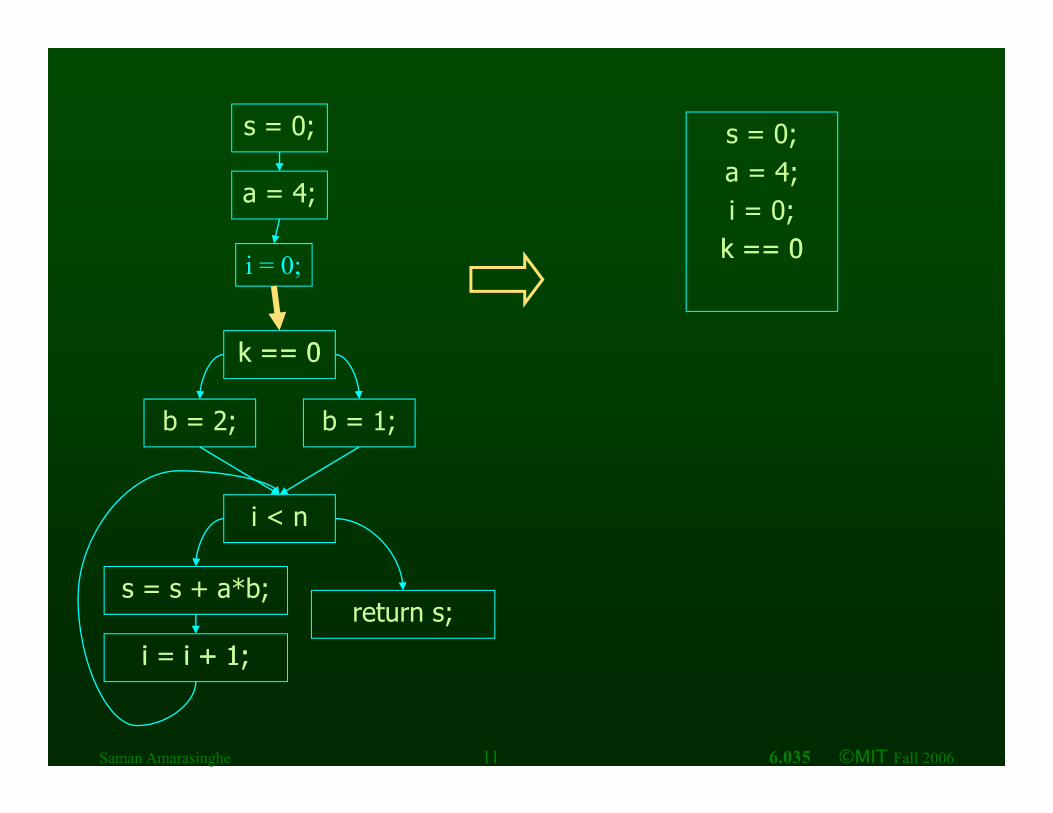
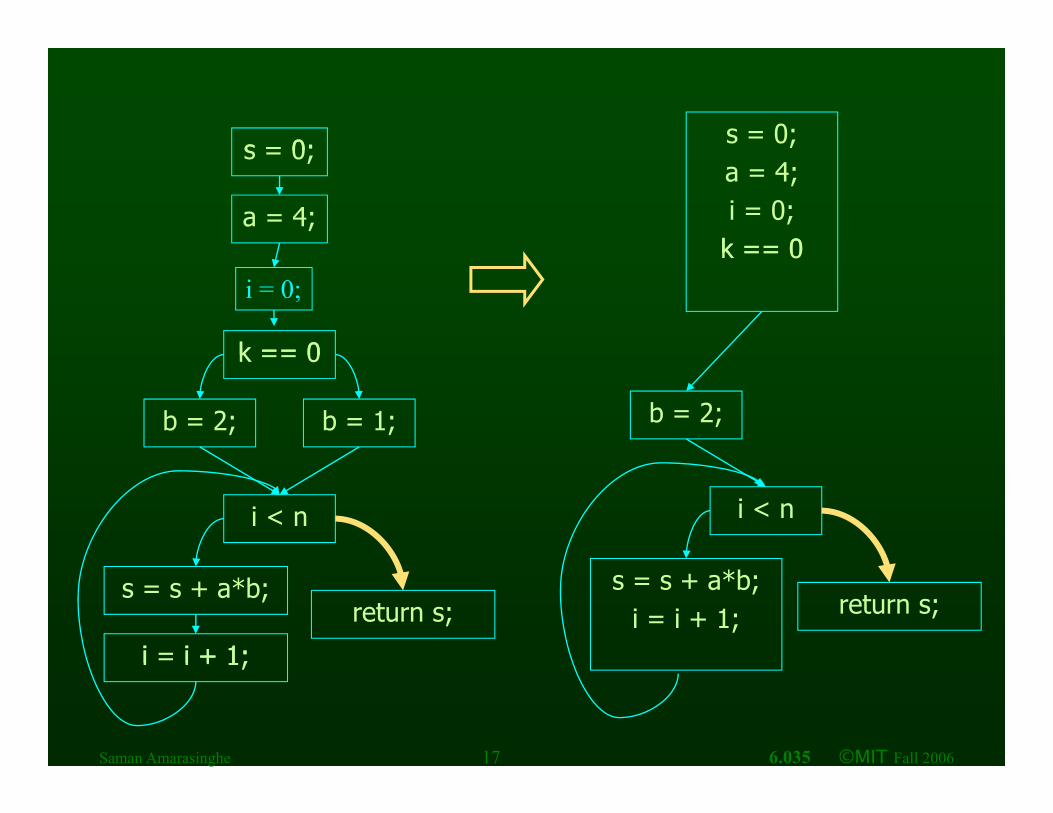
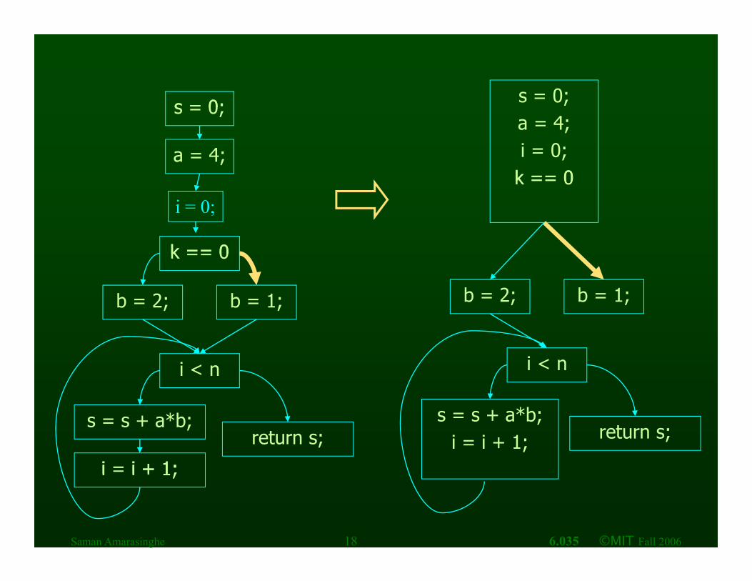
Basic Block Construction
• Start with instruction control-flow graphg p• Visit all edges in graph • Merge adjacent nodes ifMerge adjacent nodes if
– Only one edge from first node Only one edge into second node– Only one edge into second node
s = 0;
a = 4;
s = 0; a = 4;
Saman Amarasinghe 8 6.035 ©MIT Fall 1998
s = 0; s = 0;
a = 4;
a = 4;
i = 0;
k == 0k == 0
b = 1;b = 2;
i < n
s = s + a*b;
i = i + 1;
return s;
Saman Amarasinghe 9 6.035 ©MIT Fall 2006
i i + 1;

s = 0; s = 0;
a = 4; a = 4;i = 0;
i = 0;
k == 0k == 0
b = 1;b = 2;
i < n
s = s + a*b;
i = i + 1;
return s;
Saman Amarasinghe 10 6.035 ©MIT Fall 2006
i i + 1;
s = 0; s = 0;
a = 4;a = 4;i = 0;
k == 0i = 0;
k == 0
k == 0
k == 0
b = 1;b = 2;
i < n
s = s + a*b;
i = i + 1;
return s;
Saman Amarasinghe 11 6.035 ©MIT Fall 2006
i i + 1;
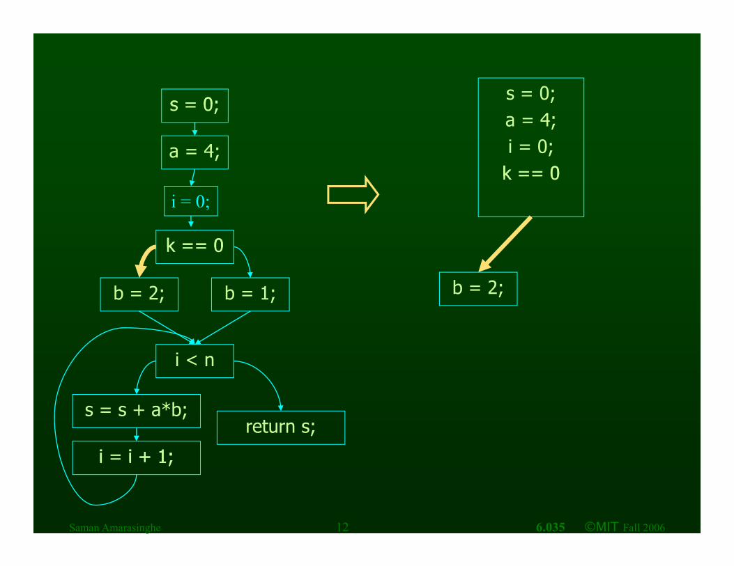
s = 0; s = 0;s = 0;
a = 4;
a = 4;i = 0;
k == 0i = 0;
k == 0
k == 0
k == 0
b = 1;b = 2; b = 2;
i < n
s = s + a*b;
i = i + 1;
return s;
Saman Amarasinghe 12 6.035 ©MIT Fall 2006
i i + 1;

s = 0; s = 0;s = 0;
a = 4;
a = 4;i = 0;
k == 0i = 0;
k == 0
k == 0
k == 0
b = 1;b = 2; b = 2;
i < n i < n
s = s + a*b;
i = i + 1;
return s;
Saman Amarasinghe 13 6.035 ©MIT Fall 2006
i i + 1;

s = 0; s = 0;s = 0;
a = 4;
a = 4;i = 0;
k == 0i = 0;
k == 0
k == 0
k == 0
b = 1;b = 2; b = 2;
i < n i < n
s = s + a*b;
i = i + 1;
return s;s = s + a*b;
Saman Amarasinghe 14 6.035 ©MIT Fall 2006
i i + 1;

s = 0; s = 0;s = 0;
a = 4;
a = 4;i = 0;
k == 0i = 0;
k == 0
k == 0
k == 0
b = 1;b = 2; b = 2;
i < n i < n
s = s + a*b;return s;
s = s + a*b;i = i + 1;
Saman Amarasinghe 15 6.035 ©MIT Fall 2006
i = i + 1;

s = 0; s = 0;s = 0;
a = 4;
a = 4;i = 0;
k == 0i = 0;
k == 0
k == 0
k == 0
b = 1;b = 2; b = 2;
i < n i < n
s = s + a*b;
i = i + 1;
return s;s = s + a*b;
i = i + 1;
Saman Amarasinghe 16 6.035 ©MIT Fall 2006
i i + 1;
s = 0; s = 0;s = 0;
a = 4;
a = 4;i = 0;
k == 0i = 0;
k == 0
k == 0
k == 0
b = 1;b = 2; b = 2;
i < n i < n
s = s + a*b;
i = i + 1;
return s;s = s + a*b;
i = i + 1; return s;
Saman Amarasinghe 17 6.035 ©MIT Fall 2006
i i + 1;
s = 0; s = 0;s = 0;
a = 4;
a = 4;i = 0;
k == 0i = 0;
k == 0
k == 0
k == 0
b = 1;b = 2; b = 1;b = 2;
i < n i < n
s = s + a*b;
i = i + 1;
return s;s = s + a*b;
i = i + 1; return s;
Saman Amarasinghe 18 6.035 ©MIT Fall 2006
i i + 1;

s = 0; s = 0;s = 0;
a = 4;
a = 4;i = 0;
k == 0i = 0;
k == 0
k == 0
k == 0
b = 1;b = 2; b = 1;b = 2;
i < n i < n
s = s + a*b;
i = i + 1;
return s;s = s + a*b;
i = i + 1; return s;
Saman Amarasinghe 19 6.035 ©MIT Fall 2006
i i + 1;

s = 0; s = 0;s = 0;
a = 4;
a = 4;i = 0;
k == 0i = 0;
k == 0
k == 0
k == 0
b = 1;b = 2; b = 1;b = 2;
i < n i < n
s = s + a*b;
i = i + 1;
return s;s = s + a*b;
i = i + 1; return s;
Saman Amarasinghe 20 6.035 ©MIT Fall 2006
i i + 1;

t t t t
Program Points, Split and Join PointsPoints
• One program point before and after each statement in program
• Split point has multiple successors – conditional branch statements only split points
• Merge point has multiple predecessors • Each basic block
– Either starts with a merge point or its predecessor ends with a split point
– Either ends with a split point or its successor i h istarts with a merge point
Saman Amarasinghe 21 6.035 ©MIT Fall 1998
• - •
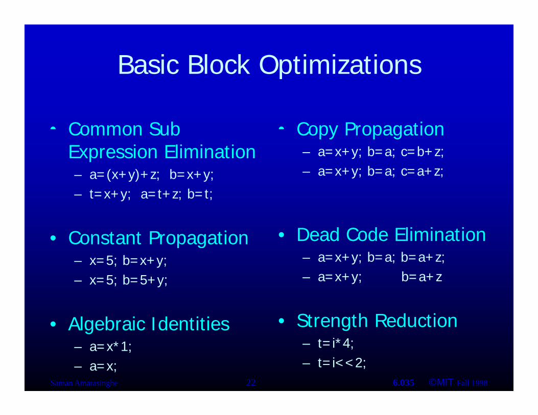
Basic Block Optimizationsp
• Common Sub- • Copy Propagation Common Sub Expression Elimination – a=(x+y)+z; b=x+y;
Copy Propagation – a=x+y; b=a; c=b+z; – a=x+y; b=a; c=a+z; ( y) y
– t=x+y; a=t+z; b=t;
Constant P opagation • Dead Code Elimination • Constant Propagation – x=5; b=x+y; – x=5; b=5+y;
• Dead Code Elimination – a=x+y; b=a; b=a+z; – a=x+y; b=a+z ; y;
• Algebraic Identities • Strength Reduction t i*4
Saman Amarasinghe 22 6.035 ©MIT Fall 1998
– a=x*1; – a=x;
– t=i*4; – t=i<<2;

Basic Block Analysis Approachy pp • Assume normalized basic block - all statements
are of the form – var = var op var (where op is a binary operator) – var = op var (where op is a unary operator) – var = var
• Simulate a symbolic execution of basic block – Reason about values of variables (or other
aspects of computation) – Derive property of interest
Saman Amarasinghe 23 6.035 ©MIT Fall 1998

odu d a a o u o a
Two Kinds of Variables
• Temporaries Introduced By Compilerp y p – Transfer values only within basic block – Introduced as part of instruction flatteningp g – Introduced by optimizations/transformations – Typically assigned to only onceTypically assigned to only once
• Program Variables Declared in original program– Declared in original program
– May be assigned to multiple times M t f l b t b i bl k
Saman Amarasinghe 24 6.035 ©MIT Fall 1998
– May transfer values between basic blocks

ead Code at o
Outline
• IntroductionIntroduction
• Basic Blocks
• Common Subexpression Elimination
C P ti • Copy Propagation
• Dead Code Elimination
• Algebraic Simplification
• Summary

Simulate execution of basic block
Value Numbering • Reason about values of variables and expressions
in the program – Simulate execution of basic block – Assign virtual value to each variable and expression
• Discovered property: which variables and expressions Discovered property: which variables and expressions have the same value
• SStanddardd use: – Common subexpression elimination – Typically combined with transformation thatTypically combined with transformation that
• Saves computed values in temporaries • Replaces expressions with temporaries when value
off expressiion previiouslly computtedd
Saman Amarasinghe 26 6.035 ©MIT Fall 1998
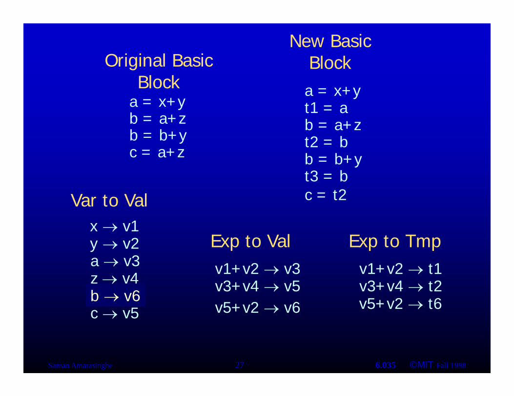
b v5
Original Basic New Basic
Block
a = x+y b = a+z
a = x+y t1 = a b = a+z
Block
b a z b = b+y c = a+z
b = a+z t2 = b b = b+y t3 bt3 = b
x v1
Var to Val c = t2
x v1 y v2 a v3
4 v1+v2 v3
Exp to Val v1+v2 t1
Exp to Tmp
b v6 z v4
c v5
v1+v2 v3 v3+v4 v5
v1+v2 t1 v3+v4 t2
v5+v2 v6 v5+v2 t6
Saman Amarasinghe 27 6.035 ©MIT Fall 1998

Value Numbering Summaryg y
• Forward symbolic execution of basic block
–
• Each new value assigned to temporary – a=x+y; becomes a=x+y; t=a;
Temporary preserves value for use later in program even Temporary preserves value for use later in program even if original variable rewritten • a=x+y; a=a+z; b=x+y becomes • a=x+y; t=a; a=a+z; b=t;
• Maps – V tVar to VVall – specifiifies symbbolilic vallue ffor eachh var iiablebl – Exp to Val – specifies value of each evaluated expression – Exp to Tmp – specifies tmp that holds value of each Exp to Tmp specifies tmp that holds value of each
evaluated expression
Saman Amarasinghe 28 6.035 ©MIT Fall 1998

=
•
Map Usagep g • Var to Val
– Used to compute symbolic value of y and z when f fprocessing statement of form x = y + z
• Exp to Tmpp p – Used to determine which tmp to use if value(y) +
value(z) previously computed when processing statement of form x = y + zstatement of form x y + z
• Exp to Val d d l h– Used to update Var to Val when
• processing statement of the form x = y + z, and • value(y) + value(z) previously computed
Saman Amarasinghe 29 6.035 ©MIT Fall 1998
value(y) + value(z) previously computed
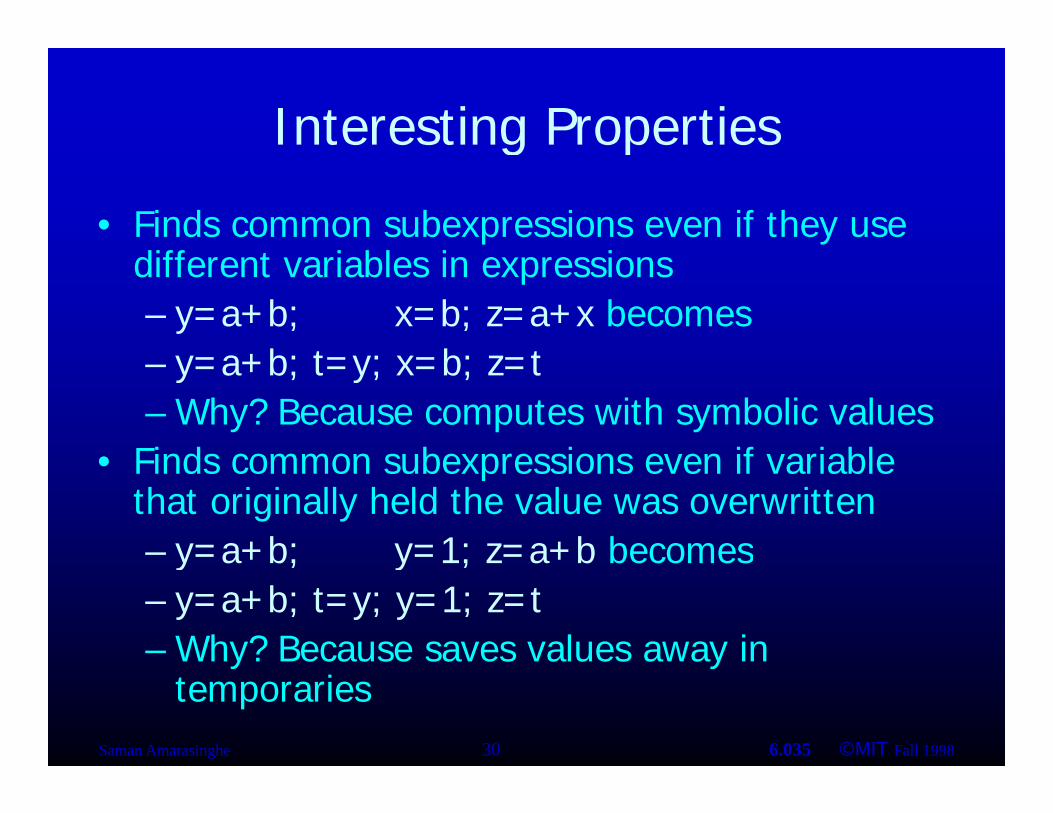
Interesting Propertiesg p
• Finds common subexpressions even if they use diff t i bl i idifferent variables in expressions – y=a+b; x=b; z=a+x becomes
y a+b; t y; x b; z t– y=a+b; t=y; x=b; z=t – Why? Because computes with symbolic values
• Finds common subexpressions even if variable • Finds common subexpressions even if variable that originally held the value was overwritten – y=a+b; y=1; z=a+b becomesy a+b; y 1; z a+b becomes – y=a+b; t=y; y=1; z=t – Why? Because saves values away in
Saman Amarasinghe 30 6.035 ©MIT Fall 1998
y y temporaries
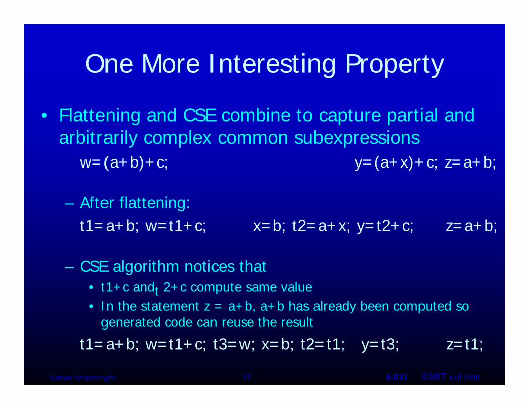
One More Interesting Propertyg p y
• Flattening and CSE combine to capture partial and arbitrarily complex common subexpressions
w=(a+b)+c;
x=b;
y=(a+x)+c; z=a+b;
– After flattening: a+b; w t1+c; a+x; y t2+c; z=a+b;t1t1=a+b; w=t1+c; xx b; =b; t2t2=a+x; y=t2+c; z a+b;
– CSE algorithm notices that • t11+c andd t 22+c compute same vallue • In the statement z = a+b, a+b has already been computed so
generated code can reuse the result
t1=a+b; w=t1+c; t3=w; x=b; t2=t1; y=t3; z=t1;
Saman Amarasinghe 31 6.035 ©MIT Fall 1998
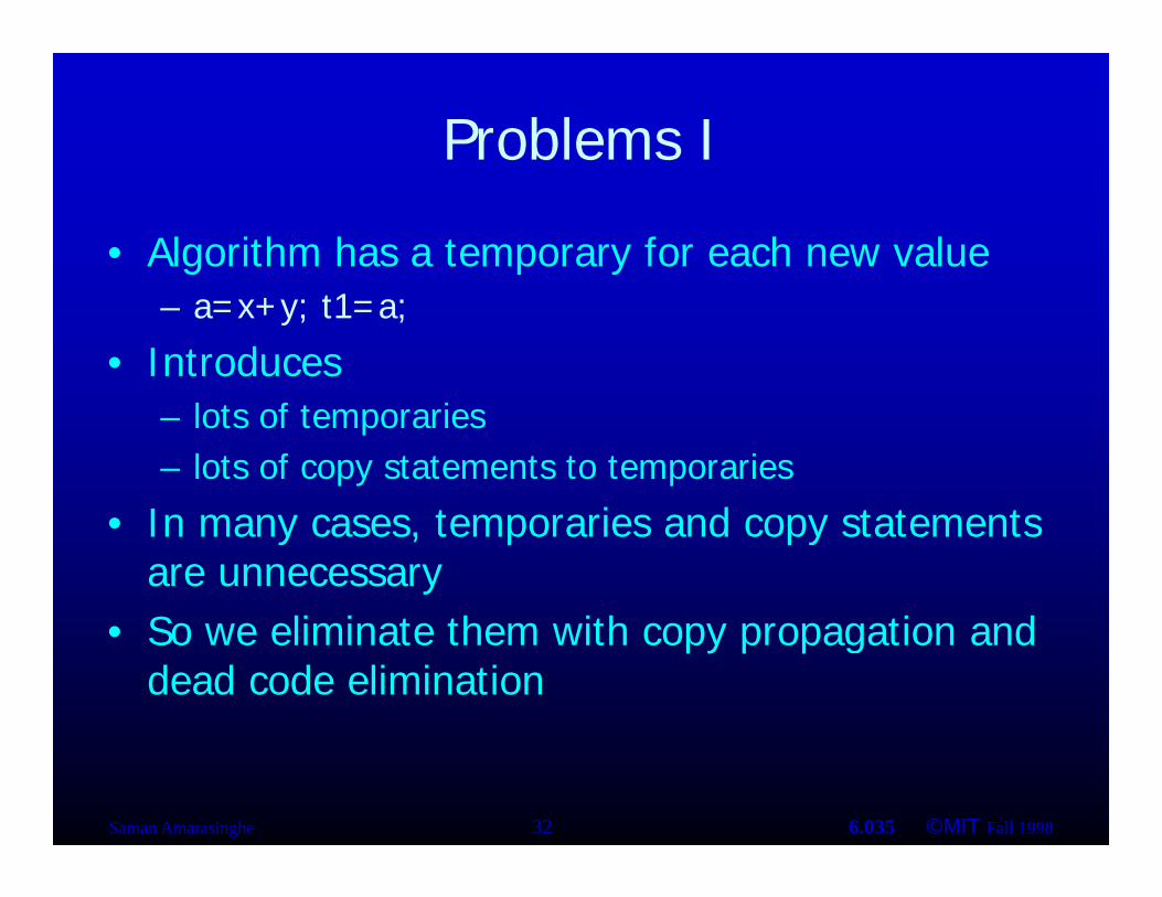
Problems I
• Algorithm has a temporary for each new value – a=x+y; t1=a;
• Introduces – lots of temporaries – lots of copy statements to temporaries
• In many cases, temporaries and copy statements are unnecessary S li i t th ith ti d• So we eliminate them with copy propagation and dead code elimination
Saman Amarasinghe 32 6.035 ©MIT Fall 1998

Problems II
• Expressions have to be identical – a=x+y+z; b=y+z+x; c=x*2+y+2*z–(x+z)
• We use canonicalization • We use algebraic simplification
Saman Amarasinghe 33 6.035 ©MIT Fall 1998
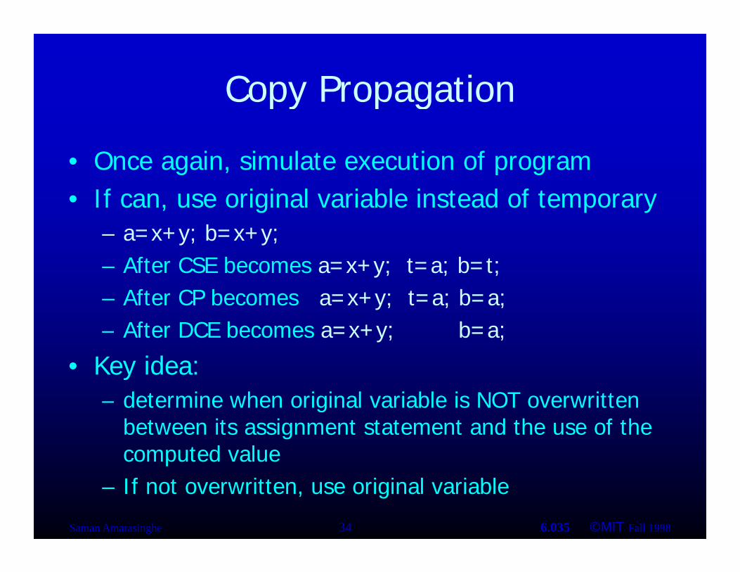
Copy Propagationpy p g
• Once again, simulate execution of program • If can, use original variable instead of temporary
– a=x+y; b=x+y; – After CSE becomes a=x+y; t=a; b=t; – After CP becomes a=x+y; t=a; b=a;
Aft DCE b b=a;– After DCE becomes a=x+y; b
• Key idea: d t i h i i l i bl i NOT itt– determine when original variable is NOT overwritten between its assignment statement and the use of the computed value
– If not overwritten, use original variable
Saman Amarasinghe 34 6.035 ©MIT Fall 1998

ead Code at o
Outline
• IntroductionIntroduction
• Basic Blocks
• Common Subexpression Elimination
C P ti • Copy Propagation
• Dead Code Elimination
• Algebraic Simplification
• Summary

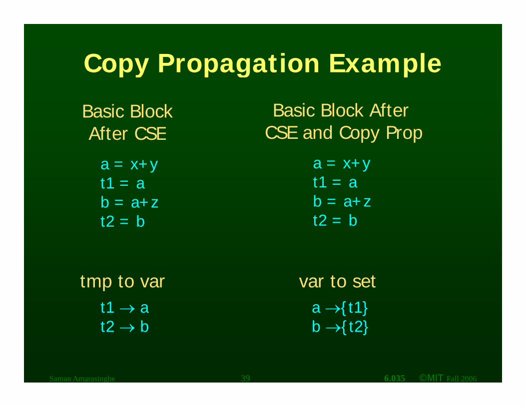
Copy Propagation Mapspy p g p
• Maintain two mapsp– tmp to var: tells which variable to use instead
of a given temporary variable – var to set: inverse of tmp to var. tells which
temps are mapped to a given variable by tmp to var
Saman Amarasinghe 36 6.035 ©MIT Fall 1998
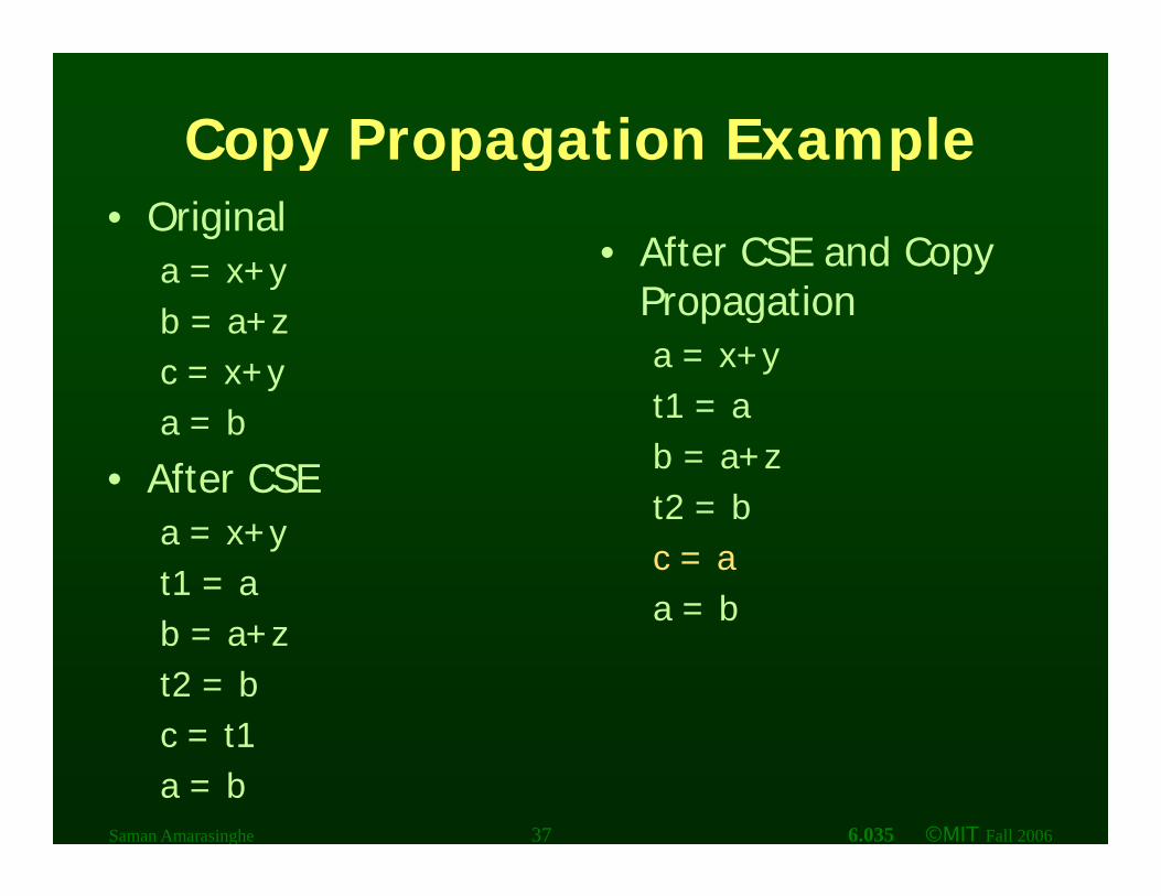
Copy Propagation Examplepy p g p • Original
• After CSE and Copy a = x+ya x+y
b = a+z Propagation
c = x+y a = x+y
a = b t1 = a
• After CSE b = a+z t2 = b t2 = b
a = x+y c = a
t1 = a a = bb
b = a+z a
t2 = b
c t1 c = t1
a = bSaman Amarasinghe 37 6.035 ©MIT Fall 2006

Copy Propagation Examplepy p g p
Basic Block Basic Block After Aft CSE CSECSE and C d Copy PProp After CSE
a = x+y a = x+yt1t1 = a t1t1 = a
tmp to var tmp to var var to set var to set t1 a a {t1}
Saman Amarasinghe 38 6.035 ©MIT Fall 2006
Copy Propagation Examplepy p g p
Basic Block Basic Block After Af CSE CSECSE and C d Copy PProp After CSE
a = x+y a = x+yt1t1 = a t1t1 = a b = a+z b = a+z t2 = b t2 = b
tmp to var tmp to var var to set var to set t1 a a {t1}t2 b bb {{t2}t2}t2 b
Saman Amarasinghe 39 6.035 ©MIT Fall 2006

Copy Propagation Examplepy p g p
Basic Block Basic Block After Aft CSE CSECSE and C d Copy PProp After CSE
a = x+y a = x+yt1t1 = a t1t1 = a b = a+z b = a+z t2 = b t2 = b c = t1
tmp to var tmp to var var to set var to set t1 a a {t1}t2 b bb {{t2}t2}t2 b
Saman Amarasinghe 40 6.035 ©MIT Fall 2006
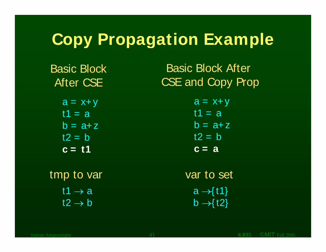
Copy Propagation Examplepy p g p
Basic Block Basic Block After Aft CSE CSECSE and C d Copy PProp After CSE
a = x+y a = x+yt1t1 = a t1t1 = a b = a+z b = a+z t2 = b t2 = b c = t1 c = a
tmp to var tmp to var var to set var to set t1 a a {t1}t2 b bb {{t2}t2}t2 b
Saman Amarasinghe 41 6.035 ©MIT Fall 2006

Copy Propagation Examplepy p g p
Basic Block Basic Block After Aft CSE CSECSE and C d Copy PProp After CSE
a = x+y a = x+yt1t1 = a t1t1 = a b = a+z b = a+z t2 = b t2 = b c = t1 c = a a = b a = b
tmp to var tmp to var var to set var to set t1 a a {t1}t2 b bb {{t2}t2}t2 b
Saman Amarasinghe 42 6.035 ©MIT Fall 2006

Copy Propagation Examplepy p g p
Basic Block Basic Block After Aft CSE CSECSE and C d Copy PProp After CSE
a = x+y a = x+yt1t1 = a t1t1 = a b = a+z b = a+z t2 = b t2 = b c = t1 c = a a = b a = b
tmp to var tmp to var var to set var to set t1 t1 a {}t2 b bb {{t2}t2}t2 b
Saman Amarasinghe 43 6.035 ©MIT Fall 2006

ead Code at o
Outline
• IntroductionIntroduction
• Basic Blocks
• Common Subexpression Elimination
C P ti • Copy Propagation
• Dead Code Elimination
• Algebraic Simplification
• Summary

•
=
Dead Code Elimination
• Copy propagation keeps all temps aroundpy p p g p p • May be temps that are never read • Dead Code Elimination removes themDead Code Elimination removes them
Basic Block After CSE and CP
Basic Block After CSE CP and DCE
a = x+y t1 = a
a = x+y b = a+z
CSE and CP CSE, CP and DCE
t1 a b = a+z t2 = b c = a
b a+z c = a a = b
Saman Amarasinghe 45 6.035 ©MIT Fall 1998
c = a a = b

a a a o a ab a a d d
Dead Code Elimination
• Basic Idea – Process Code In Reverse Execution Order – Maintain a set of variables that are needed
later in computation – If encounter an assignment to a temporaryg p y
that is not needed, remove assignment
Saman Amarasinghe 46 6.035 ©MIT Fall 1998

Basic Block After
a = x+y t1
CSE and Copy Prop
t1 = a b = a+z t2 = b c = a a = b
Needed Set {b}{ }
Saman Amarasinghe 47 6.035 ©MIT Fall 2006

Basic Block After
a = x+y t1
CSE and Copy Prop
t1 = a b = a+z t2 = b c = a a = b
Needed Set {a, b}{ , }
Saman Amarasinghe 48 6.035 ©MIT Fall 2006

Basic Block After
a = x+y t1
CSE and Copy Prop
t1 = a b = a+z t2 = b c = a a = b
Needed Set {a, b}{ , }
Saman Amarasinghe 49 6.035 ©MIT Fall 2006
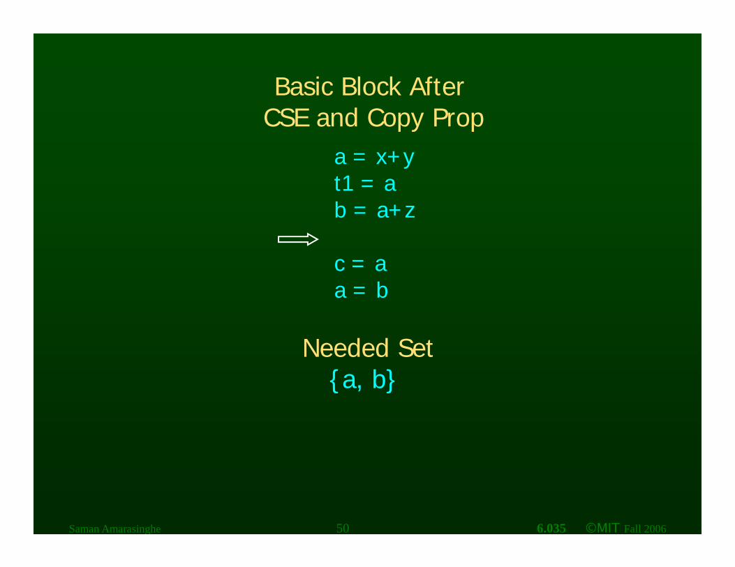
Basic Block After
a = x+y t1
CSE and Copy Prop
t1 = a b = a+z
c = a a = b
Needed Set {a, b}{ , }
Saman Amarasinghe 50 6.035 ©MIT Fall 2006

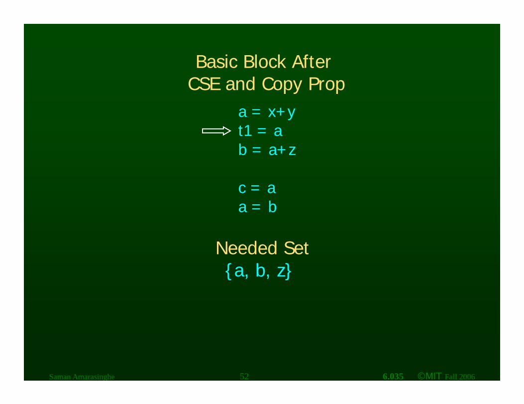
Basic Block After
a = x+y t1
CSE and Copy Prop
t1 = a b = a+z
c = a a = b
Needed Set {a, b, z}{ , , }
Saman Amarasinghe 51 6.035 ©MIT Fall 2006
Basic Block After
a = x+y t1
CSE and Copy Prop
t1 = a b = a+z
c = a a = b
Needed Set {a, b, z}{ , , }
Saman Amarasinghe 52 6.035 ©MIT Fall 2006

Basic Block After
a = x+y
CSE and Copy Prop
b = a+z
c = a a = b
Needed Set {a, b, z}{ , , }
Saman Amarasinghe 53 6.035 ©MIT Fall 2006
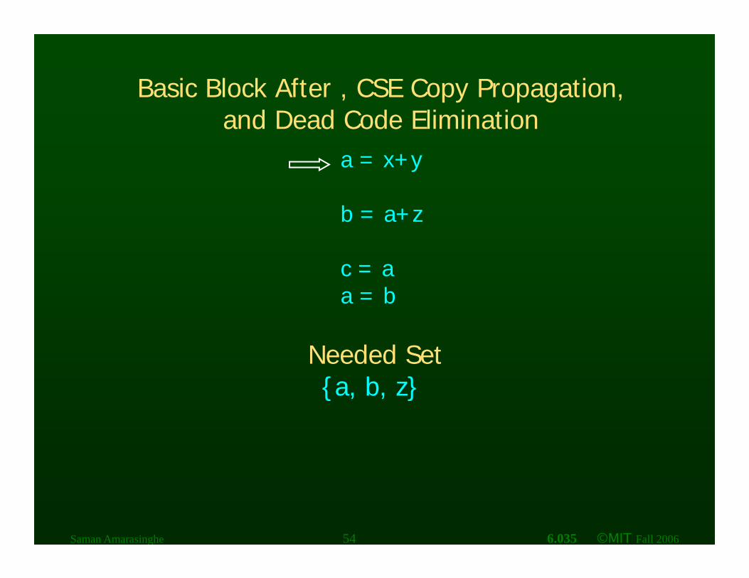
Basic Block After , CSE Copy Propagation,
a = x+y
and Dead Code Elimination
b = a+z
c = a a = b
Needed Set {a, b, z}{ , , }
Saman Amarasinghe 54 6.035 ©MIT Fall 2006

Basic Block After , CSE Copy Propagation, and Dead Code Elimination
a = x+y
b = a+z
c = a a = b
Needed Set{a, b, z}} { , ,
Saman Amarasinghe 55 6.035 ©MIT Fall 2006

ead Code at o
Outline
• IntroductionIntroduction
• Basic Blocks
• Common Subexpression Elimination
C P ti • Copy Propagation
• Dead Code Elimination
• Algebraic Simplification
• Summary

,
Algebraic Simplificationg p
• Applyy our knowledge from alggebra, numberpp gtheory etc. to simplify expressions
Saman Amarasinghe 57 6.035 ©MIT Fall 1998

,
Algebraic Simplificationg p
• Apply our knowledge from algebra, numberpp y g g theory etc. to simplify expressions
• ExampleExample – a + 0 a – a * 1 a – a / 1 a – a * 0 0
0– 0 - a -a – a + (-b) a - b – -(-a) a
Saman Amarasinghe 58 6.035 ©MIT Fall 1998
( a) a

,
Algebraic Simplificationg p
• Applyy our knowledge from alggebra, numberpp gtheory etc. to simplify expressions
• ExampleExample– a true a– a false false– a true true– a false a
Saman Amarasinghe 59 6.035 ©MIT Fall 1998
,
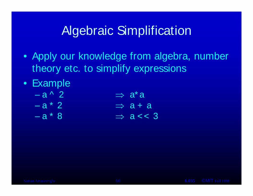
Algebraic Simplificationg p
• Applyy our knowledge from alggebra, numberpp gtheory etc. to simplify expressions
• ExampleExample– a ^ 2 a*a– a * 2 a + a – a * 8 a << 3
Saman Amarasinghe 60 6.035 ©MIT Fall 1998

•
Opportunities for Algebraic Simplification
• After compiler expansion
Programs are more readable with full expressions– Programmers are lazy to simplify expressions
In the code
Algebraic Simplification
• In the code
– Programs are more readable with full expressions
– Example: Array read A[8][12] will get expanded to
– *(Abase + 4*(12 + 8*256)) which can be simplified
• After other optimizations
Saman Amarasinghe 61 6.035 ©MIT Fall 1998

Usefulness of Algebraic Simplificationg p
R d th b f i t ti • Reduces the number of instructions • Uses less expensive instructions • Enable other optimizations
Saman Amarasinghe 62 6.035 ©MIT Fall 1998

•
Implementationp
• Not a data-flow optimization!p• Find candidates that matches the
simplification rules and simplify thesimplification rules and simplify the expression trees
• Candidates may not be obviousCandidates may not be obvious
Saman Amarasinghe 63 6.035 ©MIT Fall 1998

•
Implementationp
• Not a data-flow optimization!p• Find candidates that matches the
simplification rules and simplify thesimplification rules and simplify the expression trees
• Candidates may not be obviousCandidates may not be obvious – Example
a + b - a +
a + b a a -
Saman Amarasinghe 64 6.035 ©MIT Fall 1998
b a

•
Use knowledge about operatorsg p
• Commutative operatorsCommutative operators – a op b = b op a–
• Associative operators – ((a opp b)) opp c = b opp ((a opp c))
Saman Amarasinghe 65 6.035 ©MIT Fall 1998

Canonical Format
• Put expression trees into a canonical pformat – Sum of multiplicandsp– Variables/terms in a canonical order – ExampleExample
(a+3)*(a+8)*4 4*a*a+44*a+96
– Section 12.3.1 of whale book talks about this
Saman Amarasinghe 66 6.035 ©MIT Fall 1998

Effects on the Numerical Stabilityy
• Some alggebraic simpplifications mayy p produce incorrect results
Saman Amarasinghe 67 6.035 ©MIT Fall 1998
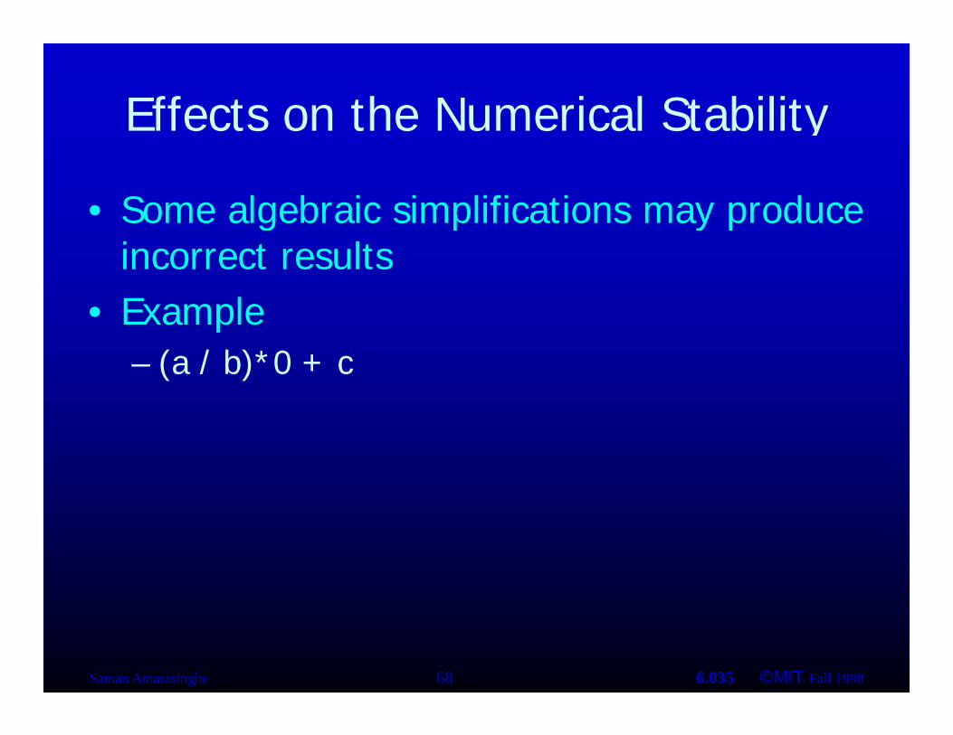
Effects on the Numerical Stabilityy
• Some alggebraic simpplifications mayy p produce incorrect results
• ExampleExample – (a / b)*0 + c
Saman Amarasinghe 68 6.035 ©MIT Fall 1998
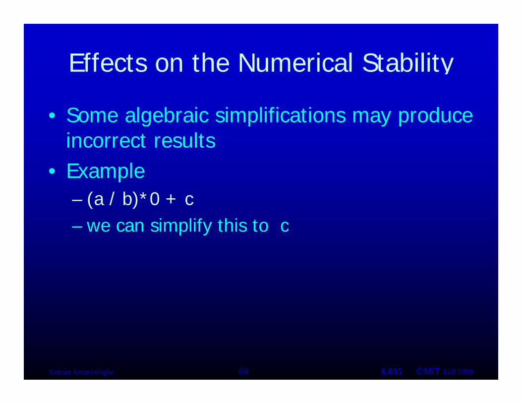
Effects on the Numerical Stabilityy
• Some alggebraic simpplifications mayy p produce incorrect results
• ExampleExample – (a / b)*0 + c – we can simplify this to we can simplify this to cc
Saman Amarasinghe 69 6.035 ©MIT Fall 1998
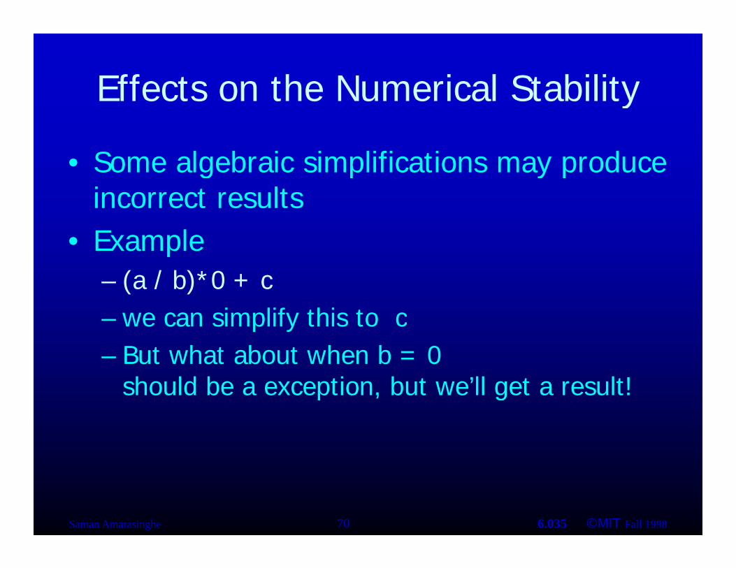
Effects on the Numerical Stabilityy
• Some alggebraic simpplifications mayy p produce incorrect results
• ExampleExample – (a / b)*0 + c – we can simplify this to we can simplify this to cc – But what about when b = 0
should be a exception, but we’ll get a result! should be a exception, but we ll get a result!
Saman Amarasinghe 70 6.035 ©MIT Fall 1998

ead Code at o
Outline
• IntroductionIntroduction
• Basic Blocks
• Common Subexpression Elimination
C P ti • Copy Propagation
• Dead Code Elimination
• Algebraic Simplification
• Summary

Interesting Propertiesg p
• Analysis and Transformation Algorithms S b li ll Si l t E ti f PSymbolically Simulate Execution of Program – CSE and Copy Propagation go forward – Dead Code Elimination goes backwardsDead Code Elimination goes backwards
• Transformations stacked – Group of basic transformations work together – Often, one transformation creates inefficient code that
is cleaned up by following transformationsis cleaned up by following transformations – Transformations can be useful even if original code
may not benefit from transformation
Saman Amarasinghe 72 6.035 ©MIT Fall 1998

= =
Other Basic Block Transformations
• Constant Propagationp g• Strength Reduction
– a<<2 = a*4; a+a+a = 3*a;a<<2 a 4; a+a+a 3 a;
• Do these in unified transformation framework not in earlier or later phases framework, not in earlier or later phases
Saman Amarasinghe 73 6.035 ©MIT Fall 1998

t t
Summaryy
• Basic block analyses and transformations • SSymbbolilicalllly siimullate executiion off program
– Forward (CSE, copy prop, constant prop) – Backward (Dead code elimination)
• Stacked groups of analyses and transformations that work together – CSE introduces excess tempporaries and copypy statements – Copy propagation often eliminates need to keep temporary
variables around – Dead code elimination removes useless code
• Similar in spirit to many analyses and transformations that operate across basic blocks
Saman Amarasinghe 74 6.035 ©MIT Fall 1998
MIT OpenCourseWarehttp://ocw.mit.edu
6.035 Computer Language Engineering Spring 2010
For information about citing these materials or our Terms of Use, visit: http://ocw.mit.edu/terms.


