30
Lecture Notes in Mathematics Editors: A. Dold, Heidelberg E Takens, Groningen 1665
| Date post: | 18-May-2018 |
| Category: |
Documents |
| Upload: | nguyentruc |
| View: | 216 times |
| Download: | 1 times |
Lecture Notes in Mathematics Editors: A. Dold, Heidelberg E Takens, Groningen
1665

Springer Berlin Heidelberg New York Barcelona Budapest Hong Kong London Milan Paris Santa Clara Singapore Tokyo

E. Gin6 G.R. Grimmett L. Saloff-Coste
Lectures on Probability Theory and Statistics
Ecole d 'Et6 de Probabilit6s
de Saint-Flour XXVI - 1996
Editor: R Bernard
Springer

Authors
Evarist Gin6 Department of Mathematics University of Connecticut 196 Auditorium Road (U-9, R. 111) Storrs, CT 06269-3009, USA
Geoffrey R. Grimmett Statistical Laboratory University of Cambridge 16 Mill Lane Cambridge, CB2 1SB, UK
Laurent Saloff-Coste Laboratoire de Statistique et Probabilites Universit6 Paul Sabatier 118, Route de Narbonne F-31062 Toulouse, France
Editor
Pierre Bernard Laboratoire de Math6matiques Appliqu6es UMR CNRS 6620 Universit6 Blaise Pascal Clermont-Ferrand F-63177 Aubi6re, France
Cataloging-in-Publication Data applied for
Die Deutsche Bibliothek - CIP-Einheitsaufnahme
Lectures on probability theory and statistics / Ecole d'Et6 de Probabilitds de Saint-Flour XXVI - 1996. E. Gin6 ... Ed.: E Bernard. - Berlin; Heidelberg; New York; Barcelona; Budapest; Hong Kong; London; Milan; Paris; Santa Clara; Singapore; Tokyo: Springer, 1997 (Lecture notes in mathematics; Vol. 1665) ISBN 3-540-63190-9
Mathematics Subject Classification (1991): 46N30, 47D07, 60-01, 60-06, 60B12, 60F15, 60G50, 60G60, 60J25, 60J27, 60K35, 62-01, 62-02, 62-06, 62G05
ISSN 0075- 8434 ISBN 3-540-63190-9 Springer-Verlag Berlin Heidelberg New York
This work is subject to copyright. All rights are reserved, whether the whole or part of the material is concerned, specifically the rights of translation, reprinting, re-use of illustrations, recitation, broadcasting, reproduction on microfilms or in any other way, and storage in data banks. Duplication of this publication or parts thereof is permitted only under the provisions of the German Copyright Law of September 9, 1965, in its current version, and permission for use must always be obtained from Springer-Verlag. Violations are liable for prosecution under the German Copyright Law.
�9 Springer-Verlag Berlin Heidelberg 1997 Printed in Germany
The use of general descriptive names, registered names, trademarks, etc. in this publication does not imply, even in the absence of a specific statement, that such names are exempt from the relevant protective laws and regulations and therefore free for general use.
Typesetting: Camera-ready TEX output by the authors SPIN: 10553291 46/3142-543210 - Printed on acid-free paper

I N T R O D U C T I O N
This volume contains lectures g iven a t t he Sain t -Flour Summer School of P robab i l i ty Theory dur ing the period 19th A u g u s t - 4 th September , 1996.
We t h a n k the authors for all t h e h a r d work they accomplished. Their lectures are a work of reference in the i r domain.
The school brought toge ther 74 par t i c ipan t s , 38 of whom gave a lecture concerning the i r research work.
At the end of this volume you will f ind t he list of par t ic ipants and thei r papers.
Finally, to facilitate research conce rn ing previous schools we give here the n u m b e r of t h e volume of "Lecture Notes" where t hey can b e found :
L e c t u r e N o t e s in M a t h e m a t i c s
1971: n ~ 1 9 7 3 : n ~ - 1 9 7 7 : n ~ - 1 9 7 8 : n ~ - 1982: n ~ 1983: n ~ 1988 : n ~ 1989: n~ 1993 : n ~ 1 9 9 4 : n ~
1 9 7 4 : n ~ - 1975: n ~ 1 9 7 6 : n ~ - 1 9 7 9 : n ~ - 1980: n~ 1 9 8 1 : n ~ - 1984 : n~ - 1985 - 1986et 1 9 8 7 : n ~ - 1990 : n ~ 1991: n~ 1 9 9 2 : n ~
L e c t u r e N o t e s in S t a t i s t i c s
1986 : n~

TABLE OF CONTENTS
E v a r i s t G I N E : " D E C O U P L I N G A N D L I M I T T H E O R E M S F O R U - S T A T I S T I C S A N D U - P R O C E S S E S "
1. Introduction
2. Decoupling inequalities
3. Limit theorems for U-statistics
4. Limit theorems for U-processes
References
2
3
12
24
32
E v a r i s t G I N E : " L E C T U R E S O N S O M E A S P E C T S T H E O R Y O F T H E B O O T S T R A P "
Preface
1. On the bootstrap in ]R
1.1 Efron's bootstrap of the mean in ]R 1.2 The general exchangeable bootstrap of the mean 1.3 The bootstrap of the mean for stationary sequences 1.4 The bootstrap of U-statistics 1.5 A general m out of n bootstrap
37
39
41
41 54 59 64 76
2. On the bootstrap for empirical processes
2.1 Background from empirical process theory 2.2 Poissonization inequalities and Efron's bootstrap in probability 2.3 The almost sure Efron's bootstrap 2.4 The exchangeable bootstrap 2.5 Uniformly pregaussian classes of functions and the bootstrap 2.6 Some remarks on applications
83
83 103 113 119 128 139
References 147
viii
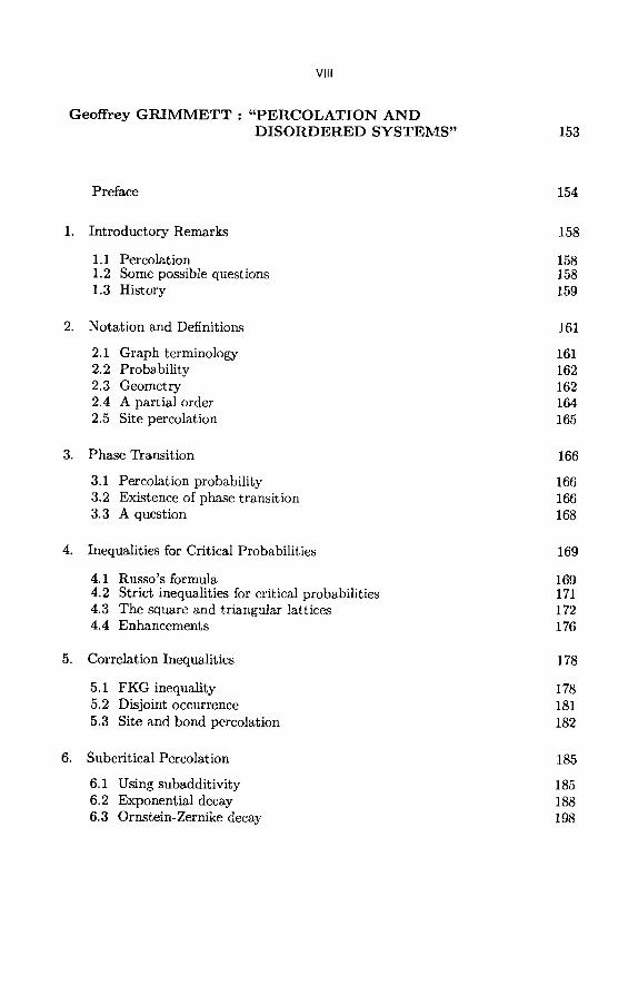
G e o f f r e y G R I M M E T T : " P E R C O L A T I O N A N D D I S O R D E R E D S Y S T E M S " 153
Preface
1. Introductory Remarks
1.1 Percolation 1.2 Some possible questions 1.3 History
2. Notation and Definitions
2.1 Graph terminology 2.2 Probability 2.3 Geometry 2.4 A partial order 2.5 Site percolation
3. Phase Transition
3.1 Percolation probability 3.2 Existence of phase transition 3.3 A question
4. Inequalities for Critical Probabilities
4.1 Russo's formula 4.2 Strict inequalities for critical probabilities 4.3 The square and triangular lattices 4.4 Enhancements
5. Correlation Inequalities
5.1 FKG inequality 5.2 Disjoint occurrence 5.3 Site and bond percolation
6. Subcritical Percolation
6.1 Using subadditivity 6.2 Exponential decay 6 .30rnste in-Zernike decay
154
158
158 158 159
161
161 162 162 164 165
166
166 166 168
169
169 171 172 176
178
178 181 182
185
185 188 198

IX
7. Supercritical Percolation
7.1 Uniqueness of the infinite cluster 7.2 Percolation in slabs 7.3 Limit of slab critical points 7.4 Percolation in half-spaces 7.5 Percolation probability 7.6 Cluster-size distribution
8. Critical Percolation
8.1 Percolation probability 8.2 Critical exponents 8.3 Scaling theory 8.4 Rigorous results 8.5 Mean-field theory
9. Percolation in Two Dimensions
9.1 The critical probability is 1/2 9.2 RSW technology 9.3 Conformal invariance
10. Random Walks in Random Labyrinths
10.1 Random walk on the infinite percolation cluster 10.2 Random walks in two-dimensional labyrinths 10.3 General labyrinths
11. Fractal Percolation
11.1 Random fractals 11.2 Percolation 11.3 A morphology 11.4 Relationship to Brownian Motion
12. Ising and Potts Models
12.1 Ising model for ferromagnets 12.2 Potts models 12.3 Random-cluster models
13. Random-Cluster Models
13.1 Basic properties 13.2 Weak limits and phase transitions 13.3 First and second order transitions 13.4 Exponential decay in the subcritical phase 13.5 The case of two dimensions
199
199 201 202 215 216 218
219
219 219 219 221 221
229
229 230 233
236
236 240 248
254
254 255 258 260
261
261 262 263
265
265 266 268 269 273
References 281
•
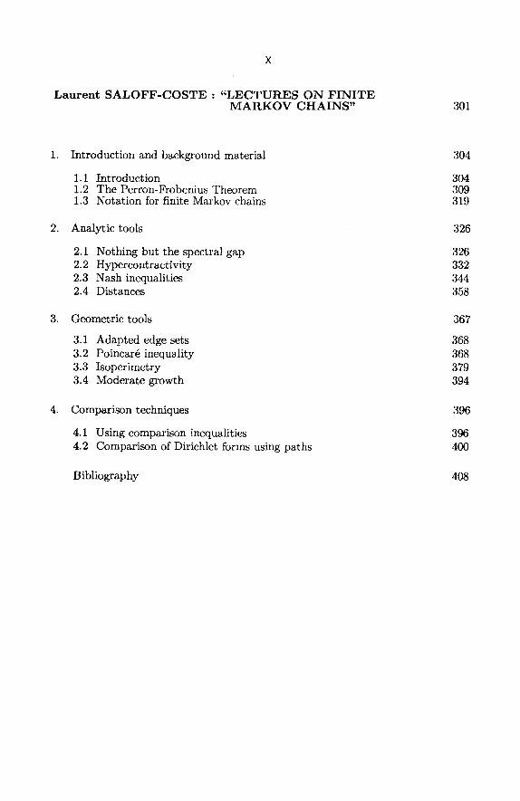
L a u r e n t S A L O F F - C O S T E : " L E C T U R E S O N F I N I T E M A R K O V C H A I N S " 301
1. Introduction and background material
1.1 Introduction 1.2 The Perron-Frobenius Theorem 1.3 Notation for finite Markov chains
2. Analytic tools
2.1 Nothing but the spectral gap 2.2 Hypercontractivity 2.3 Nash inequalities 2.4 Distances
3. Geometric tools
3.1 Adapted edge sets 3.2 Poincar~ inequality 3.3 Isoperimetry 3.4 Moderate growth
4. Comparison techniques
4.1 Using comparison inequalities 4.2 Comparison of Dirichlet forms using paths
304
304 309 319
326
326 332 344 358
367
368 368 379 394
396
396 40O
Bibliography 408
D E C O U P L I N G A N D L I M I T T H E O R E M S
F O R U-STATISTICS A N D U-PROCESSES
Evarist GINE (-)
(*) Work partially supported by NSF Crants Nos. DMS-9300725 and DMS-9625457 and by the CNHS through the Laboratoiro de Math~matiques Appliqu~es de l'Universit~ Blaise P~cal, Clermont-Ferrand, ~ranc6.

1. I n t r o d u c t i o n . Recently discovered decoupling inequalities for U-processes (mainly, de la Pefia, 1992, and de la Pefia and Montgomery-Smith, 1995) have had important consequences for the asymptotic theory of U statistics and U processes (Gin4 and Zinn, 1994, and Arcones and Gin6, 1993, 1995, among others). It is the object of these lectures to describe these developments.
U statistics, first considered by Halmos (1946) in connection with unbiased estimators and formally introduced by Hoeffding (1948), are defined as follows:
�9 oo given an i.i.d, sequence of random variables {X,}i=I with values in a measurable space (S,,5), and a measurable function h : S m --* R, the U statistics of order m and kernel h based on the sequence { X i } are
v . ( h ) - ('~ - ~)! .~, ( 1 . 1 ) h ( x i l , . . . , x i m ) , n >_ 72!
(il,...,im)cz~
w h e r e
I m = {((i l , . -- , i ra) : ij E N, 1 <_ ij < n, ij 7s ik if j 7~ k}.
These objects appear often in Statistics either as unbiased estimators of parameters of interest or, perhaps more often, as components of higher order terms in expan- sions of smooth statistics (yon Mises expansion, delta method). Particularly in connection with yon Mises expansions, it is sometimes convenient to also consider U-processes indexed by families 7-g of kernels, that is, collections of U-sta t i s t ics {U~(h) : h �9 ~}.
By a decoupling result for U statistics we mean a (usually two-sided) inequality between the quantities
E (I (1.2)
and (1.3)
IF
Xk possibly multiplied by constants that depend only on m, where the sequences { i }, k = 1 , . . . , m, axe independent copies of the original sequence {Xi}, and �9 is a non- negative function. Two quite different types of functions (~ have been considered:
convex (thus including ~(Ixl) -- Ixl p, p > 1) and ~(Ixl) = ~ , > , . The variables at the different coordinates of the domain of h in the deeoupled
statistic come from different independent sequences and therefore a decoupled U- statistic can be treated, conditionally on all but one of these sequences, as a sum of independent random variables. Clearly then, decoupling inequalities will allow for conditional use of Lfvy type maximal inequalities and for randomization by Rademaeher variables, which then turn U-statistics into Rademaeher chaos pro- cesses conditionally on the X samples. In this way, the analysis of U-processes can proceed more or less by analogy with that of empirical processes.
In Section 2 we describe the pertinent decoupling results and the randomization lemma. Section 3 is devoted to the central limit theorem and to the law of the iterated logarithm for U-statistics, and Section 4 to U-processes.

Contrary to the case of the boots t rap lectures in this volume, which are almost self-contained, here we present no technical details and refer the reader, instead, to the book 'An Introduction to Decoupling inequalities and Applications' by de la Pefia and myself, in preparation, or to the original articles.
I thank the organizers of, and the participants in, the Saint-Flour l~cole d'l~t@ de Calcul de Probabilit~s for the opportuni ty to present these lectures. I would like to mention here that both, these lectures and the boots t rap lectures in this volume have their origin in a short course on these same topics that I gave at the Universit@ de Paris-Sud (Orsay) in 1993. It is therefore a pleasure for me to also extend my grat i tude to the Orsay Statistics group.
2. D e c o u p l i n g inequa l i t i e s , a) Decoupling. Let ( S , S , P ) be a probability space. Consider collections ~il...im of measurable functions h : S m -+ R for ( i l , . . . , i m ) E I TM, with n > m (these functions can also be Banach space valued, but this would not actually change the level of generality of the results to be stated below). It is convenient to have the following definition: an envelope (or a mea- surable envelope) of a class of functions ~il...im is any measurable function Hil...im s u c h t h a t s u p h ~ ~ ~ I h ( x l , . . . , X m ) i < Hi l . . . i~ (X l , . . . ,Xm) for all x l , . . . , X m E S. All the classes of ~unctions considered here will have everywhere finite envelope.
Some s tandard notation: We set
I Ih(Xl , . . . ,Xm)ll, , := sup Ih(X~, . . . ,Xm)l h E T - /
for any collection of kernels 7-/, and we even write ]]hl] for ]]hi[~ if no confusion is possible. Since these are often uncountable suprema of random variables, they may not be measurable; in this case we write s and Pr* for outer expectation and probability (see the lecture notes on the bootstrap in this volume, chapter 2).
The main result about decoupling that we use in this article is the following theorem of de la Pefia (1992):
2.1. THEOREM. For natural numbers n > m, let X , , X i k, i = 1 , . . . ,n, k = 1 , . . . , rn, be the coordinate functions of the product probability space (S '~(m+l), S n(m+l), (P~ x . . . x Pn) re+l), in particular the variables { X { } ~ are in- dependent S valued random variables, Xi with probability iaw Pi, i <_ n, and
X ~ the sequences I xk l '~ 1r < rn, are i.i.d, copies of the sequence { i}{=1 For t i J i = l ~ - -
each ( i l , . . . ,ira) E ~ , let 7-til...im be a collection of measurable functions hi~...im : S m ---+ R admit t ing an everywhere finite measurable envelope Hi,...i~ such that ~ .Hi~ . . . im(X1, . . . ,X=) < oo. Let r : [0, oo) --, [0,0o) be a convex non decreasing function such that ,Xm)) < oo for a l / ( i l , . . . �9 Ir Then,
E*#2( sup I ~ h i l . . . i ~ ( X i ~ , . . . , X i , ~ ) [ ) hil...irn E'~it,. .ira I m
<E*g2(Cm sup I~ -~h i , . . . i . , (X : , , . . . ,X i=) 0 (2.1) h i l ' " im E"~il '" im I ~

where Cm = 2m(ra m - 1)((rn - 1) (m-l) - 1) • . . . • 3. If, moreover, the classes ~it...im satisfy that for all hil...im E 7-fil ...ira, z l , �9 �9 Zm E S and permutations s of {1,...,~},
hi,...~,o(Xl,... , x m ) : h,,,.. ~,~ (x , , , . . . ,x~m), (2.2) then
E*r 2(2m_2 r a - 1 ) ! h q ; m e ' u q . ~ Ig' . . . . " ' " 'm
_< E * * ( sup 1~-~ hi~ . . . im(Zi~ , ' " ,X i , , ) [ ) " (2.3) \hil., ,im E']'~il. im I~
For the proof of this theorem we refer to the above mentioned article of de la Pefia or to our forthcoming book. However, we indicate here the proof of Theorem 1.2 for m = 2 and 7-{~ = 7-f for M1 {i~, i2}, countable. In this proof, I1-It win denote the sup over h E 7-{.
PROOF OF THEOREM 2.1 under the stated restrictions. We replace X/1, X~ respec- tively by Xi , X~. Let {ei}i'~l be independent random variables uniformly distributed
I n on a set with two elements, say { - 1 , 1}, independent of {X~,Xi}~=I, and let Z~ and Z~, i = 1 , . . . n, be defined as follows:
Zi = { X i i f e i = l , { X: i f r (2.4) X~ if r = - 1 ' Z i = Xi if Ci = - - 1 '
If, for each 1 < i < n, P/ is the law of Xi then the law of the vector ( Z 1 , . . . , Z , , Z ~ , . . . , Z ' ) is (P1 x .- . x Pn) 2 since for each fixed e l , . . . , e,~ the coordinates of this vector are just 2n independent variables such that Pi is the law of the i-th and the (n + i)-th, i = 1 , . . . , n . That is,
C(Zl,. z , , z ; , z ' ) ~(x~,. . ' x ' ) . �9 ., . . . , = . , X n , X 1 , . . . ,
Likewise, s ,Z,~) = C(X1, . - . ,X,,). Therefore, for any (P1 x - . . • Pn) 2- integrable functions f and (P1 • "'" x P,~)-integrable functions g we have
Ef ( Z 1 , . . . , Z , , , Z ~ , . . . , Z ~ ) = Ef(X~,...,X,~,X2,...; Xn) , '
E g ( Z l , . . . , Zn) : I I~g (X l , . . . , X n ) . ( 2 . 5 )
Note also that , if Z is the a-a lgebra generated by the X variables,
Z = a ( X i , X ~ : i = 1 , . . . , n ) ,
then conditional integration with respect to Z of any function of the Z variables is simply integration with respect to the r variables only. In particular, for all i r j ,
E(h(Z~, Z j ) lZ ) = E(h(Zi, Z])l z ) = E(h(Z;, &) l z ) = ~,(h(Z~, Z})I z )
:

These observations i.e., equations (2.5) and (2.6), together with the convexity and monotonieity of O, the integrability of the functions involved, and Jensen's inequal- ity, justify the following two strings of inequalities which, together, prove the theo- rem. 1) For h symmetric in its entries,
E(I, (I I ~ h(Xi, X~)ll) = E~(~ II Y~ h(X~, X~) + ~. h(Xg, Xj)ll)
_< �89 [h(x. x~)+ h(x:,xj)+ h(x~,xj)+ h(x:,x~)] II) z~
Jr- } ~(211E h(Xi'Xj)H) q- 1E(I)(2H Z h(X:' X~ )11)
-- 1Eq'(4ll ~ G(h(Z,, Zr ~-E~(211 ~ h(x,, x~)ll)
-< E e ( 411Z h ( X i ' X j ) l l ) ' (2.7) z~
proving (2.3). Note that symmetry is essential for the first identity. 2) For h not necessarily symmetric, letting X = (7(Xi : i = 1 , . . . , n) , we have
EO(I I ~ h ( X i , Xj)ll )
_< ~ (211 y~E[h(X.Xj) + h(X:,Xj) + h(X.X}) + h(X:,X$)lx]ll)
< ~a~(2, E[h(x,,~,)+ ~(<,~,)+ a(~,,x;)+ ~(<, x~)3 II)
+ ~o(611 ~ E(h(Xf,X})IX)II)
<_ ~a~(sll EE(h(z,,z/z)ll) + ~-E~(6, E h(x,,x~),)
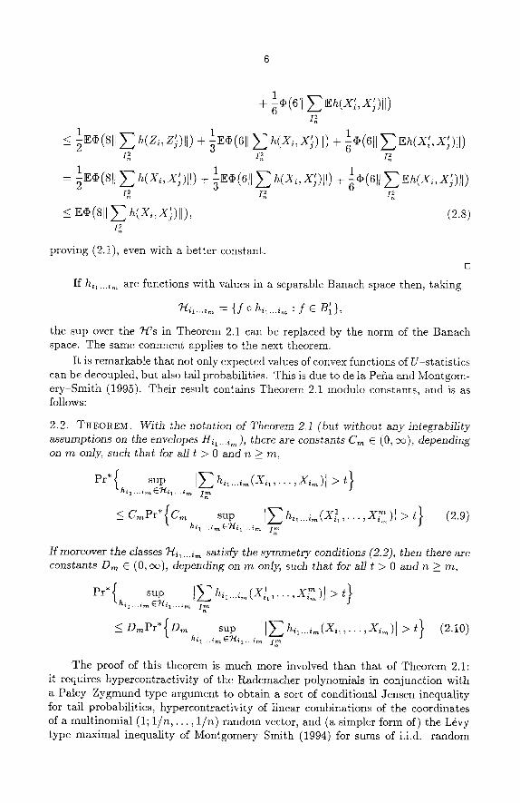
+ 6~(611 ~: Eh(X;, X~)ll)
_< Ee(811 y ~ h(Xi ,X j ) l l ) , (2.8) r~
proving (2.1), even with a better constant. []
If h 6...i~ are functions with values in a separable Banach space then, taking
"]-{il...i~ = { f o hil...im : f E B~ },
the sup over the 7-/'s in Theorem 2.1 can be replaced by the norm of the Banach space. The same comment applies to tile next theorem.
It is remarkable that not only expected values of convex functions of U-statistics can be decoupled, but also tail probabilities. This is due to de la Pefia and Montgom- ery-Smith (1995). Their result contains Theorem 2.1 modulo constants, and is as follows:
2.2. THEOREM. With the notation of Theorem 2.1 (but without any integrability assumptions on the envelopes H6...i~), there are constants Cm E (0, oo), depending on m only, such that for all t > 0 and n >_ m,
Pr*{ sup I E h i ~ . . . i ~ ( X i , , . . . , X i ~ ) l > t } hi l ' " im ~ i l ' " i m I ~
< C m P r * { C m sup I E h i , x , x ~ } . . . . ~ ( i , , . . - , ~ ) f >~ (z9) hq.. ~ ET/q...i,~ I F
/s the classes ~il...im satisfy the symmetry conditions (2.2), then there are constants Dm 6 (0, ~ ) , depending on m only, such that for aJl t > 0 and n >_ m,
Pr*( sup ,m(x t , . . , x TM~,,,)J ~ hq -im E~Q1..-im I F
< DmPr*{Dm sup > hl i ..im ~ i l . . . i m I F
The proof of this theorem is much more involved than that of Theorem 2.1: it requires hypercontractivity of the Rademacher polynomials in conjunction with a Paley Zygmund type argument to obtain a sort of conditional Jensen inequality for tail probabilities, hypercontractivity of linear combinations of the coordinates of a multinomial (1; 1 / n , . . . , 1/n) random vector, and (a simpler form of) the L6vy type maximal inequality of Montgomery Smith (1994) for sums of i.i.d, random
vectors. See de la Pefia and Montgomery Smith (1995) or our forthcoming book for the proof.
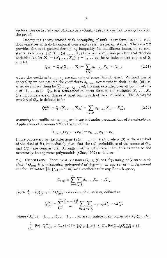
Decoupling theory started with deeoupling of multilinear forms in i.i.d, ran- dom variables with distributional constraints (e.g., Gaussian, stable). Theorem 2.2 provides the most general decoupling inequality for multilinear forms, up to con- stants, as follows. Let X = ( X 1 , . . . , Xn) be a vector of n independent real random variables Xi, let Xj = (X~ , . . . ,X~), j = 1 , . . . ,m, be m independent copies of X and let
Qm := Q m ( X , . . . , x ) = ~ a~l. . .~J~ 1 . . . x ~ , ( z l l ) iEs~-"
where the coefficients ail...im are elements of some Banach space. Without loss of generality we can assume the coefficients ail...im symmetric in their entries (other- wise, we replace them by y~ ai~o)...i,(m )/m!, the sum extended over all permutat ions s of { 1 , . . . , m } ) . Q,~ is a tetrahedral m-linear form in the variables X ~ , . . . , X ~ (its monomials are of degree at most one in each of these variables). The decoupled version of Qm is defined to be
Qa~r ~ X 1 .. Xm rn := Q n ( X l , . . . , X m ) �9 (2.12) ail , . . im il zm ~ iEz;, ~
assuming the coefficients ai~...i~ are invariant under permutations of its subindices. Application of Theorem 2.2 to the functions
h i l . . . i , ~ ( X l , . . . , X r n ) = a i , . . . imXi i " ' ' X i ~
(more concretely to the collections { f (h i~ . . . i~) : f E B~}, where B[ is the unit ball of the dual of B), immediately gives that the tail probabilities of the norms of Qm and Qd~ are comparable. Actually, with a little extra care, this extends to not necessarily homogenous polynomials (Gin6, 1997) as follows:
2.3. COROLLARY. There exist constants Cm E (0, ec) depending only on m such that if Q(~) is a tetrahedral polynomied of degree m in any set of n independent random variables {Xi}in__l , n > m , with coet~cients in any Banach space,
Q(m) = ~ E a i l . . . i k X i ~ ' " X i k k=O iEI~
(with _To = {0}), and i[ odec is its decoupled version, deigned as
= ,...., a~...~Xi~ "Xi~ , k=O iEI~ ~Ez~
where { X / : i = 1 , . . 3" = i , . . . , m , are m independent copies or then
1 a~c Cmt} < t} < Cm Pr{Cm er t}. Cm Pr{IiQ('~)II > _ Pr{IIQ(,~)II > _ IiQ(m)II >

This result should not be considered new since it is a trivial consequence of Theorem 2.2, but it is formally new in the sense that previously published versions of it require the variables Xi to be symmetric and the polynomials to be homogeneous (Kwapiefi and Woyczynski, 1992; de la Pefia, Montgomery-Smith and Szulga, 1994), or the variables to be symmetric and to have expected values of convex functions instead of tail probabilities in the inequalities (Kwapiefi, 1987).
Neither Theorem 2.2 nor Corollary 2.3 will be used in the sequel.
b) Randomizat ion of convex functions. What interests us about decoupling is the possibility of randomizing a degenerate U-process (or a degenerate U statistic). In order to be more concrete, we will have to define the degree of degeneracy of a U-stat is t ic and also recall Hoeffding's decomposition.
As usual, we let (S, $) be a measurable space and P a probability measure on
it, and let Xi, X} j) ci, cl j) be the coordinate functions on the product of countably many copies of (S, S, P) and countably many copies of ( { - 1 , 1}, ((~1 Jr- (~-1)/2). In particular these variables are all independent, the X ' s have law P, and the e's are Rademacher variables.
2.4. DEFINITION. A pm integrable symmetr ic function o f m variables, h : S m --* R, is P -degenerate of order r - 1, 1 < r <_ m, i f
/ h ( z l , . . . , x m ) d P m - r + l ( z ~ , . . . , x m ) = / h d P m for a l l z l , . . . , Z r _ l E S
whereas
h ( z l , . . . , z m ) d p m - r ( z r + l , . . . , Xm)
is not a constant function. I f h is Pro-centered and is P-degenerate of order rn - 1, that is, i f
h ( x l , . . . , x m ) d P ( z l ) = z 2 , . . . , z m 0 for all C S,
then h is said to be canonical or completely degenerate with respect to P. I f h is not degenerate of any positive order we say it is nondegenerate or degenerate of order zero.
In this definition the identities are usually taken in the ah:nost everywhere sense, however, when dealing with uncountable families of functions (and only then), we need them to hold pointwise.
Wi th the notat ion P1 • '" ' X Pmh = f hd(Pl x . . . x Pro), the Hoeffding pro- ject ions of h : S m --~ N symmetric are defined as
r k h ( x l , . . . , x k ) := ~rP, m h ( x l , . . . , x k ) := (5~1 -- P) x - . . • (5~ - P) x P m - k h
for xi C S and 0 _< k _ rn. Note that 7r0h = p m h and that, for k > 0, 7rkh is a completely degenerate function of k variables. For h integrable these projections induce a decomposition of the U-stat ist ic
1 Un(h) := u(m)(h) := u , ( r " ) (h ,P) := ( , ) E h ( X i l , . . . ,X im)
l <_il <...<im <_n

into a sum of U-s t a t i s t i c s of orders k _< m which are or thogonal if pmh2 < ec and whose kernels are completely degenerate, namely, the Itoeffding decomposition:
k = 0
(here the super index P and the subindex rn of P ~rk, m are not displayed; they will be d ropped whenever no confusion is possible). This decomposi t ion follows easily by expanding
h ( x l , . . . , x m ) = 5 , 1 • 2 1 5 = ( ( 5 - 1 - P) + P) • • ( ( 5 - m - P ) + P ) h
into te rms of the form (Sxq - P ) • • (5~,, - P ) • Pm-kh. It is very simple to check P tha t h symmet r ic is P -degene ra t e of order r - 1 iff r = min{k > 0 : ~rk,mh ~ 0}.
Therefore, h is degenerate of order r - 1 > 0 iff its Hoeffding expansion, except for the constant term, s ta r t s at te rm r, tha t is,
k = r
Hoeffding's decomposi t ion is a basic tool in the analysis of U-s ta t i s t ics .
We are in teres ted in the behavior of HUn(h)-Pmh]]n := suph~ ~ ]Us(h)-Pmh] for poss ibly uncountable families 7~ of symmetr ic functions h : S m ~ R. Whereas the measurability requirements for decoupling are minimal , randomiza t ion requires (or at least would not be useful wi thout) the possibi l i ty of using Fubini ' s theorem on expressions of the form s u P h ~ / ] ~ ci~ "" r h(Xi~,..., Xim)l, whose integrals one wants to compute by first integrat ing over the e 's and then over the X ' s or vieeversa. In par t i cu la r these expressions should be measurable . If the class 7-/of measurable functions is countable there are no measurabi l i ty problems. A quite general s i tua t ion for which one can work without measurabi l i ty problems, as if the class were countable, is when 7-i is image admissible Suslin tha t is, when there is a map from a Polish space Y onto 7-t, T, such tha t the composi t ion of T and the evaluat ion map, (y, x l , . . . , Xm) ---4 T(y)(xl , . . . , Xm), is jo int ly measurable (Dudley, 1984). Often the classes of functions of interest are pa ramet r i zed by G~ subsets O C IR d and the evaluat ion map is jo int ly measurable in the arguments and the pa ramete r , thus the usefulness of the image admissible Suslin concept. If ~ is image admissible Suslin, so are the classes {7rkh : h E 7-i} (e.g., Arcones and Gin~, 1993). For simplicity, image admissible Suslin classes of functions will s imply be denoted as measurable classes.
Also, we will assume tha t all the classes of functions 7-t considered in this subsect ion admi t everywhere finite measurable envelopes H.
Nota t ion: The symbol ~_ between two expressions means two sided inequal i ty up to mul t ip l ica t ive constants tha t depend only on the order m of the U process and on the exponent p. Likewise, the symbols < and > are used for one sided inequali t ies up to mul t ip l icat ive constants.
The following lemma for functions of one variable is well known and easy to prove:
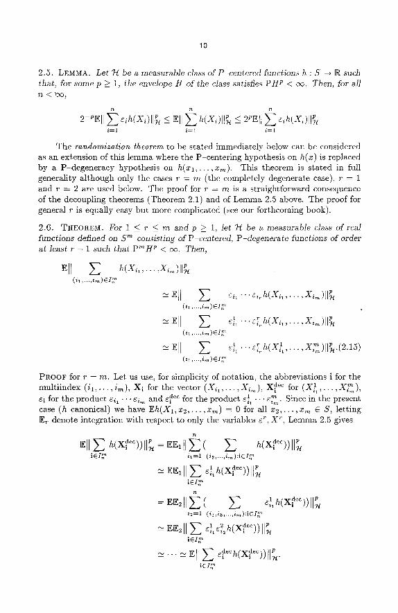
10
2.5. LEMMA. Let 7-( be a measu rab l e class o f P -cen te red functions h : S ~ R such that, for some p > 1, the envelope H of the class satisiqes P H p < oc. Then , for ali rt <'oo,
12
i=1 i=1 i=1
T h e randomization theorem to be s ta ted immedia t e ly below can be cons idered as a n ex tens ion of this l e m m a where the P - c e n t e r i n g hypothes is on h(z) is replaced by a P - d e g e n e r a c y hypothes is on h ( x l , . . . ,zra) . This t heo rem is s t a ted in full genera l i ty a l t hough only the cases r = m ( the complete ly degenera te case), r = 1 and r = 2 are used below. The proof for r = rn is a s t ra ight forward consequence of the deeoupl ing theorems (Theorem 2.1) and of L e m m a 2.5 above. The proof for genera l r is equal ly easy b u t more compl ica ted (see our fo r thcoming book) .
2.6. THEOREM. For 1 <_ r <_ rn a n d p _> 1, let H be a measurable class of reai funct ions de/ /ned on Sra consisting o f P-centered, P-degenerate functions of order at least r - 1 such that PraH p < oc. Then,
(il ,...,im)ES~
_ Ell (il ,..-,ira)EI~
1 "'el h ( X i l , X P (il ..... i~)ezp
1 . . e [ h ( x l , . . x )II .(2.15) (i~ ..... i,~)EI~
PROOF for r = rn. Let us use, for s implic i ty of no t a t i on , the abb rev i a t i ons i for the �9 21 ra m u l t i i n d e x ( i l , . . . , i r a ) , Xl for the vector ( X i ~ , . . . , X i m ) , X f~c for ( i ~ , ' " , X i m ) ,
el for the p roduc t ei~ - �9 �9 a n d e d~c for the p roduc t e I - �9 �9 Ew Since in the present ~1 ~m " case (h canonica l ) we have Eh(X1, x 2 , . . . , X m ) = 0 for all x 2 , . . . , xra E S, l e t t ing E~ deno te i n t eg ra t i on wi th respect to on ly the variables e ~, X ~, L e m m a 2.5 gives
n h(Xl ) ) l i T / : ~ E l l l E ( E h(Xdec))ll~
|E/~ it=l ( i 2 , . . . , i m ) : i E I ~
n = E E 2 1 i E ( E el h(Xde%hllP il ', i J/ 117l
iz=l (il,iZ,...,im):iEI,m~
1 e2 h C X . a ~ l l ~ iCIp

11
Now the equivalences (2.15) for r = m follow by several applications of the decou- pling Theorem 2.1.
[]
c) Randomizat ion of tail probabilities. Let F be a vector space, let the function h : S m --+ F be symmetr ic in its entries and let I = { ( i l , - . . , i m ) E N m : ij # ik for all j # k}. For finite sets A C N we set
h(x,). i E I A A T M
The following e lementary lemma (basically an inclusion-exclusion principle) pro- vides decoupling and randomizat ion of tail probabilities.
2.7. LEMMA. Let Ai, i = 0 , . . . ,rn, be rn + 1 finite disjoint sets of integers, Ai 7 s 0 K i r O, and let A = uim=oAi . Then,
rn! m
E h(xl) = (--1)mSAo + E ( - - 1 ) m-k E SAoUAq U...uA, k �9 iEA1 x - . - x A ~ k = l l < i l < . . . < i k < _ r n
(2.16)
This l emma for A0 = 0 was observed by Ging and Zinn (1994) and for general A0 by Zhang (1996). See these references (or our forthcoming book) for its proof. An almost immedia te consequence of it is the following one sided decoupling and randomizat ion inequality for tail probabilit ies of U-processes (Gin~ and Zinn, 1994).
2.8. THEOREM. Let 7-{ be a measurable class of real functions o n S m , symmetr ic in their entries. Then, (a) For natural numbers no < n, i f Dj are subsets of {no + 1 , . . . , n}, j = 1 , . . . , m,
m and M = no -]- ~ j = l ]Djl, then, for all t > O,
2mt Pr{ll E j
lED1 •215 Dr .
< 2 m max Pr{I I E h ( X i l , . . , xim)ll n > t } ; (2.17) n o < k < M ~ - -
(b) for natural numbers no < n and a/1 t > 0,
2 2 m r - Pr{ll n o < i l , . . . , i r n < n
< 2 2m max P r { I I E h ( X i l , . . . X i m ) l l ~ ) t } . (2.18) n o < k < n m ~ - -
PROOF assuming L e m m a 2.7. Inequality (2.17) is trivially true if Dj = ~ for some j . So, assuming tha t Dj is not empty for any j , we take A0 = { 1 , . . . , n 0 } , Aj =

12
{1 + s 0 + E 21 IDo l , . . . , ~0 + E~=I IDil}, J = 1 , . . . , m, which are disjoint, and note tha t , by pe rmu ta t i on of the factors in the infinite product of (S, $ , P ) ,
. . x TM 2mt/ Pr{ll • h(X:l, , m)ll -> j IED1 x . . .xDm
- - Pr{I I ~ h(X~l, ,X~m)ll > 2rnt~ . . . . r e ! J "
iCAI x.- .xAm
Then, pa r t (a) follows by direct appl ica t ion of Lemma 2.7.
Pa r t (b) follows from par t (a) and Fubini ' s theorem because
E el m h , X 1 X m ~ t ' " c i m ( i t , ' " , i,~) n o ~ _ i l , . . . , i m < n
is a l inear combinat ion with coefficients -t-1 of 2 m terms of the form
Z f(xl, iEDt x. . -xDm
J - 1 } . J 1} or Dj {no < i < n : e i with Dj = {no <: i _< n : e i = = _ = []
It should be noted tha t there is no converse to inequality (2.18) in general, even for m = 1. For instance, if X is such tha t P r { X > t} _~ c l t - l ( l og t ) -~ ( l og log t ) -2 and P r { X < - t } _~ c2 t - l ( l og t ) - l ( l og log t ) -2 as t --~ ec and c 1 ~s c 2 (and o n e
n can find ci's such tha t this r andom variable is even centered), then ~ i = 1 Xi = Op (n(log n log log n) -1) whereas ~i~=1 eiXi = Op (n(log n) -1 (log log n ) - 2 ) . To see this jus t note tha t X is in the domain of a t rae t ion of a 1 s table law with centerings tha t upset the normings, and e X is in the domain of a t t rac t ion of a 1 s table law with eenterings equal to zero and with the same normings (see, e.g., Gin~, Mason and GStze, 1997).
Theorem 2.8 is useful for proving 'converse limit theorems' , tha t is, for deducing in tegrabi l i ty proper t ies of h under the assumpt ion tha t the U s ta t is t ic wi th kernel h satisfies a l imit theorem such as the clt or the lil.
It does not seem tha t Theorem 2.8 follows from decoupling of tai l probabi l i t ies (Theorem 2.2); at any rate, Theorem 2.8 is much more e lementary than Theorem 2.2.
3. L i m i t t h e o r e m s for U - s t a t i s t i c s . If h is integrable, then the U-s t a t i s t i c s (1.1) based on the kernel h form a reverse mart ingale , hence, they converge a.s. and in L1; the l imit is a constant by the Hewi t t -Savage zero-one law and this constant is necessari ly E h ( X 1 , . . . , X m ) by L1 convergence. The law of large numbers was first proved by Hoeffding (1948), but this slick argument belongs to Berk (1966). Gin6 and Zinn (1992) gave an example of a U-s t a t i s t i c with a kernel not in L 1 tha t converges a.s. and the question of finding necessary and sufficient condit ions on h for the U-s t a s t i s t i c s Un(h) to converge (possibly after centering) a.s. or in p robabi l i ty to a constant , is open. For the case h(X l , . . . , Xm) = X l " ' " X m see Cuzick, Gin~ and Zinn (1995) and Zhang (1996). Recent developments on the exact es t imat ion of

13
moments of U-statistics (Klass and Nowicki, 1996) allow" for some optimism, but it is too early to tell.
Similar comments apply to the law of the iterated logarithm, except that it was not known until very recently (Arcones and Ginfi, 1995) that finiteness of the second moment of the kernel implies the lil for the corresponding U statistic in the completely degenerate case and for all ra. The proof of this result does rely heavily on decoupling (Theorem 2.1). Here again, h being in L2 is not a necesary condition for the lil in the canonincal case (Gin~ and Zhang, 1996), and necessary and sufficient conditions are not known.
On the other hand, the tit is completely solved. Sufficiency of square integra- bility of the kernel for a completely degenerate U statistic of order m (for any m) to satisfy the elf was proved by Rubin and Vitale (1980) and necessity by Gin~ and Zinn (1994). Decoupling (Theorem 2.8) plays a basic role in the proof of necessity.
Only the clt and the lil will be described here. As a consequence of Hoeffding's decomposition (2.13), (2.14), it is clear that, at least under some integrability for h, the clt (resp. the lil) for the completely degenerate or canonical case give the clt (resp. the lil) in general. So, only canonical kernels will be considered.
a) The central limit theorem. Let Xi be i.i.d, centered random variables, with finite second moment equal to 1. Then, the elf and the lln for sums of i.i.d, random variables gives
1 X i X j 1 X i X 2 ---+d 1, r~ 7Z
(i,j)eI~ i = 1 i = 1
where g is N(0, 1). This is the clt for the U-statistics with kernel h(x, y) = xy, which is degenerate if EX1 = 0. This simple example is very appropriate because canonical kernels are just limits in L2 of linear combinations of products r r q5 P-centered. Extrapolating, the example suggests that a canonical U-statistic of m variables, multiplied by n"qz, should converge in law to an element of a Gaussian chaos of order ra. This is the content of the direct clt for canonical U-statistics, which we now describe for completeness and also for use in the next section.
Let L~(5',,5, P) be the space of real valued P-centered, P-square integrable functions on o% Let Gp be an isonormal Gaussian process on L~(S, S, P), that is, a centered Gaussian process with parameter set L~(S, $, P) such that EGp(f)Gp(g) = f fgdP. If {r is an orthonormal basis of L~(S, $, P) and if {gi}ie[ is a family of independent N(0, 1) random variables, then the equation
2
iEI iEI iEI
produces such a process. By identifying random variables which are a.s. equal, Gp becomes a linear isometry from L~(S, S, P) onto the Hilbert space of jointly normal random variables generated by {Gp(f)} (or, isomorphically, by the gi's). Then, the finite dimensional central limit theorem simply asserts that the finite dimensional distributions of the processes { ~ ~i~1 f (Xi): f C L~(S, S, P)}, converge in law
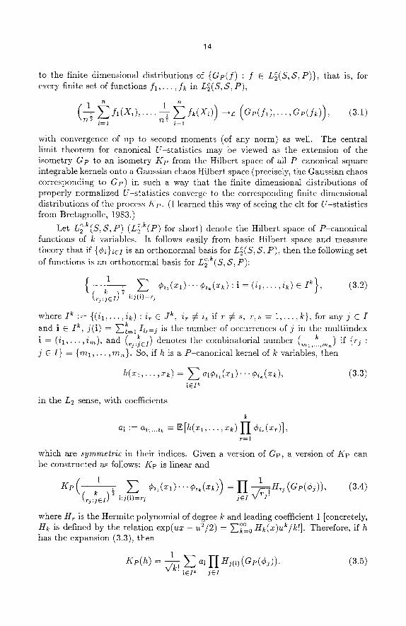
14
to the finite dimensional distributions of {Gp(f) : f E L~(S ,N,P)} , that is, for every finite set of functions f l , . . . , fk in L~(S, $, P) ,
( ~ ~-~fl(Xi) ' 1 ~ )) ( )) �9 . . ~ - f k ( X i --+c G e ( f l ) , . . . , G p ( A , (3.1)
Tt'ff i=1 rt2 i=1
with convergence of up to second moments (of any norm) as well. The central limit theorem for canonical U statistics may be viewed as the extension of the isometry Gp to an isometry Kp from the Hilbert space of all P canonical square integrable kernels onto a Gaussian chaos Hilbert space (precisely, the Gaussian chaos corresponding to Gp) in such a way that the finite dimensional distributions of properly normalized U statistics converge to the corresponding finite dimensional distributions of the process Kp. (I learned this way of seeing the elf for U-stat ist ics from Bretagnolle, 1983.)
Let L~'k(S,S, P) (L~'k(P) for short) denote the Hilbert space of P-canonica l functions of k variables. It follows easily from basic Hilbert space and measure theory that if {r162 is an orthonormal basis for L~(S, S, P), then the following set of functions is an orthonormal basis for L~'k(s, 3 , P) :
1 { k �89 ~ ~il(Xl)' ' 'r _fk}, ( 3 . 2 )
(rj:jeI) i:j(i)=rj
where I k := { ( i l , - . . , i k ) : ir C jk , iT # i8 if r # s, r , s = 1 , . . . , k}, for any j C I
and i �9 I k, j ( i ) = }-~-~=1 Ii,=j is the number of occurrences of j in the multiindex
i = ( /1 , . . . , i r a ) , and (rj:~El) denotes the combinatorial number ( . . . . k.,mn) if {rj : j �9 I} = { r n l , . . . , ran}. So, if h is a P-canonical kernel of k variables, then
h(xl,...,Xk) = ~ air162 ( 3 . 3 ) IEI k
in the L2 sense, with coefficients
k
al := ait...ik = E [ h ( x l , . . . , x k ) I I r r=l
which are ~ymmetric in their indices. Given a version of Gp, a version of Ifp can be constructed as follows: Kp is linear and
( 1 ~ r 1 H - . . . . I I ( 3 . 4 ) (rj:~EI) 7 i:j(i)=rd jC=I V ' 3"
where HT is the Hermite polynomial of degree k and leading coefficient 1 [concretely, Hk is defined by the relation exp(ux - u2/2) = ~k~__0 Hk(x)uk/k[]. Therefore, if h has the expansion (3.3), then
1 I I Hi(1)(Gp(r (3.5) Kp(h) = ~ . ~ al iEI k jEI
15
We call Kp the isonormal Gaussian chaos process associated to the Gaussian process Gp (and will shortly explain why). Then, the Rubin and Vitale (1980) central limit theorem can be stated as follows:
3.1. THEOREM. For arbritrary natural numbers rt, 1 <_ g <_ k < o% let ht be P-square integrable, P-canonical kernels in rt variables (that is, ht E L 2 (P)), and let Kp be an isonormal Gaussian chaos process on O~=lL2 (P). Then,
1 1
~Un(hl),..., U~(hk) - ~ • (3.6) r l r k
as n ---+ oo, with convergence of up to second moments of the norm.
In fact, this limit theorem admits an extension to finite numbers of functions oo c~k in @k=lL2 (P). For a single function h E | the result is that, if h =
Y~k~__l hk with hk E L~'k(P), then
k = l
(Dynkin and Mandelbaum, 1983).
Let (ft, E, Pr) be the probability space where the isonormal process Gp is de- fined, and let a(Gp) be the sub-a-a lgebra of E generated by the random variables {Gp(r : r E L~(P)}. Then L2(Gp) := L 2 ( ~ , a ( G p ) , P r ) is the Hilbert space of square integrable Gp measurable functions. Let "Pk(Gp) ('Pk for short) be the Hilbert subspace of L2(Gp) generated by the polynomials of degree at most k in the variables Gp(r r E L~(P), and let 7-tk(ae) (~k for short) be the orthogonal complement of Pk-1 in Pk, that is,
7-tk = Pk O Pk-1.
It turns out that Kp, extended as the identity on constants, is an isometry from the Hilbert subspace of L2(SN,P N) generated by the constants and the canonical
kernels of all orders, I~ | Gk=IL2 (P) (note that all these spaces are orthogonal
in L2(S N, pN)), onto L2(Gp) = | ~k(P5 such that
Kp(L~'k(P)) = 7-{k(P), k E N, (3.7)
In other words, the orthogonal decomposition into canonical kernels of different orders induces, via Kp, the chaos decomposition of L2(Gp). This justifies the name given to the process Kp. We note that it is possible to simultaneously prove the clt for U statistics and the chaos decomposition of L2(Gp), quite economically. See our forthcomming book for details. For a similar abbreviated account of the same theory see Bretagnolle (1983). Dynkin and Mandelbaum (1983) contains another derivation of the same facts.Theorem 3.1 was first proved for m = 2 by Serfling (1980) and Gregory (1977).
Theorem 3.1 has the following converse (Gin6 and Zinn, 1994):
16
3.2. THEOREM. Let h : S k ~ R be a measurable symmetr ic function on ( S , S ) and let X , X i , i C N, be i.i.d. S-valued random variables with probabili ty law P. I f the sequence of random variables
is stochastically bounded, then E h 2 ( X 1 , . . . , X k ) < oo and, moreover, h is P canonical.
Here is a sketch of the proof. By Theorem 2.8 on deeoupling and randomization, stochastic boundedness of the sequence (3.8) implies stochastic boundedness of the sequence of decoupled and randomized U-statistics
l_~il,...,i~_~n
It then follows from this and properties of Rademacher multilinear forms that the sequence
l <_il ,...,ik <_n
is also stochastically bounded. But then, by positivity, so is the family of variables
Z ): N,c > o , . . . ~ z k
l <_il ,...,ik <_n
Now, this and the law of large numbers for U statistics applied to the bounded kernels h 2 Ih 2_<c imply that the numbers E [(h 2 Ih2 <_c)(Xl , . . . , Zk)] are bounded uni- formly in c, hence, that Ehe(X1, . . . , Xk) < oo. This, the direct clt and Hoeffding's decomposition yield that h is P-canonical. [The property of Rademacher multilinear forms used here is that their fourth moment is dominated by a universal constant times the square of their second moment, which is elementary, in fact very easy to check in the decoupled case; this then allows use of the Paley-Zygmund argument (Kahane, 1968, page 6), conditionally on the X's, to obtain tightness of the sums of squares.]
We complete this section with the observation that Theorem 3.1, the central limit theorem for U statistics in several dimensions, can be used in conjunction with Theorem 2.2, decoupling of tail probabilities for U-statistics, to produce a comparison theorem for tail probabilities of Gaussian polynomials and their decou- pled versions. The result is as follows. For ease of notation we set lil := maxt it.
Given a sequence {gi : i E N} of i.i.d. N(0, 1) random variables and a polyno- mial Q(m) of degree m in the variables gi, and with coefficients in a Banach space B, with expansion
k = O max~_<,~ l i~ l < N j EN
17
where the coefficients al are symmetric in their indices (which we can assume without any loss of generality), its decoupled version is defined as
m
k = O . . . . <_t: [i~l<_N jEIkm
by arcones and Gin~ (1993@ whcre {g}J) : i e N}, j = 1 , . . . , m, are rn independent copies of the sequence {gi}. With this definition, we have:
3.3. TIIEOREM. For each m E N there exists Cm E (0, oo) such that, if B is a Banach space, Q(m) is a Gaussian polynomiM of degree rn in an orthogaussian sequence {gi}, with coettlcients in B, and o&c is its decoupled version, then "~(m)
I Pr{llQ(a&~)l I > Crnt} ~ Pr{llQ(m)][ > t} < CmPr{ dec C m - - - - "
Since the constant Cm is independent of N, the theorem extends to the whole Gaussian chaos of order m (for each m). This is a generalization (Arcones and Gin4, 1993, and Ginfi, 1997) of a theorem of Kwapiefi (1987) for homogeneous polynomials in {gi} of degree at most one in each gi.
The proof consists in observing that Q(m) is the limit in law of a U-statistic with values in the finite dimensional space generated by the (finite number of) coefficients al, and that g)g~c is the limit in law of the corresponding decoupled U-statistics, "~(m) so that the theorem follows by taking limits in the inequality of Theorem 2.2. [This simple proof would not be possible without Theorem 2.2; Kwapiefi (1987) developed very effective and elegant tools to prove the version of Theorem 3.3 for homogeneous tetrahedral polynomials and the version of Corollary 2.3 above for expected values of convex functions and symmetric variables, and some of these tools made their way into the proof of Theorem 2.2.]
b) The law of the iterated logarithm. As with the clt, in order to guess the natural norming in the lil for degenerate U statistics, it is instructive to begin with the simplest example, namely the kernel h(x,y) = xy and random variables Xi i.i.d. with EXi = 0 and EX~ = 1. Then, the Hartman-Wintner lil for sums of i.i.d. square integrable random variables and the law of large numbers readily show that
limnSUp 2n 1 E XIXj log log n
n �9 / t
z 1 = l imsup 2nlo ogn)�89 Xi 2nloglogn i
i = 1 i = 1
In fact, by Strassen's lil (e.g. Ledoux and Talagrand, 1991, page 206), for almost every w, the set of limit points of the sequence { y-~qX Xi(co)Xj(w)/2n log log n } ~--1 is precisely the interval [0, 1]. This is just a particular case of a more general statement: the kernel xy is replaced by a general square integrable P-canonical kernel in m variables, the norming 2nloglogn is replaced by a . = (2nloglogn) ml2, and the limit set [0, 1] becomes the set {E[h(X1, . . . ,Xm)g(X1)" .g(Xm)] : Eg2(X1) _< 1}.

18
Decoupling and randomiza t ion , together with the hypercont rac t iv i ty p rope r ty of Rademacher chaos, will be seen to provide an elegant pa th towards this result .
Con t ra ry to the case of sums of i.i.d, random variables, square in tegrabi l i ty of the kernel is not a necessary condit ion for the lil when m >_ 2. However, it is neces- sary when h is res t r ic ted to be of a par t icu lar type, and there is a necessary condi t ion for the LIL in te rms of in tegrabi l i ty of h which differs from square in tegrabi l i ty only by a power of log log Ihl.
To ease nota t ion , given h : S m --+ IR, we set
1 a~(h) := (2n log log n) ~ E h(X i~ , . . . ,X i , , ) . (3.9)
(i, ..... im)eIn T M
The lil for canonical U s ta t is t ics is then as follows:
3.4. THEOREM. Let X , Xi , i E N, be i.i.d, random variables with values in a measurab le space ( S , S ) and common law P. Let hj : S m --+ N be P canonical functions with Eh~ < oo, j = 1 , . . . , d. Then, with probability one, the sequence
{ (3.10)
is relatively compact in R d and its limit set is
: : {]E[g(Xl)-..g(Xm)(hl(Xl,... ,Xrn ) , . . . , h d ( X l , . . . ,Kin))] : Eg2(X) ~ 1}. K
(3.11)
This theorem is due to Dehling (1989) for m = 2 and to Arcones and Gin6 (1995) for general m. Dehling and Utev (to appear) gives a sketch of a proof of Theorem 3.4 for general m and d = I, different from ours.
The main point in our proof consists in obtaining the following intermediate proposition (the bounded ill):
3.5. PROPOSITION. Let (S',,5",P) be a probability space, let Xi , i E N, be i.i.d. r andom variables with values in S and law P, and let h : S m --+ R be a P-canonical kernel such that gh 2 < oo. Then, for every 0 < p < 2, there exists a constant Cm,p < oo depending only on m and p such that
E s u p [ 1 n)m/2 E h ( X i l " " ' X i ' ~ ) ] p h e n L (2n log log (i ...... ira) eI~
< Cm,p(IEh2(Xl , . . . , X m ) ) ~. (3.12)
(3.3) and polar iza t ion imply tha t the set of finite l inear combinat ions of func- tions of the form
h ~ ( x l , . . . , X m ) : : r , / r fr (3.13)
19
is dense in L~"~(P). Then, Proposition 3.5 reduces the proof of Theorem 3.4, by means of a s tandard approximation argument, to the lil for kernels of the form
k
h = E c'h~m" (3.14) r ~ l
The lil (i.e., Theorem 3.4) for U-statist ics with kernels of the form (3.14) is an immediate consequence of Strassen's lil for sums of R d valued i.i.d, random variables. Here is how it works for rn = 2 and d = 1. Strassen's lil (e.g., Ledoux and Talagrand, 1991) asserts that if Y , Yi, i E N, are i.i.d, random vectors in R k, then, the sequence
1
(2n log log n) �89
is relatively compact for almost every w E and then
{ 1 lim set (2n log log n) �89
where K y is the subset of ]1{ k defined by
n oG
/ ~ 1 Y i (('~ } n = l "=
ft if and only if E Y = 0 and EIYI 2 < oe,
n
i=1
K y : { E [ ( g ( Y ) ) Y ] : g real, measurable, and Eg2(Y) < 1}.
Hence, if r i = 1 , . . . , k, are centered and square integrable, we have
n
lim set~ 1_ 1 E ( @ I ( X j ) , . . . , ~ ) k ( X j ) ) } t (2n log logn)~ j=l
= : Eg2(X) _< 1},
where we take this statement to mean that, moreover, the sequence in question is relatively compact with probability one, and where X is a random variable with
k law P. Then, applying the continuous function ~(x l , . . . , xk) ~ r = l c,x~ to both terms, we obtain
~, r 2 2n log log n
r = l j = l
k
= {Ecr [Er 1}. (3.15)
Now, with h as in (3.14) and rn = 2,
1 E C r ( E r - 2711oglogTt l<i,j<n 2n loglog n ~=1 j=]
1 2n log logn ~ h(Xi ,Xj ) +
1 h(x~, xi), 2n log log n i=1

20
and the last summand tends to zero a.s. by the law of large numbers since E l h ( X l , X ~ ) l < ~ Ic~lEr < oc. Moreover,
k k E cr [ E~)r(x)g(X)]2 : E Cr~ [I/)r(X1 )l/)r(X2 )g(Xl )g(X2 )] r=l r=l
= E [h(X1, X2 )9(21 )9(22 )].
Hence, (3.15) becomes
limset{2 1 Eh X ,Xj } = {EEh(Xl,X2 g(Xl)g(X2 l : 1}, log log r[ r2
that is, the lil in Theorem 3.4 for the simple function h given by (3.14). The proof for m > 2 is slightly more involved, and Newton's identities help to account for the sums with repeated Xi ' s in the analogue of the identity below (3.15).
We next see how" to obtain the basic inequality (3.12) in Proposit ion 3.5 by indicating several steps.
Step 1: DecoupIing and randomization. Let K be a natural number and let 0 < p < 2. Lett ing t~, = (0, r.-1.)O, h/ar, h / a r + l , . . . , h/a2K) E ~2~, it is easy to see that
Z h(xl) = h,(xl) n I ~ x I
So, we can apply Theorem 2.1 for f ~ valued kernels (which can be viewed as a family of real valued kernels, as indicated immediately below the proof of Theorem 2.1) and obtain
E h(Xi) P 1 E d . . . . . . decx p E m a x < C E m a x s i n tA i ) n < 2 K n ~ 2 K
- i E I ~ '~ - i E l $
for some constant C < oo depending only on m and p.
Step 2: Blocking. Blocking is an essential part of the proof of the Ill for sums of i.i.d. random variables, and it is achieved via maximal inequalities (L6vy or Ottaviani). Once the statistic is decoupled and randomized, we can apply L@vy's inequalities
J J N}, repeatedly, and conditionally on all but one of the m sequences { s i , X i : i E obtain
1 E d . . . . . . aecxl p 1 E d . . . . . . dec,[ p E m a x - gl n [~ i )[ < 2 m E max ~ El nk~i ) 1 ' n<2 K _ an iEi. m k<K--l_ a k iEI~+l
where a~ := a2k. We axe now prepared for application of a basic property of Rademacher multilinear forms.
Step 3a: A maximal inequality. Let r on N+ U {0} be a Young modulus that is, a real function such that r = 0 and ~b is convex and strictly increasing to infinity.

21
Then, the space Lr E, Pr) of all the random variables ~ defined on f~ such that Er < ~ f o r some 0 < c < 0% equipped with the norm
I1~11r = inf{c > O: Er _< 1},
is a Banaeh space (of. Krasnoselsky and Rutitsky, 1961). For instance, if r = x p, 1 < p < 0% then I1~11~ = II~llp We are more intersted in Young functions of exponential type, g?~, 0 < c~ < 0% which are defined as follows:
r Tc~(X)--c~exp , i f0 <c~ < t,
1
where , . ( x ) denotes exp(x ~) if x _> ( ~ ) ; , and it denotes the (ordinate of)
((-:) tangent line to the fmlction y = exp(x ~) at the point z exp if 0 _< 1
(k~__~) ;-. (The complication in the definition of ~b~ for ~ < 1 is due to the fact X <
that the function y = exp(x ~) is not convex near zero.) Note that for all p > 0 and all a > 0 there is cp,~ < ec such that
II~llp -< cp,~ll~II,o.
We can now state a useful maximal inequality (Arcones and Gind, 1995), valid for Young moduli slightly more general than ~a, but not for power moctuli.
3.6. PROPOSITION. Let ~ be a Young modulus such that
~ ) - - l ( x y ) l imsup r < co (3.16) :cAy----~ ( x ) r
and
r ) < ~ . (3.17) limsup~oo r
Then, there exists a finite constant C~ such that, for every sequence of random variables {~k : k C N},
sup ICkl < CcsupllCkll,. (3.18) k ~----2~(k) r - k
This inequality is good for us because of the following property of Rademacher chaos variables:
Step 3b: Integrability (hypercontractivity) of Rademacher ~um~. If Y = ~ aici, it is classical (Bonami, 1970) that
l'~1/2(V'a2"~l/2 ( E I Y F ) I / p < ( P - , ,z_., ~J ' P >-2"
Conditionally applying this inequality to the decoupled Rademacher m-l inear form
E 1 , . s Z = a i l . . . i m s " ~ m '
i l ~...~im


