145
Lecture Notes on ELECTROMAGNETIC FIELDS AND WAVES (227-0052-10L) Prof. Dr. Lukas Novotny ETH Z ¨ urich, Photonics Laboratory February 9, 2013

Lecture Notes on
ELECTROMAGNETIC FIELDS AND WAVES
(227-0052-10L)
Prof. Dr. Lukas Novotny
ETH Zurich, Photonics Laboratory
February 9, 2013

Introduction
The properties of electromagnetic fields and waves are most commonly discussed
in terms of the electric field E(r, t) and the magnetic induction field B(r, t). The
vector r denotes the location in space where the fields are evaluated. Similarly, t
is the time at which the fields are evaluated. Note that the choice of E and B is ar-
bitrary and that one could also proceed with combinations of the two, for example,
with the vector and scalar potentials A and φ, respectively.
The fields E and B have been originally introduced to escape the dilemma of
“action-at-distance’, that is, the question of how forces are transferred between
two separate locations in space. To illustrate this, consider the situation depicted
in Figure 1. If we shake a charge at r1 then a charge at location r2 will respond.
But how did this action travel from r1 to r2? Various explanations were developed
over the years, for example, by postulating an aether that fills all space and that
acts as a transport medium, similar to water waves. The fields E and B are pure
constructs to deal with the “action-at-distance’ problem. Thus, forces generated by
q2
q1
r2
r1
?
Figure 1: Illustration of “action-at-distance”. Shaking a charge at r1 makes a sec-
ond charge at r2 respond.
1
2
electrical charges and currents are explained in terms of E and B, quantities that
we cannot measure directly.
Basic Properties
As mentioned above, E and B have been introduced to explain forces acting on
charges and currents. The Coulomb force (electric force) is mediated by the elec-
tric field and acts on the charge q, that is, Fe = qE. It accounts for the attraction or
repulsion between static charges. The interaction of static charges is referred to
as electrostatics. On the other hand, the Lorentz force (magnetic force) accounts
for the interaction between static currents (charges traveling at constant velocities
v = r) according to Fm = qv × B. The interaction of static currents is referred to
as magnetostatics. Taken the electric and magnetic forces together we arrive at
F(r, t) = q [E(r, t) + v(r, t) × B(r, t)] (1)
In the SI unit system, force is measured in Newtons (N = J / m = A V s / m) and
charge in terms of Coulomb (Cb = A s). Eq. (1) therefore imposes the following
units on the fields: [E] = V/m and [B] = V s / m2. The latter is also referred to as
Tesla (T).
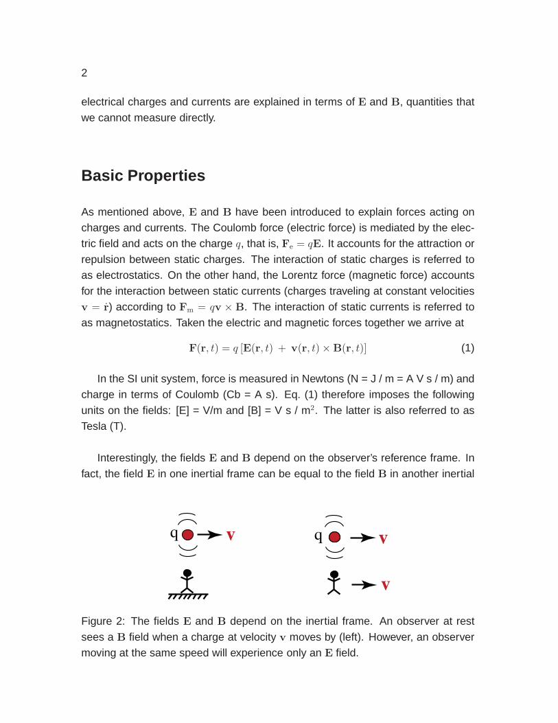
Interestingly, the fields E and B depend on the observer’s reference frame. In
fact, the field E in one inertial frame can be equal to the field B in another inertial
qq v v
v
Figure 2: The fields E and B depend on the inertial frame. An observer at rest
sees a B field when a charge at velocity v moves by (left). However, an observer
moving at the same speed will experience only an E field.

3
frame. To illustrate this consider the two situations shown in Figure 2 where an
observer is measuring the fields of a charge moving at velocity v. An observer at
rest will measure a B field whereas an observer moving at the same speed as the
charge will only experience only an E field. Why? Because the charge appears to
be at rest from the observer’s point of view.
In general, the electric field measured by an observer at ro and at time t can be
expressed as (see R. Feynman ‘Lectures on Physics’, Vol. II, p 21-1)
E(ro, t) =q
4πε0
[
nr′
r′2+
r′
c
d
dt
(nr′
r′2
)
+1
c2d2
dt2nr′
]
, (2)
where c = 2.99792456 .. 108 m/s is the speed of light. As shown in Figure 3, r′ is the
distance between the charge and the observer at the earlier time (t − r′/c). Simi-
larly, nr′ is the unit vector point from the charge towards the observer at the earlier
time (t− r′/c). Thus, the field at the observation point ro at the time t depends on
the motion of the charge at the earlier time (t− r′/c)! The reason is that it takes a
time ∆t = r′/c for the field to travel the distance r′ to the observer.
Let us understand the different terms in Eq. (2). The first term is proportional
to the position of the charge and describes a retarded Coulomb field. The second
term is proportional to the velocity of the charge. Together with the first term it
describes the instantaneous Coulomb field. The third term is proportional to the
acceleration of the charge and is associated with electromagnetic radiation.
position at t- r’/cposition at t
rq
q
E(ro, t)
nr’
r’
Figure 3: The field at the observation point ro at the time t depends on the motion
of the charge at the earlier time (t− r′/c).

4
The objective of this course is to establish the theoretical foundations that lead
to Eq. (2) and to develop an understanding for the generation and propagation of
electromagnetic fields.
Microscopic and Macroscopic Electromagnetism
In microscopic electromagnetism one deals with discrete point charges qi located
at rn (see Figure 4). The charge density ρ and the current density j are then
expressed as sums over Dirac delta functions
ρ(r) =∑
n
qn δ[r − rn] , (3)
j(r) =∑
n
qn rn δ[r − rn] , (4)
where rn denotes the position vector of the nth charge and rn = vn its velocity. The
total charge and current of the particle are obtained by a volume integration over ρ
and j. In terms of ρ and j, the force law in Eq.(1) can be written as
F(r, t) =
∫
V
[ρ(r, t)E(r, t) + j(r, t) × B(r, t)] dV (5)
where V is the volume that contains all the charges qn.
qn
rn r
Figure 4: In the microscopic picture, optical radiation interacts with the discrete
charges qn of matter.
5
In macroscopic electromagnetism, ρ and j are viewed as continuous functions
of position. Thus, the microscopic structure of matter is not considered and the
fields become local spatial averages over microscopic fields. This is similar to the
flow of water, for which the atomic scale is irrelevant.
In this course we will predominantly consider macroscopic fields for which ρ
and j are smooth functions in space. However, the discrete nature can always be
recovered by substituting Eqs. (4).
Pre-Maxwellian Electrodynamics
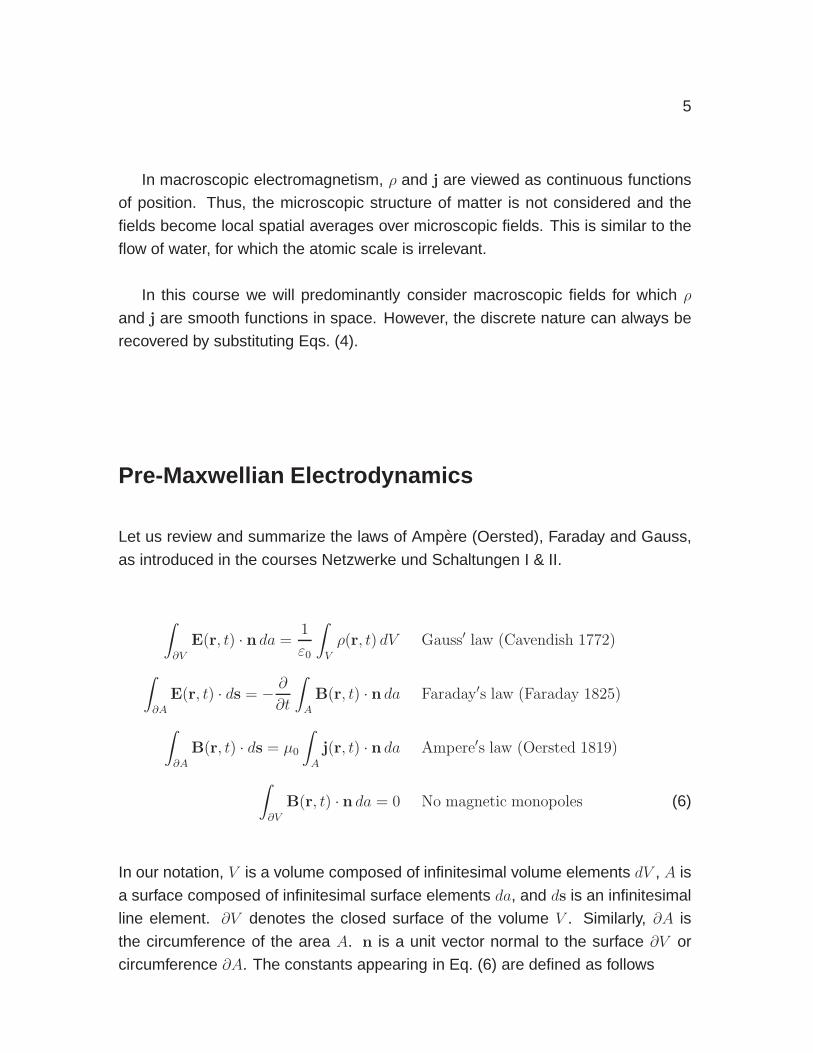
Let us review and summarize the laws of Ampere (Oersted), Faraday and Gauss,
as introduced in the courses Netzwerke und Schaltungen I & II.
∫
∂V
E(r, t) · n da =1
ε0
∫
V
ρ(r, t) dV Gauss′ law (Cavendish 1772)
∫
∂A
E(r, t) · ds = − ∂
∂t
∫
A
B(r, t) · n da Faraday′s law (Faraday 1825)
∫
∂A
B(r, t) · ds = µ0
∫
A
j(r, t) · n da Ampere′s law (Oersted 1819)
∫
∂V
B(r, t) · n da = 0 No magnetic monopoles (6)
In our notation, V is a volume composed of infinitesimal volume elements dV , A is
a surface composed of infinitesimal surface elements da, and ds is an infinitesimal
line element. ∂V denotes the closed surface of the volume V . Similarly, ∂A is
the circumference of the area A. n is a unit vector normal to the surface ∂V or
circumference ∂A. The constants appearing in Eq. (6) are defined as follows

6
µ0 = 4π 10−7 Vs
Am= 1.2566370 10−6 Vs
Am(magnetic permeability)
ε0 =1
µ0 c2= 8.8541878 10−12 As
Vm(electric permittivity)
where c = 2.99792458 108 m/s is the vacuum speed of light. Fig. 5 illustrates the
meaning of the four equations (6). The first equation, Gauss’ law, states that the
flux of electric field through a closed surface ∂V is equal to the total charge q
inside ∂V . The second equation, Faraday’s law, predicts that the electric field in-
tegrated along a loop ∂A corresponds to the time rate of change of the magnetic
flux through the loop. Similarly, Ampere’s law, states that the magnetic field inte-
grated along a loop ∂A is equal to the current flowing through the loop. Finally, the
fourth equation states that the flux of magnetic field through a closed surface is al-
ways zero which, in a analogy to Gauss’ law, indicates that there are no magnetic
charges.
q1
q2
q3
V
Ea
BA∂
∂t
E ds
b
B ds
jcd
VA
B
Figure 5: Illustration of (a) Gauss’ law, (b) Faraday’s law, (c) Ampere’s law, and (d)
the non-existence of magnetic charges.

7
B
Figure 6: Ampere’s law applied to a cube. Opposite faces cancel the magnetic
circulation∫
∂AB(r, t) · ds, predicting that the flux of current through any closed
surface is zero.
Let us consider Ampere’s law for the different end faces of a small cube (c.f.
Fig. 6). 1 It turns out that the magnetic field integrated along the circumference of
one end face (∫
∂AB(r, t) · ds) is just the negative of the magnetic field integrated
along the circumference of the opposite end face. Thus, the combined flux is zero.
The same is true for the other pairs of end faces. Therefore, for any closed surface
Ampere’s law reduces to∫
∂V
j(r, t) · n da = 0 Kirchhoff I . (7)
In other words, the flux of current through any closed surface is zero, - what flows
in has to flow out.
Eq. (7) defines the familiar current law of Kirchhoff (Knotenregel). On the other
hand, Kirchhoff’s voltage law (Maschenregel) follows from Faraday’s law if no time-
varying magnetic fields are present. In this case,∫
∂A
E(r, t) · ds = 0 Kirchhoff II . (8)
The two Kirchhoff laws form the basis for circuit theory and electronic design.
1An arbitrary volume can be viewed as a sum over infinitesimal cubes.

8

Chapter 1
Maxwell’s Equations
Equations (6) summarize the knowledge of electromagnetism as it was understood
by the mid 19th century. In 1873, however, James Clerk Maxwell introduced a crit-
ical modification that kick-started an era of wireless communication.
1.1 The Displacement Current
Eq. (7) is a statement of current conservation, that is, currents cannot be generated
or destroyed, the net flux through a closed surface is zero. However, this law
is flawed. For example, let’s take a bunch of identical charges and hold them
together (see Fig. 1.1). Once released, the charges will speed out because of
Coulomb repulsion and there will be a net outward current. Evidently, the outward
current is balanced by the decrease of charge inside the enclosing surface ∂V ,
and hence, Eq. (7) has to be corrected as follows
∫
∂V
j(r, t) · n da = − ∂
∂t
∫
V
ρ(r, t) dV (1.1)
This equation describes the conservation of charge. It’s general form is found in
many different contexts in physics and we will encounter it again when we discuss
the conservation of energy (Poynting theorem).
Because Eq. (7) has been derived from Ampere’s law, we need to modify the
9

10 CHAPTER 1. MAXWELL’S EQUATIONS
latter in order to end up with the correct conservation law of Eq. (1.1). This is where
Maxwell comes in. He added an additional term to Ampere’s law and arrived at
∫
∂A
B(r, t) · ds = µ0
∫
A
j(r, t) · n da +1
c2∂
∂t
∫
A
E(r, t) · n da , (1.2)
where 1/c2 = ε0µ0. The last term has the form of a time-varying current. Therefore,
ε0 ∂E/∂t is referred to as the displacement current.
We again apply this equation to the end faces of a small cube (c.f. Fig. 6) and,
as before, the left hand side vanishes. Thus,
µ0
∫
∂V
j(r, t) · n da +1
c2∂
∂t
∫
∂V
E(r, t) · n da = 0 . (1.3)
Substituting Gauss’ law from Eq. (6) for the second expression yields the desired
charge continuity equation (1.1).
In summary, replacing Ampere’s law in (6) by Eq. (1.2) yields a set of four equa-
tions for the fields E and B that are consistent with the charge continuity equation.
These four equations define what is called Maxwell’s integral equations.
t = 0 t > 0
e-
e-
e-
e-
e-
e-e
-
e-
e-
e-
e-
e-
e-
e- e
-e
-
e-
e-
e-
e-
e-
Figure 1.1: Illustration of charge conservation. A bunch of identical charges is
held together at t = 0. Once released, the charges will spread out due to Coulomb
repulsion, which gives rise to a net outward current flow.

1.2. INTERACTION OF FIELDS WITH MATTER 11
1.2 Interaction of Fields with Matter
So far we have discussed the properties of the fields E and B in free space. The
sources of these fields are charges ρ and currents j, so-called primary sources.
However, E and B can also interact with materials and generate induced charges
and currents. These are then called secondary sources.
To account for these secondary sources we write
ρtot = ρ + ρpol , (1.4)
where ρ is the charge density associated with primary sources. It is assumed that
these sources are not affected by the fields E and B. On the other hand, ρpol is
the charge density induced in matter through the interaction with the electric field.
It is referred to as the polarization charge density.1 On a microscopic scale, the
electric field slightly distorts the atomic orbitals in the material (see Fig. 1.2). On a
macroscopic scale, this results in an accumulation of charges at the surface of the
material (see Fig. 1.3). The net charge density inside the material remains zero.
To account for polarization charges we introduce the polarization P which, in
analogy to Gauss’ law in Eq. (6), is defined as∫
∂V
P(r, t) · n da = −∫
V
ρpol(r, t) dV . (1.5)
P has units of Cb/m2, which corresponds to dipole moment (Cb / m) per unit vol-
1The B-field interacts only with currents and not with charges.
nucleus electron orbital
ba
+ +-
-
Figure 1.2: Microscopic polarization. An external electric field E distorts the orbital
of an atom. (a) Situation with no external field. (b) Situation with external field.

12 CHAPTER 1. MAXWELL’S EQUATIONS
ume (m3). Inserting Eqs. (1.4) and (1.5) into Gauss’ law yields∫
∂V
[ε0E(r, t) + P(r, t)] · n da =
∫
V
ρ(r, t) dV . (1.6)
The expression in brackets is called the electric displacement
D = ε0E + P . (1.7)
Time-varying polarization charges give rise to polarization currents. To see this,
we take the time-derivative of Eq. (1.5) and obtain∫
∂V
∂
∂tP(r, t) · n da =
∂
∂t
∫
V
ρpol(r, t) dV , (1.8)
which has the same appearance as the charge conservation law (1.1). Thus, we
identify ∂P/∂t as the polarization current density
jpol(r, t) =∂
∂tP(r, t) . (1.9)
To summarize, the interaction of the E-field with matter gives rise to polarization
charges and polarization currents. The magnitude and the dynamics of these sec-
ondary sources depends on the material properties [P = f(E)], which is the sub-
ject of solid-state physics.
An electric field interacting with matter not only gives rise to polarization cur-
rents but also to conduction currents. We will denote the conduction current den-
sity as jcond. Furthermore, according to Ampere’s law, the interaction of matter with
ρpol
no net charge
−ρpol
ba+-
++
+++
-
--
--
+
-++
+++
----
-
+
--
+++++ -
+++ -
Figure 1.3: Macroscopic polarization. An external electric field E accumulates
charges at the surface of an object. (a) Situation with no external field. (b) Situation
with external field.

1.2. INTERACTION OF FIELDS WITH MATTER 13
magnetic fields can induce magnetization currents. We will denote the magneti-
zation current density as jmag. Taken all together, the total current density can be
written as
jtot(r, t) = j0(r, t) + jcond(r, t) + jpol(r, t) + jmag(r, t) , (1.10)
where j0 is the source current density. In the following we will not distinguish
between source current and conduction current and combine the two as
j(r, t) = j0(r, t) + jcond(r, t) . (1.11)
j is simply the current density due to free charges, no matter whether primary or
secondary. On the other hand, jpol is the current density due to bound charges,
that is, charges that experience a restoring force to a point of origin. Finally, jmag is
the current density due to circulating charges, associated with magnetic moments.
We now introduce (1.10) into Ampere’s modified law (1.2) and obtain
∫
∂A
B · ds = µ0
∫
A
[
j +
(
jpol + ε0∂
∂tE
)
+ jmag
]
· n da , (1.12)
where we have skipped the arguments (r, t) for simplicity. According to Eqs. (1.9)
and (1.7), the term inside the round brackets is equal to ∂D/∂t. To relate the
induced magnetization current to the B-field we define in analogy to Eq. (1.5)
∫
∂A
M(r, t) · ds =
∫
A
jmag(r, t) · n da , (1.13)
with M being the magnetization. Inserting into Eq. (1.12) and rearranging terms
leads to∫
∂A
[
1
µ0B− M
]
· ds =
∫
A
[
j +∂
∂tD
]
· n da , (1.14)
The expression in brackets on the left hand side is called the magnetic field
H =1
µ0B −M . (1.15)
It has units of A/m. The magnitude and the dynamics of magnetization currents
depends on the specific material properties [M = f(B)].

14 CHAPTER 1. MAXWELL’S EQUATIONS
1.3 Maxwell’s Equations in Integral Form
Let us now summarize our knowledge electromagnetism. Accounting for Maxwell’s
displacement current and for secondary sources (conduction, polarization and
magnetization) turns our previous set of four equations (6) into
∫
∂V
D(r, t) · n da =
∫
V
ρ(r, t) dV
∫
∂A
E(r, t) · ds = − ∂
∂t
∫
A
B(r, t) · n da
∫
∂A
H(r, t) · ds =
∫
A
[
j(r, t) +∂
∂tD(r, t)
]
· n da
∫
∂V
B(r, t) · n da = 0
(1.16)
(1.17)
(1.18)
(1.19)
The displacement D and the induction B account for secondary sources through
D(r, t) = ε0E(r, t) + P(r, t) , B(r, t) = µ0 [H(r, t) + M(r, t)] (1.20)
These equations are always valid since they don’t specify any material properties.
To solve Maxwell’s equations (1.16)-(1.19) we need to invoke specific material
properties, i.e. P = f(E) and M = f(B), which are denoted constitutive relations.
1.4 Maxwell’s Equations in Differential Form
For most of this course it will be more convenient to express Maxwell’s equations
in differential form. Using Stokes’ and Gauss’ theorems we can easily transform
Eq. (1.16)-(1.19). However, before doing so we shall first establish the notation
that we will be using.

1.4. MAXWELL’S EQUATIONS IN DIFFERENTIAL FORM 15
Differential Operators
The gradient operator (grad) will be represented by the nabla symbol (∇) and is
defined as a Cartesian vector
∇ ≡
∂/∂x
∂/∂y
∂/∂z
. (1.21)
It can be transformed to other coordinate systems in a straightforward way. Using
∇ we can express the divergence operator (div) as ∇· . To illustrate this, let’s
operate with ∇· on a vector F
∇ · F =
∂/∂x
∂/∂y
∂/∂z
·
Fx
Fy
Fz
=
∂
∂xFx +
∂
∂yFy +
∂
∂zFz . (1.22)
In other words, the divergence of F is the scalar product of ∇ and F.
Similarly, we express the rotation operator (rot) as ∇× which, when applied to
a vector F yields
∇× F =
∂/∂x
∂/∂y
∂/∂z
×
Fx
Fy
Fz
=
∂Fz/∂y − ∂Fy/∂z
∂Fx/∂z − ∂Fz/∂x
∂Fy/∂x− ∂Fx/∂y
. (1.23)
Thus, the rotation of F is the vector product of ∇ and F.
Finally, the Laplacian operator (∆) can be written as ∇ · ∇ = ∇2. Applied to a
scalar ψ we obtain
∇2ψ =
∂/∂x
∂/∂y
∂/∂z
·
∂ψ/∂x
∂ψ/∂y
∂ψ/∂z
=
∂2
∂x2ψ +
∂2
∂y2ψ +
∂2
∂z2ψ . (1.24)
Very often we will encounter sequences of differential operators, such as ∇×∇×.
The following identities can be easily verified and are helpful to memorize
∇×∇ψ = 0 (1.25)
∇ · (∇× F) = 0 (1.26)
∇× (∇× F) = ∇(∇ · F) −∇2F . (1.27)
The last term stands for the vector ∇2F = [∇2Fx, ∇2Fy, ∇2Fz]T .

16 CHAPTER 1. MAXWELL’S EQUATIONS
The Theorems of Gauss and Stokes
The theorems of Gauss and Stokes have been derived in Analysis II. We won’t
reproduce the derivation and only state their final forms
∫
∂V
F(r, t) · n da =
∫
V
∇ · F(r, t) dV Gauss′ theorem (1.28)
∫
∂A
F(r, t) · ds =
∫
A
[∇× F(r, t)] · n da Stokes′ theorem (1.29)
Using these theorems we can turn Maxwell’s integral equations (1.16)-(1.19) into
differential form.
Differential Form of Maxwell’s Equations
Applying Gauss’ theorem to the left hand side of Eq. (1.16) replaces the surface
integral over ∂V by a volume integral over V . The same volume integration is
performed on the right hand side, which allows us to write
∫
∂V
[∇ · D(r, t) − ρ(r, t)] dV = 0 . (1.30)
This result has to hold for any volume V , which can only be guaranteed if the
integrand is zero, that is,
∇ · D(r, t) = ρ(r, t) . (1.31)
This is Gauss’ law in differential form. Similar steps and arguments can be applied
to the other three Maxwell equations, and we end up with Maxwell’s equations in
differential form
∇ · D(r, t) = ρ(r, t)
∇×E(r, t) = − ∂
∂tB(r, t)
∇× H(r, t) =∂
∂tD(r, t) + j(r, t)
∇ · B(r, t) = 0
(1.32)
(1.33)
(1.34)
(1.35)

1.4. MAXWELL’S EQUATIONS IN DIFFERENTIAL FORM 17
It has to be noted that it was Oliver Heaviside who in 1884 has first written Maxwell’s
equations in this compact vectorial form. Maxwell had written most of his equa-
tions in Cartesian coordinates, which yielded long and complicated expressions.
Maxwell’s equations form a set of four coupled differential equations for the
fields D, E, B, and H. The components of these vector fields constitute a set of
16 unknowns. Depending on the considered medium, the number of unknowns
can be reduced considerably. For example, in linear, isotropic, homogeneous and
source-free media the electromagnetic field is entirely defined by two scalar fields.
Maxwell’s equations combine and complete the laws formerly established by Fara-
day, Oersted, Ampere, Gauss, Poisson, and others. Since Maxwell’s equations are
differential equations they do not account for any fields that are constant in space
and time. Any such field can therefore be added to the fields.
Let us remind ourselves that the concept of fields was introduced to explain
the transmission of forces from a source to a receiver. The physical observables
are therefore forces, whereas the fields are definitions introduced to explain the
troublesome phenomenon of the “action at a distance”.
The conservation of charge is implicitly contained in Maxwell’s equations. Tak-
ing the divergence of Eq. (1.34), noting that ∇ · ∇ × H is identical zero, and sub-
stituting Eq. (1.32) for ∇ · D one obtains the continuity equation
∇ · j(r, t) +∂
∂tρ(r, t) = 0 (1.36)
consistent with the integral form (1.1) derived earlier.

18 CHAPTER 1. MAXWELL’S EQUATIONS
Chapter 2
The Wave Equation
After substituting the fields D and B in Maxwell’s curl equations by the expressions
in (1.20) and combining the two resulting equations we obtain the inhomogeneous
wave equations
∇×∇× E +1
c2
∂2E
∂t2= −µ0
∂
∂t
(
j +∂P
∂t+ ∇× M
)
∇×∇× H +1
c2
∂2H
∂t2= ∇× j + ∇× ∂P
∂t− 1
c2∂2M
∂t2
(2.1)
(2.2)
where we have skipped the arguments (r, t) for simplicity. The expression in the
round brackets corresponds to the total current density
j = j +∂P
∂t+ ∇× M , (2.3)
where j is the source and the conduction current density, ∂P/∂t the polarization
current density, and ∇×M the magnetization current density. The wave equations
as stated in Eqs. (2.1) and (2.2) do not impose any conditions on the media and
hence are generally valid.
2.1 Homogeneous Solution in Free Space
We first consider the solution of the wave equations in free space, in absence of
matter and sources. For this case the right hand sides of the wave equations are
19

20 CHAPTER 2. THE WAVE EQUATION
zero. The operation ∇ × ∇× can be replaced by the identity (1.27), and since in
free space ∇ · E = 0 the wave equation for E becomes
∇2E(r, t) − 1
c2
∂2
∂t2E(r, t) = 0 (2.4)
with an identical equation for the H-field. Each equation defines three independent
scalar equations, namely one for Ex, one for Ey, and one for Ez.
In the one-dimensional scalar case, that is E(x, t), Eq. (2.4) is readily solved by
the ansatz of d’Alembert E(x, t) = E(x−ct), which shows that the field propagates
through space at the constant velocity c. To tackle three-dimensional vectorial
fields we proceed with standard separation of variables
E(r, t) = R(r)T (t) . (2.5)
Inserting into Eq. (2.4) equation leads to
c2∇2R(r)
R(r)− 1
T (t)
∂2T (t)
∂ t2= 0 . (2.6)
The first term depends only on spatial coordinates r whereas the second one
depends only on time t. Both terms have to add to zero, independent of the values
of r and t. This is only possible if each term is constant. We will denote this
constant as −ω2. The equations for T (t) and R(r) become
∂2
∂ t2T (t) + ω2 T (t) = 0 (2.7)
∇2R(r) +ω2
c2R(r) = 0 . (2.8)
Note that both R(r) and T (t) are real functions of real variables.
Eq. (2.7) is a harmonic differential equation with the solutions
T (t) = c′ω cos[ωt] + c′′ω sin[ωt] = Recω exp[−iωt] , (2.9)
where c′ω and c′′ω are real constants and cω = c′ω + ic′′ω is a complex constant. Thus,
according to ansatz (2.5) we find the solutions
E(r, t) = R(r) Recω exp[−iωt] = RecωR(r) exp[−iωt] . (2.10)

2.1. HOMOGENEOUS SOLUTION IN FREE SPACE 21
In what follows, we will denote cωR(r) as the complex field amplitude and abbrevi-
ate it by E(r). Thus,
E(r, t) = ReE(r) e−iωt (2.11)
Notice that E(r) is a complex field whereas the true field E(r, t) is real. The sym-
bol E will be used for both, the real time-dependent field and the complex spatial
part of the field. The introduction of a new symbol is avoided in order to keep the
notation simple. Eq. (2.11) describes the solution of a time-harmonic electric field,
a field that oscillates in time at the fixed angular frequency ω. Such a field is also
referred to as monochromatic field.
After inserting (2.11) into Eq. (2.4) we obtain
∇2E(r) + k2 E(r) = 0 (2.12)
with k = |k| = ω/c. This equation is referred to as Helmholtz equation.
2.1.1 Plane Waves
To solve for the solutions of the Helmholtz equation (2.12) we use the ansatz
E(r) = E0 e±ik·r = E0 e±i(kxx+kyy+kzz) (2.13)
which, after inserting into (2.12), yields
k2x + k2
y + k2z =
ω2
c2(2.14)
The left hand side can also be represented by k · bfk = k2. For the following we
assume that kx, ky, and kz are real. After inserting Eq. (2.13) into Eq. (2.11) we
find the solutions
E(r, t) = ReE0 e±ik·r−iωt (2.15)
which are called plane waves or homogeneous waves. Solutions with the + sign
in the exponent are waves that propagate in direction of k = [kx, ky, kz] . They
are denoted outgoing waves. On the other hand, solutions with the − sign are
incoming waves and propagate against the direction of k.
22 CHAPTER 2. THE WAVE EQUATION
Although the field E(r, t) fulfills the wave equation it is not yet a rigorous solu-
tion of Maxwell’s equations. We still have to require that the fields are divergence
free, i.e. ∇·E(r, t) = 0. This condition restricts the k-vector to directions perpen-
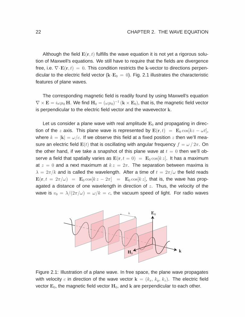
dicular to the electric field vector (k·E0 = 0). Fig. 2.1 illustrates the characteristic
features of plane waves.
The corresponding magnetic field is readily found by using Maxwell’s equation
∇× E = iωµ0 H. We find H0 = (ωµ0)−1 (k × E0), that is, the magnetic field vector
is perpendicular to the electric field vector and the wavevector k.
Let us consider a plane wave with real amplitude E0 and propagating in direc-
tion of the z axis. This plane wave is represented by E(r, t) = E0 cos[kz − ωt],
where k = |k| = ω/c. If we observe this field at a fixed position z then we’ll mea-
sure an electric field E(t) that is oscillating with angular frequency f = ω / 2π. On
the other hand, if we take a snapshot of this plane wave at t = 0 then we’ll ob-
serve a field that spatially varies as E(r, t = 0) = E0 cos[k z]. It has a maximum
at z = 0 and a next maximum at k z = 2π. The separation between maxima is
λ = 2π/k and is called the wavelength. After a time of t = 2π/ω the field reads
E(r, t = 2π/ω) = E0 cos[k z − 2π] = E0 cos[k z], that is, the wave has prop-
agated a distance of one wavelength in direction of z. Thus, the velocity of the
wave is v0 = λ/(2π/ω) = ω/k = c, the vacuum speed of light. For radio waves
k
E0
H0
λ
Figure 2.1: Illustration of a plane wave. In free space, the plane wave propagates
with velocity c in direction of the wave vector k = (kx, ky, kz). The electric field
vector E0, the magnetic field vector H0, and k are perpendicular to each other.
2.1. HOMOGENEOUS SOLUTION IN FREE SPACE 23
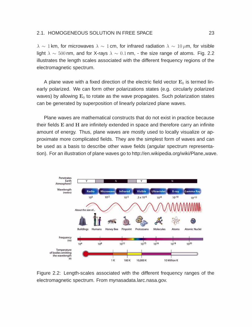
λ ∼ 1 km, for microwaves λ ∼ 1 cm, for infrared radiation λ ∼ 10µm, for visible
light λ ∼ 500 nm, and for X-rays λ ∼ 0.1 nm, - the size range of atoms. Fig. 2.2
illustrates the length scales associated with the different frequency regions of the
electromagnetic spectrum.
A plane wave with a fixed direction of the electric field vector E0 is termed lin-
early polarized. We can form other polarizations states (e.g. circularly polarized
waves) by allowing E0 to rotate as the wave propagates. Such polarization states
can be generated by superposition of linearly polarized plane waves.
Plane waves are mathematical constructs that do not exist in practice because
their fields E and H are infinitely extended in space and therefore carry an infinite
amount of energy. Thus, plane waves are mostly used to locally visualize or ap-
proximate more complicated fields. They are the simplest form of waves and can
be used as a basis to describe other wave fields (angular spectrum representa-
tion). For an illustration of plane waves go to http://en.wikipedia.org/wiki/Plane wave.
Figure 2.2: Length-scales associated with the different frequency ranges of the
electromagnetic spectrum. From mynasadata.larc.nasa.gov.

24 CHAPTER 2. THE WAVE EQUATION
2.1.2 Evanescent Waves
So far we have restricted the discussion to real kx, ky, and kz. However, this restric-
tion can be relaxed. For this purpose, let us rewrite the dispersion relation (2.14)
as
kz =√
(ω2/c2) − (k2x + k2
y) . (2.16)
If we let (k2x + k2
y) become larger than k2 = ω2/c2 then the square root no longer
yields a real value for kz. Instead, kz becomes imaginary. The solution (2.15) then
turns into
E(r, t) = ReE0 e±i(kxx+kyy)−iωt e∓|kz |z . (2.17)
These waves still oscillate like plane waves in the directions of x and y, but they
exponentially decay or grow in the direction of z. Typically, they have a plane of
origin z = const. that coincides, for example, with the surface of an insulator or
metal. If space is unbounded for z > 0 we have to reject the exponentially growing
solution on grounds of energy conservation. The remaining solution is exponen-
tially decaying and vanishes at z → ∞ (evanescere = to vanish). Because of their
exponential decay, evanescent waves only exist near sources (primary or sec-
ondary) of electromagnetic radiation. Evanescent waves form a source of stored
energy (reactive power). In light emitting devices, for example, we want to convert
k
E
kz
kx
ϕ
x
z
x
z(a) (b)
kx2+ky
2 = k2
kx
ky
plane waves
evanescent waves
(c)
Figure 2.3: (a) Representation of a plane wave propagating at an angle ϕ to the
z axis. (b) Illustration of the transverse spatial frequencies of plane waves inci-
dent from different angles. The transverse wavenumber (k2x + k2
y)1/2 depends on
the angle of incidence and is limited to the interval [0 . . . k]. (c) The transverse
wavenumbers kx, ky of plane waves are restricted to a circular area with radius
k = ω/c. Evanescent waves fill the space outside the circle.

2.1. HOMOGENEOUS SOLUTION IN FREE SPACE 25
evanescent waves into propagating waves to increase the energy efficiency.
To summarize, for a wave with a fixed (kx, ky) pair we find two different charac-
teristic solutions
Plane waves : ei [kxx + ky y] e±i |kz|z (k2x + k2
y ≤ k2)
Evanescent waves : ei [kxx + ky y] e−|kz ||z| (k2x + k2
y > k2) .(2.18)
Plane waves are oscillating functions in z and are restricted by the condition k2x +
k2y ≤ k2. On the other hand, for k2
x + k2y > k2 we encounter evanescent waves with
an exponential decay along the z-axis. Figure 2.3 shows that the larger the angle
between the k-vector and the z-axis is, the larger the oscillations in the transverse
plane will be. A plane wave propagating in the direction of z has no oscillations in
the transverse plane (k2x + k2
y =0), whereas, in the other limit, a plane wave propa-
gating at a right angle to z shows the highest spatial oscillations in the transverse
plane (k2x + k2
y = k2). Even higher spatial frequencies are covered by evanescent
waves. In principle, an infinite bandwidth of spatial frequencies (kx, ky) can be
achieved. However, the higher the spatial frequencies of an evanescent wave are,
the faster the fields decay along the z-axis will be. Therefore, practical limitations
make the bandwidth finite.
2.1.3 General Homogeneous Solution
A plane or evanescent wave characterized by the wave vector k = [kx, ky, kz] and
the angular frequency ω is only one of the many homogeneous solutions of the
wave equation. To find the general solution we need to sum over all possible plane
and evanescent waves, that is, we have to sum waves with all possible k and ω
E(r, t) = Re
∑
n,m
E0(kn, ωm) e±ikn·r−iωmt
with kn · kn = ω2m/c
2 (2.19)
The condition on the right corresponds to the dispersion relation (2.14). Further-
more, the divergence condition requires that E0(kn, ωm) · kn = 0. We have added
the argument (kn, ωm) to E0 since each plane or evanescent wave in the sum is
characterized by a different complex amplitude.

26 CHAPTER 2. THE WAVE EQUATION
The solution (2.19) assumes that there is a discrete set of frequencies and
wavevectors. Such discrete sets can be generated by boundary conditions, for
example, in a cavity where the fields on the cavity surface have to vanish. In free
space, the sum in Eq. (2.19) becomes continuous and we obtain
E(r, t) = Re
∫
k
∫
ω
E0(k, ω) e±ik·r−iωt dω d3k
with k · k = ω2/c2 (2.20)
which has the appearance of a four-dimensional Fourier transform. Notice that E0
is now a complex amplitude density, that is, amplitude per unit frequency and unit
wave vector. The difference between (2.19) and (2.20) is the same as between
Fourier series and Fourier transforms.
2.2 Spectral Representation
Let us consider solutions that are represented by a continuous distribution of fre-
quencies ω, that is, solutions of finite bandwidth. For this purpose we go back to
the complex notation (2.11) for monochromatic fields and sum (integrate) over all
monochromatic solutions
E(r, t) = Re
∞∫
−∞
E(r, ω) e−iωt dω
. (2.21)
We have replaced the complex amplitude E by E since we’re now dealing with an
amplitude per unit frequency, i.e. E = lim∆ω→0[E/∆ω]. We have also included ω in
the argument of E since each solution of constant ω has its own amplitude.
In order to eliminate the ‘Re’ sign in (2.21) we require that
E(r,−ω) = E∗(r, ω) , (2.22)
which leads us to
E(r, t) =
∫ ∞
−∞
E(r, ω) e−iωt dω (2.23)
This is simply the Fourier transform of E. In other words, E(r, t) and E(r, ω) form
a time-frequency Fourier transform pair. E(r, ω) is also denoted as the temporal

2.2. SPECTRAL REPRESENTATION 27
spectrum of E(r, t). Note that E is generally complex, while E is always real. The
inverse transform reads as
E(r, ω) =1
2π
∫ ∞
−∞
E(r, t) eiωt dt . (2.24)
Let us now replace each of the fields in Maxwell’s equations (1.32)–(1.35) by
their Fourier transforms. We then obtain
∇ · D(r, ω) = ρ(r, ω)
∇× E(r, ω) = iωB(r, ω)
∇× H(r, ω) = −iωD(r, ω) + j(r, ω)
∇ · B(r, ω) = 0
(2.25)
(2.26)
(2.27)
(2.28)
These equations are the spectral representation of Maxwell’s equations. Once a
solution for E is found, we obtain the respective time-dependent field by the inverse
transform (2.23).
2.2.1 Monochromatic Fields
A monochromatic field oscillates at a single frequency ω. According to Eq. (2.11)
it can be represented by a complex amplitude E(r) as
E(r, t) = ReE(r) e−iωt
= ReE(r) cosωt+ ImE(r) sinωt
= (1/2)[
E(r) e−iωt + E∗(r) eiωt]
. (2.29)
Inserting the last expression into Eq. (2.24) yields the temporal spectrum of a
monochromatic wave
E(r, ω′) =1
2[E(r) δ(ω′ − ω) + E∗(r) δ(ω′ + ω)] . (2.30)
Here δ(x) =∫
exp[ixt] dt/(2π) is the Dirac delta function. Iif we use Eq. (2.30)
along with similar expressions for the spectra of E, D, B, H, ρ0, and j0 in Maxwell’s

28 CHAPTER 2. THE WAVE EQUATION
equations (2.25)–(2.28) we obtain
∇ ·D(r) = ρ(r)
∇× E(r) = iωB(r)
∇× H(r) = −iωD(r) + j(r)
∇ · B(r) = 0
(2.31)
(2.32)
(2.33)
(2.34)
These equations are used whenever one deals with time-harmonic fields. They
are formally identical to the spectral representation of Maxwell’s equations (2.25)–
(2.28). Once a solution for the complex fields is found, the real time-dependent
fields are found through Eq. (2.11).
2.3 Interference of Waves
Detectors do not respond to fields, but to the intensity of fields, which is defined (in
free space) as
I(r) =
√
ε0
µ0
⟨
E(r, t) · E(r, t)⟩
, (2.35)
with 〈..〉 denoting the time-average. For a monochromatic wave, as defined in
Eq. (2.29), this expression becomes
I(r) =1
2
√
ε0
µ0|E(r)|2 . (2.36)
with |E|2 = E · E∗. The energy and intensity of electromagnetic waves will be
discussed later in Chapter 5. Using Eq. (2.15), the intensity of a plane wave turns
out to be |E0|2 since kx, ky, and kz are all real. For an evanescent wave, however,
we obtain
I(r) =1
2
√
ε0
µ0
|E0|2 e−2 kz z , (2.37)
that is, the intensity decays exponentially in z-direction. The 1/e decay length is
Lz = 1/(2kz) and characterizes the confinement of the evanescent wave.

2.3. INTERFERENCE OF WAVES 29
Next, we take a look at the intensity of a pair of fields
I(r) =√
ε0/µ0
⟨
[E1(r, t) + E2(r, t)] · [E1(r, t) + E2(r, t)]⟩
] (2.38)
=√
ε0/µ0
[⟨
E1(r, t) ·E1(r, t)⟩
+⟨
E2(r, t) · E2(r, t)⟩
+ 2⟨
E1(r, t) · E2(r, t)⟩]
= I1(r) + I2(r) + 2 I12(r)
Thus, the intensity of two fields is not simply the sum of their intensities! Instead,
there is a third term, a so-called interference term. But what about energy con-
servation? How can the combined power be larger than the sum of the individual
power contributions? It turns out that I12 can be positive or negative. Furthermore,
I12 has a directional dependence, that is, there are directions for which I12 is pos-
itive and other directions for which it is negative. Integrated over all directions, I12cancels and energy conservation is restored.
Coherent Fields
Coherence is a term that refers to how similar two fields are, both in time and
space. Coherence theory is a field on its own and we won’t dig too deep here.
Maximum coherence between two fields is obtained if the fields are monochro-
matic, their frequencies are the same, and if the two fields have a well-defined
phase relationship. Let’s have a look at the sum of two plane waves of the same
frequency ω
E(r, t) = Re[
E1 eik1·r + E2 eik2·r]
e−iωt , (2.39)
E1 E2
x
k2k1
α β
x
I(x)
I1+ I
2
Figure 2.4: Interference of two plane waves incident at angles α and β. Left:
Interference pattern along the x-axis for two different visibilities, 0.3 and 1. The
average intensity is I1 + I2.

30 CHAPTER 2. THE WAVE EQUATION
and let’s denote the plane defined by the vectors k1 and k2 as the (x,y) plane. Then,
k1 = (kx1, ky1, kz1) = k(sinα, cosα, 0) and k2 = (kx2, ky2, kz2) = k(− sin β, cosβ, 0)
(see Figure 2.4). We now evaluate this field along the x-axis and obtain
E(x, t) = Re[
E1 eikx sinα + E2 e−ikx sinβ]
e−iωt , (2.40)
which corresponds to the intensity
I(x) =1
2
√
ε0
µ0
∣
∣
[
E1 eikx sinα + E2 e−ikx sinβ]∣
∣
2(2.41)
= I1 + I2 +1
2
√
ε0
µ0
[
E1 · E∗2 eikx(sin α+sin β) + E∗
1 ·E2 e−ikx(sinα+sin β)]
= I1 + I2 +√
ε0/µ0 Re
E1 ·E∗2 eikx(sin α+sinβ)
.
This equation is valid for any complex vectors E1 and E2. We next assume that the
two vectors are real and that they are polarized along the z-axis. We then obtain
I(x) = I1 + I2 + 2√
I1 I2 cos[kx(sinα + sin β)] . (2.42)
The cosine term oscillates between +1 and -1. Therefore, the largest and smallest
signals are Imin = (I1 + I2) ± 2√I1 I2. To quantify the strength of interference one
defines the visibility
η =Imax − Imin
Imax + Imin
, (2.43)
which has a maximum value of η = 1 for I1 = I2. The period of the interfer-
ence fringes ∆x = λ/(sinα + sin β) decreases with α and β and is shortest for
α = β = π/2, that is, when the two waves propagate head-on against each other.
In this case, ∆x = λ/2.
Incoherent Fields
Let us now consider a situation for which no interference occurs, namely for two
plane waves with different frequencies ω1 and ω2. In this case Eq. (2.39) has to be
replaced by
E(x, t) = Re[
E1 eik1x sinα−iω1t + E2 e−ik2x sin β−iω2t]
. (2.44)

2.4. FIELDS AS COMPLEX ANALYTIC SIGNALS 31
Evaluating the intensity yields
I(x) =1
2
√
ε0
µ0
⟨
∣
∣E1 eik1x sinα−iω1t + E2 e−ik2x sinβ−iω2t∣
∣
2⟩
(2.45)
= I1 + I2 + 2√
I1 I2 Re
ei [k1 sinα+k2 sin β]x⟨
ei (ω2−ω1) t⟩
.
The expression 〈exp[i(ω2 − ω1)t]〉 is the time-average of a harmonically oscillating
function and yields a result of 0. Therefore, the interference term vanishes and the
total intensity becomes
I(x) = I1 + I2 , (2.46)
that is, there is no interference.
It has to be emphasized, that the two situations that we analyzed are extreme
cases. In practice there is no absolute coherence or incoherence. Any electromag-
netic field has a finite line width ∆ω that is spread around the center frequency ω.
In the case of lasers, ∆ω is a few MHz, determined by the spontaneous decay
rate of the atoms in the active medium. Thus, an electromagnetic field is at best
only partially coherent and its description as a monochromatic field with a single
frequency ω is an approximation.
2.4 Fields as Complex Analytic Signals
The relationship (2.22) indicates that the positive frequency region contains all
the information of the negative frequency region. If we restrict the integration in
Eq. (2.23) to positive frequencies, we obtain what is called a complex analytic
signal
E+(r, t) =
∫ ∞
0
E(r, ω) e−iωt dω , (2.47)
with the superscript ‘+’ denoting that only positive frequencies are included. Sim-
ilarly, we can define a complex analytic signal E− that accounts only for negative
frequencies. The truncation of the integration range causes E+ and E− to become
complex functions of time. Because E is real, we have [E+]∗ = E−. By taking the
Fourier transform of E+(r, t) and E−(r, t) we obtain E+(r, ω) and E−(r, ω), respec-
tively. It turns out that E+ is identical to E for ω > 0 and it is zero for negative

32 CHAPTER 2. THE WAVE EQUATION
frequencies. Similarly, E− is identical to E for ω < 0 and it is zero for positive fre-
quencies. Consequently, E = E+ + E−. In quantum mechanics, E− is associated
with the creation operator a† and E+ with the annihilation operator a.

Chapter 3
Constitutive Relations
Maxwell’s equations define the fields that are generated by currents and charges.
However, they do not describe how these currents and charges are generated.
Thus, to find a self-consistent solution for the electromagnetic field, Maxwell’s
equations must be supplemented by relations that describe the behavior of matter
under the influence of fields. These material equations are known as constitutive
relations.
The constitutive relations express the secondary sources P and M in terms of
the fields E and H, that is P = f [E] and M = f [H].1 According to Eq. (1.20) this
is equivalent to D = f [E] and B = f [E]. If we expand these relations into power
series
D = D0 +∂D
∂E
∣
∣
∣
∣
D=0
E +1
2
∂2D
∂E2
∣
∣
∣
∣
D=0
E2 + .. . (3.1)
we find that the lowest-order term depends linearly on E. In most practical situ-
ations the interaction of radiation with matter is weak and it suffices to truncate
the power series after the linear term. The nonlinear terms come into play when
the fields acting on matter become comparable to the atomic Coulomb potential.
This is the territory of strong field physics. Here we will entirely focus on the linear
properties of matter.
1In some exotic cases we can have P = f [E, H] and M = f [H, E], which are so-called bi-isotropic or bi-anisotropic materials. These are special cases and won’t be discussed here.
33

34 CHAPTER 3. CONSTITUTIVE RELATIONS
3.1 Linear Materials
The most general linear relationship between D and E can be written as
D(r, t) = ε0
∞∫
−∞
0∫
−∞
ε(r−r′, t−t′) E(r′, t′) d3r′ dt′ , (3.2)
which states that the response D at the location r and at time t not only depends
on the excitation E at r and t, but also on the excitation E in all other locations
r′ and all previous times t′. The integrals represent summations over all space
and over all previous times. For reasons of causality (no response before excita-
tion), the time integral only runs to t′ = 0. The response function ε is a tensor of
rank two. It maps a vector E onto a vector D according to Di =∑
j εijEj, where
i, j ∈ x, y, z. A material is called temporally dispersive if its response function
at time t depends on previous times. Similarly, a material is called spatially dis-
persive if its response at r depends also on other locations. A spatially dispersive
medium is also designated as a nonlocal medium.
Note that Eq. (3.2) is a convolution in space and time. Using the Fourier trans-
form with respect to both time and space, that is,
D(kx, ky, kz, ω) =1
(2π)4
∞∫
−∞
∞∫
−∞
∞∫
−∞
∞∫
−∞
D(x, y, z, t) eikxx eikyy eikzz eiωt dx dy dz dt , (3.3)
allows us to rewrite Eq. (3.2) as
D(k, ω) = ε0 ε(k, ω) E(k, ω) , (3.4)
where ε is the Fourier transform of ε. Note that the response at (k, ω) now only de-
pends on the excitation at (k, ω) and not on neighboring (k′, ω′). Thus, a nonlocal
relationship in space and time becomes a local relationship in Fourier space! This
is the reason why life often is simpler in Fourier space.
Spatial dispersion, i.e. a nonlocal response, is encountered near material sur-
faces or in objects whose size is comparable with the mean-free path of electrons.
In general, nonlocal effects are very difficult to account for. In most cases of inter-
est the effect is very weak and we can safely ignore it. Temporal dispersion, on

3.1. LINEAR MATERIALS 35
the other hand, is a widely encountered phenomenon and it is important to take it
accurately into account. Thus, we will be mostly concerned with relationships of
the sort
D(r, ω) = ε0 ε(ω) E(r, ω) , (3.5)
where ε(ω) is called the dielectric function, also called the relative electric permit-
tivity. Similarly, for the magnetic field we obtain
B(r, ω) = µ0 µ(ω) H(r, ω) , (3.6)
with µ(ω) being the relative magnetic permeability. Notice that the spectral repre-
sentation of Maxwell’s equations [ (2.25)–(2.28)] is formally identical to the com-
plex notation used for time-harmonic fields [ (2.31)–(2.34)] . Therefore, Eqs. (3.5)
and (3.6) also hold for the complex amplitudes of time-harmonic fields
D(r) = ε0ε(ω)E(r) , B(r) = µ0µ(ω)H(r) (3.7)
However, these equations generally do not hold for time-dependent fields E(r, t)!
One can use (3.7) for time-dependent fields only if dispersion can be ignored, that
is ε(ω) = ε and µ(ω) = µ. The only medium that is strictly dispersion-free is vac-
uum.
3.1.1 Electric and Magnetic Susceptibilities
The linear relationships (3.7) are often expressed in terms of the electric and mag-
netic susceptibilites χe and χm, respectively. These are defined as
P(r) = ε0χe(ω)E(r) , M(r) = χm(ω)H(r) . (3.8)
Using the relations (1.20) we find that ε = (1 + χe) and µ = (1 + χm).
3.1.2 Conductivity
The conductivity σ relates an induced conduction current jbond in a linear fashion
to an exciting field E. Similar to Eq. (3.7), this relationship can be represented as
jcond(r) = σ(ω)E(r) . (3.9)

36 CHAPTER 3. CONSTITUTIVE RELATIONS
It turns out that the conduction current is accounted for by the imaginary part of
ε(ω) as we shall show in the following.
Let us explicitly split the current density j into a source and a conduction cur-
rent density according to Eq. (1.11). Maxwell’s curl equation for the magnetic
field (2.33) then becomes
∇×H(r) = −iωD(r) + jcond(r) + j0(r) . (3.10)
We now introduce the linear relationships (3.7) and (3.9) and obtain
∇× H(r) = −iωε0ε(ω)E(r) + σ(ω)E(r) + j0(r)
= −iωε0
[
ε(ω) + iσ(ω)
ε0ω
]
E(r) + j0(r) . (3.11)
Thus, we see that the conductivity acts like the imaginary part of the electric per-
meability and that we can simply accommodate σ in ε by using a complex dielectric
function
[ε′ + iσ/(ωε0)] → ε (3.12)
where ε′ denotes the purely real polarization-induced dielectric constant. In the
complex notation one does not distinguish between conduction currents and po-
larization currents. Energy dissipation is associated with the imaginary part of the
dielectric function (ε′′) whereas energy storage is associated with its real part (ε′′).
With the new definition of ε, the wave equations for the complex fields E(r) and
H(r) in linear media are
∇× µ(ω)−1 ∇×E(r) − k20 ε(ω) E(r) = iωµ0 j0(r) , (3.13)
∇× ε(ω)−1 ∇×H(r) − k20µ(ω)H(r) = ∇× ε(ω)−1 j0(r) , (3.14)
where k0 = ω/c denotes the vacuum wavenumber. Note that these equations are
also valid for anisotropic media, i.e. if ε and µ are tensors.
If µ is isotropic then we can multiply Eq. (3.13) on both sides with µ. Fur-
thermore, if there are no sources we can drop j0 and obtain the Helmholtz equa-
tion (2.12), but with the difference that now k2 = k20 εµ, that is,
∇2E(r) + k2 E(r) = ∇2E(r) + k20 n
2E(r) = 0 (3.15)

3.1. LINEAR MATERIALS 37
where n =√εµ is called index of refraction.
Conductors
The conductivity σ is a measure for how good a conductor is. For example, quartz
has a conductivity of σSiO2 = 10−16 A / V m, and the conductivity of copper is
σAu = 108 A / V m. These values are different by 24 orders of magnitude! There
are hardly any other physical parameters with a comparable dynamic range.
The net charge density ρ inside a conductor is zero, no matter wether it trans-
ports a current or not. This seems surprising, but it directly follows from the charge
conservation (1.36) and Gauss’ law (1.32). Combining the two equations and us-
ing j = σE and D = ε0εE yields
∂
∂tρ(t) = − σ
ε0ερ(t) , (3.16)
which has the solution
ρ(t) = ρ(t = 0) e−t σ/(ε0ε) . (3.17)
Thus, any charge inside the conductor dissipates within a time of Tρ = ε0ε/σ. For
a perfect conductor, σ → ∞ and hence ρ(t) = 0. For realistic conductors with finite
σ the characteristic time is Tρ ∼ 10−19 s, which is so short that it can be neglected.
When a charge moves through a conductor it undergoes collisions with the lat-
tice. After a collision event, the charge is accelerated by the external field until
it is slowed down by the next collision. For good conductors (copper), the time
between collisions is typically in the order of τ ∼ 10−14 s. The sequence of acceler-
ation and deceleration events results in a finite velocity vd for the charge, called the
drift velocity. The current density due to a charge density moving at finite speed
is j = q vd n, where n2 is the charge density, i.e. the number of charges per unit
volume. The drift velocity vd is proportional to the driving field E and the propor-
tionality constant is called mobility µ3. Thus, σ = nqµ.
2Not to be confused with the index of refraction n.3Not to be confused with the magnetic permittivity µ.

38 CHAPTER 3. CONSTITUTIVE RELATIONS
In a good conductor the polarization current ∂P/∂t can be neglected because
it is much smaller than the conduction current j. In terms of a complex dielectric
constant ε = ε′ + iε′′ (c.f. Eq. 3.12) this implies that ε′′ ≫ |ε′|, that is, σ ≫ |ω ε0ε′|.
Evidently, the higher the frequency ω is, the more challenging it gets to fulfill this
condition. In fact, at optical frequencies, metals are no longer good conductors and
they are dominated by the polarization current. At lower frequencies, however, it
is legitimate to ignore the polarization current when dealing with good conductors.
Ignoring ∂P/∂t is equivalent to ignoring the real part of the complex dielectric
function (3.12), which implies k2 = (ω/c)2µε ≈ i (ω/c)2(µσ / ωε0). Consequently,
the Helmholtz equation (3.15) reads as
∇2E(r) + iωσµ0µ E(r) = 0 , (3.18)
and because of j = σE the same equation holds for the current density j. Note
that we’re using complex equation and that j(r, t) = Rej(r) exp[−iω t].
Let us now consider a semi-infinite conductor, as illustrated in Fig. 3.1. This
situation corresponds to a small section of a wire’s surface. The conductor has a
surface at x = 0 and transports a current j(r) in the z direction. Because of the
x
y
jz
z
Figure 3.1: Current density j = jz nz flowing along the surface of a conductor.

3.1. LINEAR MATERIALS 39
invariance in y and z we set jz(x) = A exp[B x] and insert into Eq. (3.18). Noting
that√i = (1 + i)/
√2 we obtain
jz(x) = jz(x = 0) e−(i−1) x/Ds with Ds =
√
2
σµ0µω. (3.19)
The length Ds is called the skin depth. Since |jz(x)/jz(0)| = exp[−x/Ds] it de-
scribes the penetration of fields and currents into the metal. Evidently, for a perfect
conductor (σ → ∞) the skin depth becomes Ds = 0, that is, all the current is trans-
ported on the surface of the metal. Ds also decreases with increasing frequency
ω, but eventually the result (3.19) becomes inaccurate because the polarization
current ∂P/∂t becomes stronger than the conduction current. In wires of finite
diameter the skin depth also depends on the curvature of the wire. At low frequen-
cies, the conductance of a wire scales with the cross-section of the wire, but at
high frequencies, the current is confined to the surface of the wire and hence the
conductance scales with the circumference.

40 CHAPTER 3. CONSTITUTIVE RELATIONS
Chapter 4
Material Boundaries
In many practical situations, electromagnetic radiation enters from one medium
into another. Examples are the refraction of light as it enters into water or the
absorption of sunlight by a solar cell. The boundary between different media is not
sharp. Instead, there is a transition zone defined by the length-scale of nonlocal
effects, usually in the size range of a few atoms, that is 0.5− 1 nm. If we don’t care
how the fields behave on this scale we can safely describe the transition from one
medium to another by a discontinuous material function. For example, at optical
frequencies the dielectric function across a glass-air interface at z = 0 can be
approximated as
ε(z) =
2.3 (z < 0) glass
1 (z > 0) air
4.1 Piecewise Homogeneous Media
Piecewise homogeneous materials consist of regions in which the material pa-
rameters are independent of position r. In principle, a piecewise homogeneous
medium is inhomogeneous and the solution can be derived from Eqs. (3.13) and
(3.14). However, the inhomogeneities are entirely confined to the boundaries and
it is convenient to formulate the solution for each region separately. These solu-
tions must be connected with each other via the interfaces to form the solution
for all space. Let the interface between two homogeneous regions Di and Dj be
denoted as ∂Dij . If εi and µi designate the constant material parameters in region
41

42 CHAPTER 4. MATERIAL BOUNDARIES
Di, the wave equations in that domain read as
(∇2 + k2i )Ei = −iωµ0µi ji +
∇ρi
ε0 εi, (4.1)
(∇2 + k2i )Hi = −∇× ji , (4.2)
where ki = (ω/c)√µiεi = k0ni is the wavenumber and ji, ρi the sources in region
Di. To obtain these equations, the identity ∇×∇× = −∇2 + ∇∇· was used and
Maxwell’s equation (1.32) was applied. Equations (4.1) and (4.2) are also denoted
as the inhomogeneous vector Helmholtz equations. In most practical applications,
such as scattering problems, there are no source currents or charges present and
the Helmholtz equations are homogeneous, that is, the terms on the right hand
side vanish.
4.2 Boundary Conditions
Eqs. (4.1) and (4.2) are only valid in the interior of the regions Di. However,
Maxwell’s equations must also hold on the boundaries ∂Dij . Due to the mate-
rial discontinuity at the boundary between two regions it is difficult to apply the
differential forms of Maxwell’s equations. We will therefore use the corresponding
integral forms (1.16) - (1.19). If we look at a sufficiently small section of the ma-
terial boundary we can approximate the boundary as being flat and the fields as
homogeneous on both sides (Fig. 4.1).
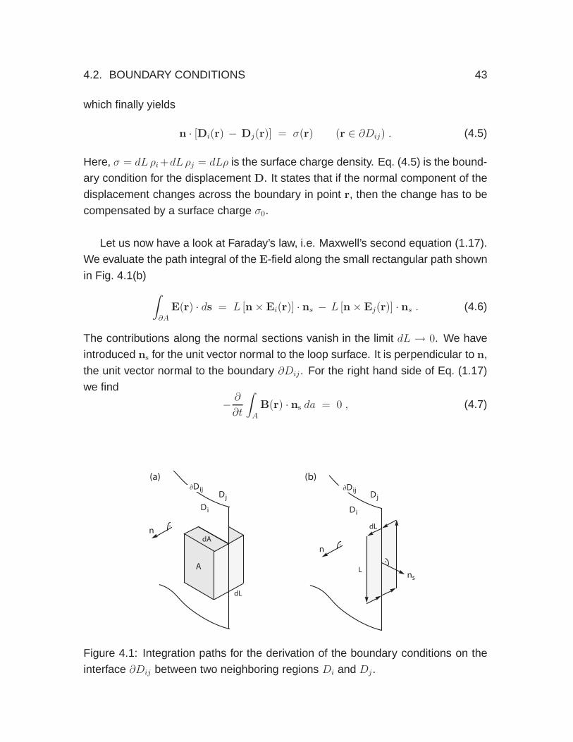
Let us first analyze Maxwell’s first equation (1.16) by considering the infinites-
imal rectangular pillbox illustrated in Fig. 4.1(a). Assuming that the fields are ho-
mogeneous on both sides, the surface integral of D becomes∫
∂V
D(r) · n da = A [n · Di(r)] − A [n · Dj(r)] , (4.3)
where A is the top surface of the pillbox. The contributions of the sides dA dis-
appear if we shrink the thickness dL of the pillbox to zero. The right hand side of
Eq. (1.16) becomes∫
V
ρ(r, t) dV = AdLρi(r) + AdLρj(r) , (4.4)
4.2. BOUNDARY CONDITIONS 43
which finally yields
n · [Di(r) − Dj(r)] = σ(r) (r ∈ ∂Dij) . (4.5)
Here, σ = dL ρi +dL ρj = dLρ is the surface charge density. Eq. (4.5) is the bound-
ary condition for the displacement D. It states that if the normal component of the
displacement changes across the boundary in point r, then the change has to be
compensated by a surface charge σ0.
Let us now have a look at Faraday’s law, i.e. Maxwell’s second equation (1.17).
We evaluate the path integral of the E-field along the small rectangular path shown
in Fig. 4.1(b)∫
∂A
E(r) · ds = L [n× Ei(r)] · ns − L [n ×Ej(r)] · ns . (4.6)
The contributions along the normal sections vanish in the limit dL → 0. We have
introduced ns for the unit vector normal to the loop surface. It is perpendicular to n,
the unit vector normal to the boundary ∂Dij . For the right hand side of Eq. (1.17)
we find
− ∂
∂t
∫
A
B(r) · ns da = 0 , (4.7)
.n
∂D ij
D i
Dj
.n
∂D ij
Di
Dj
(b)(a)
L
dL
A
dA
dL
.
ns
Figure 4.1: Integration paths for the derivation of the boundary conditions on the
interface ∂Dij between two neighboring regions Di and Dj .

44 CHAPTER 4. MATERIAL BOUNDARIES
that is, the flux of the magnetic field vanishes as the area is reduced to zero.
Combining the last two equations we arrive at
n × [Ei(r) − Ej(r)] = 0 (r ∈ ∂Dij) . (4.8)
We obtain a similar result for the Ampere-Maxwell law (1.18), with the exception
that the flux of the current density does not vanish necessarily. If we allow for the
existence of a current density that is confined to a surface layer of infinitesimal
thickness then∫
A
j(r) · ns da = LdL [ji(r) · ns] + LdL [jj(r) · ns] . (4.9)
Using an equation similar to (4.6) for H and inserting into Eq. (1.18) yields
n× [Hi(r) − Hj(r)] = K(r) (r ∈ ∂Dij) , (4.10)
where K = dL ji + dL jj = dL j being the surface current density. The fourth
Maxwell equation (1.19) yields a boundary condition similar to Eq. (4.5), but with
no surface charge, that is n·[Bi −Bj] = 0.
Taken all equations together we obtain
n · [Bi(r) − Bj(r)] = 0 (r ∈ ∂Dij)
n · [Di(r)−Dj(r)] = σ(r) (r ∈ ∂Dij)
n× [Ei(r) −Ej(r)] = 0 (r ∈ ∂Dij)
n× [Hi(r)−Hj(r)] = K(r) (r ∈ ∂Dij)
(4.11)
(4.12)
(4.13)
(4.14)
The surface charge density σ and the surface current density K are confined to
the very interface between the regions Di and Dj. Such confinement is not found
in practice and hence, σ and K are mostly of theoretical significance. The exis-
tence of σ and K demands materials that perfectly screen any charges, such as a
metal with infinite conductivity. Such perfect conductors are often used in theoret-
ical models, but they are approximations for real behavior. In most cases we can
set σ = 0 and K = 0. Any currents and charges confined to the boundary Dij are
adequately accounted for by the imaginary part of the dielectric functions εi and εj .
Note that Eq. (4.13) and (4.14) yield two equations each since the tangent
of a boundary is defined by two vector components. Thus, the boundary condi-
tions (4.11)–(4.14) constitute a total of six equations. However, these six equations

4.3. REFLECTION AND REFRACTION AT PLANE INTERFACES 45
are not independent of each other since the fields on both sides of ∂Dij are linked
by Maxwell’s equations. It can be easily shown, for example, that the conditions for
the normal components are automatically satisfied if the boundary conditions for
the tangential components hold everywhere on the boundary and Maxwell’s equa-
tions are fulfilled in both regions.
If we express each field vector Q ∈ [E, D, B, H] in terms of a vector normal to
the surface and vector parallel to the surface according to
Q = Q‖ +Q⊥n , (4.15)
and we assume the we can ignore surface charges and currents (σ = 0 and K =
0), we can represent Eqs. (4.11)-(4.14) as
B⊥i = B⊥
j on ∂Dij
D⊥i = D⊥
j on ∂Dij
E‖i = E
‖j on ∂Dij
H‖i = H
‖j on ∂Dij
(4.16)
(4.17)
(4.18)
(4.19)
4.3 Reflection and Refraction at Plane Interfaces
Applying the boundary conditions to a plane wave incident on a plane interface
leads to so-called Fresnel reflection and transmission coefficients. These coef-
ficients depend on the angle of incidence θi and the polarization of the incident
wave, that is, the orientation of the electric field vector relative to the surface.
Let us consider a linearly polarized plane wave
E1(r, t) = ReE1 eik1·r−iωt , (4.20)
as derived in Section 2.1.1. This plane wave is incident on a an interface at z = 0
(see Fig. 4.2) between two linear media characterized by ε1, µ1 and ε2, µ2, respec-
tively. The magnitude of the wavevector k1 = [kx1, ky1, kz1 ] is defined by
|k1| = k1 =ω
c
√ε1 µ1 = k0n1 , (4.21)

46 CHAPTER 4. MATERIAL BOUNDARIES
The index ‘1’ specifies the medium in which the plane wave is defined. At the inter-
face z = 0 the incident wave gives rise to induced polarization and magnetization
currents. These secondary sources give rise to new fields, that is, to transmitted
and reflected fields. Because of the translational invariance along the interface
we will look for reflected/transmitted fields that have the same form as the incident
field
E1r(r, t) = ReE1r eik1r ·r−iωt E2(r, t) = ReE2 eik2·r−iωt , (4.22)
where the first field is valid for z < 0 and the second one for z > 0. The two new
wavevectors are defined as k1r = [kx1r , ky1r , kz1r ] and k1r = [kx2, ky2, kz2 ], respec-
tively. All fields have the same frequency ω because the media are assumed to be
linear.
At z = 0, any of the boundary conditions (4.16)–(4.19) will lead to equations of
the form
A ei(kx1x+ky1y) + B ei(kx1r x+ky1r y) = C ei(kx2x+ky2y) , (4.23)
which has to be satisfied for all x and y along the boundary. This can only be
fulfilled if the periodicities of the fields are equal on both sides of the interface, that
is, kx1 = kx1r = kx2 and ky1 = ky1r = ky2. Thus, the transverse components of
the wavevector k‖ = (kx, ky) are conserved. Furthermore, E1 and E1r are defined
in the same medium (z < 0) and hence |k1|2 = |k1r|2 = k21 = k2
0 n21. Taken these
conditions together we find kz1r = ±kz1. Here, we will have to take the minus sign
E1r
(s)
a) z
k1r
E1
(s)
k1
1
E2
(s)
k2
1 1
2 2
E1r
(p)
b) z
k1rE1
(p)
k11
E2
(p)
k2
1 1
2 2
1 1
θ2θ2x x
Figure 4.2: Reflection and refraction of a plane wave at a plane interface. (a)
s-polarization, and (b) p-polarization.

4.3. REFLECTION AND REFRACTION AT PLANE INTERFACES 47
since the reflected field is propagating away from the interface. To summarize, the
three waves (incident, reflected, transmitted) can be represented as
E1(r, t) = ReE1 ei(kxx+kyy+kz1z−ωt) (4.24)
E1r(r, t) = ReE1r ei(kxx+kyy−kz1z−ωt) (4.25)
E2(r, t) = ReE2 ei(kxx+kyy+kz2z−ωt) (4.26)
The magnitudes of the longitudinal wavenumbers are given by
kz1 =√
k21 − (k2
x + k2y), kz2 =
√
k22 − (k2
x + k2y). (4.27)
Since the transverse wavenumber k‖ = [k2x + k2
y]1/2 is defined by the angle of
incidence θ1 as
k‖ =√
k2x + k2
y = k1 sin θ1 , (4.28)
it follows from (4.27) that also kz1 and kz2 can be expressed in terms of θ1.
If we denote the angle of propagation of the refracted wave as θ2 (see Fig. 4.2),
then the requirement that k‖ be continuous across the interface leads to k‖ =
k1 sin θ1 = k2 sin θ2. In other words,
n1 sin θ1 = n2 sin θ2 (4.29)
which is the celebrated Snell’s law, discovered experimentally by Willebrord Snell
around 1621. Furthermore, because kz1r = −kz1 we find that the angle of reflection
is the same as the angle of incidence (θ1r = θ1).
4.3.1 s- and p-polarized Waves
The incident plane wave can be written as the superposition of two orthogonally
polarized plane waves. It is convenient to choose these polarizations parallel and
perpendicular to the plane of incidence as
E1 = E(s)1 + E
(p)1 . (4.30)
E(s)1 is parallel to the interface, while E
(p)1 is perpendicular to the wavevector k1 and
E(s)1 . The indices (s) and (p) stand for the German “senkrecht” (perpendicular) and

48 CHAPTER 4. MATERIAL BOUNDARIES
“parallel” (parallel), respectively, and refer to the plane of incidence. Upon reflec-
tion or transmission at the interface, the polarizations (s) and (p) are conserved,
which is a consequence of the boundary condition (4.18).
s-Polarization
For s-polarization, the electric field vectors are parallel to the interface. Expressed
in terms of the coordinate system shown in Fig. 4.2 they can be expressed as
E1 =
0
E(s)1
0
E1r =
0
E(s)1r
0
E2 =
0
E(s)2
0
, (4.31)
where the superscript (s) stands for s-polarization. The magnetic field is defined
through Faraday’s law (2.32) as H = (ωµ0µ)−1 [k × E], where we assumed linear
and isotropic material properties (B = µ0µH). Using the electric field vectors (4.31)
we find
H1 =1
Z1
−(kz1/k1)E(s)1
0
(kx/k1)E(s)1
H1r =
1
Z1
(kz1/k1)E(s)1r
0
(kx/k1)E(s)1r
H2 =1
Z2
−(kz2/k2)E(s)2
0
(kx/k2)E(s)2
, (4.32)
where we have introduced the wave impedance
Zi =
√
µ0 µi
ε0 εi
(4.33)
In vacuum, µi = εi = 1 and Zi ∼ 377 Ω. It is straightforward to show that the
electric and magnetic fields are divergence free, i.e. ∇·E = 0 and ∇·H = 0.
These conditions restrict the k-vector to directions perpendicular to the field vec-
tors (k·E = k·H = 0).
4.3. REFLECTION AND REFRACTION AT PLANE INTERFACES 49
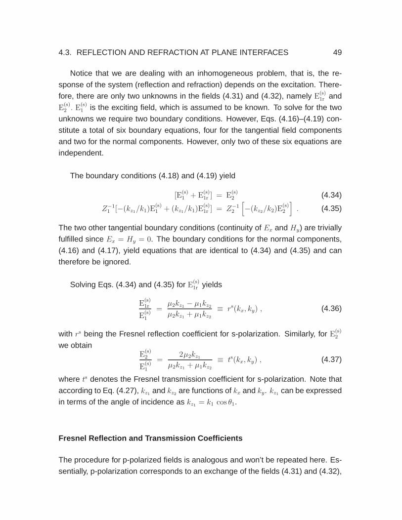
Notice that we are dealing with an inhomogeneous problem, that is, the re-
sponse of the system (reflection and refraction) depends on the excitation. There-
fore, there are only two unknowns in the fields (4.31) and (4.32), namely E(s)1r and
E(s)2 . E
(s)1 is the exciting field, which is assumed to be known. To solve for the two
unknowns we require two boundary conditions. However, Eqs. (4.16)–(4.19) con-
stitute a total of six boundary equations, four for the tangential field components
and two for the normal components. However, only two of these six equations are
independent.
The boundary conditions (4.18) and (4.19) yield
[E(s)1 + E
(s)1r ] = E
(s)2 (4.34)
Z−11 [−(kz1/k1)E
(s)1 + (kz1/k1)E
(s)1r ] = Z−1
2
[
−(kz2/k2)E(s)2
]
. (4.35)
The two other tangential boundary conditions (continuity of Ex and Hy) are trivially
fulfilled since Ex = Hy = 0. The boundary conditions for the normal components,
(4.16) and (4.17), yield equations that are identical to (4.34) and (4.35) and can
therefore be ignored.
Solving Eqs. (4.34) and (4.35) for E(s)1r yields
E(s)1r
E(s)1
=µ2kz1 − µ1kz2
µ2kz1 + µ1kz2
≡ rs(kx, ky) , (4.36)
with rs being the Fresnel reflection coefficient for s-polarization. Similarly, for E(s)2
we obtainE
(s)2
E(s)1
=2µ2kz1
µ2kz1 + µ1kz2
≡ ts(kx, ky) , (4.37)
where ts denotes the Fresnel transmission coefficient for s-polarization. Note that
according to Eq. (4.27), kz1 and kz2 are functions of kx and ky. kz1 can be expressed
in terms of the angle of incidence as kz1 = k1 cos θ1.
Fresnel Reflection and Transmission Coefficients
The procedure for p-polarized fields is analogous and won’t be repeated here. Es-
sentially, p-polarization corresponds to an exchange of the fields (4.31) and (4.32),

50 CHAPTER 4. MATERIAL BOUNDARIES
that is, the p-polarized electric field assumes the form of Eq. (4.32) and the p-
polarized magnetic field the form of Eq. (4.31).The amplitudes of the reflected and
transmitted waves can be represented as
E(p)1r = E
(p)1 rp(kx, ky) E
(p)2 = E
(p)1 tp(kx, ky) , (4.38)
where rs and tp are the Fresnel reflection and transmission coefficients for p-
polarization, respectively. In summary, for a plane wave incident on an interface
between two linear and isotropic media we obtain the following reflection and trans-
mission coefficients 1
rs(kx, ky) =µ2kz1 − µ1kz2
µ2kz1 + µ1kz2
rp(kx, ky) =ε2kz1 − ε1kz2
ε2kz1 + ε1kz2
ts(kx, ky) =2µ2kz1
µ2kz1 + µ1kz2
tp(kx, ky) =2ε2kz1
ε2kz1 + ε1kz2
√
µ2ε1
µ1ε2
(4.39)
(4.40)
The sign of the Fresnel coefficients depends on the definition of the electric field
vectors shown in Fig. 4.2. For a plane wave at normal incidence (θ1 = 0), rs and
rp differ by a factor of −1. Notice that the transmitted waves can be either plane
waves or evanescent waves. This aspect will be discussed in Chapter 4.4.
The Fresnel reflection and transmission coefficients have many interesting pre-
dictions. For example, if a plane wave is incident on a glass-air interface (incident
from the optically denser medium, i. e. glass) then the incident field can be to-
tally reflected if it is incident at an angle θ1 that is larger than a critical angle θc.
In this case, one speaks of total internal reflection. Also, there are situations for
which the entire field is transmitted. According to Eqs. (4.39), for p-polarization
this occurs when ε2kz1 = ε1kz2 . Using kz1 = k1 cos θ1 and Snell’s law (4.29) we ob-
tain kz2 = k2 [1 − (n1/n2)2 sin2 θ1]
1/2. At optical frequencies, most materials are not
magnetic (µ1 = µ2 = 1), which yields tan θ1 = n2/n1. For a glass-air interface this
occurs for θ1 ≈ 57. For s-polarization one cannot find such a condition. There-
fore, reflections from surfaces at oblique angles are mostly s-polarized. Polarizing
sunglasses exploit this fact in order to reduce glare. The Fresnel coefficients give
1For symmetry reasons, some textbooks omit the square root term in the coefficient tp. In thiscase, tp refers to the ratio of transmitted and incident magnetic field.

4.4. EVANESCENT FIELDS 51
rise to even more phenomena if we allow for two or more interfaces. Examples are
Fabry-Perot resonances and waveguiding along the interfaces.
4.4 Evanescent Fields
As already discussed in Section 2.1.2, evanescent fields can be described by plane
waves of the form Eei(kr−ωt). They are characterized by the fact that at least one
component of the wavevector k describing the direction of propagation is imagi-
nary. In the spatial direction defined by the imaginary component of k the wave
does not propagate but rather decays exponentially.
Evanescent waves never occur in a homogeneous medium but are inevitably
connected to the interaction of light with inhomogeneities, such as a plane inter-
face. Let us consider a plane wave impinging on such a flat interface between two
media characterized by optical constants ε1, µ1 and ε2, µ2. As discussed in Sec-
tion 4.3, the presence of the interface will lead to a reflected wave and a refracted
wave whose amplitudes and directions are described by Fresnel coefficients and
by Snell’s law, respectively.
To derive the evanescent wave generated by total internal reflection at the sur-
face of a dielectric medium, we refer to the configuration shown in Fig. 4.2. We
choose the x-axis to be in the plane of incidence. Using the symbols defined in
Section 4.3, the complex transmitted field vector can be expressed as
E2 =
−E(p)1 tp(kx) kz2/k2
E(s)1 ts(kx)
E(p)1 tp(kx) kx/k2
eikxx + ikz2z, (4.41)
which can be expressed entirely by the angle of incidence θ1 using kx = k1 sin θ1.
Note that we suppressed the harmonic time factor exp(−iωt). With this substitution
the longitudinal wavenumbers can be written as (cf. Eq. (4.27))
kz1 = k1
√
1 − sin2 θ1, kz2 = k2
√
1 − n2 sin2 θ1, (4.42)
where we introduced the relative index of refraction
n =
√ε1µ1√ε2µ2
. (4.43)

52 CHAPTER 4. MATERIAL BOUNDARIES
For n > 1, with increasing θ1 the argument of the square root in the expression
of kz2 gets smaller and smaller and eventually becomes negative. The critical angle
θc can be defined by the condition[
1 − n2 sin2 θ1]
= 0 , (4.44)
which describes a refracted plane wave with zero wavevector component in the
z-direction (kz2 = 0). Consequently, the refracted plane wave travels parallel to the
interface. Solving for θ1 yields
θc = arcsin[1/n] . (4.45)
For a glass/air interface at optical frequencies, we have ε2 = 1, ε1 = 2.25, and
µ1 = µ2 = 1 yielding a critical angle θc = 41.8.
For θ1 > θc, kz2 becomes imaginary. Expressing the transmitted field as a
function of the angle of incidence θ1 results in
E2 =
−iE(p)1 tp(θ1)
√
n2 sin2 θ1 − 1
E(s)1 ts(θ1)
E(p)1 tp(θ1) n sin θ1
ei sin θ1k1x e−γz , (4.46)
where the decay constant γ is defined by
γ = k2
√
n2 sin2 θ1 − 1 . (4.47)
Figure 4.3: Excitation of an evanescent wave by total internal reflection. (a) An
evanescent wave is created in a medium if the plane wave is incident at an angle
θ1 > θc. (b) Actual experimental realization using a prism and a weakly focused
Gaussian beam.

4.4. EVANESCENT FIELDS 53
This equation describes a field that propagates along the surface but decays ex-
ponentially into the medium of transmittance. Thus, a plane wave incident at an
angle θ1 > θc creates an evanescent wave. Excitation of an evanescent wave with
a plane wave at supercritical incidence (θ1 > θc) is referred to as total internal
reflection (TIR). For the glass/air interface considered above and an angle of in-
cidence of θi = 45, the decay constant is γ = 2.22/λ. This means that already
at a distance of ≈λ/2 from the interface, the time-averaged field is a factor of e
smaller than at the interface. At a distance of ≈2λ the field becomes negligible.
The larger the angle of incidence θi the faster the decay will be. Note that the Fres-
nel coefficients depend on θ1. For θ1 > θc they become complex numbers and,
consequently, the phase of the reflected and transmitted wave is shifted relative to
the incident wave. This phase shift is the origin of the so-called Goos–Hanchen
shift. Furthermore, for p-polarized excitation, it results in elliptic polarization of the
evanescent wave with the field vector rotating in the plane of incidence.
Figure 4.4: Spatial modulation of the standing evanescent wave along the propa-
gation direction of two interfering waves (x-axis) and the decay of the intensity in
the z-direction. The ordinate represents the measured optical power. From Appl.
Opt. 33, 7995 (1994).

54 CHAPTER 4. MATERIAL BOUNDARIES
Evanescent fields as described by Eq. (4.46) can be produced by directing a
beam of light into a glass prism as sketched in Fig. 4.3(b). Experimental verifica-
tion for the existence of this rapidly decaying field in the optical regime relies on
approaching a transparent body to within less than λ/2 of the interface that sup-
ports the evanescent field (c.f. Fig. 4.4).
For p- and s-polarized evanescent waves, the intensity of the evanescent wave
can be larger than that of the input beam. To see this we set z = 0 in Eq. (4.46)
and we write for an s- and p-polarized plane wave separately the intensity ratio
|E2(z = 0)|2/|E1(z = 0)|2. This ratio is equal to the absolute square of the Fresnel
transmission coefficient tp,s. These transmission coefficients are plotted in Fig. 4.5
for the example of a glass/air interface. For p-(s-)polarized light the transmitted
evanescent intensity is up to a factor of 9 (4) larger than the incoming intensity.
The maximum enhancement is found at the critical angle of TIR. The physical rea-
son for this enhancement is a surface polarization that is induced by the incoming
plane wave which is also represented by the boundary condition (4.17). A similar
enhancement effect, but a much stronger one, can be obtained when the glass/air
interface is covered by a thin layer of a noble metal. Here, so called surface plas-
mon polaritons can be excited.
0200 40 60 80
p
s
|t| (z
=0)
p,s
2
angle of incidence [ ]o
2
4
6
8
1
Figure 4.5: Intensity enhancement on top of a glass surface irradiated by a plane
wave with variable angle of incidence θ1. For p- and s-polarized waves, the en-
hancement peaks at the critical angle θc = 41.8 marked by the dotted line.
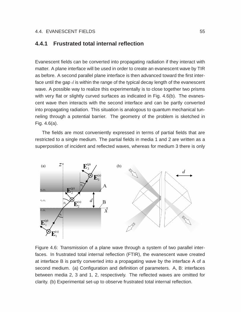
4.4. EVANESCENT FIELDS 55
4.4.1 Frustrated total internal reflection
Evanescent fields can be converted into propagating radiation if they interact with
matter. A plane interface will be used in order to create an evanescent wave by TIR
as before. A second parallel plane interface is then advanced toward the first inter-
face until the gap d is within the range of the typical decay length of the evanescent
wave. A possible way to realize this experimentally is to close together two prisms
with very flat or slightly curved surfaces as indicated in Fig. 4.6(b). The evanes-
cent wave then interacts with the second interface and can be partly converted
into propagating radiation. This situation is analogous to quantum mechanical tun-
neling through a potential barrier. The geometry of the problem is sketched in
Fig. 4.6(a).
The fields are most conveniently expressed in terms of partial fields that are
restricted to a single medium. The partial fields in media 1 and 2 are written as a
superposition of incident and reflected waves, whereas for medium 3 there is only
Figure 4.6: Transmission of a plane wave through a system of two parallel inter-
faces. In frustrated total internal reflection (FTIR), the evanescent wave created
at interface B is partly converted into a propagating wave by the interface A of a
second medium. (a) Configuration and definition of parameters. A, B: interfaces
between media 2, 3 and 1, 2, respectively. The reflected waves are omitted for
clarity. (b) Experimental set-up to observe frustrated total internal reflection.

56 CHAPTER 4. MATERIAL BOUNDARIES
a transmitted wave. The propagation character of these waves, i.e. whether they
are evanescent or propagating in either of the three media, can be determined
from the magnitude of the longitudinal wavenumber in each medium in analogy to
Eq. (4.42). The longitudinal wavenumber in medium j reads
kjz =√
k2j − k2
‖ = kj
√
1 − (k1/kj)2 sin2 θ1, j ∈ 1, 2, 3 , (4.48)
where kj = njk0 = nj(ω/c) and nj =√εjµj. In the following a layered system with
n2 < n3 < n1 will be discussed, which includes the system sketched in Fig. 4.6.
This leads to three regimes for the angle of incidence in which the transmitted
intensity as a function of the gap width d shows different behavior:
1. For θ1 < arcsin(n2/n1) or k‖ < n2k0, the field is entirely described by propa-
gating plane waves. The intensity transmitted to a detector far away from the
second interface (far-field) will not vary substantially with gapwidth, but will
only show rather weak interference undulations.
2. For arcsin(n2/n1) < θ1 < arcsin(n3/n1) or n2k0 < k‖ < n3k0 the partial field
in medium 2 is evanescent, but in medium (3) it is propagating. At the sec-
ond interface evanescent waves are converted into propagating waves. The
intensity transmitted to a remote detector will decrease strongly with increas-
ing gapwidth. This situation is referred to as frustrated total internal reflection
(FTIR).
3. For θ1 > arcsin (n3/n1) or k‖ > n3k0 the waves in layer (2) and in layer (3)
are evanescent and no intensity will be transmitted to a remote detector in
medium (3).
If we chose θ1 such that case 2 is realized (FTIR), the transmitted intensity I(d)
will reflect the steep distance dependence of the evanescent wave(s) in medium
2. However, as shown in Fig. 4.7, I(d) deviates from a purely exponential behavior
because the field in medium 2 is a superposition of two evanescent waves of the
form
c1 e−γz + c2 e+γz . (4.49)
The second term originates from the reflection of the primary evanescent wave
(first term) at the second interface and its magnitude (c2) depends on the material
properties.

4.4. EVANESCENT FIELDS 57
d/
0.2 0.4 0.6 0.8 10
0.2
0.4
0.6
0.8
1
0
transm
itte
din
tensity
(a)
(b)
(c)
Figure 4.7: Transmission of a system of three media with parallel interfaces as a
function of the gap d between the two interfaces. A p-polarized plane wave excites
the system. The material constants are n1 = 2, n2 = 1, n3 = 1.51. This leads
to critical angles θc of 30 and 49.25. For angles of incidence θi between (a) 0
and 30 the gap dependence shows interference-like behavior (here θ1 = 0, dash-
dotted line), for angles between (b) 30 and 49.25 the transmission (monotonically)
decreases with increasing gap width (here θ1 = 35, full line). (c) Intensity of the
evanescent wave in the absence of the third medium.
The discussion of FTIR in this section contains most of the ingredients ti un-
derstand the physics of optical waveguides. We will return to this topic towards the
end of this course.

58 CHAPTER 4. MATERIAL BOUNDARIES

Chapter 5
Energy and Momentum
The equations established so far describe the behavior of electric and magnetic
fields. They are a direct consequence of Maxwell’s equations and the properties
of matter. Although the electric and magnetic fields were initially postulated to
explain the forces in Coulomb’s and Ampere’s laws, Maxwell’s equations do not
provide any information about the energy content of an electromagnetic field. As
we shall see, Poynting’s theorem provides a plausible relationship between the
electromagnetic field and its energy content.
5.1 Poynting’s Theorem
If the scalar product of the field E and Eq. (1.34) is subtracted from the scalar
product of the field H and Eq. (1.33) the following equation is obtained
H · (∇× E) −E · (∇×H) = −H · ∂B∂t
− E · ∂D∂t
− j · E . (5.1)
Noting that the expression on the left is identical to ∇ · (E × H), integrating both
sides over space and applying Gauss’ theorem the equation above becomes
∫
∂V
(E× H) ·n da = −∫
V
[
H · ∂B∂t
+ E · ∂D∂t
+ j · E]
dV (5.2)
Although this equation already forms the basis of Poynting’s theorem, more insight
is provided when B and D are substituted by the generally valid equations (1.20).
59

60 CHAPTER 5. ENERGY AND MOMENTUM
Eq. (5.2) then reads as∫
∂V
(E × H) ·n da +∂
∂t
∫
V
1
2
[
D · E + B · H]
dV = −∫
V
j · E dV (5.3)
− 1
2
∫
V
[
E · ∂P∂t
−P · ∂E∂t
]
dV − µ0
2
∫
V
[
H · ∂M∂t
−M · ∂H∂t
]
dV.
This equation is a direct conclusion of Maxwell’s equations and has therefore the
same validity. Poynting’s theorem is more or less an interpretation of the equation
above. The left hand side has the general appearance of a conservation law, sim-
ilar to the conservation of charge encountered previously in Eq. (1.1).
If we set D = ε0εE and B = µ0µH then the second integrand becomes
(1/2) [ε0ε|E|2 + µ0µ|H|2], which is recognized as the sum of electric and magnetic
energy density. Thus, the second term in Eq. (5.3) corresponds to the time rate of
change of electromagnetic energy in the volume V and, accordingly, the first term
is the flux of energy in or out of V . The remaining terms on the right side are equal
to the rate of energy dissipation inside V . According to this interpretation
W =1
2
[
D ·E + B · H]
(5.4)
represents the density of electromagnetic energy, and
S = (E × H) (5.5)
is the energy flux density. S is referred to as the Poynting vector, discovered in
1883 by John Poynting and independently by Oliver Heaviside. In principle, the curl
of any vector field can be added to S without changing the conservation law (5.3),
but it is convenient to make the choice as stated in (5.5).
If the medium within V is linear and non-dispersive, the two last terms in
Eq. (5.3) equal zero and the only term accounting for energy dissipation is j · E.
To understand this term, we consider the work done per unit time on a single
charge q. In terms of the velocity v of the charge and the force F acting on it,
the work per unit time is dW/dt = F · v. Using the Lorentz force in Eq. (1) gives
dW/dt = qE · v + q [v × B] · v. Because [v × B] · v = [v × v] · B = 0 we obtain

5.1. POYNTING’S THEOREM 61
F = q v · E, which corresponds to the j · E term in Eq. (5.3).Thus, we find that the
magnetic field does no work and that it is only the electric field that gives rise to
dissipation of electromagnetic energy. The energy removed from the electromag-
netic field is transferred to the charges in matter and ultimately to other forms of
energy, such as heat.
In most practical applications we are interested in the mean value of S, that is,
the value of S averaged over several oscillation periods. This quantity describes
the net power flux density and is needed, for example, for the evaluation of radiation
patterns. Assuming that the fields are harmonic in time, linear and non-dispersive,
then the two last terms in Eq. (5.3) disappear. Furthermore, we assume that the
energy density (5.4) only accounts for polarization and magnetization currents that
a re loss-free, that is, all losses are associated with the j·E term. The time average
of Eq. (5.3) then becomes
∫
∂V
〈S(r)〉·n da = −1
2
∫
V
Re j∗(r)·E(r) dV (5.6)
where we have used complex notation. The term on the right defines the mean
energy dissipation within the volume V . 〈S〉 represents the time average of the
Poynting vector
〈S(r)〉 =1
2Re E(r) ×H∗(r) (5.7)
The magnitude of 〈S〉 is called the intensity I(r) = |〈S(r)〉|.
In the far-field, that is, far from sources and material boundaries, the electro-
magnetic field can be locally approximated by a plane wave (see Section 2.1.1).
The electric and magnetic fields are in phase, perpendicular to each other, and the
ratio of their amplitudes is constant. 〈S〉 can then be expressed by the electric field
alone as
〈S(r)〉 =1
2
1
Zi|E(r)|2 nr =
1
2
√
ε0
µ0ni |E(r)|2 (5.8)
where nr represents the unit vector in radial direction, ni =√εi µi is the index of
refraction, and Zi is the wave impedance (4.33).

62 CHAPTER 5. ENERGY AND MOMENTUM
The surface integral of 〈S〉 correspond to the total power generated or dissi-
pated inside the enclosed surface, that is,
P =
∫
∂V
〈S(r)〉·n da =
∫
∂V
I(r) da (5.9)
5.1.1 Example: Energy Transport by Evanescent Waves
Let us consider a single dielectric interface that is irradiated by a plane wave under
conditions of total internal reflection (TIR) (c.f. Section 4.4). For non-absorbing
media and for supercritical incidence, all the power of the incident wave is reflected.
One can anticipate that because no losses occur upon reflection at the interface
there is no net energy transport into the medium of transmittance. In order to
prove this fact we have to investigate the time-averaged energy flux across a plane
parallel to the interface. This can be done by considering the z-component of the
Poynting vector (cf. Eq. (5.7))
〈S〉z =1
2Re
(
ExH∗y − EyH
∗x
)
, (5.10)
where all fields are evaluated in the upper medium, i.e. the medium of trans-
mittance. Applying Maxwell’s equation (2.32) to the special case of a plane or
evanescent wave, allows us to express the magnetic field in terms of the electric
field as
H =
√
ε0ε
µ0µ
[(
k
k
)
× E
]
. (5.11)
Introducing the expressions for the transmitted field components of E and H into
Eq. (5.10), it is straightforward to prove that 〈S〉z vanishes and that there is no net
energy transport in the direction normal to the interface.
On the other hand, when considering the energy transport along the interface
(〈S〉x), a non-zero result is found:
〈S〉x =1
2
√
ε2µ2
ε1µ1sin θ1
(
|ts|2∣
∣
∣E
(s)1
∣
∣
∣
2
+ |tp|2∣
∣
∣E
(p)1
∣
∣
∣
2)
e−2γz . (5.12)
Thus, an evanescent wave transports energy along the surface, in the direction of
the transverse wavevector.

5.1. POYNTING’S THEOREM 63
5.1.2 Energy density in dispersive and lossy media
The two last terms in Eq. (5.3) strictly vanish only in a linear medium with no dis-
persion and no losses. The only medium fulfilling these conditions is vacuum. For
all other media, the last two terms only vanish approximately. In this section we
consider a linear medium with a frequency-dependent and complex ε and µ.
Let us return to the Poynting theorem stated in Eq. (5.2). While the left hand
side denotes the power flowing in or out of the volume V , the right hand side
denotes the power dissipated or generated in the volume V . The three terms on
the right hand side are of similar form and so we start by considering first the
electric energy term E · (∂D/∂t). The electric energy density wE at the time t is
wE(r, t) =
∫ t
−∞
E(r, t′) · ∂D(r, t′)
∂t′dt′ . (5.13)
We now express the fields E and D in terms of their Fourier transforms as E(t′)=∫
E(ω) exp[−iωt′] dω and D(t′) =∫
D(ω) exp[−iωt′] dω, respectively. In the last ex-
pression we substitute ω = −ω′ and obtain D(t′)=∫
D∗(ω′) exp[iω′t′] dω′, where we
used D(−ω′)= D∗(ω′) since D(t) is real (c.f. Eq. (2.22)). Using the linear relation
D = ε0 εE and inserting the Fourier transforms in Eq. (5.13) yields
wE(r, t) = ε0
∫ ∞
−∞
∫ ∞
−∞
ω′ ε∗(ω′)
ω′ − ωE(ω) · E∗(ω′) ei(ω′−ω)t dω′ dω , (5.14)
where we have carried out the differentiation and integration over time and as-
sumed that the fields were zero at t→ −∞. For later purposes it is advantageous
to represent the above result in different form. Using the substitutions u′ = −ω and
u = −ω′ and making use of E(−u)= E∗(u) and ε(−u)= ε∗(u) gives an expression
similar to Eq. (5.14) but in terms of u and u′. Finally, we add this expression to
Eq. (5.14) and take one half of the resulting sum, which yields
wE(r, t) =ε0
2
∫ ∞
−∞
∫ ∞
−∞
[
ω′ε∗(ω′) − ωε(ω)
ω′ − ω
]
E(ω) · E∗(ω′) ei(ω′−ω)t dω′ dω . (5.15)
Similar expressions are obtained for the magnetic term H · (∂B/∂t) and the dissi-
pative term j ·E in Eq. (5.2).
If ε(ω) is a complex function then wE not only accounts for the energy density
built up in the medium but also for the energy transferred to the medium, such as
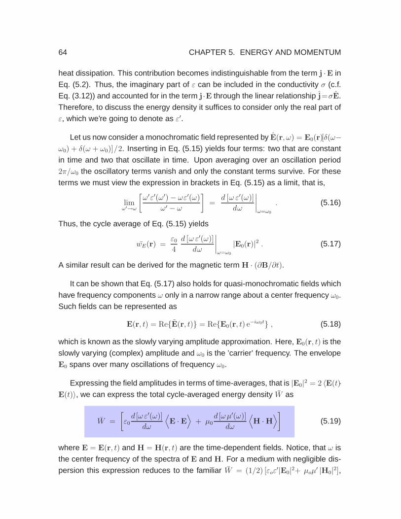
64 CHAPTER 5. ENERGY AND MOMENTUM
heat dissipation. This contribution becomes indistinguishable from the term j ·E in
Eq. (5.2). Thus, the imaginary part of ε can be included in the conductivity σ (c.f.
Eq. (3.12)) and accounted for in the term j ·E through the linear relationship j=σE.
Therefore, to discuss the energy density it suffices to consider only the real part of
ε, which we’re going to denote as ε′.
Let us now consider a monochromatic field represented by E(r, ω) = E0(r)[δ(ω−ω0) + δ(ω + ω0)]/2. Inserting in Eq. (5.15) yields four terms: two that are constant
in time and two that oscillate in time. Upon averaging over an oscillation period
2π/ω0 the oscillatory terms vanish and only the constant terms survive. For these
terms we must view the expression in brackets in Eq. (5.15) as a limit, that is,
limω′→ω
[
ω′ε′(ω′) − ωε′(ω)
ω′ − ω
]
=d [ω ε′(ω)]
dω
∣
∣
∣
∣
ω=ω0
. (5.16)
Thus, the cycle average of Eq. (5.15) yields
wE(r) =ε0
4
d [ω ε′(ω)]
dω
∣
∣
∣
∣
ω=ω0
|E0(r)|2 . (5.17)
A similar result can be derived for the magnetic term H · (∂B/∂t).
It can be shown that Eq. (5.17) also holds for quasi-monochromatic fields which
have frequency components ω only in a narrow range about a center frequency ω0.
Such fields can be represented as
E(r, t) = ReE(r, t) = ReE0(r, t) e−iω0t , (5.18)
which is known as the slowly varying amplitude approximation. Here, E0(r, t) is the
slowly varying (complex) amplitude and ω0 is the ’carrier’ frequency. The envelope
E0 spans over many oscillations of frequency ω0.
Expressing the field amplitudes in terms of time-averages, that is |E0|2 = 2 〈E(t)·E(t)〉, we can express the total cycle-averaged energy density W as
W =
[
ε0d [ωε′(ω)]
dω
⟨
E · E⟩
+ µ0d [ωµ′(ω)]
dω
⟨
H · H⟩
]
(5.19)
where E = E(r, t) and H = H(r, t) are the time-dependent fields. Notice, that ω is
the center frequency of the spectra of E and H. For a medium with negligible dis-
persion this expression reduces to the familiar W = (1/2) [εoε′|E0|2+ µoµ
′ |H0|2],

5.2. THE MAXWELL STRESS TENSOR 65
which follows from Eq. (5.4) using the dispersion-free constitutive relations. Be-
cause of d(ωε′)/dω > 0 and d(ωµ′)/dω > 0 the energy density is always positive,
even for metals with ε′ < 0.
5.2 The Maxwell Stress Tensor
In this section we use Maxwell’s equations to derive the conservation law for lin-
ear momentum in an electromagnetic field. The net force exerted on an arbitrary
object is entirely determined by Maxwell’s stress tensor. In the limiting case of an
infinitely extended object, the formalism renders the known formulas for radiation
pressure.
The general law for forces in electromagnetic fields is based on the conser-
vation law for linear momentum. To derive this conservation law we will consider
Maxwell’s equations in vacuum. In this case we have D = ε0E and B = µ0H.
Later we will relax this constraint. The conservation law for linear momentum is
entirely a consequence of Maxwell’s equations (1.16) - (1.19) and of the Lorentz
force law (5), which connects the electromagnetic world with the mechanical one.
If we operate on Maxwell’s first equation by ×ε0E, on the second equation by
×µ0H, and then add the two resulting equations we obtain
ε0(∇× E) ×E + µ0(∇× H) ×H = j× B − 1
c2
[
∂H
∂t× E
]
+1
c2
[
∂E
∂t×H
]
(5.20)
We have omitted the arguments (r, t) for the different fields and we used ε0µ0 =
1/c2. The last two expressions in Eq. (5.20) can be combined to (1/c2) d/dt [E×H].
For the first expression in Eq. (5.20) we can write
ε0(∇× E) × E = (5.21)
ε0
∂/∂x(E2x −E2/2) + ∂/∂y(ExEy) + ∂/∂z(ExEz)
∂/∂x(ExEy) + ∂/∂y(E2y −E2/2) + ∂/∂z(EyEz)
∂/∂x(ExEz) + ∂/∂y(EyEz) + ∂/∂z(E2z −E2/2)
− ε0E∇·E
= ∇ · [ε0EE − (ε0/2)E2↔
I ] − ρE .

66 CHAPTER 5. ENERGY AND MOMENTUM
where Eq. (1.32) has been used in the last step. The notation EE denotes the
outer product, E2 = E2x + E2
y + E2z is the electric field strength, and
↔
I denotes the
unit tensor. A similar expression can be derived for µ0(∇× H) × H. Using these
two expressions in Eq. (5.20) we obtain
∇· [ε0EE − µ0HH − 1
2(ε0E
2 +µ0H2)
↔
I ] =d
dt
1
c2[E×H] + ρE + j×B . (5.22)
The expression in brackets on the left hand side is called Maxwell’s stress tensor
in vacuum, usually denoted as↔
T. In Cartesian components it reads as
↔
T =
[
ε0EE− µ0HH − 1
2(ε0E
2 + µ0H2)
↔
I
]
= (5.23)
ε0(E2x −E2/2) + µ0(H
2x −H2/2) ε0ExEy + µ0HxHy
ε0ExEy + µ0HxHy ε0(E2y −E2/2) + µ0(H
2y −H2/2)
ε0ExEz + µ0HxHz ε0EyEz + µ0HyHz
ε0ExEz + µ0HxHz
ε0EyEz + µ0HyHz
ε0(E2z −E2/2) + µ0(H
2z −H2/2)
After integration of Eq. (5.22) over an arbitrary volume V which contains all sources
ρ and j we obtain∫
V
∇·↔
T dV =d
dt
1
c2
∫
V
[E × H] dV +
∫
V
[ρE + j ×B] dV . (5.24)
The last term is recognized as the mechanical force (cf. Eq. (5)). The volume inte-
gral on the left can be transformed to a surface integral using Gauss’s integration
law∫
V
∇·↔
T dV =
∫
∂V
↔
T ·n da . (5.25)
∂V denotes the surface of V , n the unit vector perpendicular to the surface, and
da an infinitesimal surface element. We then finally arrive at the conservation law
for linear momentum
∫
∂V
↔
T (r, t) · n(r) da =d
dt
[
Gfield + Gmech
]
(5.26)
Here, Gmech and Gfield denote the mechanical momentum and the field momentum,
respectively. In Eq. (5.26) we have used Newton’s expression of the mechanical

5.2. THE MAXWELL STRESS TENSOR 67
force F = d/dtGmech and the definition of the field momentum (Abraham density)
Gfield =1
c2
∫
V
[E ×H] dV (5.27)
This is the momentum carried by the electromagnetic field within the volume V . It
is created by the dynamic terms in Maxwell’s curl equations. The time-derivative
of the field momentum is zero when it is averaged over one oscillation period and
hence the average mechanical force becomes
〈F〉 =
∫
∂V
〈↔
T (r, t)〉 · n(r) da (5.28)
with 〈...〉 denoting the time average. Equation (5.28) is of general validity. It allows
the mechanical force acting on an arbitrary body within the closed surface ∂V to
be calculated (see Figure 5.1). The force is entirely determined by the electric
and magnetic fields on the surface ∂V . It is interesting to note that no material
properties enter the expression for the force; the entire information is contained
in the electromagnetic field. The only material constraint is that the body is rigid.
If the body deforms when it is subject to an electromagnetic field we have to in-
clude electrostrictive and magnetostrictive forces. Since the enclosing surface is
B
∂ V
F
incident field
scattered field
Figure 5.1: The mechanical force F acting on the object B is entirely determined
by the electric and magnetic fields at an arbitrary surface ∂V enclosing B.
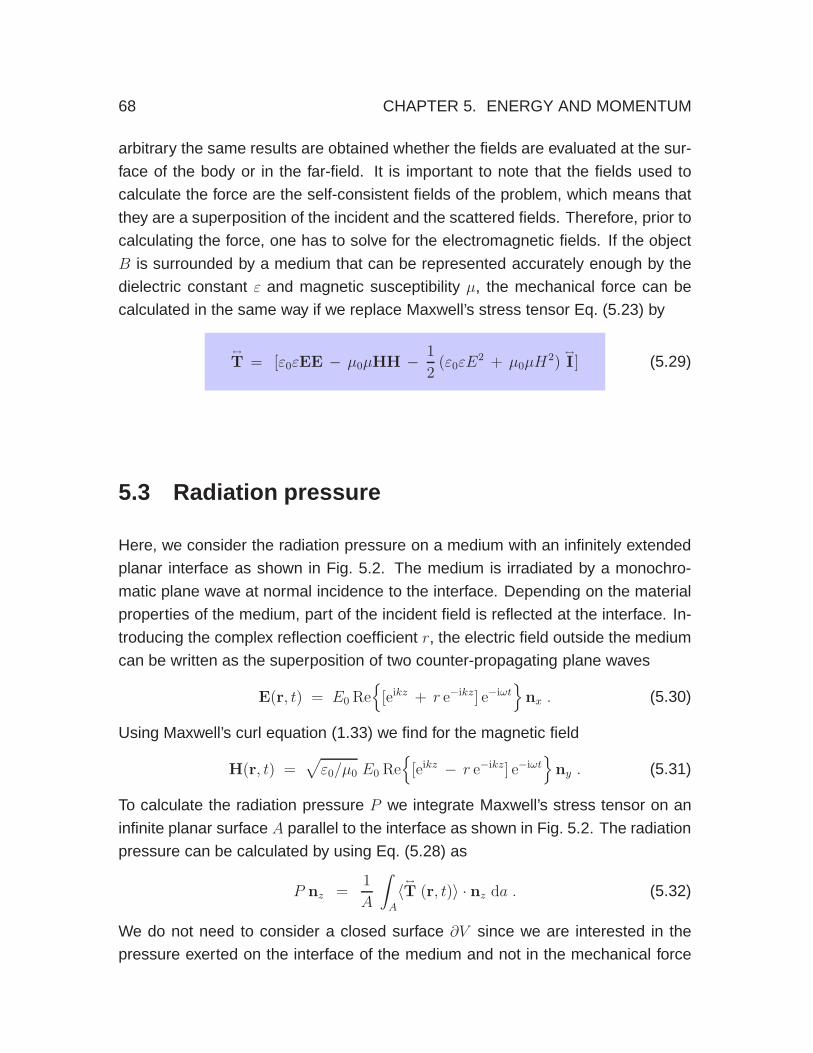
68 CHAPTER 5. ENERGY AND MOMENTUM
arbitrary the same results are obtained whether the fields are evaluated at the sur-
face of the body or in the far-field. It is important to note that the fields used to
calculate the force are the self-consistent fields of the problem, which means that
they are a superposition of the incident and the scattered fields. Therefore, prior to
calculating the force, one has to solve for the electromagnetic fields. If the object
B is surrounded by a medium that can be represented accurately enough by the
dielectric constant ε and magnetic susceptibility µ, the mechanical force can be
calculated in the same way if we replace Maxwell’s stress tensor Eq. (5.23) by
↔
T = [ε0εEE − µ0µHH − 1
2(ε0εE
2 + µ0µH2)
↔
I ] (5.29)
5.3 Radiation pressure
Here, we consider the radiation pressure on a medium with an infinitely extended
planar interface as shown in Fig. 5.2. The medium is irradiated by a monochro-
matic plane wave at normal incidence to the interface. Depending on the material
properties of the medium, part of the incident field is reflected at the interface. In-
troducing the complex reflection coefficient r, the electric field outside the medium
can be written as the superposition of two counter-propagating plane waves
E(r, t) = E0 Re
[eikz + r e−ikz] e−iωt
nx . (5.30)
Using Maxwell’s curl equation (1.33) we find for the magnetic field
H(r, t) =√
ε0/µ0 E0 Re
[eikz − r e−ikz] e−iωt
ny . (5.31)
To calculate the radiation pressure P we integrate Maxwell’s stress tensor on an
infinite planar surface A parallel to the interface as shown in Fig. 5.2. The radiation
pressure can be calculated by using Eq. (5.28) as
P nz =1
A
∫
A
〈↔
T (r, t)〉 · nz da . (5.32)
We do not need to consider a closed surface ∂V since we are interested in the
pressure exerted on the interface of the medium and not in the mechanical force

5.3. RADIATION PRESSURE 69
k
E0
A
H0
nx
ny
nz
Figure 5.2: Configuration used to derive the radiation pressure.
acting on the medium. Using the fields of Eqs. (5.30) and (5.31) we find that the
first two terms in Maxwell’s stress tensor Eq. (5.23) give no contribution to the
radiation pressure. The third term yields
〈↔
T (r, t)〉 · nz = −1
2〈ε0E
2 + µ0H2〉nz =
ε0
2E2
0 [1 + |r|2]nz . (5.33)
Using the definition of the intensity of a plane wave I0 = (ε0/2)cE20 , c being the
vacuum speed of light, we can express the radiation pressure as
P =I0c
[1 + R] , (5.34)
with R = |r|2 being the reflectivity. For a perfectly absorbing medium we have
R = 0, whereas for a perfectly reflecting medium R = 1. Therefore, the radiation
pressure on a perfectly reflecting medium is twice as high as for a perfectly ab-
sorbing medium.
To conclude this chapter we should emphasize the importance of electromag-
netic energy and momentum. Energy and momentum are fundamental concepts
of physics that make transitions between different fields feasible. For example,
electromagnetic energy can be transferred to heat, which is a concept of ther-
modynamics, and electromagnetic momentum can be transferred to mechanical

70 CHAPTER 5. ENERGY AND MOMENTUM
forces, which is a concept of classical mechanics. Electromagnetic energy and
momentum are also used in Lagrangian and Hamiltonian formalisms, which form
the stepping stones to quantum mechanics and quantum electrodynamics. Thus,
energy and momentum make it possible to transition between different fields of
physics. Such transitions cannot be accomplished by more standard electrical
concepts such as voltage and current.

Chapter 6
Radiation
In this chapter we will discuss the emission of electromagnetic radiation from ele-
mentary sources. A stationary charge yields a static electric field, but it does not
radiate. Similarly, a uniformly moving charge (a current) yields a static magnetic
field, but it does not radiate. It is the acceleration of charge that gives rise to ra-
diation. The smallest radiating unit is a dipole, an electromagnetic point source.
According to linear response theory, a point source excitation yields the system
response function, from which we can calculate the fields of more complicated
sources by using the superposition principle. The system response function is
also referred to as the Green function.
6.1 Green functions
Before calculating the fields radiated by elementary sources let us discuss an im-
portant mathematical concept, namely the concept of the Green function. Consider
the following general, inhomogeneous equation:
LA(r) = B(r) . (6.1)
L is a linear operator acting on the vectorfield A representing the unknown re-
sponse of the system. The vectorfield B is a known source function and makes
the differential equation inhomogeneous. A well-known theorem for linear differen-
tial equations states that the general solution is equal to the sum of the complete
71

72 CHAPTER 6. RADIATION
homogeneous solution (B=0) and a particular inhomogeneous solution. Here, we
assume that the homogeneous solution (A0) is known. We thus need to solve for
an arbitrary particular solution.
Usually it is difficult to find a solution of Eq. (6.1) and it is easier to consider
the special inhomogeneity δ(r−r′), which is zero everywhere, except in the point
r = r′. Then, the linear equation reads as
LGi(r, r′) = ni δ(r− r′) (i = x, y, z) , (6.2)
where ni denotes an arbitrary constant unit vector. In general, the vectorfield Gi is
dependent on the location r′ of the inhomogeneity δ(r−r′). Therefore, the vector r′
has been included in the argument of Gi. The three equations given by Eq. (6.2)
can be written in closed form as
L↔
G(r, r′) =↔
I δ(r − r′) , (6.3)
where the operator L acts on each column of↔
G separately and↔
I is the unit tensor.
The dyadic function↔
G fulfilling Eq. (6.3) is known as the dyadic Green function.
In a next step, assume that Eq. (6.3) has been solved and that↔
G is known.
Postmultiplying Eq. (6.3) with B(r′) on both sides and integrating over the volume
V in which B 6=0 gives∫
V
L↔
G(r, r′)B(r′) dV ′ =
∫
V
B(r′) δ(r− r′) dV ′ . (6.4)
The right hand side simply reduces to B(r) and with Eq. (6.1) it follows that
LA(r) =
∫
V
L↔
G(r, r′)B(r′) dV ′ . (6.5)
If on the right hand side the operator L is taken out of the integral, the solution of
Eq. (6.1) can be expressed as
A(r) =
∫
V
↔
G (r, r′)B(r′) dV ′ . (6.6)
Thus, the solution of the original equation can be found by integrating the product
of the dyadic Green function and the inhomogeneity B over the source volume V .

6.2. SCALAR AND VECTOR POTENTIALS 73
The assumption that the operators L and∫
dV ′ can be interchanged is not
strictly valid and special care must be applied if the integrand is not well behaved.
Most often↔
G is singular at r = r′ and an infinitesimal exclusion volume surround-
ing r= r′ has to be introduced. As long as we consider field points outside of the
source volume V , i.e. r 6∈V , we do not need to consider these tricky issues.
6.2 Scalar and Vector Potentials
The E and B fields define a total of six functions in space and time. It turns out, that
these fields are not independent and that one needs fewer functions to uniquely
determine the electromagnetic field. The vector potential A and the scalar po-
tential φ constitute a set of only four functions which, depending on the type of
problem, can be reduced to even fewer functions. These potentials are also of key
importance in quantum mechanics.
Let’s consider Maxwell’s equation ∇ ·B = 0 and replace B by another function.
Because, ∇ · ∇× = 0 we choose B = ∇ × A. Next, we consider Faraday’s law
∇ × E = −∂B/∂t and replace B by ∇ × A. We obtain ∇ × [E + ∂A/∂t] = 0.
Considering that ∇ × ∇ = 0, we set [E + ∂A/∂t] = −∇φ, which yields E =
−∂A/∂t −∇φ. To summarize,
E(r, t) = − ∂
∂tA(r, t) −∇φ(r, t)
B(r, t) = ∇×A(r, t)
(6.7)
(6.8)
It turns out that these definitions of vector potential A and scalar potential φ are
not unique. If the potentials are replaced by new potentials A, φ according to
A → A + ∇χ and φ→ φ− ∂χ/∂t , (6.9)
with χ(r, t) being an arbitrary gauge function, Maxwell’s equations remain unaf-
fected. This is easily seen by introducing the above substitutions in the definitions
of A and φ.

74 CHAPTER 6. RADIATION
6.2.1 The Gauges
Any vectorfield F is specified by the definition of ∇·F and ∇×F. A vectorfield with
∇ · F = 0 is called transverse, whereas ∇× F = 0 defines a longitudinal field.
So far, we have defined the curl of A, i.e. ∇ × A = B. However, we did not
specify ∇ · A. The choice of ∇ · A does not affect the fields E and B. Typically
one chooses ∇ · A such that the wave equation for A assumes a simple form
or that favorable symmetries can be exploited. To demonstrate this, we consider
Maxwell’s equation ∇ × H = ∂D/∂t + j. Using the relations (1.20) we obtain
∇× B − (1/c2)∂E/∂t = µ0[∇× M + ∂P/∂t + j], where the expression in brackets
is the total current density jtot. Inserting Eqs. (6.7) and (6.8) yields
∇×∇× A +1
c2∂2
∂t2A +
1
c2∇∂φ
∂t= µ0 jtot , (6.10)
which can be rewritten as
∇2A − 1
c2∂2
∂t2A = −µ0 jtot + ∇
[
∇ · A +1
c2∂φ
∂t
]
. (6.11)
The expression in brackets contains a ∇ · A term, which we can choose as we
wish. Finally, we also express Gauss’ law ∇·D = ρ in terms of A and φ and obtain
∇ · (∂A/∂t+ ∇φ) = −ρtot/ε0 . (6.12)
There is again a ∇ · A term that can be arbitrarily chosen.
Lorenz Gauge
In the Lorenz gauge one chooses ∇ · A = −(1/c2) ∂φ/∂t1, which yields
[
∇2 − 1
c2∂2
∂t2
]
A = −µ0 jtot
[
∇2 − 1
c2∂2
∂t2
]
φ = − 1
ε0ρtot
(6.13)
(6.14)
1This has the form of a continuity equation (A is the current density and φ/c2 is the chargedensity).

6.2. SCALAR AND VECTOR POTENTIALS 75
Thus, we obtain two decoupled partial differential equations of the same form for
A and φ. Note, that one ends up with the same differential equations by a proper
choice of the gauge function χ (6.9).
The advantage of the Lorenz gauge is that the vectorial differential equation for
A is decoupled into a set of three independent scalar differential equations, that
is, each vector component Ai depends only on the source component jtoti. There
is no mixing of components i ∈ [x, y, z].
Coulomb Gauge
In the Coulomb gauge one chooses ∇ · A = 0. This gauge is also referred to as
the transverse gauge or the minimal coupling gauge. With this choice of gauge
Eqs. (6.11) and (6.12) reduce to
[
∇2 − 1
c2∂2
∂t2
]
A = −µ0 jtot +1
c2∇∂φ
∂t
∇2 φ = − 1
ε0ρtot . (6.15)
Here, the scalar potential φ is determined by a Poisson equation, that is, there is no
retardation and φ is an instantaneous function. The Coulomb gauge is mostly used
for problems in quantum optics and is less important for this course. There are
many more gauges, which we won’t discuss here. Among them are the Poincare
gauge, the Landau gauge, and the Weyl gauge. We will be mostly dealing with the
Lorenz gauge.
Note that by going from E, H to A, φwe reduced the field parameters from six to
four (three per vector and one per scalar). It turns out that the four parameters are
still redundant and that they can be reduced even more. One way is to introduce
the so-called Hertz potential Π(r), which has only three components. The vector
and scalar potentials are related to Π as A = (1/c2) ∂Π/∂t and φ = −∇ · Π, re-
spectively. Using so-called Debye potentials is yet another representation of fields,
but these won’t be discussed here.

76 CHAPTER 6. RADIATION
6.3 Dipole Radiation
In this section we will derive the electromagnetic field of a dipole source, the small-
est radiating system. Mathematically, the dipole source corresponds to a delta
excitation, and the response to a delta excitation is the Green function discussed
previously. Any source can be thought of as being composed of individual point
sources with different origins. In other words, any macroscopic source volume can
be chopped up into little infinitesimal cubes, each of which carries a current that is
represented by a delta function.
As shown in Fig. 6.1, a dipole is a separation of a pair of charges by an in-
finitesimal distance ds = ns ds. The dipole moment p is defined as
p(t) = q(t) ds . (6.16)
The time derivative of the dipole moment is
∂
∂tp(t) =
[
∂ q(t)
∂tns
]
ds = [j da] ds = j dV , (6.17)
where [j · ns]da is the current flowing through the cross-sectional area da. The
product of da and ds defines the infinitesimal source volume dV .
Let us now consider an arbitrary macroscopic current density j(r) that is entirely
contained within the volume V . We can express this current density in terms of a
sum of microscopic point current densities. In terms of the Dirac delta function δ
+q
-q
ds da
+ρ
ns
−ρ
ds
ns
Figure 6.1: Illustration of a dipole with moment p = q ds = q dsns. Left: in terms
of discrete point charges q; Right: in terms of charge distributions ρ.

6.3. DIPOLE RADIATION 77
this sum becomes
j(r) =
∞∫
−∞
∞∫
−∞
∞∫
−∞
j(x′, y′, z′) δ(x− x′) δ(y − y′) δ(z − z′) dx′ dy′ dz′ (6.18)
=
∫
V
j(r′) δ(r − r′) dV ′ , (6.19)
Here, j(r′)δ(r − r′)dV ′ are elementary point currents. Using Eq. (6.17) we obtain
the current density of an elementary dipole source
j(r, t) =∂
∂tp(t) δ(r− r0) (6.20)
where r0 is the dipole location.
In principle, we can now determine the fields E and H radiated by a dipole p in
free space by inserting (6.20) into the wave equation (2.1). This task is, however,
easier accomplished by replacing E and H by the potentials A and φ, as discussed
previously.
6.3.1 Vector Potential of a Time-Harmonic Dipole
To calculate the fields of a dipole we will use the Lorenz gauge. The appeal of the
Lorenz gauge is its symmetry, that is, there is a scalar wave equation of the form
[∇2 − (1/c2)∂2/∂t2] Ψ = Θ for any of the field components Ax, Ay, Az, φ.
Let us start with deriving the vectorfield of a dipole with a harmonic time depen-
dence. In this case, p(t) = Rep exp[−iωt], with p being a complex amplitude.
Thus, we can use complex notation and the equations for the components of A
become[
∇2 + k2]
Ai(r) = iωµ0 pi δ(r − r′) . (6.21)
where we used Eq. (6.20) for the current density of a dipole field. Let us now define
the scalar Green function as G0 = i Ai/ωµ0 pi. Then, Eq. (6.21) turns into
[
∇2 + k2]
G0(r, r′) = −δ(r − r′) (6.22)

78 CHAPTER 6. RADIATION
We have included the origin of the the point source (r′) in the argument of G0 to
remind us where the origin of the point source is. In other words G0(r, r′) is the
response at r to to a dipole source at r′.
In free space, G0(r, r′) must be point symmetric, because the source depends
only on the radial distance R = |r − r′| and things don’t change if the coordinate
system is rotated around the origin r = r′. To solve Eq. (6.22) we will try the
following ansatz
RG0 = a1 eikR + a2 e−ikR , (6.23)
which is a superposition of an outgoing and an incoming wave. After inserting
into Eq. (6.22) and integrating on both sides over a small spherical volume ∆V
centered at R = 0 and with radius ro. We obtain∫
∆V
∇2 1
RdV + k2
∫
∆V
1
RdV =
1
a1 + a2(6.24)
The second term integrates to 2πk2r2o and the first term is calculated as
∫
∆V
∇ ·[
∇ 1
R
]
dV =
∫
∂∆V
[
∇ 1
R
]
· nR da = −∫
∂∆V
nR · nR
R2da = −4π . (6.25)
where we used Gauss’ theorem (1.28). Thus, for ro → 0 we obtain (a1 + a2) =
1 / 4π. Finally, in free-space the radiation released by the point source is not com-
ing back, which implies that we can drop the incoming wave in (6.23) or, equiva-
lently, set a2 = 0. The solution for the scalar Green function becomes
G0(r, r′) =
ei k |r−r′|
4π|r−r′| (6.26)
G0 defines the vector potential at r due to a dipole p at r′ according to
A(r) = −i ωµ0ei k |r−r
′|
4π|r−r′| p . (6.27)
What if the source is not a dipole but an arbitrary current distribution? In this case
we go back to Eq. (6.22) and multiply both sides with µ0 jtoti(r′), where jtoti
is the
i-th vector component of the total current density jtot. Integrating both sides over
the source volume V yields
µ0
∫
V
[
∇2+ k2]
G0(r, r′) jtoti
(r′) dV ′ = −µ0
∫
V
δ(r−r′) jtoti(r′) dV ′
= = −µ0 jtoti(r) , (6.28)

6.3. DIPOLE RADIATION 79
where we used the definition of the delta function. We now assume that the ob-
servation point r is outside the source volume described by the coordinate r′. In
this case, we can swap the sequence of integration and differentiation in Eq. (6.28)
and obtain[
∇2+ k2]
µ0
∫
V
G0(r, r′) jtoti
(r′) dV ′ = −µ0 jtoti(r) . (6.29)
Comparing this equation with Eq. (6.13) we conclude that
A(r) = µ0
∫
V
G0(r, r′) jtot(r
′) dV ′ (6.30)
Thus, the solution for A turns out to be the linear superposition of dipole fields with
different origins r′ and different weights jtot.
6.3.2 Electric and Magnetic Dipole Fields
Now that we have derived the vector potential A of an oscillation dipole, we find
the magnetic field using B = ∇×A and the electric field using Maxwell’s equation
E = i(ω/k2)∇× B. Skipping the details of the calculation, we find
E(r) = ω2µ0
↔
G0 (r, r′)p
H(r) = −iω[
∇×↔
G0 (r, r′)]
p
(6.31)
(6.32)
where we introduced the so-called dyadic Green function↔
G0 defined as
↔
G0 (r, r′) =
[
↔
I +1
k2∇∇
]
G0(r, r′) (6.33)
with G0 being the scalar Green function (6.26) and↔
I being the unit tensor. Notice
that↔
G0 is a tensor. It is straightforward to calculate↔
G0 in the major three coordinate
systems. In a Cartesian system↔
G0 can be written as
↔
G0 (r, r′) =exp(ikR)
4πR
[(
1 +ikR− 1
k2R2
)
↔
I +3 − 3ikR− k2R2
k2R2
RR
R2
]
(6.34)

80 CHAPTER 6. RADIATION
where R is the absolute value of the vector R = r−r′ and RR denotes the outer
product of R with itself. Equation (6.34) defines a symmetric 3×3 matrix
↔
G0 =
Gxx Gxy Gxz
Gxy Gyy Gyz
Gxz Gyz Gzz
, (6.35)
which, together with Eqs. (6.31) and (6.32), determines the electromagnetic field
of an arbitrary electric dipole p with Cartesian components px, py, pz. The tensor
[∇×↔
G0] can be expressed as
∇×↔
G0 (r, r′) =exp(ikR)
4πR
k(
R×↔
I)
R
(
i − 1
kR
)
, (6.36)
where R×↔
I denotes the matrix generated by the cross-product of R with each
column vector of↔
I .
Near-fields and Far-fields
The Green function↔
G0 has terms in (kR)−1, (kR)−2 and (kR)−3. In the far-field, for
which R≫λ, only the terms with (kR)−1 survive. On the other hand, the dominant
terms in the near-field, for which R≪λ, are the terms with (kR)−3. The terms with
(kR)−2 dominate the intermediate-field at R≈λ. To distinguish these three ranges
it is convenient to write↔
G0 =↔
GNF +↔
GIF +↔
GFF , (6.37)
where the near-field (GNF), intermediate-field (GIF) and far-field (GFF) Green func-
tions are given by
↔
GNF =exp(ikR)
4πR
1
k2R2
[
−↔
I + 3RR/R2]
, (6.38)
↔
GIF =exp(ikR)
4πR
i
kR
[↔
I − 3RR/R2]
, (6.39)
↔
GFF =exp(ikR)
4πR
[↔
I −RR/R2]
. (6.40)
Notice that the intermediate-field is 90 out of phase with respect to the near- and
far-field.

6.3. DIPOLE RADIATION 81
Because the dipole is located in a homogeneous environment, all three dipole
orientations lead to fields that are identical upon suitable frame rotations. We
therefore choose a coordinate system with origin at r = r0 and a dipole orientation
along the dipole axis, i.e. p = |p|nz (see Fig. 6.2). It is most convenient to repre-
sent the dipole fields in spherical coordinates r = (r, ϑ, ϕ) and in spherical vector
components E = (Er, Eϑ, Eϕ). In this system the field components Eϕ and Hr, Hϑ
are identical to zero and the only non-vanishing field components are
Er =|p| cosϑ
4πε0ε
exp(ikr)
rk2
[
2
k2r2− 2i
kr
]
, (6.41)
Eϑ =|p| sinϑ4πε0ε
exp(ikr)
rk2
[
1
k2r2− i
kr− 1
]
, (6.42)
Hϕ =|p| sinϑ4πε0ε
exp(ikr)
rk2
[
− i
kr− 1
]√
ε0ε
µ0µ. (6.43)
The fact that Er has no far-field term ensures that the far-field is purely trans-
verse. Furthermore, since the magnetic field has no terms in (kr)−3 the near-field
is dominated by the electric field (see Fig. 6.3). This justifies a quasi-electrostatic
consideration.
rϑ
ϕ
E
p
x
y
z
Figure 6.2: The fields of a dipole are most conveniently represented in a spherical
coordinate system (r, ϑ, ϕ) in which the dipole points along the z-axis (ϑ = 0).

82 CHAPTER 6. RADIATION
0.2 0.5 1 2 5 10
1
10
100
1000
0.1
r–1
r–3
transverse field
0.2 0.5 1 2 5 10
1
10
100
1000
0.1
r–2
r–3
longitudinal field
fiel
d am
plitud
e
kr kr
Figure 6.3: Radial decay of the dipole’s transverse and longitudinal fields.
The curves correspond to the absolute value of the expressions in brackets of
Eqs. (6.41) and (6.42), respectively. While both the transverse and the longitudi-
nal field contribute to the near-field, only the transverse field survives in the far-
field. Notice that the intermediate-field with (kr)−2 does not really show up for the
transverse field. Instead the near-field dominates for (kr)< 1 and the far-field for
(kr)>1.
The Phase of the Dipole Field
It is instructive to also have a look at the phase of the dipole field since close
to the origin it deviates considerably from the familiar phase of a spherical wave
exp[ikr]. The phase of the field is defined relative to the oscillation of the dipole pz.
In Fig. 6.4 we plot the phase of the field Ez along the x-axis and along the z-axis
(c.f. Fig. 6.2). Interestingly, at the origin the phase of the transverse field is 180 out
of phase with the dipole oscillation (Fig. 6.4(a)). The phase of the transverse field
then drops to a minimum value at a distance of x ∼ λ/5 after which it increases
and then asymptotically approaches the phase of a spherical wave with origin at
the dipole (dashed line). On the other hand, the phase of the longitudinal field,
shown in Fig. 6.4(b), starts out to be the same as for the oscillating dipole, but it
runs 90 out of phase for distances z ≫ λ. The reason for this behavior is the
missing far-field term in the longitudinal field (c.f. Eq. (6.41). The 90 phase shift is

6.3. DIPOLE RADIATION 83
1 2 3 4 503π/4
5π/4
6π/4
Arg
( Ez / p
z )
π
k x
1 2 3 40
k z
π/4
2π/4
3π/4
Arg
( E
z / pz
)
0
(a) (b)
Figure 6.4: Phase of the electric field near the origin. (a) Phase of the transverse
field Ez evaluated along the x-axis. At the origin, the electric field is 180 out of
phase with the dipole. The phase drops to a minimum at a distance of x ∼ λ/5. For
larger distances, the phase approaches that of a spherical wave exp[ikr] (dashed
line). (b) Phase of the longitudinal field Ez evaluated along the z-axis. At the origin,
the electric field is in phase with the dipole. At larger distances, the phase is 90
out of phase with a spherical wave exp[ikr] (dashed line).
due to the intermediate field represented by the Green function in Eq. (6.39). The
same intermediate field is also responsible for the dip near x ∼ λ/5 in Fig. 6.4(a).
This phase dip is of relevance for the design of multi-element antennas, such as
the Yagi-Uda antennas. It is important to remember that close to the source the
phase of the field does not evolve linearly with distance and that the phase can be
advanced or delayed by small distance variations.
6.3.3 Radiation Patterns and Power Dissipation
To calculate the power radiated by the dipole p we consider a fictitious spherical
surface ∂V of radius Ro centered at the origin of the dipole. According to Poynting’s
theorem discussed in Section 5.1, the net power P radiated corresponds to the flux
of the time-averaged Poynting vector through the enclosing spherical surface (see

84 CHAPTER 6. RADIATION
Eq. 5.9)
P =1
2
∫
∂V
Re E(r) × H∗(r)·n da . (6.44)
Because we chose a spherical surface, the normal vector n is a radial vector and
hence we only need to calculate the radial component of 〈S〉. Using Eqs. (6.42)
and (6.43) we find
P =1
2
∫
∂V
Re
EϑH∗ϕ
sin ϑ dϑ dϕ , (6.45)
which yields
P =|p|2
4πε0ε
n3ω4
3 c3=
|p|2ω k3
12πε0ε(6.46)
We find that the radiated power scales with the fourth power of the frequency and
that only the far-field of the dipole contributes to the net energy transport.
To determine the radiation pattern we calculate the power P (ϑ, ϕ) radiated into
an infinitesimal unit solid angle dΩ = sinϑ dϑ dϕ and divide by the total radiated
power PP (ϑ, ϕ)
P=
3
8πsin2ϑ . (6.47)
x 10’000
zz
Figure 6.5: Electric energy density outside a fictitious sphere enclosing a dipole
p = pz. (Left) Close to the dipole’s origin the field distribution is elongated along
the dipole axis (near-field). (Right) At larger distances the field spreads transverse
to the dipole axis (far-field).
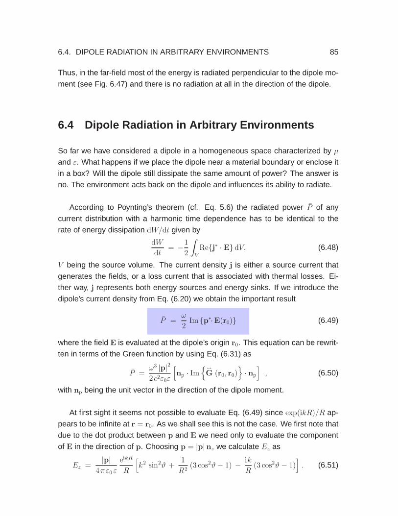
6.4. DIPOLE RADIATION IN ARBITRARY ENVIRONMENTS 85
Thus, in the far-field most of the energy is radiated perpendicular to the dipole mo-
ment (see Fig. 6.47) and there is no radiation at all in the direction of the dipole.
6.4 Dipole Radiation in Arbitrary Environments
So far we have considered a dipole in a homogeneous space characterized by µ
and ε. What happens if we place the dipole near a material boundary or enclose it
in a box? Will the dipole still dissipate the same amount of power? The answer is
no. The environment acts back on the dipole and influences its ability to radiate.
According to Poynting’s theorem (cf. Eq. 5.6) the radiated power P of any
current distribution with a harmonic time dependence has to be identical to the
rate of energy dissipation dW/dt given by
dW
dt= −1
2
∫
V
Rej∗ · E dV, (6.48)
V being the source volume. The current density j is either a source current that
generates the fields, or a loss current that is associated with thermal losses. Ei-
ther way, j represents both energy sources and energy sinks. If we introduce the
dipole’s current density from Eq. (6.20) we obtain the important result
P =ω
2Im p∗·E(r0) (6.49)
where the field E is evaluated at the dipole’s origin r0. This equation can be rewrit-
ten in terms of the Green function by using Eq. (6.31) as
P =ω3 |p|22c2ε0ε
[
np · Im
↔
G (r0, r0)
· np
]
, (6.50)
with np being the unit vector in the direction of the dipole moment.
At first sight it seems not possible to evaluate Eq. (6.49) since exp(ikR)/R ap-
pears to be infinite at r = r0. As we shall see this is not the case. We first note that
due to the dot product between p and E we need only to evaluate the component
of E in the direction of p. Choosing p = |p|nz we calculate Ez as
Ez =|p|
4πε0 ε
eikR
R
[
k2 sin2ϑ +1
R2(3 cos2ϑ− 1) − ik
R(3 cos2ϑ− 1)
]
. (6.51)

86 CHAPTER 6. RADIATION
Since the interesting part is the field at the origin of the dipole, the exponential term
is expanded into a series [exp(ikR) = 1 + ikR+ (1/2)(ikR)2 + (1/6)(ikR)3 + · · · ]and the limiting case R → 0 is considered. Thus,
dW
dt= lim
R→0
ω
2|p| ImEz=
ω |p|28πε0 ε
limR→0
2
3k3+R2 (..) + ..
=|p|212π
ω
ε0 εk3,
(6.52)
which is identical with Eq. (6.46). Thus, Eq. (6.49) leads to the correct result de-
spite the apparent singularity at R = 0.
The importance of Eq. (6.49) becomes obvious if we consider a dipole in an
inhomogeneous environment, such as an antenna next to the earth surface. The
rate at which energy is released can still be calculated by integrating the Poynt-
ing vector over a surface enclosing the dipole. However, to do this, we need to
know the electromagnetic field everywhere on the enclosing surface. Because of
the inhomogeneous environment, this field is not equal to the dipole field alone!
Instead, it is the self-consistent field, that is, the field E generated by the superpo-
sition of the dipole field and the scattered field from the environment (see Fig. 6.6).
Thus, to determine the energy dissipated by the dipole we first need to determine
the electromagnetic field everywhere on the enclosing surface. However, by using
Eq. (6.49) we can do the same job by only evaluating the total field at the dipole’s
origin r0.
As illustrated in Fig. 6.6, we decompose the electric field at the dipole’s position
Es
E0
p
Figure 6.6: Illustration of dipole radiation in inhomogeneous environments. The
total field is composed of a primary field E0 directly radiated by the dipole and
a secondary field Es that is emitted by the dipole and then scattered at inhomo-
geneities in the environment.

6.5. FIELDS EMITTED BY ARBITRARY SOURCES 87
as
E(r0) = E0(r0) + Es(r0) , (6.53)
where E0 and Es are the primary dipole field and the scattered field, respectively.
Introducing Eq. (6.53) into Eq. (6.49) allows us to split the rate of energy dissipa-
tion P = dW/dt into two parts. The contribution of E0 has been determined in
Eqs. (6.46) and (6.52) as
P0 =|p|212π
ω
ε0εk3 , (6.54)
which allows us to write for the normalized rate of energy radiation
P
P0
= 1 +6πε0 ε
|p|21
k3Imp∗ · Es(r0) (6.55)
Thus, the change of energy dissipation depends on the secondary field of the
dipole. This field corresponds to the dipole’s own field emitted at a former time. It
arrives at the position of the dipole after it has been scattered in the environment.
6.5 Fields Emitted by Arbitrary Sources
In Section 6.3.1 we have derived the vector potential A of a time-harmonic dipole
p. Using the scalar free-space Green function G0 we have then found a solution
for the vector potential of an arbitrary current distribution (see Eq. 6.30). The same
procedure can be applied to the electric field vector E.
According to Eq. (6.31) the E-field can be expressed in terms of a dyadic (ten-
sorial) Green function as E(r) = ω2µ0
↔
G0 (r, r′)p, where r′ is the origin of the
dipole. We can rewrite this equation as
E(r) = ω2µ0
∫
V
↔
G0 (r, r′′)p δ(r′ − r′′) dV ′′ (6.56)
Using Eq. (6.20) for the current density of a dipole [ j(r′′) = −iωpδ(r′−r′′)] and
substituting into Eq. (6.56) above, yields
E(r) = i ωµ0
∫
V
↔
G0 (r, r′) j(r′) dV ′ (6.57)

88 CHAPTER 6. RADIATION
rr'
E(r)j(r')G(r,r')
V
Figure 6.7: Illustration of the dyadic Green function↔
G (r, r′). The Green function
renders the electric field at the field point r due to a single point source j at the
source point r′. Since the field at r depends on the orientation of j the Green
function must account for all possible orientations in the form of a tensor.
where j now is an arbitrary current density distribution within the source volume V .
We could have derived Eq. (6.57) also by following a more formal way using the
definition of the Green function as described in Section 6.1. Fig. 6.7 illustrates the
meaning of Eq. (6.57): The volume V is subdivided into infinitesimal units, each
of which occupied by a point source with weight j(r′). In a similar way we find the
solution for the magnetic field as
H(r) =
∫
V
[∇×↔
G0 (r, r′)] j(r′) dV ′ (6.58)
Note that mathematically, the fields E and H above are particular solutions of the
differential equations (2.1) and (2.2). For a complete solution we need to super-
impose the homogeneous solutions, which are solutions of (2.1) and (2.2) with the
right sides being zero. These homogeneous solutions are fields that are present
even in absence of the sources j.
6.6 Sources with Arbitrary Time-Dependence
So far we have considered the fields generated by a source that is oscillating har-
monically in time with angular frequency ω. But what if the time dependence is

6.6. SOURCES WITH ARBITRARY TIME-DEPENDENCE 89
arbitrary, for example, a short pulse? In these cases we can employ Fourier trans-
forms, which describe an arbitrary time dependence by a superposition of time
harmonic dependences (see Section 2.2).
Let us go back to the time-harmonic solution (6.30) of the vector potential A.
We have pointed out in Section 2.2 that Maxwell’s equations for the Fourier trans-
forms of he fields (E, H, .. ) are formally the same as Maxwell’s equations for the
complex amplitudes (E(r), H(r), .. ). Therefore, Eq, (6.30) implies that
A(r, ω) = µ0
∫
V
G0(r, r′, ω) jtot(r
′, ω) dV ′ (6.59)
where, according to Eq. (6.26), G0 = exp(i k(ω) |r − r′|) / (4π|r−r′|), with k(ω) =
n(ω)ω/c. jtot denotes the Fourier transform of an arbitrary time-dependent current
density j(r, t), that is,
jtot(r, ω) =1
2π
∫ ∞
−∞
jtot(r, t) eiωt dt . (6.60)
The time-dependent vector potential A(r, t) of this current density is found by
Fourier transforming Eq. (6.59), which yields
A(r, t) =µ0
2π
∫
V
G0(r, r′, t) ∗ jtot(r
′, t) dV ′ , (6.61)
where ∗ denotes convolution in time and G0(r, r′, t) is given by
G0(r, r′, t) =
∫ ∞
−∞
G0(r, r′ω) e−iωt dω . (6.62)
Inserting the expression for G0 yields
G0(r, r′, t) =
∫ ∞
−∞
ei k(ω) |r−r′|
4π|r−r′| e−iωt dω =1
4π|r−r′|
∫ ∞
−∞
e−iω[t−n(ω)|r−r′|/c] dω .
(6.63)
In order to solve this integral we need to know the dependence of the index of
refraction n on frequency ω, which is referred to as dispersion. We assume that
n(ω) = n and obtain2
G0(r, r′, t) =
1
2
δ[t− |r− r′|n/c]|r−r′| . (6.64)
2∫
exp[ixy]dy = 2πδ[x].

90 CHAPTER 6. RADIATION
Thus, the Green function in time domain is a simple delta function evaluated at the
earlier time t′ = t−nR/c, where t is the current time and R is the distance between
source point r′ and observation point r.
We now insert G0(r, r′, t) into Eq. (6.61) and obtain
A(r, t) =µ0
4π
∫
V
∫
t′
δ[t′ − |r − r′|n/c]|r−r′| jtot(r
′, t− t′) dt′ dV ′
=µ0
4π
∫
V
jtot(r′, t− |r − r′|n/c)
|r−r′| dV ′ . (6.65)
A similar equation can be derived for the scalar potential φ(r). Taken both together
we have
A(r, t) =µ0
4π
∫
V
jtot(r′, t− |r − r′|n/c)
|r−r′| dV ′
φ(r, t) =1
4πε0
∫
V
ρtot(r′, t− |r− r′|n/c)
|r−r′| dV ′
(6.66)
(6.67)
These equations state that the fields A and φ at the location r and time t are deter-
mined by the sources jtot and ρtot at location r′ at the earlier time t−|r−r′|n/c. The
earlier time is a consequence of the speed of light c: it takes a time of |r−r′|n/c for
the fields to travel a distance of |r−r′| in a medium with index of refraction n. Thus,
Maxwell’s equations explain the mysterious “action-at-distance” phenomenon dis-
cussed in the introduction of this course (see Fig. 1). It has to be emphasized that
the index of refraction n is assumed to be dispersion-free, which is an approxima-
tion. The only material that is truly dispersion-free is vacuum (n = 1).
To find the fields E and H we insert the solutions of A and φ into Eqs. (6.7)
and (6.8). The calculation is not straightforward because A and φ depend on the
retarded time t − |r − r′|n/c. Therefore, an operation on the spatial coordinates
(e.g. ∇×) is implicitly also an operation on time. We will not go through this exer-
cise and only mention that the solution is identical with Eq. (2) if we express ρ and
j with the charge and current densities of a discrete charge (c.f. Eq. 3 and 4). The
result has three terms: the first term depends on the charge, the second term on
the velocity of the charge, and the third term on the acceleration of charge. It is
the latter that is associated with electromagnetic radiation.

6.6. SOURCES WITH ARBITRARY TIME-DEPENDENCE 91
The expression of fields in terms of retarded time is of limited practical value.
They help us to understand the physical origin of radiation but carrying out the in-
tegrals in Eqs. (6.66) and (6.67) is nearly impossible for realistic sources. Further-
more, the time-domain approach taken here is not able to accommodate dispersive
materials. Therefore, it is generally more favorable to process the fields in Fourier
space, that is, first calculate the spectrum of the source via Fourier transforma-
tion, then calculate the spectra of the fields, and finally taking the inverse Fourier
transform to express the fields in time domain. This procedure is shown in Fig. 6.8.
6.6.1 Dipole Fields in Time Domain
We have calculated the fields of a dipole with harmonic time dependence in Sec-
tion 6.3.2. These fields were expressed in spherical vector components (see
Eq. 6.41 - 6.43). Note that these fields are the complex amplitudes and that the
time-dependent fields are arrived at by multiplying with exp[−iωt] and taking the
real part.
Remember, that Maxwell’s equations for the complex amplitudes of time har-
monic fields (Eq. 2.31 - 2.34) are identical with Maxwell’s equations for the Fourier
transforms of fields with arbitrary time dependence (Eq. 2.25 - 2.28) . Therefore,
the solutions are identical as well. For example, the spectrum of the dipole’s Eϑ
field is
Eϑ(r, ω) = p(ω)sinϑ
4πε0ε(ω)
exp[ik(ω) r]
rk2(ω)
[
1
k2(ω) r2− i
k(ω) r− 1
]
, (6.68)
j(r,t)
j(r,ω) n(r,ω)
E(r,t)
E(r,ω)^^
Fourier Fourier
Maxwell
Figure 6.8: Calculating the field E of a time-dependent source j. Because of
dispersion and retardation it is favorable to solve for the fields in frequency space.

92 CHAPTER 6. RADIATION
in analogy to the corresponding complex amplitude in Eq. (6.42). We used p(ω) =
|p(ω)|. Note that dispersion is fully accounted for through ε(ω) and k(ω). Using
the time-dependent field Eϑ(r, t) can simply be calculated using the Fourier trans-
form (2.23).
To illustrate the transformation from frequency to time domain, we assume that
the dipole is in vacuum (k = ω/c and ε = 1). Also, we will only consider the far-field
term in Eq. (6.68). The time-dependent far-field Efϑ is calculated as
Efϑ(r, t) =
∫ ∞
∞
Efϑ(r, ω) e−iωt dω = −sin ϑ
4πε0
1
c2 r
∫ ∞
∞
ω2 p(ω) e−iω(t−r/c) dω . (6.69)
To solve this integral we set ω2 p(ω) = ψ(ω), where the Fourier transform of ψ(ω) is
ψ(t). Using the translation property of Fourier-transforms we obtain∫ ∞
∞
ψ(ω) e−iω(t−r/c) dω = ψ(t− r/c) . (6.70)
Thus, it remains to solve for ψ(t):
ψ(t) =
∫ ∞
∞
ω2 p(ω) e−iωt dω = − d2
dt2p(t) . (6.71)
Putting the pieces together we finally find
Efϑ(r, t) =
sin ϑ
4πε0
1
c2 r
d2 p(τ)
dτ 2
∣
∣
∣
∣
τ=t−r/c
(6.72)
Thus, the field at r = [r, ϑ, ϕ] and time t is determined by the dipole at r′ = 0 at
the earlier time t − r/c. As before, we find that it takes a time r/c for the “action”
to travel from the dipole to the observation point. Other terms of the dipole fields
(Eqs. 6.41 - 6.43) can be calculated following the same procedure. The result is
Er(t) =cosϑ
4πε0
[
2
r3+
2
c r2
d
dτ
]
p(τ)∣
∣
∣
τ=t−r/c
Eϑ(t) = −sin ϑ
4πε0
[
1
r3+
1
c r2
d
dτ+
1
c2r
d2
dτ 2
]
p(τ)∣
∣
∣
τ=t−r/c
Hϕ(t) = −sin ϑ
4πε0
√
ε0
µ0
[
1
c r2
d
dτ+
1
c2r
d2
dτ 2
]
p(τ)∣
∣
∣
τ=t−r/c
(6.73)
(6.74)
(6.75)
We see that the far-field is generated by the acceleration of the charges that con-
stitute the dipole moment. Similarly, the intermediate-field and the near-field are
generated by the speed and the position of the charges, respectively.

6.7. THE LORENTZIAN POWER SPECTRUM 93
6.7 The Lorentzian Power Spectrum
The spectrum of various physical processes is characterized by narrow lines de-
scribed by Lorentzian line shape functions. Examples are the spontaneous emis-
sion by atoms or molecules, laser radiation, or microwave resonators. To under-
stand the origin of Lorentzian line shapes we consider a dipole located at r0 = 0
that starts to oscillate at time t = 0. The observer is assumed to be at large dis-
tance from the dipole, which allows us to restrict the discussion to the dipole’s
far-field Efϑ(r, t).
The equation of motion for an undriven harmonically oscillating dipole is
d2
dt2p(t) + γ0
d
dtp(t) + ω2
0 p(t) = 0 . (6.76)
The natural frequency of the oscillator is ω0 and its damping constant is γ0. The
solution for p is
p(t) = Re
p0 e−iω0
√1−(γ2
0 /4ω20 ) t eγ0 t/2
. (6.77)
Typically, the damping constant is much smaller than the oscillation frequency
(γ0 ≪ ω0), which implies√
1 − (γ20/4ω
20) ≈ 1.
The spectrum Eϑ(ω) detected by the observer is (cf. Eq. (2.24))
Eϑ(ω) =1
2π
∫ ∞
r/c
Eϑ(t) eiωt dt. (6.78)
Here we set the lower integration limit to t = r/c because the dipole starts emitting
at t = 0 and it takes the time t = r/c for the radiation to propagate to the observa-
tion point. Therefore Eϑ(t< r/c) = 0. Inserting the solution for the dipole moment
from Eq. (6.77) and making use of γ0 ≪ ω0 we obtain after integration
Eϑ(ω) =1
2π
|p| sinϑω20
8πε0c2r
[
exp(iωr/c)
i(ω+ω0) − γ0/2+
exp(iωr/c)
i(ω−ω0) − γ0/2
]
. (6.79)
The energy radiated into the unit solid angle dΩ = sinϑdϑdϕ is calculated as
dW
dΩ=
∫ ∞
−∞
I(r, t)r2 dt = r2
√
ε0
µ0
∫ ∞
−∞
|Eϑ(t)|2 dt = 4πr2
√
ε0
µ0
∫ ∞
0
|Eϑ(ω)|2 dω ,
(6.80)

94 CHAPTER 6. RADIATION
where we applied Parseval’s theorem and used the definition of the intensity I =√
ε0/µ0 |Eϑ|2 of the emitted radiation. The total energy per unit solid angle dΩ and
per unit frequency interval dω can now be expressed as
dW
dΩ dω=
1
4πε0
|p|2 sin2ϑ ω20
4π2c3γ20
[
γ20/4
(ω−ω0)2 + γ20/4
]
(6.81)
The spectral shape of this function is determined by the expression in the brackets
known as the Lorentzian lineshape function. The function is shown in Fig. 6.9. The
width of the curve measured at half its maximum height is ∆ω = γ0, and is called
“radiative linewidth.”
Integrating the lineshape function over the entire spectral range yields a value
of πγ0/2. Integrating Eq. (6.81) over all frequencies and all directions leads to the
totally radiated energy
W =|p|24πε0
ω40
3 c3 γ0. (6.82)
This value is equal to the average power P radiated by a driven harmonic oscillator
divided by the linewidth γ0 (cf. Eq. 6.46).
ω0
ω
1
0.5 γ0
Figure 6.9: Lorentzian lineshape function as defined by the expression in brackets
in Eq. (6.81).

Chapter 7
Angular Spectrum Representation
The angular spectrum representation is a mathematical technique to describe op-
tical fields in homogeneous media. Optical fields are described as a superposition
of plane waves and evanescent waves which are physically intuitive solutions of
Maxwell’s equations. The angular spectrum representation is found to be a very
powerful method for the description of laser beam propagation and light focusing.
Furthermore, in the paraxial limit, the angular spectrum representation becomes
identical with the framework of Fourier optics which extends its importance even
further.
In this chapter we will consider purely monochromatic fields of angular fre-
quency ω, which can be represented as complex fields E(r) according to (c.f.
Chapter 2)
E(r, t) = ReE(r) e−iωt . (7.1)
In situations where the field is not time-harmonic, we we simply replace the com-
plex field E(r) by the spectrum E(r, ω) and obtain the time-dependent field by
Fourier transformation (see Section 2.2).
By the angular spectrum representation we understand the series expansion of
an arbitrary field in terms of plane (and evanescent) waves with variable amplitudes
and propagation directions (see Section 2.1.3). Assume we know the electric field
E(r) at any point r = (x, y, z) in space. For example, E(r) can be the solution of
an optical scattering problem, as shown in Fig. 7.1, for which E = Einc + Escatt. In
the angular spectrum picture, we draw an arbitrary axis z and consider the field E
95

96 CHAPTER 7. ANGULAR SPECTRUM REPRESENTATION
in a plane z=const. transverse to the chosen axis. In this plane we can evaluate
the two-dimensional Fourier transform of the complex field E(r) = E(x, y, z) as
E(kx, ky; z) =1
4π2
∞∫
−∞
∫
E(x, y, z) e−i [kxx+ kyy] dx dy , (7.2)
where x, y are the Cartesian transverse coordinates and kx, ky the corresponding
spatial frequencies or reciprocal coordinates. Similarly, the inverse Fourier trans-
form reads as
E(x, y, z) =
∞∫
−∞
∫
E(kx, ky; z) ei [kxx + ky y] dkx dky . (7.3)
Notice that in the notation of Eqs. (7.2) and (7.3) the field E = (Ex, Ey, Ez) and its
Fourier transform E = (Ex, Ey, Ez) represent vectors. Thus, the Fourier integrals
hold separately for each vector component.
So far we have made no requirements about the field E, but we will assume that
in the transverse plane the medium is homogeneous, isotropic, linear and source-
free. Then, a time-harmonic, optical field with angular frequency ω has to satisfy
Einc
Escatt
z
z = const.
Figure 7.1: In the angular spectrum representation the fields are evaluated in
planes (z = const.) perpendicular to an arbitrarily chosen axis z.

97
the vector Helmholtz equation (c.f. Eq. 2.12)
(∇2 + k2)E(r) = 0 , (7.4)
where k is determined by k = (ω/c)n and n =√µε is the index of refraction.
Inserting the Fourier representation of E(r) (Eq. 7.3) into the Helmholtz equation
and defining
kz ≡√
(k2 − k2x − k2
y ) with Imkz ≥ 0 , (7.5)
we find that the Fourier spectrum E evolves along the z-axis as
E(kx, ky; z) = E(kx, ky; 0) e±ikz z . (7.6)
The ± sign specifies that we have two solutions that need to be superimposed:
the + sign refers to a wave propagating into the half-space z > 0 whereas the −sign denotes a wave propagating into z < 0. Equation (7.6) tells us that the Fourier
spectrum of E in an arbitrary image plane located at z=const. can be calculated by
multiplying the spectrum in the object plane at z = 0 by the factor exp(±ikzz). This
factor is called the propagator in reciprocal space. In Eq. (7.5) we defined that
the square root leading to kz renders a result with positive imaginary part. This
ensures that the solutions remain finite for z→±∞. Inserting the result of Eq. (7.6)
into Eq. (7.3) we finally find for arbitrary z
E(x, y, z) =
∞∫
−∞
∫
E(kx, ky ; 0) ei [kxx+ kyy ± kzz] dkx dky (7.7)
which is known as the angular spectrum representation. In a similar way, we can
also represent the magnetic field H by an angular spectrum as
H(x, y, z) =
∞∫
−∞
∫
H(kx, ky ; 0) ei [kxx + ky y ± kz z] dkx dky . (7.8)
By using Maxwell’s equation H = (iωµµ0)−1 (∇×E) we find the following relation-
ship between the Fourier spectra E and H
Hx = Z−1µε [(ky/k) Ez − (kz/k) Ey] , (7.9)
Hy = Z−1µε [(kz/k) Ex − (kx/k) Ez] ,
Hz = Z−1µε [(kx/k) Ey − (ky/k) Ex] ,
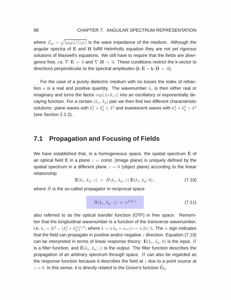
98 CHAPTER 7. ANGULAR SPECTRUM REPRESENTATION
where Zµε =√
(µ0µ)/(ε0ε) is the wave impedance of the medium. Although the
angular spectra of E and H fulfill Helmholtz equation they are not yet rigorous
solutions of Maxwell’s equations. We still have to require that the fields are diver-
gence free, i.e. ∇·E = 0 and ∇·H = 0. These conditions restrict the k-vector to
directions perpendicular to the spectral amplitudes (k·E = k·H = 0).
For the case of a purely dielectric medium with no losses the index of refrac-
tion n is a real and positive quantity. The wavenumber kz is then either real or
imaginary and turns the factor exp(±i kz z) into an oscillatory or exponentially de-
caying function. For a certain (kx, ky) pair we then find two different characteristic
solutions: plane waves with k2x + k2
y ≤ k2 and evanescent waves with k2x + k2
y > k2
(see Section 2.1.2).
7.1 Propagation and Focusing of Fields
We have established that, in a homogeneous space, the spatial spectrum E of
an optical field E in a plane z = const. (image plane) is uniquely defined by the
spatial spectrum in a different plane z = 0 (object plane) according to the linear
relationship
E(kx, ky; z) = H(kx, ky; z) E(kx, ky; 0) , (7.10)
where H is the so-called propagator in reciprocal space
H(kx, ky; z) = e±ikzz (7.11)
also referred to as the optical transfer function (OTF) in free space. Remem-
ber that the longitudinal wavenumber is a function of the transverse wavenumber,
i.e. kz = [k2 − (k2x + k2
y)]1/2, where k = n k0 = nω/c = n 2π/λ. The ± sign indicates
that the field can propagate in positive and/or negative z direction. Equation (7.10)
can be interpreted in terms of linear response theory: E(kx, ky; 0) is the input, H
is a filter function, and E(kx, ky; z) is the output. The filter function describes the
propagation of an arbitrary spectrum through space. H can also be regarded as
the response function because it describes the field at z due to a point source at
z = 0. In this sense, it is directly related to the Green’s function↔
G0.

7.1. PROPAGATION AND FOCUSING OF FIELDS 99
The filter H is an oscillating function for (k2x + k2
y) < k2 and an exponentially
decreasing function for (k2x + k2
y) > k2. Thus, if the image plane is sufficiently
separated from the object plane, the contribution of the decaying parts (evanescent
waves) is zero and the integration can be reduced to the circular area (k2x + k2
y) ≤k2. In other words, the image at z is a low pass filtered representation of the
original field at z = 0. The spatial frequencies (k2x + k2
y) > k2 of the original field
are filtered out during propagation and the information on high spatial variations
gets lost. Hence, there is always a loss of information on propagating from near-
to far-field and only structures with lateral dimensions larger than
∆x ≈ 1
k=
λ
2πn(7.12)
can be imaged with sufficient accuracy. Here, n is the index of refraction. This
equation is qualitative and we will provide a more detailed discussion later. In
general, higher resolution can be obtained by a higher index of refraction of the
embodying system (substrate, lenses, etc.) or by shorter wavelengths. Theoreti-
cally, resolutions down to a few nanometers can be achieved by using far-ultraviolet
radiation or X-rays.
Let us now determine how the fields themselves evolve. For this purpose we
denote the transverse coordinates in the object plane at z = 0 as (x′, y′) and in the
image plane at z = const. as (x, y). The fields in the image plane are described
by the angular spectrum (7.7). We just have to express the Fourier spectrum
E(kx, ky ; 0) in terms of the fields in the object plane. Similarly to Eq. (7.2) this
Fourier spectrum can be represented as
E(kx, ky; 0) =1
4π2
∞∫
−∞
∫
E(x′, y′, 0) e−i [kxx′ + kyy′] dx′ dy′ . (7.13)
After inserting into Eq. (7.7) we find the following expression for the field E in the
image plane z = const.
E(x, y, z) =1
4π2
∞∫
−∞
∫
E(x′, y′; 0)
∞∫
−∞
∫
ei [kx(x−x′)+ ky (y−y′)± kz z] dx′ dy′dkx dky
= E(x, y; 0) ∗ H(x, y; z) . (7.14)
This equation describes an invariant filter with the following impulse response

100 CHAPTER 7. ANGULAR SPECTRUM REPRESENTATION
(propagator in direct space)
H(x, y; z) =
∞∫
−∞
∫
ei [kxx + ky y ± kz z] dkx dky . (7.15)
H is simply the inverse Fourier transform of the propagator in reciprocal space H
(7.11). The field at z = const. is represented by the convolution of H with the field
at z=0.
7.1.1 Paraxial Approximation
In many optical problems the light fields propagate along a certain direction z and
spread out only slowly in the transverse direction. Examples are laser beam prop-
agation or optical waveguide applications. In these examples the wavevectors
k = (kx, ky, kz) in the angular spectrum representation are almost parallel to the
z-axis and the transverse wavenumbers (kx, ky) are small compared to k. We can
then expand the square root of Eq. (7.5) in a series as
kz = k√
1 − (k2x + k2
y)/k2 ≈ k −
(k2x + k2
y)
2 k. (7.16)
This approximation is called the paraxial approximation and it considerably simpli-
fies the analytical integration of the Fourier integrals. In the following we shall apply
the paraxial approximation to find a description for weakly focused laser beams.
7.1.2 Gaussian Beams
We consider a fundamental laser beam with a linearly polarized, Gaussian field
distribution in the beam waist
E(x′, y′, 0) = Eo e−x′2+y′2
w20 , (7.17)
where E0 is a constant field vector in the transverse (x, y) plane. We have chosen
z = 0 at the beam waist. The parameter w0 denotes the beam waist radius. We

7.1. PROPAGATION AND FOCUSING OF FIELDS 101
can calculate the spatial Fourier spectrum at z = 0 as1
E(kx, ky; 0) =1
4π2
∞∫
−∞
∫
E0 e−x′2+y′2
w20 e−i [kxx′ + kyy′] dx′ dy′
= E0w2
0
4πe−(k2
x+k2y)
w204 , (7.18)
which is again a Gaussian function. We now insert this spectrum into the an-
gular spectrum representation Eq. (7.7) and replace kz by its paraxial expression
in Eq. (7.16)
E(x, y, z) = E0w2
0
4 πeikz
∞∫
−∞
∫
e−(k2x+k2
y)(w2
04
+ iz2 k
) ei [kxx + ky y] dkx dky , (7.19)
This equation can be integrated and gives as a result the familiar paraxial repre-
sentation of a Gaussian beam
E(x, y, z) =E0 eikz
(1 + 2 iz/kw20)
e−
(x2+y2)
w20
1
(1 + 2 iz/kw20) . (7.20)
To get a better feeling for a paraxial Gaussian beam we set ρ2 = x2+y2, define a
new parameter z0 as
z0 =k w2
0
2, (7.21)
and rewrite Eq. (7.20) as
E(ρ, z) = E0w0
w(z)e− ρ2
w2(z) ei [kz−η(z)+kρ2/2R(z)] (7.22)
with the following abbreviations
w(z) = w0(1 + z2/z20)
1/2 beam radius (7.23)
R(z) = z(1 + z20/z
2) wavefront radius
η(z) = arctan z/z0 phase correction
The transverse size of the beam is usually defined by the value of ρ =√
x2 + y2
for which the electric field amplitude has decreased to a value of 1/e of its center
value
|E(x, y, z)| / |E(0, 0, z)| = 1/e . (7.24)

102 CHAPTER 7. ANGULAR SPECTRUM REPRESENTATION
It can be shown that the surface defined by this equation is a hyperboloid whose
asymptotes enclose an angle
θ =2
kw0(7.25)
with the z-axis. From this equation we can directly find the correspondence be-
tween the numerical aperture (NA = n sin θ) and the beam angle as NA ≈ 2n/kw0.
Here we used the fact that in the paraxial approximation, θ is restricted to small
beam angles. Another property of the paraxial Gaussian beam is that close to
the focus, the beam stays roughly collimated over a distance 2z0. z0 is called the
Rayleigh range and denotes the distance from the beam waist to where the beam
radius has increased by a factor of√
2. It is important to notice that along the z-axis
(ρ = 0) the phases of the beam deviate from those of a plane wave. If at z→−∞the beam was in phase with a reference plane wave, then at z→+∞ the beam will
be exactly out of phase with the reference wave. This phase shift is called Gouy
phase shift. The 180 phase change happens gradually as the beam propagates
through its focus. The phase variation is described by the factor η(z) in Eq. (7.23).
The tighter the focus the faster the phase variation will be.
A qualitative picture of a paraxial Gaussian beam and some of its characteris-
tics are shown in Fig. 7.2. It has to be emphasized that once the paraxial approx-
1∫
∞
−∞exp(−ax2 + ibx) dx =
√
π/a exp(−b2/4a) and∫
∞
−∞x exp(−ax2 + ibx) dx =
ib√
π exp(−b2/4a)/ (2a3/2)
z
θ ≈ 2/ kw0
ρ
2z0
ρ
1/e
w(z)
|E|
Figure 7.2: Illustration and main characteristics of a paraxial Gaussian beam. The
beam has a Gaussian field distribution in the transverse plane. The surfaces of
constant field strength form a hyperboloid along the z-axis.

7.2. FAR-FIELD APPROXIMATION 103
imation is introduced, the field E fulfills no longer Maxwell’s equations. The error
becomes larger the smaller the beam waist radius w0 is. Another important aspect
of Gaussian beams is that they do not exist, no matter how rigorous the theory that
describes them! The reason is that a Gaussian beam profile demands a Gaussian
spectrum. However, the Gaussian spectrum is infinite and contains evanescent
components that are not available in a realistic situation. Thus, a Gaussian beam
must always be regarded as an approximation. The tighter the focus, the broader
the Gaussian spectrum and the more contradictory the Gaussian beam profile will
be. The angular spectrum representation can be used to derive a rigorous descrip-
tion of focussed fields (e.g. Novotny, Principles of Nano-Optics).
7.2 Far-field Approximation
In this section we will derive the important result that Fourier Optics and Geomet-
rical Optics naturally emerge from the angular spectrum representation.
Consider a particular (localized) field distribution in the plane z = 0. The angu-
lar spectrum representation tells us how this field propagates and how it is mapped
onto other planes z = z0. Here, we ask what the field will be in a very remote plane.
Vice versa, we can ask what field will result when we focus a particular far-field onto
an image plane. Let us start with the familiar angular spectrum representation of
an optical field
E(x, y, z) =
∞∫
−∞
∫
E(kx, ky ; 0) ei [kxx+ kyy ± kzz] dkx dky . (7.26)
We are interested in the asymptotic far-zone approximation of this field, i.e. in the
evaluation of the field in a point r = r∞ at infinite distance from the object plane.
The dimensionless unit vector s in the direction of r∞ is given by
s = (sx, sy, sz) =(x
r,y
r,z
r
)
, (7.27)
where r= (x2 + y2 + z2)1/2 is the distance of r∞ from the origin. To calculate the
far-field E∞ we require that r → ∞ and rewrite Eq. (7.26) as
E∞(sx, sy) = limkr→∞
∫ ∫
(k2x+k2
y)≤k2
E(kx, ky ; 0) eikr [ kxk
sx +kyk
sy ± kzk
sz ] dkx dky , (7.28)
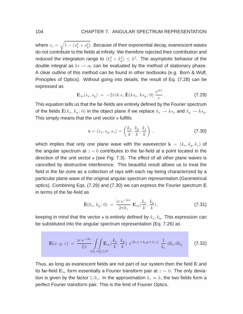
104 CHAPTER 7. ANGULAR SPECTRUM REPRESENTATION
where sz =√
1 − (s2x + s2
y). Because of their exponential decay, evanescent waves
do not contribute to the fields at infinity. We therefore rejected their contribution and
reduced the integration range to (k2x + k2
y) ≤ k2. The asymptotic behavior of the
double integral as kr→∞ can be evaluated by the method of stationary phase.
A clear outline of this method can be found in other textbooks (e.g. Born & Wolf,
Principles of Optics). Without going into details, the result of Eq. (7.28) can be
expressed as
E∞(sx, sy) = −2π ik sz E(ksx, ksy ; 0)eikr
r. (7.29)
This equation tells us that the far-fields are entirely defined by the Fourier spectrum
of the fields E(kx, ky ; 0) in the object plane if we replace kx → ksx and ky → ksy.
This simply means that the unit vector s fulfills
s = (sx, sy, sz) =
(
kx
k,ky
k,kz
k
)
, (7.30)
which implies that only one plane wave with the wavevector k = (kx, ky, kz) of
the angular spectrum at z = 0 contributes to the far-field at a point located in the
direction of the unit vector s (see Fig. 7.3). The effect of all other plane waves is
cancelled by destructive interference. This beautiful result allows us to treat the
field in the far-zone as a collection of rays with each ray being characterized by a
particular plane wave of the original angular spectrum representation (Geometrical
optics). Combining Eqs. (7.29) and (7.30) we can express the Fourier spectrum E
in terms of the far-field as
E(kx, ky ; 0) =ir e−ikr
2πkzE∞(
kx
k,ky
k) , (7.31)
keeping in mind that the vector s is entirely defined by kx, ky. This expression can
be substituted into the angular spectrum representation (Eq. 7.26) as
E(x, y, z) =ir e−ikr
2π
∫ ∫
(k2x+k2
y)≤k2
E∞(kx
k,ky
k) ei [kxx+ kyy ± kzz] 1
kz
dkx dky (7.32)
Thus, as long as evanescent fields are not part of our system then the field E and
its far-field E∞ form essentially a Fourier transform pair at z = 0. The only devia-
tion is given by the factor 1/kz. In the approximation kz ≈ k, the two fields form a
perfect Fourier transform pair. This is the limit of Fourier Optics.

7.2. FAR-FIELD APPROXIMATION 105
As an example consider the diffraction at a rectangular aperture with sides 2Lx
and 2Ly in an infinitely thin conducting screen which we choose to be our object
plane (z=0). A plane wave illuminates the aperture at normal incidence from the
back. For simplicity we assume that the field in the object plane has a constant
field amplitude E0 whereas the screen blocks all the field outside of the aperture.
The Fourier spectrum at z=0 is then
E(kx, ky; 0) =E0
4π2
∫ +Ly
−Ly
∫ +Lx
−Lx
e−i [kxx′ + kyy′] dx′ dy′
= E0LxLy
π2
sin(kx Lx)
kx Lx
sin(ky Ly)
ky Ly, (7.33)
With Eq. (7.29) we now determine the far-field as
E∞(sx, sy) = −ikszE02LxLy
π
sin(ksx Lx)
ksx Lx
sin(ksy Ly)
ksy Ly
eikr
r, (7.34)
s
z
z = 0
Figure 7.3: Illustration of the far-field approximation. According to the angular
spectrum representation, a point in the source plane z = 0 emits plane waves in all
possible directions. However, a distant detector (kr ≫ 1) measures only the plane
wave that propagates towards it (in direction of unit vector s). The fields of all other
plane waves are canceled by destructive interference.

106 CHAPTER 7. ANGULAR SPECTRUM REPRESENTATION
which, in the paraxial limit kz ≈k, agrees with Fraunhofer diffraction.
Equation (7.29) is an important result. It links the near-fields of an object with
the corresponding far-fields. While in the near-field a rigorous description of fields
is necessary, the far-fields are well approximated by the laws of Geometrical Op-
tics.
7.3 Fresnel and Fraunhofer Diffraction
Diffraction refers to the observation that light rays break away from their geometri-
cal paths, which is to say, that the wave nature of radiation becomes relevant. In
this section we will discuss two important regimes of diffraction theory, Fresnel and
Fraunhofer diffraction.
The far-field approximation derived in the previous chapter has its limitations. It
has been assumed that the observation point is at infinite distance from the source
plane. However, how far do we have to go to be approximately at infinity? The best
z = 0 z = const.
zx’
y’
x
yR
r
Figure 7.4: Coordinates used in discussion of Fresnel and Fraunhofer diffraction.

7.3. FRESNEL AND FRAUNHOFER DIFFRACTION 107
is to look at this question geometrically and to consider the situation illustrated in
Fig. 7.4. R is the observation distance defined as the distance from the origin in the
source plane (e.g. center of an aperture) to the observer. On the other hand, r is
the true distance between source point (x′, y′, 0) and the observation point (x, y, z).
The square of r calculated as
r2 = (x− x′)2 + (y − y′)2 + z2 = R2
[
1 − 2(xx′ + yy′)
R2+x′2+ y′2
R2
]
. (7.35)
After taking the square root on both sides and invoking the paraxial approximation
we obtain
r(x′, y′) = = R − [x′(x/R) + y′(y/R)] +x′2+ y′2
2R+ .. . (7.36)
To determine the field at the observation point, we have to sum up the waves
emanating from different locations in the source plane (x′, y′). This yields integrals
of the form∫
z=0
A(x′, y′)exp[−ikr(x′, y′)]
r(x′, y′)dx′ dy′ , (7.37)
where A(x′, y′) is some amplitude function. The ”summing up” of elementary
spherical waves is referred to as Huygens’ principle. Because of the large distance
between source and observer we can safely replace r(x′, y′) in the denominator by
R or z. However, we cannot apply this approximation to the exponent since we
would eliminate the effects of interference. Thus, we need to retain at least one of
the additional terms in the expansion of r in (7.36).
Let us denote the maximum extent of the sources at z = 0 as D, that is
D/2 = Max√
x′2 + y′2. If the observation distance is sufficiently large (R ≫ D),
we can neglect the last term in Eq. (7.36) and we end up with Fraunhofer diffrac-
tion. On the other hand, if the last term is not negligible, we speak of Fresnel
diffraction. Fresnel diffraction becomes considerably more complicated because
the exponent depends on the square of the source plane coordinates.
The transition from Fresnel to Fraunhofer diffraction happens at a distance
z that roughly corresponds to the Rayleigh range z0 of a Gaussian beam (c.f.
Eq. 7.21), that is, the distance where the beam transitions into a spherical wave.
Expressing the beam waist as w0 = D/2 we obtain
z0 =1
8k D2 . (7.38)

108 CHAPTER 7. ANGULAR SPECTRUM REPRESENTATION
As an example, let us consider a laser beam with beam diameter of D = 3 mm
and wavelength λ = 532 nm (green). It turns out that z0 = 13 m, which is quite a
distance to reach the far field!
7.4 The Point-Spread Function
The point-spread function is a measure of the resolving power of an imaging sys-
tem. The narrower the point-spread function the better the resolution will be. As
the name implies, the point-spread function defines the spread of a point source. If
object plane image plane
x
n1
n2
k1
k2
zf
2f
1
p
p
n1
n2
θ1 θ
2
f1
sin θ
1 = f
2 sin
θ
2
Figure 7.5: Calculation of the point-spread-function (PSF). The fields of a point
source are projected onto an image plane. Because of the loss of evanescent
waves and the finite angular collection angle of the imaging system, the point ap-
pears as a function with finite width.

7.4. THE POINT-SPREAD FUNCTION 109
we have a radiating point source then the image of that source will appear to have
a finite size. This broadening is a direct consequence of spatial filtering. A point in
space is characterized by a delta function that has an infinite spectrum of spatial
frequencies kx, ky. On propagation from the source to the image, high-frequency
components are filtered out. Usually the entire spectrum (k2x+k2
y)>k2 associated
with the evanescent waves is lost. Furthermore, not all plane wave components
can be collected, which leads to a further reduction in bandwidth. The reduced
spectrum is not able to accurately reconstruct the original point source and the
image of the point will have a finite size.
The smallest radiating electromagnetic unit is a dipole. As shown in Fig. 7.5, to
calculate the point-spread function (PSF) we have to trace the dipole’s field through
an imaging system that focuses it onto an image plane. We will choose the origin
of coordinates (x, y, z) = (0, 0, 0) at the focus and use the angular spectrum repre-
sentation of Eq. (7.32) to calculate the fields in the image plane. It is convenient to
represent Eq. (7.32) in spherical coordinates by using the substitutions
kx = k2 sin θ2 cosφ, ky = k2 sin θ2 sin φ, kz = k2 cos θ2 . (7.39)
Furthermore, due to the symmetry of our problem it is favorable to express the
transverse coordinates (x, y) of the field point as
x = ρ cosϕ y = ρ sinϕ . (7.40)
Finally, we note that the integration in Eq. (7.32) runs over a plane, which is not a
constant-coordinate surface in spherical coordinates. We therefore transform the
planar integration surface into a spherical one using
1
kzdkx dky = k2 sin θ2 dθ2 dφ , (7.41)
which is illustrated in Fig. 7.6.
Taken all together, the focal field represented by Eq. (7.32) can be written as
E(ρ, ϕ, z) =ik2f2 e−ik2f2
2π
Max[θ2]∫
0
2π∫
0
E∞(θ2, φ) eik2z cos θ2 eik2ρ sin θ2 cos(φ−ϕ) sin θ2 dφ dθ2
(7.42)

110 CHAPTER 7. ANGULAR SPECTRUM REPRESENTATION
Here, we have replaced the distance r∞ between the focal point and the surface
of the reference sphere of the lens by the focal length f2. We have also limited
the integration over θ2 to the finite range [0 ..Max[θ2]] because any lens will have
a finite size. Furthermore, since all fields propagate in the positive z-direction we
retained only the + sign in the exponent of Eq. (7.32).
To evaluate Eq. (7.42) we need to insert the field E∞ of the dipole after it has
been refracted by the lens. To simplify the analysis we will ignore the vectorial
nature of dipole and its fields. Furthermore, we will assume that the imaging sys-
tem can be treated in the paraxial approximation, or small angle limit, for which
sin θ1 ≈ θ1 and sin θ2 ≈ θ2. Using the far-field term of Eq. (6.42) and ignoring the
angular dependence (scalar point source), the dipole field before refraction at the
lens is
E1 = − p k21
4πε0ε1
exp(ik1f1)
f1. (7.43)
We trace this field through the lens and then insert it as E∞ into Eq. (7.42) above.
In essence, the dipole field is a field that uniformly illuminates the focusing lens,
that is E∞(θ2, φ) ≈ const.. Using the mathematical relation
2π∫
0
eix cos(φ−ϕ) dφ = 2π J0(x) , (7.44)
we can carry out the integration over φ analytically. Here, J0 is the 0th-order Bessel
k22 sinθ
2 dθ
2 dφ
kz
θ2
dkx dky
dkx dky = cosθ2 [k
22 sinθ
2 dθ
2 dφ]
Figure 7.6: Illustration of the substitution (1/kz) dkx dky = k sin θ dθ dφ. The factor
1/kz = 1/(k cos θ) ensures that the differential areas on the plane and the sphere
stay equal.

7.4. THE POINT-SPREAD FUNCTION 111
function. The final expression for the focal field now contains a single integration
over the variable θ2. Skipping the constant prefactors we obtain
E(ρ, ϕ, z) ∝Max[θ2]∫
0
eik2z cos θ2 J0(k2ρ sin θ2) sin θ2 dφ dθ2 . (7.45)
Using sin θ2≈θ2, setting z = 0 (image plane), and using∫
xJ0(x)dx = xJ1(x) , (7.46)
we find the following result for the intensity in the image plane
limθmax≪π/2
∣
∣E(ρ, z=0)∣
∣
2=
π4
ε20n1n2
p2
λ6
NA4
M2
[
2J1(2πρ)
(2πρ)
]2
, ρ =NA ρMλ
(7.47)
Here, we have used a normalized coordinate ρ, which is expressed in terms of the
magnification M = (n1/n2)(f2/f1) and the numerical aperture
NA = n1 sin(Max[θ1]) . (7.48)
Note that sin(Max[θ1]) = (f2/f1) sin(Max[θ2]). The result (7.47) is the point-spread-
function, first derived by Abbe in 1873. Its functional form is given by the term in
object plane image plane
M ΔxΔx
Figure 7.7: Illustration of the resolution limit. Two simultaneously radiating point
sources separated by ∆r|| in the object plane generate a combined point-spread
function in the image plane. The two point sources are resolved if they can be
distinguished based on their image pattern.

112 CHAPTER 7. ANGULAR SPECTRUM REPRESENTATION
brackets which is known as the Airy function. It tells us that the image of a point
is no longer a point, but a function with a finite width. This width determines the
resolution of an imaging system. In essence, two points in the object plane have
to be separated by more than the width of the PSF in order to be distinguishable.
This is illustrated in Fig. 7.7.
The point-spread function can be measured by using a single quantum emitter,
such as a single molecule of quantum dot, as a point emitter. Fig. 7.8 shows such a
measurement together with a fit according to Eq. (7.47). The point-spread-function
has been recorded by using a NA = 1.3 lens to collect the fluorescence photons
from a single DiI molecule with center wavelength of λ ≈ 580 nm.
The width of the point-spread function ∆x is usually defined as the radial dis-
30
25
20
15
10
5
0-1.0 -0.5 0 0.5 1.0
distance (μm)
ph
oto
n c
ou
nt ra
te (
kH
z)
Figure 7.8: Point-spread function measured with a single molecule point source.
Fluorescence photons emitted by a DiI molecule are collected with a NA = 1.3
objective lens. The center wavelength is λ ≈ 580 nm. The data points correspond
to a horizontal line cut through the center of the fluorescence rate image shown in
the inset. The solid curve corresponds to the Airy function.

7.4. THE POINT-SPREAD FUNCTION 113
tance for which the value of the paraxial point-spread function becomes zero, or
∆x = 0.6098M λ
NA. (7.49)
This width is also denoted as the Airy disk radius. It depends in a simple manner
on the numerical aperture, the wavelength and the magnification of the system.

114 CHAPTER 7. ANGULAR SPECTRUM REPRESENTATION

Chapter 8
Waveguides and Resonators
The objective of resonators is to confine electromagnetic energy. On the other
hand, the purpose of waveguides is to guide electromagnetic energy. In both
cases, the desired functionality is achieved through material boundaries.
8.1 Resonators
Let us consider a rectangular box with sides Lx, Ly, and Lz, as shown in Fig. 8.1.
The interior of the box is filled with a linear and isotropic material characterized
by ε and µ. The walls of the box are perfectly reflecting, that is, the fields are not
able to penetrate into the walls. Furthermore, there are no sources present, which
implies that we’re looking for homogeneous solutions of the wave equation, that is,
solutions of the Helmholtz equation (3.15).
To solve the Helmholtz equation for the x component of the complex electric
field vector E we write
Ex(x, y, z) = E(x)0 X(x) Y (y)Z(z) , (8.1)
which is referred to as separation of variables. X, Y , and Z are dimensionless
functions and E(x)0 is a constant field amplitude. Inserting into [∇2 + k2]Ex = 0
yields1
X
∂2X
∂x2+
1
Y
∂2Y
∂y2+
1
Z
∂2Z
∂z2+ k2 = 0 . (8.2)
115

116 CHAPTER 8. WAVEGUIDES AND RESONATORS
In order for this equation to hold for any x, y, and z we have to require that each
of the terms is constant. We set these constants to be −k2x, −k2
y and −k2z , which
implies
k2x + k2
y + k2z = k2 =
ω2
c2n2(ω) . (8.3)
We obtain three separate equations for X, Y , and Z
∂2X /∂x2 + k2xX = 0
∂2Y / ∂y2 + k2yY = 0
∂2Z / ∂z2 + k2zZ = 0 , (8.4)
with the solutions exp[±ikxx], exp[±ikyy], and exp[±ikzz]. Thus, the solutions for
Ex become
Ex(x, y, z) = E(x)0 [c1,x e−ikxx + c2,x eikxx] [c3,x e−ikyy + c4,x eikyy] [c5,x e−ikzz + c6,x eikzz] .
(8.5)
Electric fields cannot penetrate into a perfect conductor. Therefore, the boundary
condition (4.13) implies Ex(x = 0) = Ex(x = Lx) = 0, which turns Eq. (8.5) into
Ex(x, y, z) = E(x)0 sin[nπ x/Lx] [c3,x e−ikyy + c4,x eikyy] [c5,x e−ikzz + c6,x eikzz] , (8.6)
x
y
zLz
Lx
Ly
Figure 8.1: A resonator with perfectly reflecting walls and side lengths Lx, Ly, and
Lz .

8.1. RESONATORS 117
with n being an integer. Similar solutions are found for Ey and Ez, namely,
Ey(x, y, z) = E(y)0 [c1,y e−ikxx + c2,y eikxx] sin[mπ y/Ly] [c5,y e−ikzz + c6,y eikzz] (8.7)
Ez(x, y, z) = E(z)0 [c1,z e−ikxx + c2,z eikxx] [c3,z e−ikyy + c4,z eikyy] sin[l π z/Lz]. (8.8)
Because ∇ · E = 0 for any x, y, and z we find
Ex(x, y, z) = E(x)0 sin[nπ x/Lx] sin[mπ y/Ly] sin[l π z/Lz]
Ey(x, y, z) = E(y)0 sin[nπ x/Lx] sin[mπ y/Ly] sin[l π z/Lz ]
Ez(x, y, z) = E(z)0 sin[nπ x/Lx] sin[mπ y/Ly] sin[l π z/Lz] , (8.9)
andn
Lx
E(x)0 +
m
Ly
E(y)0 +
l
Lz
E(z)0 = 0 (8.10)
Using Eq. (8.3) we find the dispersion relation or mode structure of the resonator
π2
[
n2
L2x
+m2
L2y
+l2
L2z
]
=ω2
nml
c2n2(ωnml) n,m, l ∈ 0, 1, 2, 3, .. (8.11)
Thus, we find that the resonator supports only discrete frequencies ωnml, each as-
sociated with a mode (n,m, l) of the resonator. Note that n is used both for the
index of refraction and for the mode number in x.
8.1.1 The Density of States
Let us now consider a resonator with equal sides, that is, L = Lx +Ly +Lz. In this
case,
n2 +m2 + l2 =
[
ωnml Ln(ωnml)
π c
]2
. (8.12)
If n, m, and l were real numbers, then this equation defines a sphere of radius
r0 = [omeganml Ln(ωnml)/(π c)]. Indeed, for large numbers we can approximate
these numbers by real numbers. Let us now consider a specific mode given by
[n,m, l] and with angular frequency ω = ωnml and count the number of modes N
with frequencies smaller than ω. According to Eq. (8.12) this corresponds to the
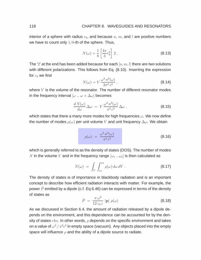
118 CHAPTER 8. WAVEGUIDES AND RESONATORS
interior of a sphere with radius r0, and because n, m, and l are positive numbers
we have to count only 1/8-th of the sphere. Thus,
N(ω) =1
8
[
4π
3r30
]
2 . (8.13)
The ‘2’ at the end has been added because for each [n,m, l] there are two solutions
with different polarizations. This follows from Eq. (8.10). Inserting the expression
for r0 we find
N(ω) = Vω3 n3(ω)
3π2 c3, (8.14)
where V is the volume of the resonator. The number of different resonator modes
in the frequency interval [ω .. ω + ∆ω] becomes
dN(ω)
dω∆ω = V
ω2 n3(ω)
π2 c3∆ω , (8.15)
which states that there a many more modes for high frequencies ω. We now define
the number of modes ρ(ω) per unit volume V and unit frequency ∆ω. We obtain
ρ(ω) =ω2 n3(ω)
π2 c3(8.16)
which is generally referred to as the density of states (DOS). The number of modes
N in the volume V and in the frequency range [ω1 .. ω2] is then calculated as
N(ω) =
∫
V
∫ ω2
ω1
ρ(ω) dω dV . (8.17)
The density of states is of importance in blackbody radiation and is an important
concept to describe how efficient radiation interacts with matter. For example, the
power P emitted by a dipole (c.f. Eq 6.46) can be expressed in terms of the density
of states as
P =π ω2
12 ε0 ε|p| ρ(ω) (8.18)
As we discussed in Section 6.4, the amount of radiation released by a dipole de-
pends on the environment, and this dependence can be accounted for by the den-
sity of states rho. In other words, ρ depends on the specific environment and takes
on a value of ω2 / π2c3 in empty space (vacuum). Any objects placed into the empty
space will influence ρ and the ability of a dipole source to radiate.

8.1. RESONATORS 119
The resonator that we have analyzed possesses discrete frequencies ωmnl. In
reality, any resonator has losses, for example due to the absorption of electromag-
netic energy at the boundaries or due to radiation. As a consequence, the discrete
frequencies broaden and assume a finite line width ∆ω = 2γ. The quality factor,
or Q-factor of a line is defined as Q = ω/(2γ). It is a measure for how long elec-
tromagnetic energy can be stored in a resonator. The line shape of a mode is
generally a Lorentzian (see Section 6.7). The electric field in the cavity is therefore
an exponentially damped oscillation of the form
E(r, t) = Re
E0(r) exp
[
(iω0 −ω0
2Q) t
]
, (8.19)
where ω0 represents one of the resonance frequencies ωmnl. The spectrum of the
stored energy density becomes
Wω(ω) =ω2
0
4Q2
Wω(ω0)
(ω − ω0)2 + (ω0 / 2Q)2. (8.20)
8.1.2 Cavity Perturbation
A sharp resonance is a key requirement for ultrasensitive detection in various ap-
plications. For example, watches and clocks use high-Q quartz crystals to mea-
sure time, some biosensing schemes make use of oscillating cantilevers to detect
adsorption of molecules, and atomic clocks use atomic resonances as frequency
standards. A perturbation of the resonator (cavity), for example due to particle
adsorption or a change of the index of refraction, leads to a shift of the resonance
frequency, which can be measured and used as a control signal for sensing.
To establish an understanding of cavity perturbation we consider the system
depicted in Fig. 8.2. A leaky cavity and its environment are characterized by a
spatially varying permittivity ε(r) and permeability µ(r). In the absence of any
perturbation the system assumes a resonance at frequency ω0 and the the fields
are described by
∇× E0 = iω0µ0µ(r)H0 , ∇×H0 = −iω0ε0ε(r)E0 , (8.21)
with E0(r, ω0) and H0(r, ω0) denoting the unperturbed complex field amplitudes. A
particle with material parameters ∆ε(r), ∆µ(r) constitutes a perturbation and gives

120 CHAPTER 8. WAVEGUIDES AND RESONATORS
rise to a new resonance frequency ω. Maxwell’s curl equations for the perturbed
system read as
∇× E = iωµ0 [µ(r)H + ∆µ(r)H] (8.22)
∇× H = −iωε0 [ε(r)E + ∆ε(r)E] . (8.23)
Notice that both ∆ε and ∆µ are zero outside of the volume occupied by the per-
turbation. Using ∇ · (A× B) = (∇× A) · B − (∇×B) · A we find
∇ · [E∗0 × H− H∗
0 × E] = i(ω − ω0) [ε0ε(r)E∗0 · E + µ0µ(r)H∗
0 · H]
+ iω [E∗0ε0∆ε(r)E + H∗
0µ0∆µ(r)H] . (8.24)
We now consider a fictitious spherical surface ∂V at very large distance from the
cavity and integrate Eq. (8.24) over the enclosed volume V (c.f. Fig. 8.2). Using
Gauss’ theorem, the left hand side of Eq. (8.24) becomes∫
∂V
[H · (n ×E∗0) + H∗
0 · (n ×E)] da = 0 (8.25)
where n is a unit vector normal to the surface ∂V . The above expression vanishes
because of the transversality of the field, i.e. (n×E∗0) = (n×E) = 0 on the surface
ΔV
resonator
perturbation
∂V
enclosing surface
Figure 8.2: A resonator with resonance frequency ω0 interacts with an external
perturbation giving rise to a new resonance frequency ω. The calculation makes
use of a fictitious spherical surface at infinity.

8.1. RESONATORS 121
of the spherical surface. We thus arrive at the equation
ω − ω0
ω= −
∫
V[E∗
0 ε0∆ε(r)E + H∗0µ0∆µ(r)H] dV
∫
V[ε0ε(r)E∗
0 · E + µ0µ(r)H∗0 · H] dV
, (8.26)
which is known as the Bethe-Schwinger cavity perturbation formula. Eq. (8.26) is
an exact formula, but because E and H are not known the equation cannot be
used in its form. Notice that because ∆ε and ∆µ are zero outside of the volume
occupied by the perturbation the integral in the nominator runs only over the vol-
ume of the perturbation ∆V . For situations where there are no radiation losses
and all the energy is contained inside the boundaries of a resonator the surface
∂V can be chosen to coincide with the boundaries.
We assume that the perturbation has a small effect on the cavity. Therefore we
write as a first-order approximation E = E0 and H = H0. After performing these
substitutions in Eq. (8.26) we find
ω − ω0
ω≈ −
∫
∆V[E∗
0 ε0∆ε(r)E0 + H∗0µ0∆µ(r)H0] dV
∫
V[ε0ε(r)E
∗0 · E0 + µ0µ(r)H∗
0 · H0] dV(8.27)
For a high-Q resonator the radiation losses are small and the integration volume
V can be taken over the boundaries of the resonator. To evaluate Eq. (8.27) we
first must solve for the fields E0(r),H0(r) of the unperturbed cavity. Interestingly,
for a weakly-dispersive medium the denominator of Eq. (8.27) denotes the total
energy of the unperturbed cavity (W0) whereas the nominator accounts for the
energy introduced by the perturbation (∆W ). Hence, (ω − ω0)/ω = −∆W/W0.
An increase of energy by ∆W causes the resonance frequency to red-shift to
ω = ω0 [W0/(W0 + ∆W )]. A blue-shift is possible by perturbing the cavity volume,
i.e. by removing ∆W from the cavity.
As an example let us consider a planar cavity with perfectly reflecting end faces
of area A and separated by a distance L. The fundamental mode λ = 2L has a
resonance frequency ω0 = πc/L, and the electric and magnetic fields inside the
cavity are calculated to be E0 sin[πz/L] and −i√
ε0/µ0E0 cos[πz/L], respectively.
The coordinate z is perpendicular to the surfaces of the end faces. The denomi-
nator of Eq. (8.27) is easily determined to be V ε0E20 , where V = LA. We place a
spherical nanoparticle with dielectric constant ∆ε and volume ∆V in the center of

122 CHAPTER 8. WAVEGUIDES AND RESONATORS
the cavity and assume that the field is homogeneous across the dimensions of the
particle. The nominator of Eq. (8.27) is calculated to be ∆V ∆ε ε0E20 and the fre-
quency shift is determined to be (ω − ω0)/ω = −∆ε∆V/V . A better approximation
retains the perturbed fields E and H in the nominator of Eq. (8.26). Making use of
the quasi-static solution for a small spherical particle we write E = 3E0/(2 + ∆ε)
and obtain a frequency shift of (ω − ω0)/ω = −[3∆ε/(2 + ∆ε)] ∆V/V . In both cases
the resonance shift scales with the ratio of resonator and perturbation volumes.
8.2 Waveguides
Waveguides are used to carry electromagnetic energy from location A to location
B. They exist in form of wires, coaxial cables, parallel plates, or optical fibers. In
general, the transmission of radiation through free-space is subject to diffraction,
which results in spreading out of energy. Waveguides avoid this problem at the
expense of material structures that have to connect the locations A and B.
The simplest waveguide system is the two-wire transmission line. It can be
formulated in terms of distributed circuit elements, such as capacitances C and
inductances L. One can derive a one-dimensional wave equation for the current
and the voltage carried along the transmission line. The speed of propagation is
given by c = 1/√LC. Detailed discussions of transmission lines can be found in
many textbooks and we won’t derive or analyze it here. Instead, we will concen-
trate on parallel-plate waveguide and on hollow metal waveguides and then make
a transition to all-dielectric waveguides used in fiber-optic communication.
8.2.1 Parallel-Plate Waveguides
The parallel-plate waveguide that we consider here is illustrated in Fig. 8.3. It
consists of a medium characterized by the index of refraction n(ω) sandwiched be-
tween two ideally conducting plates. We will align our coordinate system such that
the wave propagates in direction of the z axis. As we shall see, one distinguishes
between two different solutions: 1) Waves that have no electric field in propagation

8.2. WAVEGUIDES 123
direction z (TE modes), and 2) waves that have no magnetic field in propagation
direction z (TM modes).
TE Modes
For TE modes the electric field is parallel to the surface of the plates. As an ansatz
we choose a plane wave propagating at an angle θ towards the bottom plate
E1(x, y, z) = E0 ny exp[−ikx cos θ + ikz sin θ] , (8.28)
with k = n(ω)ω/c. The wave reflects at the bottom plate and then propagates
towards the top plate
E2(x, y, z) = −E0 ny exp[ikx cos θ + ikz sin θ] , (8.29)
where the sign change is due to the boundary condition, that is, the total parallel
E-field has to vanish. The sum of the fields becomes
E(x, y, z) = E1(x, y, z) + E2(x, y, z) = −2i E0 ny exp[ikz sin θ] sin[kx cos θ] .
(8.30)
While this field satisfies the boundary condition at the bottom surface, it does not
yet at the top plate x = d. Requiring that E(d, y, z) = 0 yields sin[kx cos θ] = 0,
which is fulfilled if
kd cos θ = nπ n ∈ 1, 2, .. , (8.31)
which corresponds to a ‘quantization’ of the normal wavenumber kx = k cos θ
kxn = nπ
dn ∈ 1, 2, .. . (8.32)
x
y
z
d
k
Figure 8.3: A parallel-plate waveguide with plate separation d.

124 CHAPTER 8. WAVEGUIDES AND RESONATORS
Note that n = 0 is excluded because it yields a zero-field (trivial solution). Using
k2 = k2z + k2
x, we find the the propagation constant kz of the field propagating in
between of the plates in z direction is
kzn =√
k2 − n2 [π/d]2 n ∈ 1, 2, .. (8.33)
As long as kzn is real the field will propagate along the z direction. However, when
nπ/d > k the propagation constant kzn is imaginary and the field will exponential
decay in direction of z, similar to evanescent waves discussed in Section 4.4. Be-
cause k ∝ ω it turns out that the waveguide acts as a high-pass filter. Frequencies
below the cut-off frequency
ωc =nπ c
d n(ωc)n ∈ 1, 2, .. (8.34)
cannot propagate. In summary, the solutions of the wave equation for a system of
two parallel plates are characterized by a mode number n. We refer to the solu-
tions that have no electric field in propagation direction as TEn modes. Solutions
are found only for discrete frequencies ωn and for each mode there is a cut-off fre-
quency below which no propagation is possible. Note, that n(ωc) is the dispersive
index of refraction of the medium between the two plates.
For propagating fields with ω > ωc, the phase velocity is defined by the phase
factor exp[ikznz − iωt] as vph = ω/kzn. On the other hand, the energy of the field
and thus any information associated with it is transported at the group velocity
vg = dω/dkzn.
TM Modes
Let us now repeat the analysis for the case where the magnetic field is parallel to
the surface of the plates. Similar to Eq. (8.28) we write
H1(x, y, z) = H0 ny exp[−ikx cos θ + ikz sin θ] , (8.35)
The wave reflects at the bottom plate and then propagates towards the top plate
H2(x, y, z) = H0 ny exp[ikx cos θ + ikz sin θ] , (8.36)

8.2. WAVEGUIDES 125
In contrast to Eq. (8.36) there is no sign change of H0 upon reflection at the bound-
ary. This follows from the boundary conditions (4.11) - (4.14).1 The sum of the
fields becomes
H(x, y, z) = H1(x, y, z)+H2(x, y, z) = 2H0 ny exp[ikz sin θ] cos[kx cos θ] , (8.37)
and the boundary conditions at the top interface z = d lead to the condition
kd cos θ = nπ n ∈ 0, 1, 2 .. . (8.38)
In contrast to the quantization condition (8.31) for TE modes, we now also find
solutions for n = 0 (cos(0) 6= 0). Thus,
kzn =√
k2 − n2 [π/d]2 n ∈ 0, 1, .. (8.39)
The fundamental mode TM0 has no cut-off frequency whereas all higher order TM
do have a cut-off, similar to TE modes discussed above. The absence of a cut-off1The electric field associated with H1 is E1 ∼ E0[sin θ, 0, cos θ]T , which upon reflection becomes
E2 ∼ E0[sin θ, 0,− cos θ]T because the parallel E-field at the boundary has to vanish. Consequently,H0 remains unchanged upon reflection.
0
0.2
0.4
1.0
0.6
0.8
0 0.5 1.0 1.5 2.0 2.5 3.0
TM0
TM1
TM2
TM3
TM4
TM5
TE1
TE2
TE3
TE4
TE5
kz / k
d / λ
Figure 8.4: Mode structure of a parallel-plate waveguide with plate separation d.
The vertical axis shows the real part of the normalized propagation constant. All
modes, with the exception of TM0 run into cut-off as the wavelength λ is increased
or the plate separation d is decreased.

126 CHAPTER 8. WAVEGUIDES AND RESONATORS
for the TM mode is a finding that is not restricted to two parallel plates, but holds
for any waveguide made of two electrically isolated metal electrodes. For example,
a coaxial cable has no cut-off, but a hollow metal waveguide (a pipe) does have a
cut-off.
8.2.2 Hollow Metal Waveguides
We now confine the lateral extent of the waveguide modes. The parallel-plate
waveguide then turns into a hollow metal waveguide as illustrated in Fig. 8.5. To
solve for the fields in such a waveguide structure we write
E(x, y, z) = Exy(x, y) e−ikzz . (8.40)
Inserting into the the Helmholtz equation (3.15) leads to
[
∇2t + k2
t
]
Exy(x, y) = 0 , (8.41)
where ∇2t = ∂2/∂x2+∂2/∂y2 is the transverse Laplacian and and kt = [k2
x+k2y]
1/2 =
[k2 − k2z ]
1/2 is the transverse wavenumber.
Next, we write the electric field in terms of a transverse vector in the (x,y) plane
and a longitudinal vector that points along the z axis, that is,
E = Et + Ez . (8.42)
z
x
y
Lx
Ly
Figure 8.5: A rectangular hollow metal waveguide.

8.2. WAVEGUIDES 127
Here, Et = E × nz and Ez = (E · nz)nz. A similar expression can be written for
the magnetic field H. Inserting both expressions into Maxwell’s equations (2.31)
- (2.34), and assuming that the waveguide materials is linear and source-free, we
find
Exyx = −Z ik
k2t
∂Hxyz
∂y+ikz
k2t
∂Exyz
∂x(8.43)
Exyy = Z
ik
k2t
∂Hxyz
∂x+ikz
k2t
∂Exyz
∂y(8.44)
Hxyx = Z−1 ik
k2t
∂Exyz
∂y+ikz
k2t
∂Hxyz
∂x(8.45)
Hxyy = −Z−1 ik
k2t
∂Exyz
∂x+ikz
k2t
∂Hxyz
∂y. (8.46)
where Z is the wave impedance defined in Eq. (4.33). These equations show that
the transverse field components Exyx , Exy
y and Hxyx , Hxy
y derive from the longitudinal
field components Exyz and Hxy
z . Thus, it is sufficient to solve for Exyz and Hxy
z . So
far, the discussion was general, not restricted to any particular waveguide geome-
try. We next discuss the particular case of a rectangular hollow metal waveguide,
as illustrated in Fig. 8.5. Such waveguides are commonly used in the microwave
regime, which spans the frequency range of 1-100 GHz.
TE Modes
For TE waves the field Exyz is zero. Thus, according to Eqs. (8.43) - (8.46) all field
components can be derived from Hxyz . Following the discussion in Section 8.2.1
we find
Hxyz (x, y) = H0z cos[kxx] cos[kyy] (8.47)
= H0z cos[nπ
Lx
x] cos[mπ
Ly
y] n,m ∈ 0, 1, 2 .. ,
with the transverse wavenumber given by
k2t = [k2
x + k2y ] =
[
n2π2
L2x
+m2π2
L2y
]
n,m ∈ 0, 1, 2 .. , (8.48)

128 CHAPTER 8. WAVEGUIDES AND RESONATORS
similar to the mode structure of a resonator (Eq. 8.11). Accordingly, the frequen-
cies of the TEnm modes are
ωnm =π c
n(ωnm)
√
n2
L2x
+m2
L2y
n,m ∈ 0, 1, 2, .. (8.49)
with n(ωnm) being the index of refraction. It turns out that n and m cannot both
be zero because the TE00 does not exist. Thus, the lowest frequency mode is the
TE01 or the TE10 mode. While the modes of a parallel-plate waveguide are formed
by the superposition of two plane waves, the fields of a hollow rectangular waveg-
uide follow from the superposition of four plane waves. Note that the condition
of a magnetic field parallel to the waveguide surfaces leads here to TE modes,
whereas in the case of two parallel plates it leads to TM modes.
The propagation constant (longitudinal wavenumber) is calculated as
kz =√
k2 − k2t =
√
ω2nm
c2n2(ωnm) −
[
n2π2
L2x
+m2π2
L2y
]
n,m ∈ 0, 1, 2 .. .
(8.50)
Since n, m cannot both be zero we find that all modes run into cut-off for low
enough frequencies ω. The lowest-order mode is generally referred to as the fun-
damental mode or the dominant mode.
Let us choose Lx > Ly. In this case, the fundamental mode is the TE01 mode
for which, according to Eqs. (8.43) - (8.46), the fields are determined as
Hxyz = H0z cos[
π
Ly
y] (8.51)
Hxyy = i(kz/k
2t )H0z (π/Ly) sin[
π
Lyy] (8.52)
Exyx = −(ikZ/k2
t )H0z (π/Ly) sin[π
Lyy] (8.53)
Hxyx = Exy
y = Exyz = 0 .
According to Eq. (8.40), the total fields E and H are obtained by multiplying with
exp[−ikzz]. The fields of the TE01 mode are illustrated in Fig. 8.6.

8.2. WAVEGUIDES 129
H
y = Ly / 2
x = Lx / 2
x
y
Figure 8.6: Fields of the fundamental TE01 mode. Adapted from Heald & Marion,
Classical Electromagnetic Radiation, Saunders College Publishing, 3rd ed. 1995.
TM Modes
Following the discussion in Section 8.2.1, the electric field of a TM mode is
Exyz (x, y) = E0z sin[
nπ
Lxx] sin[
mπ
Lyy] n,m ∈ 1, 2 .. . (8.54)
Mode indices n = 0 and m = 0 are forbidden because they lead to a zero-field
solution. Thus, the lowest-order TM mode is the TM11 mode.
8.2.3 Optical Waveguides
Because of absorption, metal waveguides become lossy at very hight frequencies.
Therefore, at optical frequencies (200− 800 THz) it is more favorable to guide elec-
tromagnetic radiation in dielectric structures. The waveguiding principle is based
on total internal reflection (TIR) between dielectric interfaces (see Section 4.4). In
order for a wave to be totally reflected at a boundary between two dielectrics with

130 CHAPTER 8. WAVEGUIDES AND RESONATORS
refractive indices n1 and n2 it must be incident from the optically denser medium
(n1 > n2) and propagate at an angle larger than the critical angle θc = arctan[n2/n1]
measured from the surface normal. In contrast to metal waveguides, TIR in dielec-
tric waveguides leads to evanescent fields that stretch out into the surrounding
medium with the lower index of refraction n2 (see Fig. 8.7). Thus, the boundary
conditions at the interfaces become more complex.
Optical fibers are axially symmetric, that is, they consist of a dielectric rod of in-
dex n1 (the core) surrounded by a medium of index n2 (the cladding). For claddings
of sufficient thickness the evanescent waves are strongly attenuated at the outer
boundaries and it is reasonable to approximate the cladding radius as being infi-
nite. The fields of an optical waveguide with circular cross section are described
by cylindrical Bessel functions Jn of order n. To keep things simple, we will not
analyze optical fibers with circular cross-sections. Instead, we focus on the di-
electric slab waveguide that consists of a dielectric layer with index n1 sandwiched
between two infinite dielectrics of index n2 < n1. The mode structure is different
but the physical principles are the same.
The waveguide fields have to satisfy the Helmholtz equation (3.15). Similar to
Section 8.2.1 we will separate the fields into transverse electric (TE) and trans-
verse magnetic (TM) solutions. In the former case the electric field has no vector
component along the waveguide axis z, whereas in the latter case the same holds
for the magnetic field. As illustrated in Fig. 8.7, a waveguide mode can be de-
x
z
d
n2
n1
n2
E3 E
2
E4
E1
a
b
c
Figure 8.7: Optical step-index waveguide made of a dielectric with refractive in-
dex n1 surrounded by a dielectric with lower index of refraction n2. Waveguiding
originates from a sequence of total internal reflections.
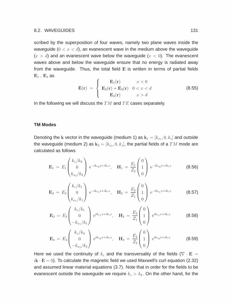
8.2. WAVEGUIDES 131
scribed by the superposition of four waves, namely two plane waves inside the
waveguide (0 < x < d), an evanescent wave in the medium above the waveguide
(x > d) and an evanescent wave below the waveguide (x < 0). The evanescent
waves above and below the waveguide ensure that no energy is radiated away
from the waveguide. Thus, the total field E is written in terms of partial fields
E1 ..E4 as
E(r) =
E1(r) x < 0
E2(r) + E2(r) 0 < x < d
E4(r) x > d
(8.55)
In the following we will discuss the TM and TE cases separately.
TM Modes
Denoting the k vector in the waveguide (medium 1) as k1 = [kx1, 0, kz] and outside
the waveguide (medium 2) as k2 = [kx2, 0, kz], the partial fields of a TM mode are
calculated as follows
E1 = E1
kz/k2
0
kx2/k2
e−ikx2x+ikzz, H1 =
E1
Z2
0
1
0
e−ikx2x+ikzz (8.56)
E2 = E2
kz/k1
0
kx1/k1
e−ikx1x+ikzz, H2 =
E2
Z1
0
1
0
e−ikx1x+ikzz (8.57)
E3 = E3
kz/k1
0
−kx1/k1
eikx1x+ikzz, H3 =
E3
Z1
0
1
0
eikx1x+ikzz (8.58)
E4 = E4
kz/k2
0
−kx2/k2
eikx2x+ikzz, H4 =
E4
Z2
0
1
0
eikx2x+ikzz (8.59)
Here we used the continuity of kz and the transversality of the fields (∇ · E =
ik · E = 0). To calculate the magnetic field we used Maxwell’s curl equation (2.32)
and assumed linear material equations (3.7). Note that in order for the fields to be
evanescent outside the waveguide we require kz > k2. On the other hand, for the

132 CHAPTER 8. WAVEGUIDES AND RESONATORS
fields to be propagating inside the waveguide we require kz < k2. Thus, waveguide
modes will exist only in the interval k2 < kz < k1.
Having defined the partial fields we know have to match them at the boundaries
x = 0 and x = d. The continuity of the parallel components of electric and magnetic
fields lead to
kx2/k2 −kx1/k1 kx1/k1 0
1/Z2 −1/Z1 −1/Z1 0
0 kx1/k1 exp[−ikx1d] −kx1/k1 exp[ikx1d] kx2/k2 exp[ikx2d]
0 1/Z1 exp[−ikx1d] 1/Z1 exp[ikx1d] −1/Z2 exp[ikx2d]
E1
E2
E3
E4
= 0
(8.60)
This is a homogeneous system of linear equations, that is, an eigenvalue problem.
The reason why we end up with a homogeneous system of equations is the ab-
sence of an excitation, which means that there are no sources or incident fields.
Thus, we are looking for solutions that the system supports in absence of an ex-
ternal driving force, similar to an undriven harmonic oscillator. A homogeneous
system of equations has solutions only if the determinant of the matrix acting on
the eigenvector [E1, E2, E3, E4]T vanishes, that is,
∣
∣
∣
∣
∣
∣
∣
∣
∣
kx2/k2 −kx1/k1 kx1/k1 0
1/Z2 −1/Z1 −1/Z1 0
0 kx1/k1 exp[−ikx1d] −kx1/k1 exp[ikx1d] kx2/k2 exp[ikx2d]
0 1/Z1 exp[−ikx1d] 1/Z1 exp[ikx1d] −1/Z2 exp[ikx2d]
∣
∣
∣
∣
∣
∣
∣
∣
∣
= 0 (8.61)
Writing out the expression for the determinant and arranging terms we obtain
1 +(Z2kx2/k2 − Z1kx1/k1)
(Z2kx2/k2 + Z1kx1/k1)
(Z1 kx1/k1 − Z2kx2/k2)
(Z1kx1/k1 + Z2kx2/k2)exp[2ikx1d] = 0 , (8.62)
which can be written in the form
1 + rpab(kz) r
pbc(kz) e2ikx1d = 0 (8.63)
Here, rpab and rp
bc are the Fresnel reflection coefficients for p polarization, as de-
fined in Eq. (4.39). The subscript ‘ab’ indicates that the reflection is measured
between the upper medium (medium a in Fig. 8.7) and the waveguide (medium
b in Fig. 8.7). Similarly, the subscript ‘bc’ is the reflection coefficient measured

8.2. WAVEGUIDES 133
between the waveguide and the lower medium (medium 3 in Fig. 8.7). Note that
kx1 =√
k21 − k2
z =
√
ω2
c2µ1ε1 − k2
z , kx2 =√
k22 − k2
z =
√
ω2
c2µ2ε2 − k2
z , (8.64)
and hence Eq. (8.63) defines the characteristic equation for the eigenvalues kz.
Every solution for kz defines a waveguide mode. It has to be emphasized that the
sign of the square roots in the expressions for kx1 and kx2 has to be chosen such
that the imaginary part is positive. This ensures that the fields decay exponentially
with distance from the waveguide (evanescent fields). The other sign would imply
an exponential increase, which would violate energy conservation.
TE Modes
A similar analysis can be applied for TE polarized fields, for which the electric field
is parallel to the boundaries. The resulting characteristic equation for kz is
1 + rsab(kz) r
sbc(kz) e2ikx1d = 0 (8.65)
TE1 TE
2 TE3 TE
4
TE5
0
1.1
1.2
1.5
1.3
1.4
kz / k
2
0 0.5 1.0 1.5 2.0
d / λ
TM1
TM2
TM3 TM
4
Figure 8.8: Mode structure of a dielectric slab waveguide with n1 = 1.5 (glass) and
n2 = 1 (air). The vertical axis shows the real part of the normalized propagation
constant kz. There is no cut-off for the fundamental modes TM1 and TE1.

134 CHAPTER 8. WAVEGUIDES AND RESONATORS
with rpab and rp
bc being the Fresnel reflection coefficients for s polarization.
As shown in Fig. 8.8, the mode structure for the dielectric waveguide is similar
to the mode structure of a parallel-plate waveguide in Fig. 8.4. However, due to
the different Fresnel reflection coefficients for TE and TM modes, the curves for
TM and TE modes are no longer the same and split into separate curves. The
fundamental modes TE1 and TM1 have no cut-off and in the limit d/λ → 0 they
become plane waves (kz = k2). Similarly, in the limit d/λ→ ∞ the modes become
plane waves propagating in the higher dielectric (kz = k1).
8.2.4 Optical Fibers
In many regards the mode structure in optical fibers is similar to the mode structure
of a dielectric slab waveguide. There are, however, also some relevant differences.
First, an optical fiber is a waveguide that confines the electromagnetic field in two
dimensions which, according to Section 8.2.2, leads to two mode indices nm. One
of them specifies the angular dependence of the fields [sinmφ, cosmφ] and the
other one the radial dependence [Jn(ρ), H(1)n (ρ)]. Second, besides pure TE and
0
1
2
5
3
4
atte
nu
atio
n (
dB
/ k
m)
0.7 0.9 1.1 1.5 1.7
wavelength (μm)
1.3
Figure 8.9: Attenuation in an optical fiber. Lowest propagation losses are obtained
at wavelengths of ∼ 1.3µm and ∼ 1.5µm.

8.2. WAVEGUIDES 135
TM modes there are also hybrid modes, which are classified as HE and EH
modes. HE modes have TE flavor whereas the EH modes have more TM char-
acter.
There are two basic versions of optical fibers: gradient index fibers and step-
index fibers. The former has an index of refraction profile that varies gradually
with radius [n = n(ρ)], whereas the latter exhibits an abrupt transitions between
two refractive indices, similar to the slab waveguide. Step-index fibers are the
most commonly used fibers and usually the index difference is very small, that is
(n1 − n2)/n1 ≪ 1, which is referred to as the weakly guiding condition. Polarized
weakly guided modes are denoted as LPnm modes. A single-mode fiber supports
only the fundamental LP01 mode and all higher-order modes are suppressed by
the cut-off condition. Fig. 8.9 shows the propagation loss in a modern optical fiber.
The losses on the short-wavelength side are due to Rayleigh scattering and the
losses at the long wavelength end are due to infrared absorption. The bumps are
absorption bands of molecular bonds, such as OH−. The lowest attenuation is
obtained near 1.3 and 1.5 µm and is the reason why fiber-optic communication is
operated at these wavelengths.

136 CHAPTER 8. WAVEGUIDES AND RESONATORS

Chapter 9
Classical Electron Theory
137

138 CHAPTER 9. CLASSICAL ELECTRON THEORY

Chapter 10
Coherence Theory
139

140 CHAPTER 10. COHERENCE THEORY

Chapter 11
Relativistic Electromagnetics
141

142 CHAPTER 11. RELATIVISTIC ELECTROMAGNETICS

Chapter 12
Antennas
143


