1

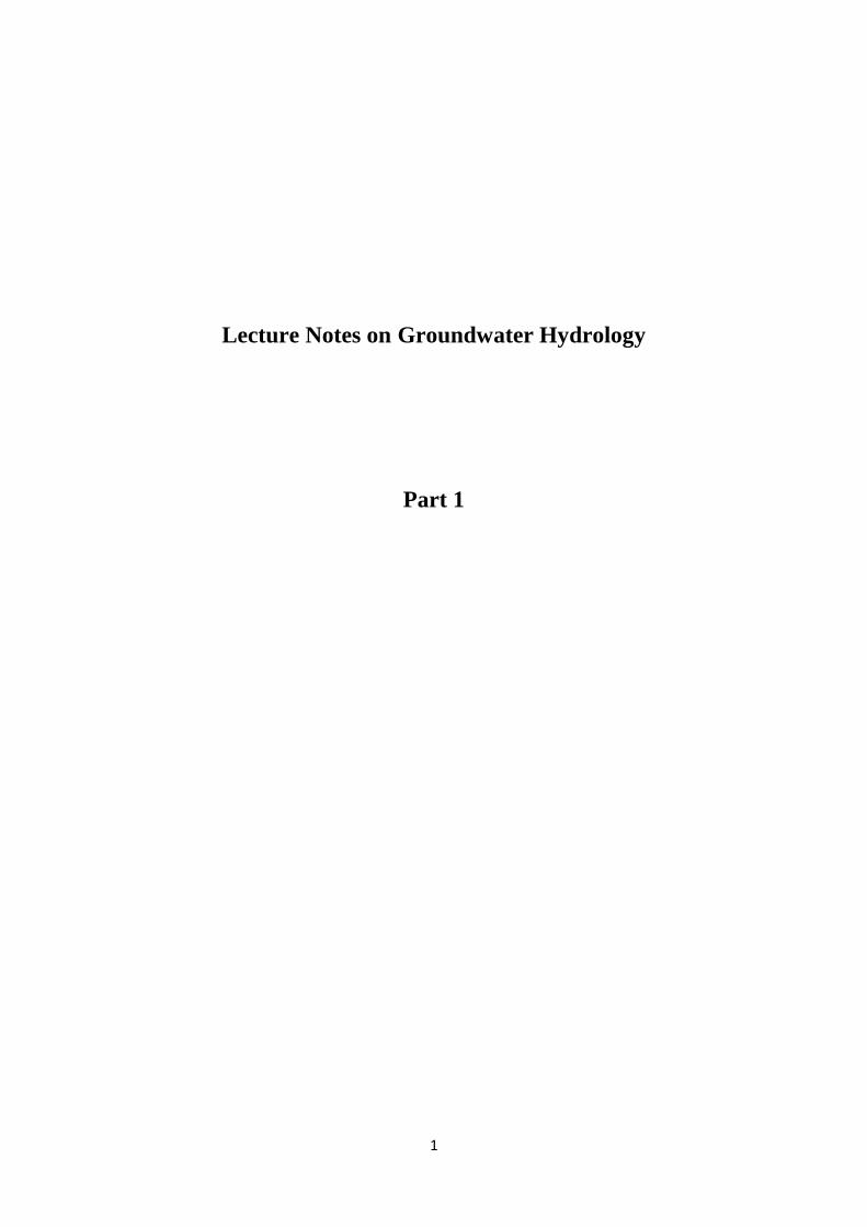
Lecture Notes on Groundwater Hydrology

Part 1

2

1. Basic concepts and definitions

1.1 Aquifer, Aquitard, Aquiclude and Aquifuge

Aquifer is a word produced from two Latin words: Aqua, which means water and ferre,

which means to bear. Therefore, the term Aquifer can literally be understood as Water-

bearing formation.

Aquifer can formally be defined as a saturated permeable geological unit that is permeable

enough to yield economic quantities of water to wells. In other words, it is defined as a satu-

rated geological unit that can transmit significant quantities of water under hydraulic head.

The most important underground water-bearing materials are unconsolidated sand and grav-

els. But, permeable sedimentary rocks such as sandstone and limestone, and heavily fractured

or weathered volcanic and crystalline rocks can also be taken as aquifer (water-bearing) mate-

rials.

Aquitard is a geological unit that is permeable enough to transmit water in significant quanti-

ties for large area and long period. But, its permeability is not sufficient to justify the con-

struction of production wells to be placed in it. In other words, Aquitard is a geologic for-

mation that can transmit water at a relatively lower rate compared to aquifer. Example in-

cludes formations that are predominantly clays, loams and shales.

Aquiclude is an impermeable geological unit which does not transmit water at all. Although

this formation is capable of absorbing water slowly. It means that this geological formation

can store water, but cannot transmit it easily. In other words, Aquiclude is a saturated geolog-

ical unit that is incapable of transmitting significant quantities of water under ordinary hy-

draulic head. Example: metamorphic rocks.

Aquifuge is a geological formation that can neither absorbs nor transmits water.

1.2 Types of Aquifer

There are three types of aquifer: confined, unconfined and leaky and their definition is given

as follows.

1.2.1 Confined aquifer

3

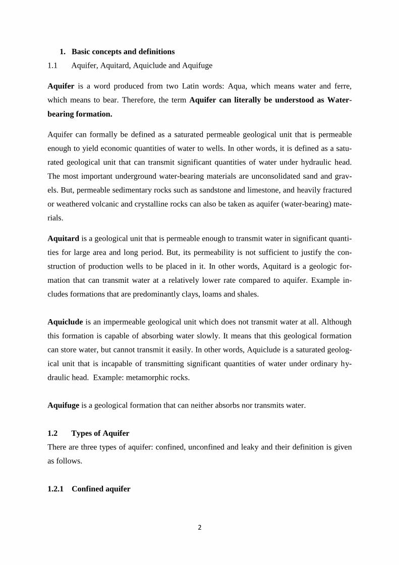
A confined aquifer is an aquifer which is bounded by an aquiclude both at the lower and up-

per part. In other words, this aquifer is confined between two impervious layers. The con-

fined aquifer is known as pressure aquifer. In a confined aquifer, the pressure of water is

higher than atmospheric pressure. The water in a well which is constructed in such an aquifer

rises usually above the aquifer and even above the ground surface due to high pressure. By the

way, the groundwater pressure can be either equal or greater than atmospheric pressure. Con-

fined aquifer cannot be recharged directly by infiltration.

Figure 1 Confined Aquifer.

4

1.2.2 Unconfined aquifer

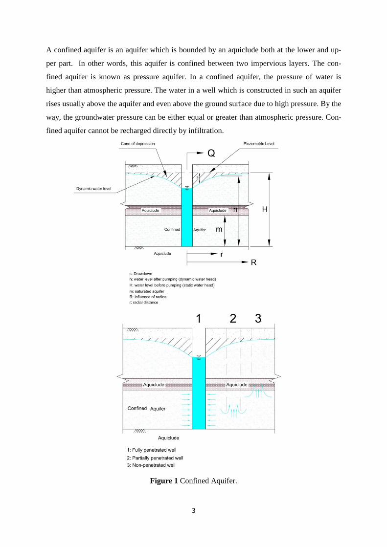
An unconfined aquifer is an aquifer which is bounded by aquiclude at its lower side and by

water table at its upper side. In other words, the flow of water in the upper part of the aquifer

is not restricted by any confining layer and that makes the upperpart a bounded free surface.

Consequently, the free surface of unconfined aquifer is under atmospheric pressure. Its upper

boundary is watertable which is free to rise and fall. Unconfined aquifer is directly recharged

by infiltration.

Figure 2 Unconfined Aquifer.

5

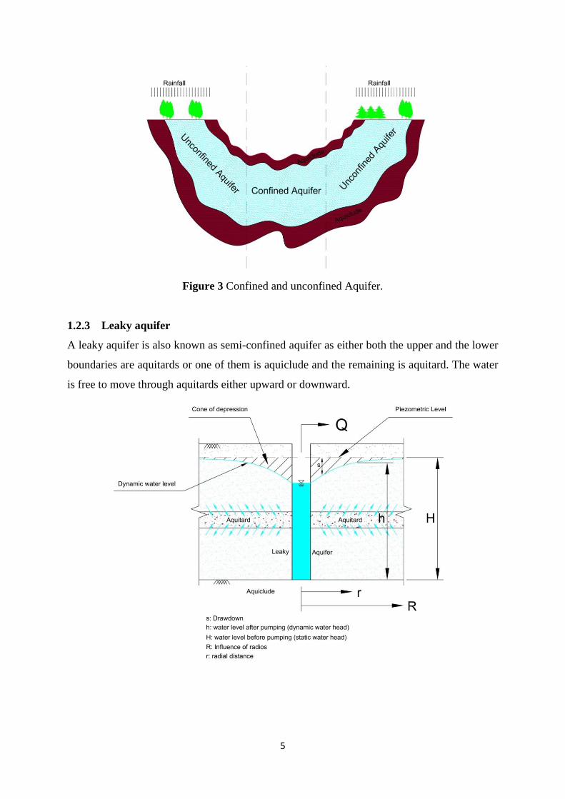
Figure 3 Confined and unconfined Aquifer.

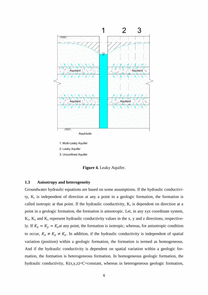
1.2.3 Leaky aquifer

A leaky aquifer is also known as semi-confined aquifer as either both the upper and the lower

boundaries are aquitards or one of them is aquiclude and the remaining is aquitard. The water

is free to move through aquitards either upward or downward.

6

Figure 4. Leaky Aquifer.

1.3 Anisotropy and heterogeneity

Groundwater hydraulic equations are based on some assumptions. If the hydraulic conductivi-

ty, K, is independent of direction at any a point in a geologic formation, the formation is

called isotropic at that point. If the hydraulic conductivity, K, is dependent on direction at a

point in a geologic formation, the formation is anisotropic. Let, in any xyz coordinate system,

Kx, Ky and Kz represent hydraulic conductivity values in the x, y and z directions, respective-

ly. If 𝐾𝑥 = 𝐾𝑦 = 𝐾𝑧at any point, the formation is isotropic, whereas, for anisotropic condition

to occur, 𝐾𝑥 ≠ 𝐾𝑦 ≠ 𝐾𝑧. In addition, if the hydraulic conductivity is independent of spatial

variation (position) within a geologic formation, the formation is termed as homogeneous.

And if the hydraulic conductivity is dependent on spatial variation within a geologic for-

mation, the formation is heterogeneous formation. In homogeneous geologic formation, the

hydraulic conductivity, K(x,y,z)=C=constant, whereas in heterogeneous geologic formation,

7

the hydraulic conductivity, K(x,y,z)≠C. We can say that aquifers and aquitards are homoge-

nies and isotropic if we assume that the hydraulic conductivity is same throughout a geologic

formation and in all directions. If hydraulic conductivity in the horizontal direction Kh is

greater than the hydraulic conductivity in the vertical direction Kv, this phenomenon is called

anisotropy. In fact, lithology of geological formation varies significantly horizontally and ver-

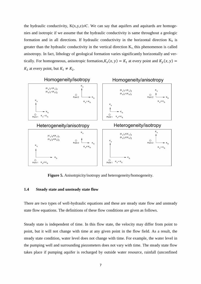
tically. For homogeneous, anisotropic formation,𝐾𝑥(𝑥, 𝑦) = 𝐾1 at every point and 𝐾𝑦(𝑥, 𝑦) =

𝐾2 at every point, but 𝐾1 ≠ 𝐾2.

Figure 5. Anisotrpicity/isotropy and heterogeneity/homogeneity.

1.4 Steady state and unsteady state flow

There are two types of well-hydraulic equations and these are steady state flow and unsteady

state flow equations. The definitions of these flow conditions are given as follows.

Steady state is independent of time. In this flow state, the velocity may differ from point to

point, but it will not change with time at any given point in the flow field. As a result, the

steady state condition, water level does not change with time. For example, the water level in

the pumping well and surrounding piezometers does not vary with time. The steady state flow

takes place if pumping aquifer is recharged by outside water resource, rainfall (unconfined

8

aquifer), leakage through the aquitard (Leaky aquifer) from upward or downward and directly

from open water sources. As a result, we can say that steady state flow is attained if the

changes in the water level in wells and piezometers are very small with time that they can be

ignored.

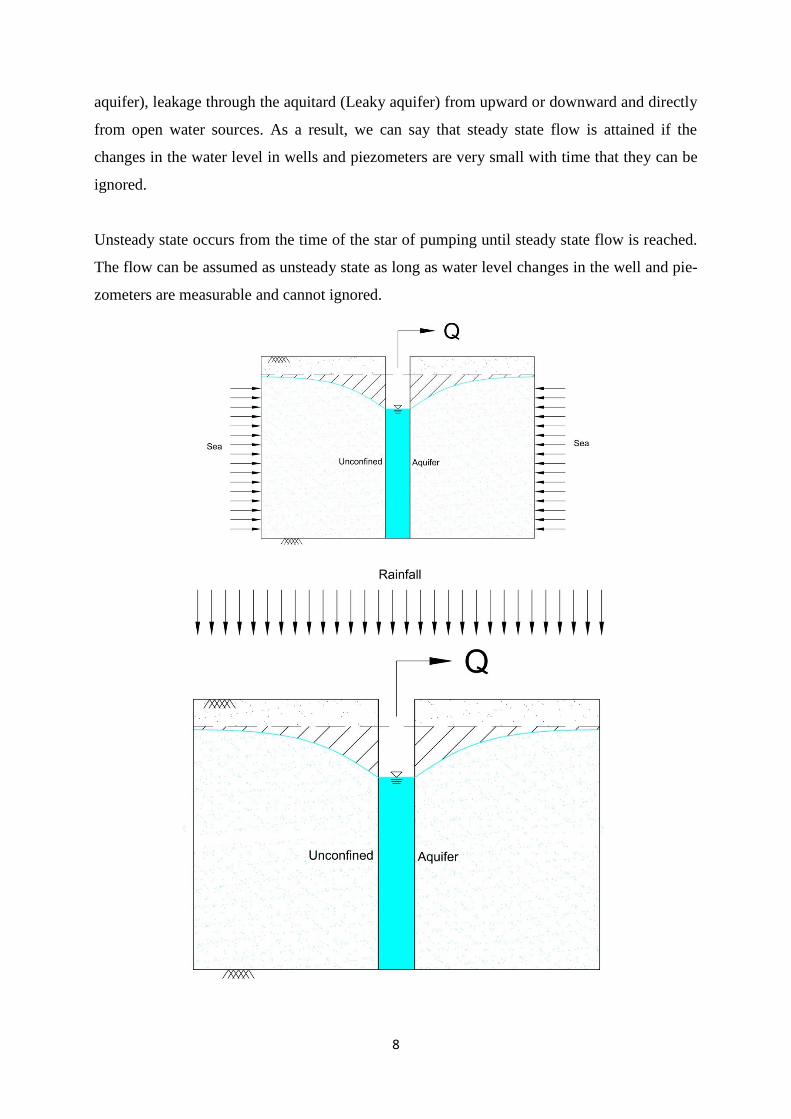
Unsteady state occurs from the time of the star of pumping until steady state flow is reached.

The flow can be assumed as unsteady state as long as water level changes in the well and pie-

zometers are measurable and cannot ignored.

9

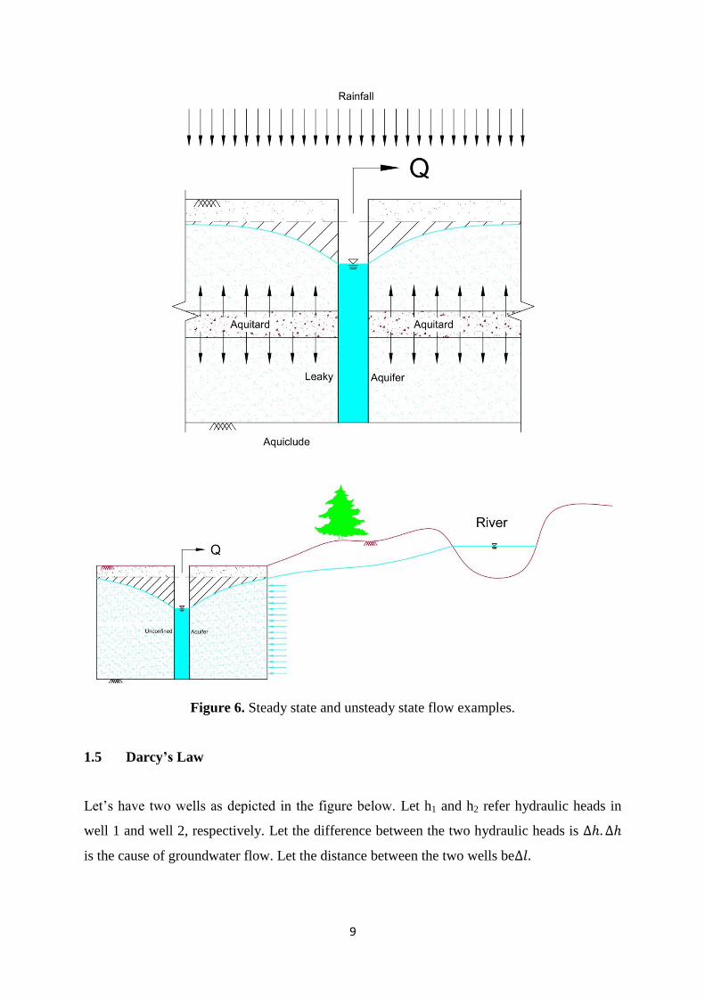
Figure 6. Steady state and unsteady state flow examples.

1.5 Darcy’s Law

Let’s have two wells as depicted in the figure below. Let h1 and h2 refer hydraulic heads in

well 1 and well 2, respectively. Let the difference between the two hydraulic heads is ∆ℎ. ∆ℎ

is the cause of groundwater flow. Let the distance between the two wells be∆𝑙.

10

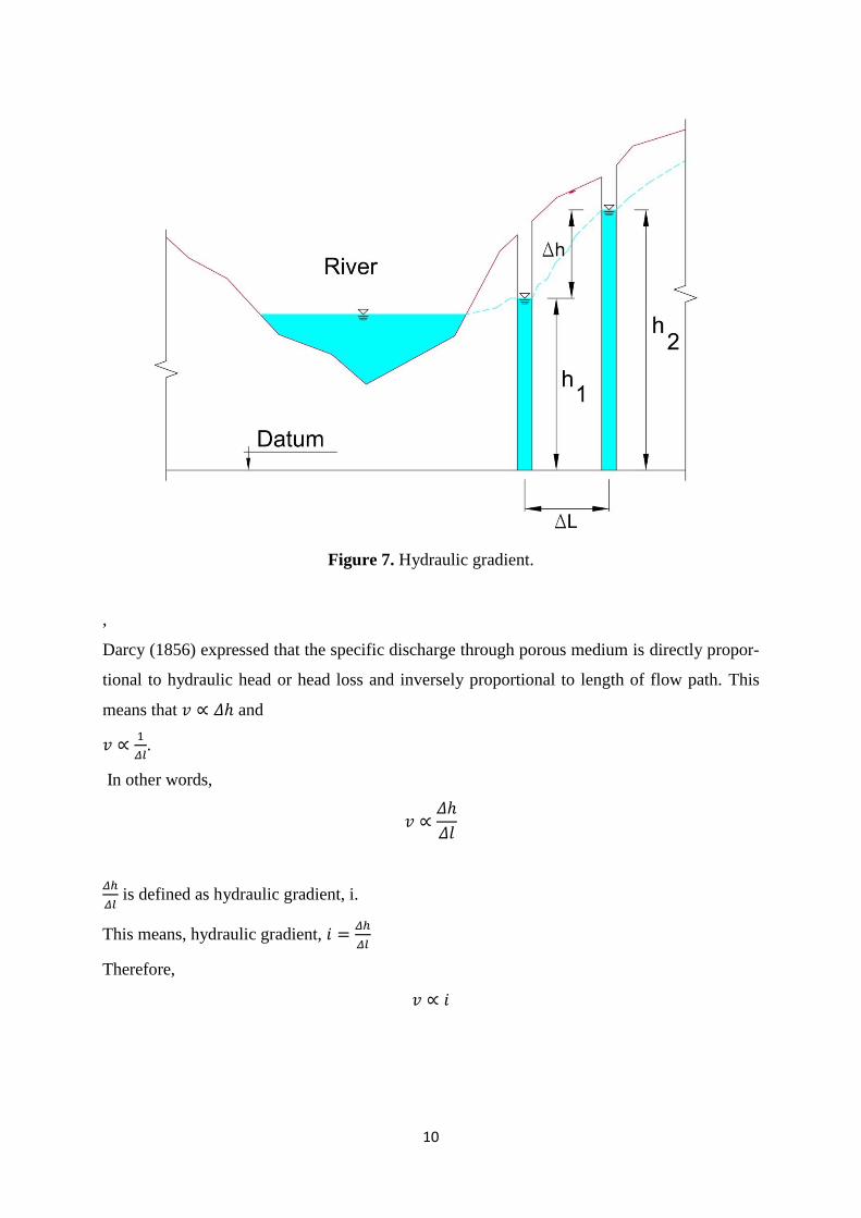
Figure 7. Hydraulic gradient.

,

Darcy (1856) expressed that the specific discharge through porous medium is directly propor-

tional to hydraulic head or head loss and inversely proportional to length of flow path. This

means that 𝑣 ∝ 𝛥ℎ and

𝑣 ∝1

𝛥𝑙.

In other words,

𝑣 ∝𝛥ℎ

𝛥𝑙

𝛥ℎ

𝛥𝑙 is defined as hydraulic gradient, i.

This means, hydraulic gradient, 𝑖 =𝛥ℎ

𝛥𝑙

Therefore,

𝑣 ∝ 𝑖

11

This proportionality is converted to equality by introducing a constant coefficient, K that has

logical physical meaning. This coefficient depends on the characteristics of the porous medi-

um and the groundwater. It refers to a resistance coefficient and is called hydraulic conductiv-

ity.

This can be written mathematically as:

𝑣 = 𝑘𝛥ℎ

𝛥𝑟 (1)

or in differential form

𝑣 = 𝑘𝑑ℎ

𝑑𝑙 (2)

This is what is known as Darcy’s Law.

Here 𝑣 =𝑄

𝐴 is specific discharge (also known as Darcy velocity or Darcy flux (Length/time)),

Q= volume rate of flow (Length3/time), A=cross-sectional area normal to flow direction, Δh=

head loss which is the difference between hydraulic heads measured at points 1 and 2

(Length), Δl= the distance between the two wells as indicated earlier. As defined above,

𝑑ℎ

𝑑𝑙= 𝑖, is hydraulic gradient (dimensionless) and k is proportionality constant which is termed

as hydraulic conductivity (Length/Time).

In geotechnical engineering, permeability is used in place of hydraulic conductivity. Hydrau-

lic conductivity is a property of both the fluid and the porous medium, whereas permeability

depends only on the property of the porous medium.

We have to know that Darcy Law has its range of validity. Darcy’s Law is valid for laminar

flow, but not for turbulent flow. Turbulent flow can happen in cavernous limestone and frac-

tured basalt. In case of doubt, we can use Reynolds number in order to determine whether a

flow is laminar or turbulent flow. The Reynolds number is described as the ratio of inertial

forces to viscous forces, and is given as:

𝑅𝑒 =𝜌.𝑣.𝑑

𝜇

Here, ρ is the specific mass of fluid, v is specific discharge, μ is dynamic viscosity of fluid

and d is a representative length of porous medium which is a mean grain diameter (Length) or

a mean pore diameter. If d increases, the value of Reynolds number increases, affecting the

flow regime.

12

Darcy concluded that the law’s range of validity is between 1<Re<10. Re=10 is upper limit of

the validity of Darcy’s flow. Most ground water flow occur when Re number is less than 1.

Therefore, Darcy’s Law applies in ground water flow conditions. Exceptional situations are

rock wide opening, vicinity of pumped well and where steep hydraulic head exists. Darcy’s

Law is invalid at low hydraulic gradient. Consequently, Darcy’s low is valid if the Reynolds

number stays in range from 1 to 10. All flow through granular media is laminar.

Darcy’s Experiment

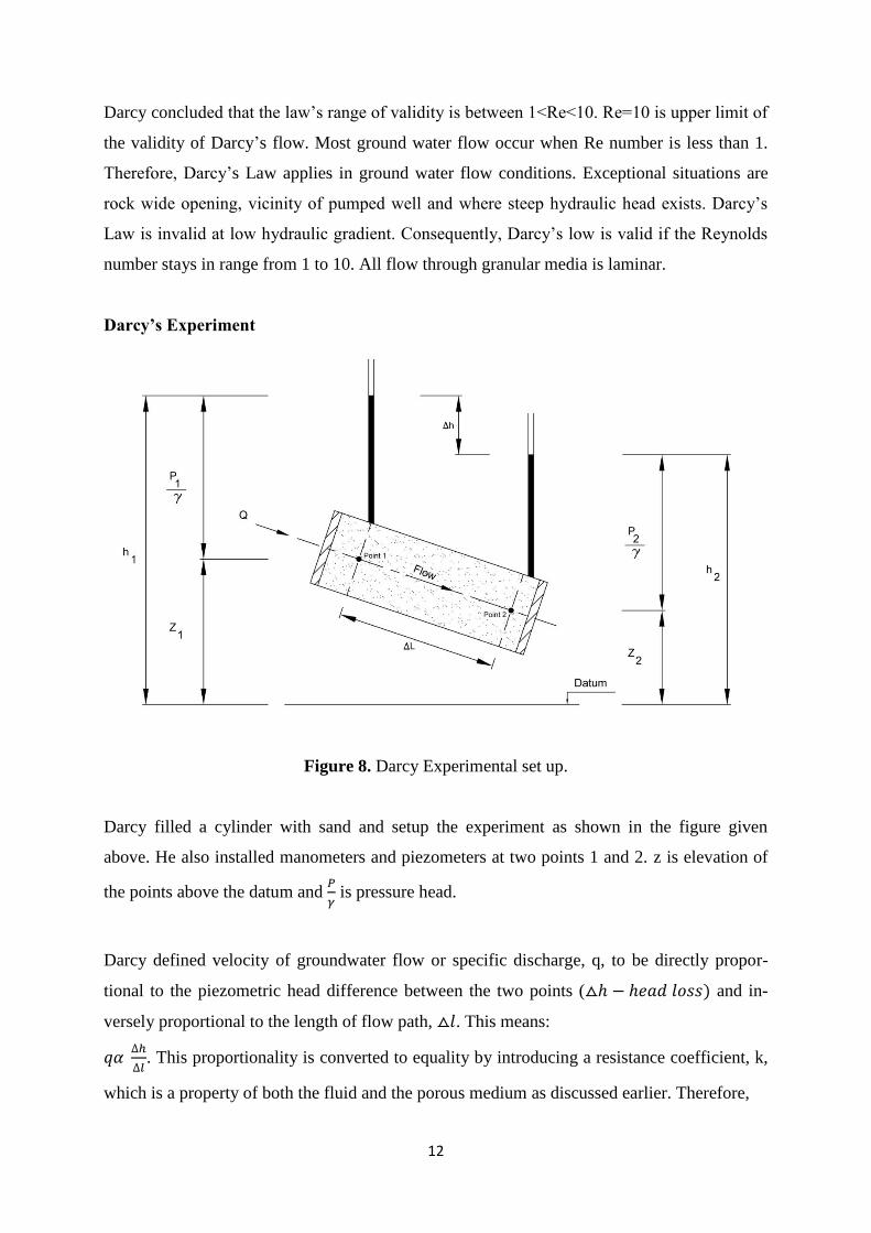
Figure 8. Darcy Experimental set up.

Darcy filled a cylinder with sand and setup the experiment as shown in the figure given

above. He also installed manometers and piezometers at two points 1 and 2. z is elevation of

the points above the datum and 𝑃

𝛾 is pressure head.

Darcy defined velocity of groundwater flow or specific discharge, q, to be directly propor-

tional to the piezometric head difference between the two points (⧍ℎ − ℎ𝑒𝑎𝑑 𝑙𝑜𝑠𝑠) and in-

versely proportional to the length of flow path, ⧍𝑙. This means:

𝑞𝛼 ∆ℎ

∆𝑙. This proportionality is converted to equality by introducing a resistance coefficient, k,

which is a property of both the fluid and the porous medium as discussed earlier. Therefore,

13

𝑞 = 𝑘∆ℎ

∆𝑙

Since ∆ℎ

∆𝑙= 𝑖 (hydraulic gradient) then, 𝑞 = 𝑘𝑖

The differential form of the equation is given as 𝑞 = −𝑘𝑑ℎ

𝑑𝑙

Negative sign is put in front because the difference between piezometric head 2 and piezomet-

ric head 1 is negative. We should multiply the value by negative so that the specific discharge

will be positive with a physical meaning.

In addition, we know that

𝑠 + ℎ = 𝐻

,where s is drawdown, h is hydraulic head and H is static water level.

In differential form, the equation can be rewritten as:

𝑑𝑠 + 𝑑ℎ = 𝑑𝐻

Dividing both sides of the equation by the differential distance, dr, yields:

𝑑𝑠

𝑑𝑟+

𝑑ℎ

𝑑𝑟=

𝑑𝐻

𝑑𝑟

But,𝑑𝐻

𝑑𝑟 is zero as H is constant.

Therefore,

𝑑𝑠

𝑑𝑟+

𝑑ℎ

𝑑𝑟= 0

This implies that

𝑑𝑠

𝑑𝑟= −

𝑑ℎ

𝑑𝑟

Bernoulli’s Equation can be used to drive Darcy’s Equation. Bernoulli’s Eq. states that, at any

point in a flow field, the sum of elevation head (Z), pressure head (𝑃

𝛾) and velocity head (

𝑣2

2𝑔)

remain constant. This means:

𝑍1 +𝑃1

𝛾 +

𝑣12

2𝑔= 𝑍2 +

𝑃2

𝛾 +

𝑣22

2𝑔+ ⧍ℎ

,where ⧍h is head loss as a result of friction.

14

Since the flow in porous medium, groundwater flow being one of a kind, is very slow, the

velocity head in the above equation can be ignored. Therefore,

𝑍1 +𝑃1

𝛾 = 𝑍2 +

𝑃2

𝛾+ ⧍ℎ

Rearranging this equation, we can find the following equation.

(𝑍1 +𝑃1

𝛾) − (𝑍2 +

𝑃2

𝛾) = ⧍ℎ

We know that (𝑍1 +𝑃1

𝛾) and (𝑍2 +

𝑃2

𝛾) are piezometric heads, ℎ2and ℎ2, respectively.

Therefore, Eq. x can be written as

(ℎ1 − ℎ2) = ⧍ℎ

Dividing both sides of Eq. x by ⧍𝑙, where ⧍𝑙 is the distance between the two points of inter-

est, we will find:

(𝑍1+𝑃1𝛾

)

∆𝑙−

(𝑍2+𝑃2𝛾

)

∆𝑙=

⧍ℎ

∆𝑙

We know, from earlier definition that ⧍ℎ

∆𝑙 is hydraulic gradient.

Based on the definition given by Darcy, as written above, this hydraulic gradient is propor-

tional to velocity of groundwater flow or specific discharge, q.

This means that∆ℎ

∆𝑙𝛼 𝑞.

Following the same logic given earlier, this proportionality is converted to equality by intro-

ducing a resistance coefficient, k, which is a property of both the fluid and the porous medi-

um. Therefore,

𝑞 = 𝑘∆ℎ

∆𝑙

1.6 Hydraulic head and Fluid potential

It is known that heat flows through solids from higher to lower values of temperature. Electri-

cal current flows through electrical circuits from higher voltage to lower voltage value. Tem-

15

perature and voltage are potential quantities, and the rates of flows of heat and electricity are

proportional to temperature gradient and voltage gradient, respectively. In the same manner,

the fluid potential, which is responsible for flow through porous media is mechanical energy

per unit mass of fluid.

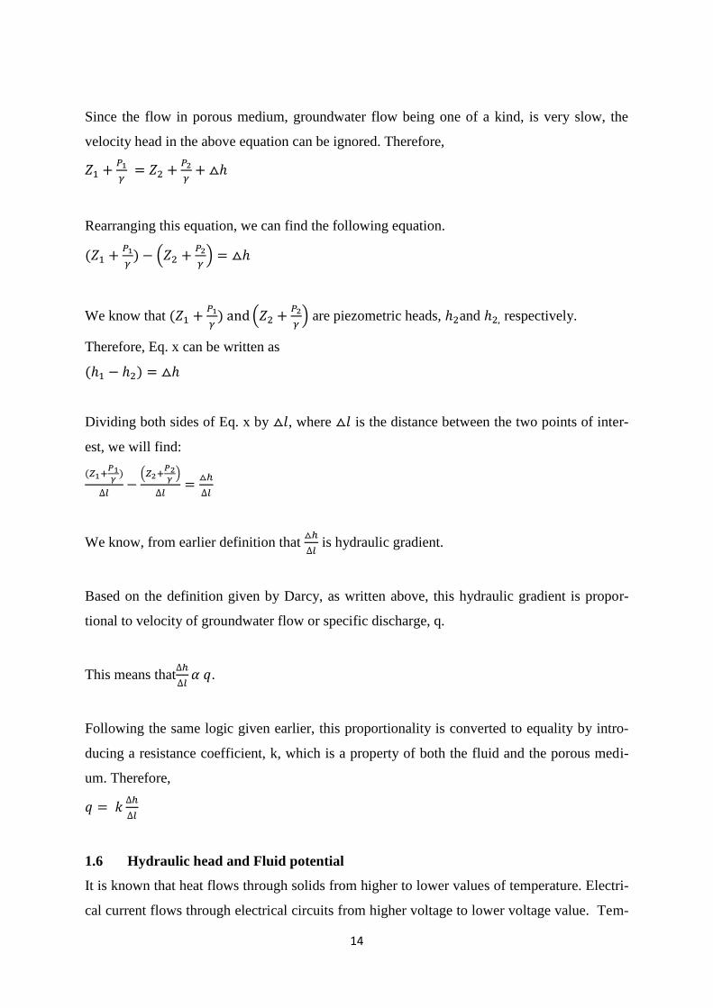
If we consider a particle in a flow, work is required to lift the particle from the datum to a

certain elevation as depicted in the figure below.

Figure 9. Particle position.

There are three required components of the work to be calculated. First, there is work required

to lift the mass from elevation, z=0 from elevation=z.

𝑤1 = 𝑚𝑔𝑧

Second, there is work required to accelerate the fluid from velocity, v=0 to velocity, v.

𝑤2 =1

2𝑚𝑣2

Third, there is work required to rise the pressure from p=po=atmospheric to pressure, p.

𝑤3 = 𝑚 ∫𝑑𝑝

𝜌

𝑝

𝑝0

The total mechanical energy per unit mass is the sum of these three components of work. For

a unit mass of fluid, m=1. The total mechanical energy can, therefore, be written as:

𝑤 = 𝑔𝑧 +1

2𝑣2 + ∫

𝑑𝑝

𝜌

𝑝

𝑝𝑜

After mathematical processing,

𝑤 = 𝑔𝑧 +1

2𝑣2 +

𝑝−𝑝𝑜

𝜌

16

We know that the velocity of groundwater flow is extremely low. Therefore, the second term

of the right hand side of the above equation can be ignored. By the way, fluids are incom-

pressible. This means that specific mass is constant and does not change with pressure.

The equation can, therefore, be simplified as:

𝑤 = 𝑔𝑧 +𝑝−𝑝𝑜

𝜌

As can be seen in the above equation, the first term in the right hand side of the equation in-

volves elevation and second term involves pressure term.

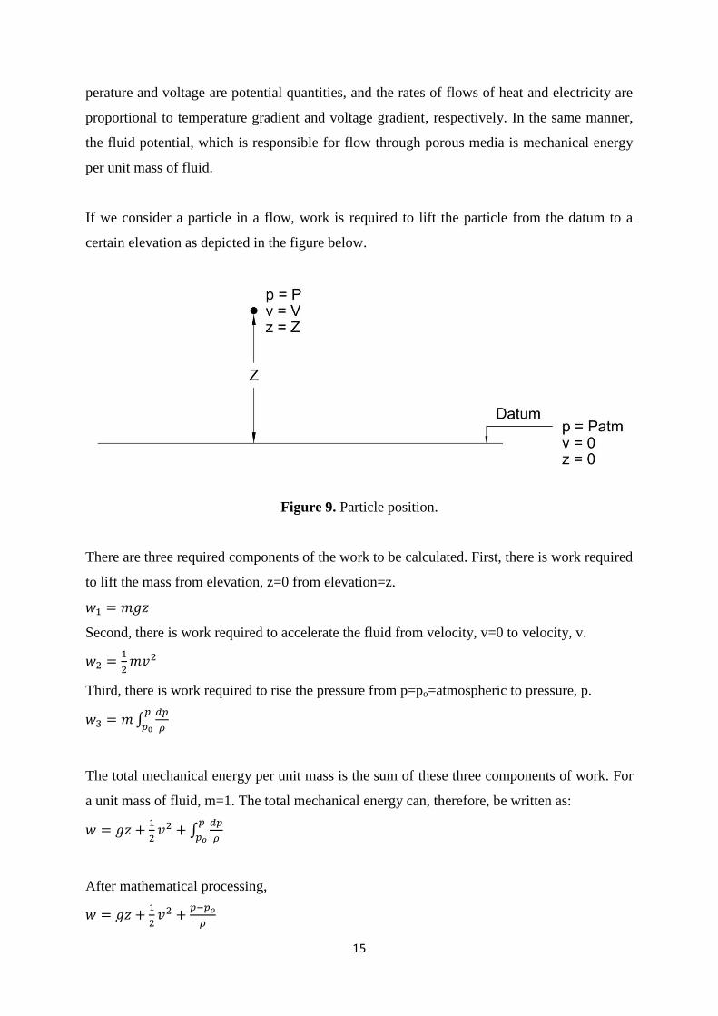
How can we relate these terms to hydraulic head, h. Let’s think about Darcy manometer.

Figure 10. Piezometer.

The pressure at the manometer located at point1 is expressed as:

𝑝 = 𝑝𝑜 + 𝜌𝑔 𝜓

Here, po is atmospheric pressure and ψ is height of fluid column, which is equal to (h-z).

After algebraic manipulation,

𝑝 − 𝑝0 = 𝜌𝑔(ℎ − 𝑧)

17

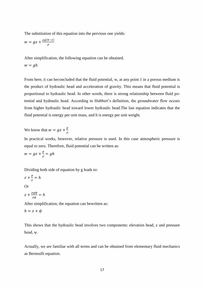
The substitution of this equation into the pervious one yields:

𝑤 = 𝑔𝑧 +𝜌𝑔(ℎ−𝑧)

𝜌

After simplification, the following equation can be obtained.

𝑤 = 𝑔ℎ

From here, it can beconcluded that the fluid potential, w, at any point 1 in a porous medium is

the product of hydraulic head and acceleration of gravity. This means that fluid potential is

proportional to hydraulic head. In other words, there is strong relationship between fluid po-

tential and hydraulic head. According to Hubbert’s definition, the groundwater flow occurs

from higher hydraulic head toward lower hydraulic head.The last equation indicates that the

fluid potential is energy per unit mass, and h is energy per unit weight.

We know that 𝑤 = 𝑔𝑧 +𝑝

𝜌

In practical works, however, relative pressure is used. In this case atmospheric pressure is

equal to zero. Therefore, fluid potential can be written as:

𝑤 = 𝑔𝑧 +𝑝

𝜌= 𝑔ℎ

Dividing both side of equation by g leads to:

𝑧 +𝑝

𝛾= ℎ

Or

𝑧 +𝜌𝑔𝜓

𝜌𝑔= ℎ

After simplification, the equation can bewritten as:

ℎ = 𝑧 + 𝜓

This shows that the hydraulic head involves two components: elevation head, z and pressure

head, ψ.

Actually, we are familiar with all terms and can be obtained from elementary fluid mechanics

as Bernoulli equation.

18

We can write concepts of fluid potential and hydraulic head in terms of Bernoulli’s equation.

The total head is given as:

ℎ𝑡 = ℎ𝑧 + ℎ𝑝 + ℎ𝑣

Here hz is elevation head, hp is pressure head and hv is velocity head. Therefore,

ℎ𝑡 = 𝑧 +𝑝

𝛾+

𝑣2

2𝑔

In case of groundwater flow, velocities are extremely low. Because of this, velocity head is

equal to zero, and the above equation becomes:

ℎ = 𝑧 +𝜌𝑔𝜓

𝜌𝑔

After simplification, the equation becomes:

ℎ = 𝑧 + 𝜓

This relationship shows that, if we consider a pipe positioned horizontally, flow occurs as a

result of pressure head, and if we consider vertically positioned pipe, elevation head is re-

sponsible for flow to occur.

Classification of sub-surface

Let’s consider the following figure.

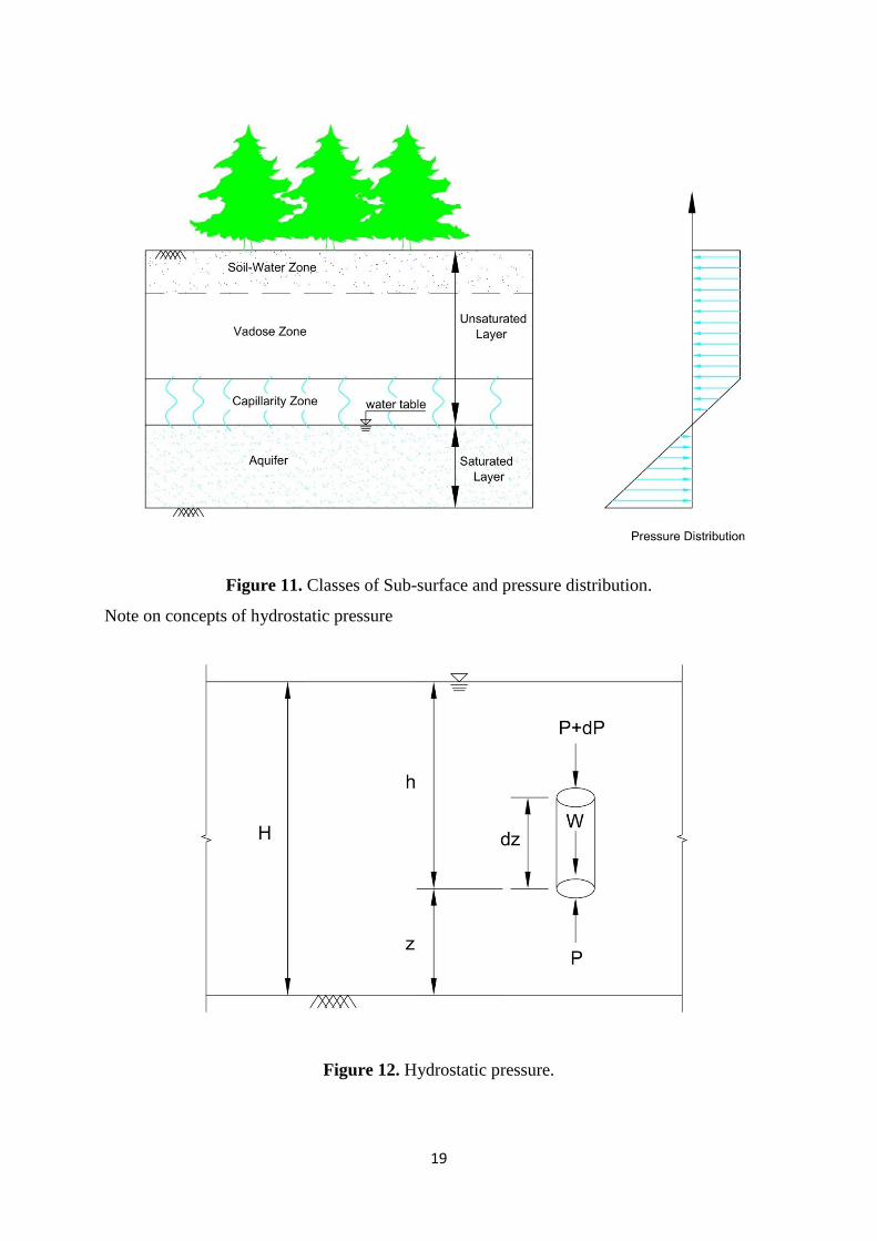
The sub-surface can generally be divided into two zones: Unsaturated zone and saturated

zone. In the unsaturated zone, pore spaces are partially filled by water. However, saturated

zone is a zone where all the void space is filled by water. The boundary between the saturated

and unsaturated zones is called as the water table, which is the surface of the saturated zone,

the fluid pressure at this surface is atmospheric pressure. Unsaturated zone can further be di-

vided into Soil water zone, Vadose zone and Capillary zone.

In the capillary zone, there is a negative pressure (suction), and considering the following

figure, the pressure distribution will have the following form.

19

Figure 11. Classes of Sub-surface and pressure distribution.

Note on concepts of hydrostatic pressure

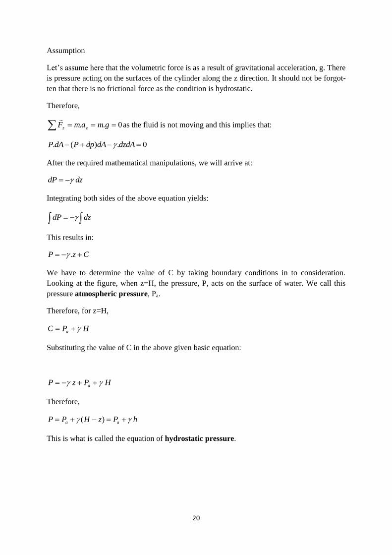
Figure 12. Hydrostatic pressure.

20

Assumption

Let’s assume here that the volumetric force is as a result of gravitational acceleration, g. There

is pressure acting on the surfaces of the cylinder along the z direction. It should not be forgot-

ten that there is no frictional force as the condition is hydrostatic.

Therefore,

0.. gmamF zz

as the fluid is not moving and this implies that:

0.)(. dzdAdAdpPdAP

After the required mathematical manipulations, we will arrive at:

dzdP

Integrating both sides of the above equation yields:

dzdP

This results in:

CzP .

We have to determine the value of C by taking boundary conditions in to consideration.

Looking at the figure, when z=H, the pressure, P, acts on the surface of water. We call this

pressure atmospheric pressure, Pa.

Therefore, for z=H,

HPC a

Substituting the value of C in the above given basic equation:

HPzP a

Therefore,

hPzHPP aa )(

This is what is called the equation of hydrostatic pressure.

21

Important Terminologies

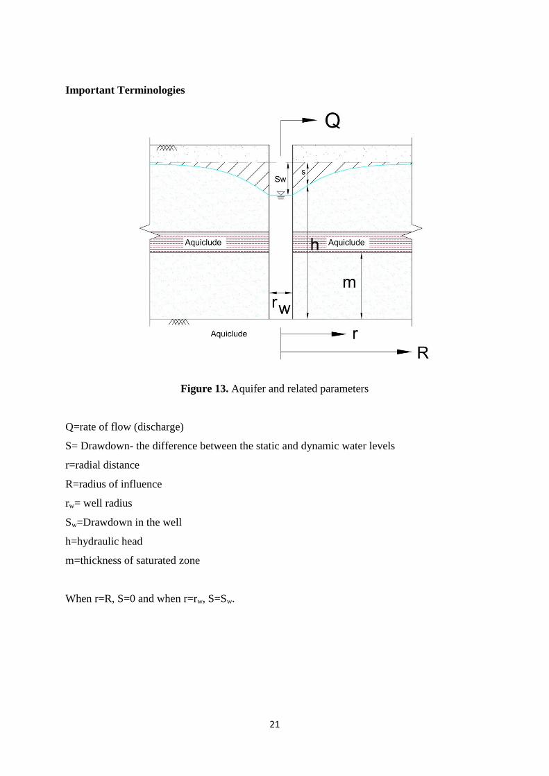
Figure 13. Aquifer and related parameters

Q=rate of flow (discharge)

S= Drawdown- the difference between the static and dynamic water levels

r=radial distance

R=radius of influence

rw= well radius

Sw=Drawdown in the well

h=hydraulic head

m=thickness of saturated zone

When r=R, S=0 and when r=rw, S=Sw.

22

1.7 Physical properties

1.7.1 Porosity (n)

If we consider a certain volume of unconsolidated material, the total unit volume, VT, of the

unconsolidated material can be divided into the volume of its solid portion, Vs, and the vol-

ume of its voids, Vv. The total volume of the unconsolidated material can be written in terms

of the volumes of both solid and void as:

𝑉𝑇 = 𝑉𝑆 + 𝑉𝑣

Let’s divide both of sides of the equation by total volume, VT. This yields:

1 =𝑉𝑠

𝑉𝑇+

𝑉𝑣

𝑉𝑇

The second term in right hand side of this equation represents porosity. It is defined as the

ratio of volume of void space to total volume of rock mass. Porosity is strongly related to void

space.

𝑛 =𝑉𝑣

𝑉𝑇

Porosity is usually expressed as a percentage. The porosity values take in range from 0 to 1

based on geometrical formation. The porosity indicates the capability of the medium to store

water. In other words, it measures water bearing capacity. Therefore, the total potential of

groundwater can be calculated by using the following expression.

𝑉𝑝 = 𝑛 𝑉𝑎

Here Vp is potential of ground water, Va is volume of aquifer.

As a result, porosity is one of the most important parameters in order to determine hydraulic

conductivity. We can evaluate the water potential in the groundwater by porosity if there is no

pressure. Not all the water found in the pore space can be extracted as some of the water will

remain in the void space because of surface tension forces. This makes porosity not to be a

good measure of water that can be extracted. In general, the rocks have lower porosities than

soils, gravels, sands and silts.

1.7.2 Specific yield and retention

As indicated earlier, all of the water found in an aquifer cannot be abstracted from the aquifer

making porosity not to be a good indicator of water potential. Some of the water will be kept

in the void by molecular and surface tension forces. A good indicator of water potential is

23

specific yield. The specific yield can be defined as the ratio of the volume of yielded water to

the total volume of rock mass. The specific yield is also known as effective porosity.

We know that 𝑉𝑣 = 𝑉𝑦 + 𝑉𝑟

Where 𝑉𝑣 is volume of voids, 𝑉𝑦 is volume of water that can be yielded and 𝑉𝑟 is volume of

water retained in the porous medium.

If we divide both sides of the equation by the total volume of the rock mass, 𝑉𝑇, we will find:

𝑉𝑣

𝑉𝑇=

𝑉𝑦

𝑉𝑇+

𝑉𝑟

𝑉𝑇

Obviously, 𝑉𝑣

𝑉𝑇 is porosity,

𝑉𝑦

𝑉𝑇 is called specific yield and

𝑉𝑟

𝑉𝑇 s specific retention.

Therefore, total porosity can be written as

𝑛 = 𝑆𝑦 + 𝑆𝑟

Here Sy is specific yield and Sr is specific retention. Specific yield indicates the amount of

water available to use and it is more important than porosity value.

In general, rocks have lower porosities than soils, gravels, sands and silts. Clays have higher

porosities than sand and gravels, but lower hydraulic conductivities. For example, the porosity

of volcanic rocks is approximately 2 %. But, they yield all water that exists in their voids.

Oppositely, clays have very high porosity values, but they can yield less than 5 % of water

that exists in their voids.

It can be concluded that finer grain sizes have greater specific retention values compared to

coarse-grained materials. Specific yield of aquifer is always less than the porosity. In fine

grained porous formation, specific yield values are significantly different from their porosity

values, whereas, in course grained materials, specific yield and porosity values are very close

to each other. Specific yield can also be defined as the volume of water that unconfined aqui-

fer release from storage per unit surface area of aquifer per unit decline of the hydraulic head.

Specific yield of unconfined aquifer is much higher than storage coefficient of confined aqui-

fer. The specific yield values vary in range from 0.01 through 0.3, which are much higher

than the storativities of confined aquifers. In other words, the specific yield is known as stor-

age coefficient in unconfined aquifer.

Specific yield indicates the quantity of abstracted water and specific retention shows how

much water is retained in the aquifer after the water is yielded by gravity. The specific yield

and specific retention can be written, respectively, as

24

𝑆𝑦 =𝑉𝑦

𝑉𝑇

and

𝑆𝑟 =𝑉𝑟

𝑉𝑇

Here, Vy is volume of yielded water and Vr is volume of retained water. Specific retention

measures the amount of water in the void space against gravity by capillarity and hygroscopic

forces when the hydraulic head in the confined aquifer is declined. This phenomenon is called

specific retention.

1.7.3 Hydraulic conductivity

The hydraulic conductivity is constant of proportionality in Darcy’s law. It is defined as the

volume of water that moves through the porous medium in unit time under a unit hydraulic

gradient. The hydraulic conductivity has dimension of Length/Time (L/T). Hydraulic conduc-

tivity is a function of properties of both the porous medium and fluid. The hydraulic conduc-

tivity is based on the pore and fracture sizes within aquifer. It is well known that horizontal

hydraulic conductivity is approximately three times greater than vertical hydraulic conductivi-

ty based on formation of the porous medium. Hydraulic conductivity and hydraulic head are

used in saturated porous media. Saturated porous media are media where all voids are filled

with water. But, in practice, some of the voids are partially filled with water. This zone is re-

ferred as unsaturated zone.

1.7.4 Permeability

In geotechnical engineering, engineers use permeability coefficient concept in place of hy-

draulic conductivity. Actually, hydraulic conductivity is different from permeability coeffi-

cient. Because, hydraulic conductivity is based on properties of both porous medium and fluid

flowing through the formation, whereas, permeability depends only on properties of the po-

rous medium.

The properties of fluid are specific weight (γ) and dynamic viscosity (μ). The dynamic viscos-

ity of fluid can be taken as resistive force within pores of formation. Also, specific weight of

fluid acts as driving force.

The hydraulic conductivity is a function of permeability, k, specific weight (γ) and dynamic

viscosity (μ). It can be written as:

𝐾 = 𝑓(𝑘, 𝜇, 𝜌, 𝑔)

25

A relationship can be obtained between hydraulic conductivity and these parameters by using

dimensional analysis.

𝐾 =𝑘 𝛾

𝜇

𝑘 permeability and is based on only properties of porous medium. Permeability is proportion-

al with square of a mean grain diameter. This means:

𝑘 𝛼 𝑑2

where d is a mean grain diameter.

This proportionality is converted to equality by introducing a constant coefficient, c.

Therefore, the permeability coefficient can be expressed as:

𝑘 = 𝑐 𝑑2

Here c is constant of proportionality and is based on porosity of the medium which are distri-

bution of grain sizes, the sphericity and roundness of grain.

1.7.5 Transmissivity

There are six basic properties of fluid and porous media that must be known in order to de-

scribe hydraulic aspects of groundwater. These are: specific mass (ρ), dynamic viscosity (μ)

and compressibility (β) for water, whereas porosity (n), permeability (k) and compressibility

(α) for porous media. In unconfined aquifer, the transmissivity is not as well defined as in

confined aquifer.

Transmissivity is the product of the average hydraulic conductivity, K, and the saturated

thickness of the aquifer, m, (Freeze and Cherry, 1979). Consequently, transmissivity is the

rate of flow under a unit hydraulic gradient through a cross-section of unit width over the

whole saturated thickness of the aquifer (Bear, 1979). This definition is invalid if groundwater

flow is non-linear. In other words, this definition is valid only for Darcian flow. This means

that this definition is valid for neither fractured medium nor karstic medium, but just for only

porous medium. Based on the definition given above, Transmissivity can be written as:

𝑇 = 𝑚. 𝐾

The equation to determine Transmissivity can also be given in another form. We know that

the discharge, Q=A.v, where A is the area given as a product of the saturated thickness of the

aquifer (m) and width of the aquifer (w), and v is the groundwater flow velocity.

Therefore 𝑄 = 𝑚. 𝑤. 𝑣

26

But, since 𝑣 = 𝐾𝑖, 𝑄 = 𝑚. 𝑤. 𝐾. 𝑖

We also know that 𝑚. 𝑘 = 𝑇

Substituting this in the above equation gives:

𝑄 = 𝑇. 𝑤. 𝑖

Therefore, the transmissivity, T can be given as:

𝑇 =𝑄

𝑤 𝑖

Here, T is transmissivity coefficient, Q is rate of flow, w is width of saturated aquifer, and i is

hydraulic gradient. Transmissivity coefficient can be defined as the amount of water transmit-

ted through the whole saturated thickness under unit width and unit change of hydraulic gra-

dient. The transmissivity is defined well in confined aquifer, whereas in unconfined aquifer, it

is not well defined. This is because the saturated thickness of aquifer is well defined in con-

fined aquifer. Transmissivity and storage coefficients are defined for using well hydraulics in

confined aquifer.

1.7.6 Hydraulic resistance (HR)

Hydraulic resistance measures the resistance of vertical flow (upward or downward) through

aquitard. In other words, it characterizes the amount of leakage through aquitard.The hydrau-

lic resistance can be defined as:

𝐻𝑅 =𝐷𝑣

𝐾𝑣

Here, Kv is hydraulic conductivity of aquitard in vertical direction, and Dv is thickness of aq-

uitard. It is obvious that, for impervious medium, K=0. Therefore, HR goes to infinity. As a

result, this parameter can measure the resistance of aquitard (semi-previous) formation to up-

ward or downward leakage in leaky aquifers. Hydraulic resistance has dimension of time

(Time).

1.7.7 Leakage factor

Leakage factor measures spatial variation of leakage through an aquitard in a leaky aquifer. It

is defined as:

𝐿 = √𝑇 𝐻𝑅

Lower values of L show high leakage rate through the aquitard, whereas, high values of L

show low leakage rate. Leakage factor has dimension of Length.

27

1.7.8 Compressibility (α and β)

It is required to define compressibility of water and porous media separately. Compressibility

of porous media describes the change in volume caused in an aquifer under a given stress and

is given as:

𝛼 = −

𝑑𝑉𝑇𝑉𝑇

𝑑𝜎𝑒

Here, VT is the total volume of a given mass of material and dσe, is the change in effective

stress.

The compressibility of water is defined as:

𝛽 = −

𝑑𝑉𝑤𝑉𝑤

𝑑𝑝

The negative sign is required because of pressure, p, and to make 𝛽a positive number. An

increase in pressure, dp, leads to a decrease in the volume Vw of a given mass of water. For

incompressible water, since specific mass =ρ=ρ0= constant, then β=0.

1.7.9 Specific storage

Specific storage is defined as the volume of water that unit volume of aquifer release from

storage under a unit decline in hydraulic head. It is well-known that decrease in hydraulic

head, h, lead to decrease in fluid pressure and increase in effective stress σe. The decrease in

hydraulic head causes two results: 1) increase in effective stress 2) decrease in pressure.

The first one is controlled by aquifer compressibility, α, and the second one is controlled by

fluid compressibility, β. As a result, Specific storage is given as:

𝑆𝑠 = 𝜌. 𝑔(𝛼 + 𝑛𝛽)

And storage coefficient can be written as:

𝑆 = 𝑆𝑠 𝐷

Here, D is saturated thickness, and Ss is specific storage coefficient. Transmissivity, T, and

storage coefficient, S, (storativity) were developed for the analysis of well hydraulics in con-

fined aquifer.

1.8.1 Moisture Content

In unsaturated condition, the total volume of rock mass, VT is divided into three parts: vol-

ume of solid part, Vs, volume of water, Vw and volume of air Va . The total volume of rock

mass can be expressed mathematically as:

28

𝑉𝑇 = 𝑉𝑠 + 𝑉𝑤 + 𝑉𝑎

Dividing both side of the equation by total volume of mass rock yields:

1 =𝑉𝑠

𝑉𝑇+

𝑉𝑤

𝑉𝑇+

𝑉𝑎

𝑉𝑇

The second term in the right hand side is referred as moisture content. It can be written as

𝑛𝑤 = 𝜃 =𝑉𝑤

𝑉𝑇

This term is defined as the ratio of volume of water to total volume of rock mass. In other

words, it is expressed as percentage like porosity, n. For saturated flow θ=n and for unsaturat-

ed flow θ<n.

1.8.2 Water table

Water table refers to the boundary between saturated zone and unsaturated zone. In other

words, it is the upper surface of saturated zone. On this surface, the fluid pressure in pores of

porous media is atmospheric (p=0). This implies that ψ=0, hence ℎ = 𝜓 + 𝑧, hydraulic head

at any point on the water table must be equal to elevation of the water table. Therefore,

ℎ = 𝑧

1.8.3 Negative pressure

Ψ=0 at any point on the water table (boundary)

Ψ>0 at any point under water table (saturated zone)

Ψ<0 at any point above water table (unsaturated zone)

Since water in the unsaturated zone is kept in the soil under surface-tension forces, the pres-

sure head, ψ is taken as tension head or suction head when ψ<0. As mentioned before, hy-

draulic head is algebraic sum of elevation, z and pressure head ψ. Above the water table,

where ψ is taken as tension head or suction head, it is not appropriate to measure hydraulic

head with piezometers. But it can be measured with tensiometer.

1.8.4 Saturated, Unsaturated, and Tension-Saturated Zone

Saturated zone:

1) The saturated zone occurs under water tables (ψ>0)

2) The soil pores are filled fully with water. The moisture content, θ is equal to porosity, n

(θ=n)

3) The fluid pressure is greater than atmospheric pressure and the pressure head, ψ is

greater than zero (ψ>0).

29

4) The hydraulic head must be measured with a piezometer.

5) The hydraulic conductivity is a constant. It is not a function of pressure head ψ.

Unsaturated zone

1) It occurs above the water table and above the capillary fringe.

2) The soil pores are only partially filled with water. The moisture content is less than the

porosity, n.

3) The fluid pressure is less than atmospheric pressure. This implies that the pressure head

is less than zero.

4) The hydraulic head, h must be measured with a tensiometer.

5) The hydraulic conductivity, K and moisture content, θ are both functions of the pres-

sure head, ψ.

In Summary

For saturated flow: ψ>0, θ=n, K=K0

For unsaturated flow: ψ<0, θ=θ(ψ), and K=K (ψ).