Lecture7 SISO Analysis€¦ · EE392m - Spring 2005 Gorinevsky Control Engineering 7-1 Lecture 7 -...

EE392m - Spring 2005Gorinevsky

Control Engineering 7-1

Lecture 7 - SISO Loop Analysis

SISO = Single Input Single Output

Analysis: • Stability• Performance• Robustness



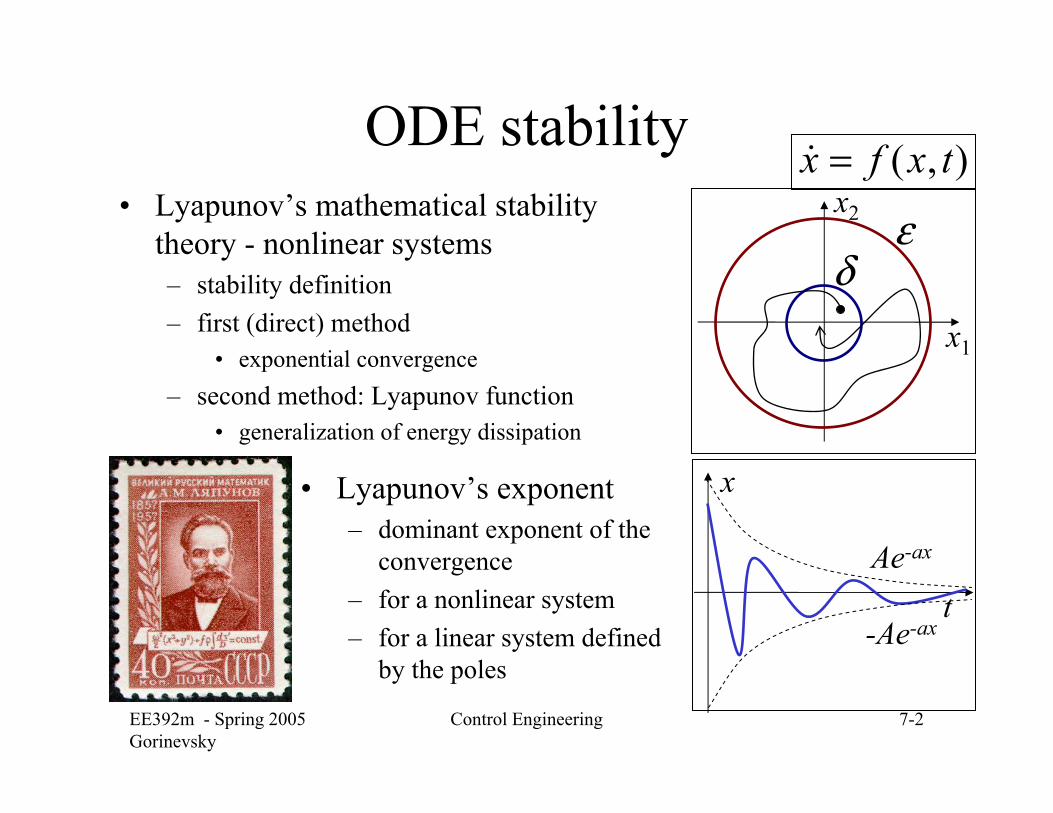
ODE stability• Lyapunov’s mathematical stability

theory - nonlinear systems– stability definition– first (direct) method

• exponential convergence– second method: Lyapunov function

• generalization of energy dissipation

x1

x2

• Lyapunov’s exponent– dominant exponent of the

convergence– for a nonlinear system– for a linear system defined

by the poles

t

x

Ae-ax

-Ae-ax

),( txfx =&

εδ



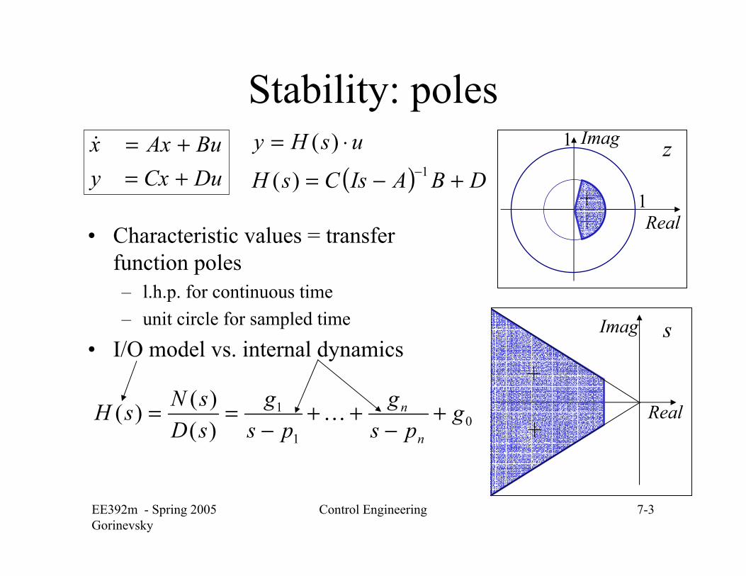
Stability: poles

• Characteristic values = transfer function poles– l.h.p. for continuous time– unit circle for sampled time

• I/O model vs. internal dynamics

Real

Imag s

Real

Imag1

1

z( ) DBAIsCsH

usHy

+−=

⋅=−1)(

)(DuCxyBuAxx

+=+=&

01

1

)()()( g

psg

psg

sDsNsH

n

n +−

++−

== K



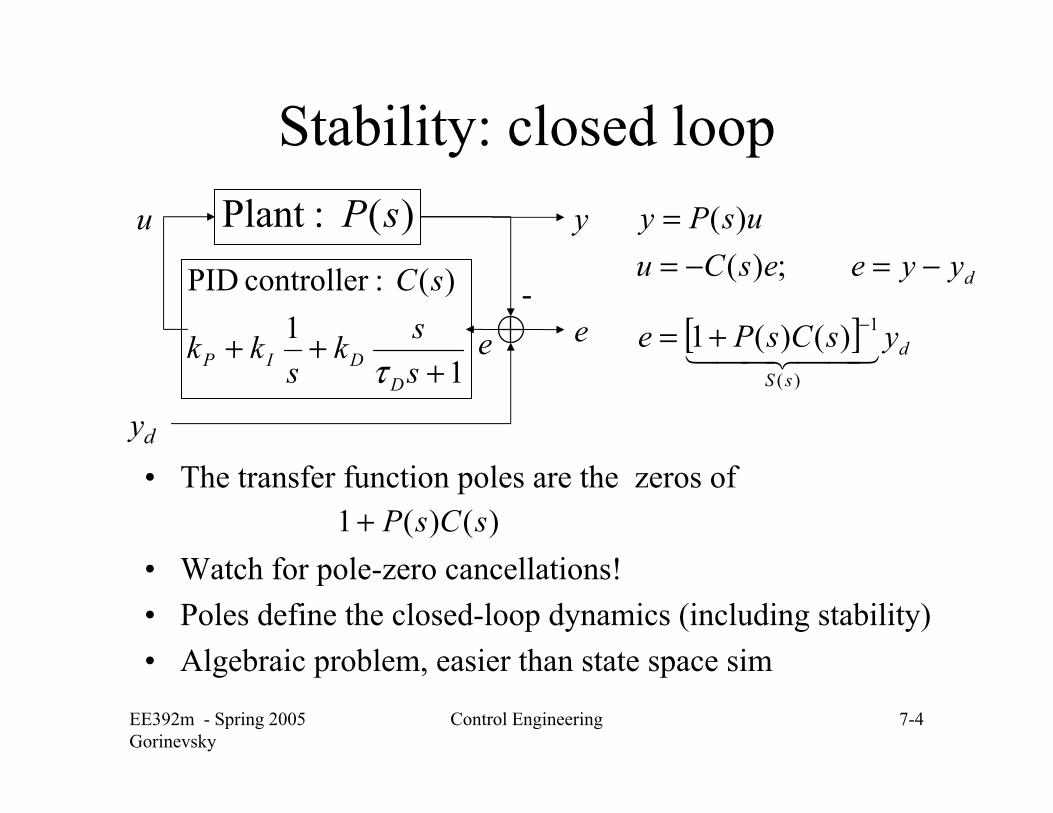
Stability: closed loop

• The transfer function poles are the zeros of

• Watch for pole-zero cancellations!• Poles define the closed-loop dynamics (including stability) • Algebraic problem, easier than state space sim

11

)( :controller PID

+++

ssk

skk

sC

DDIP τ

)( :Plant sP

-e e

y

yd

u

dyyeesCuusPy

−=−==

;)()(

[ ] d

sS

ysCsPe 44 344 21)(

1)()(1 −+=

)()(1 sCsP+



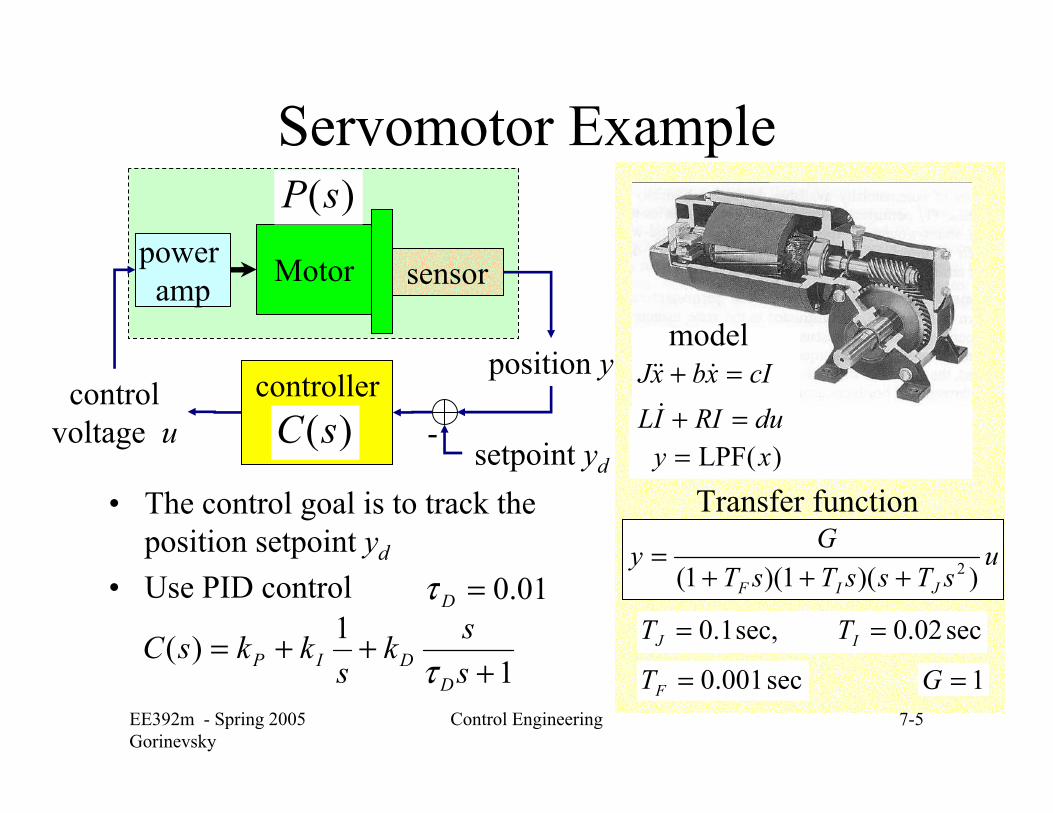
Servomotor Example

• The control goal is to track the position setpoint yd

• Use PID control

model

usTssTsT

GyJIF ))(1)(1( 2+++

=

Transfer function

sec02.0sec,1.0 == IJ TT

Motorpower amp sensor

position ycontrol

voltage usetpoint yd

controller-

)(LPF xy =duRIILcIxbxJ

=+=+

&

&&&

1=G

)(sP

)(sC

11)(

+++=

ssk

skksC

DDIP τ

01.0=Dτ

sec 001.0=FT



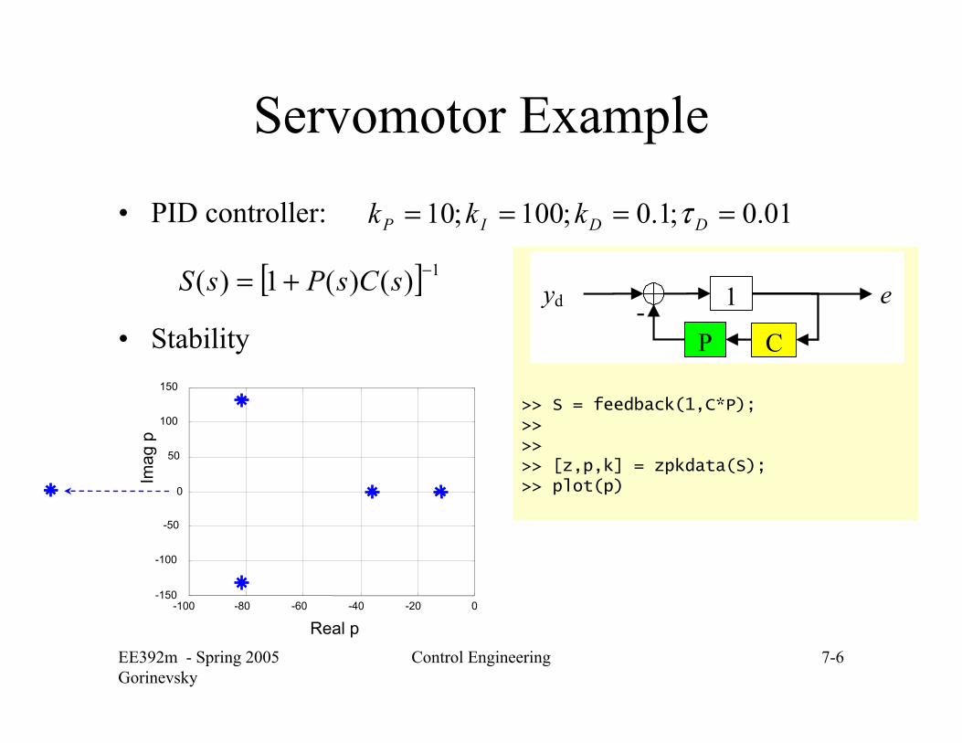
Servomotor Example

• PID controller:

• Stability

01.0;1.0;100;10 ==== DDIP kkk τ

[ ] 1)()(1)( −+= sCsPsS

>> S = feedback(1,C*P);>>>>>> [z,p,k] = zpkdata(S);>> plot(p)

e- 1yd

CP

-100 -80 -60 -40 -20 0-150

-100

-50

0

50

100

150

Real p

Imag

p



Stability

• … almost, except the critical stability• For nonlinear systems

– linearize around the equilibrium– might have to look at the stability theory -

Lyapunov• Orbital stability:

– trajectory converges to the desired– the state does not - the timing is off

• spacecraft• FMS, 3-D trajectories without aircraft

arrival time

For linear system poles describe stability



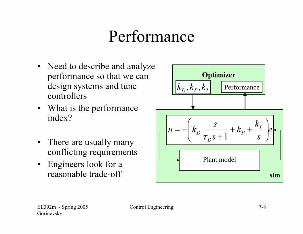
Performance• Need to describe and analyze

performance so that we can design systems and tune controllers

• What is the performance index?

• There are usually many conflicting requirements

• Engineers look for a reasonable trade-off sim

eskk

ssku I

PD

D ⎟⎟⎠

⎞⎜⎜⎝

⎛++

+−=

1τ

Plant model

Optimizer

IPD kkk ,, Performance



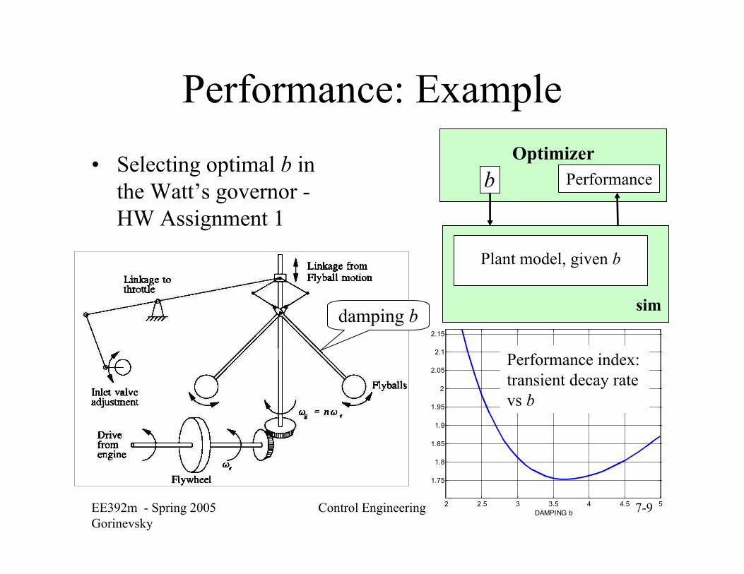
Performance: Example

• Selecting optimal b in the Watt’s governor -HW Assignment 1

sim

Plant model, given b

Optimizerb Performance

2 2.5 3 3.5 4 4.5 5

1.75

1.8

1.85

1.9

1.95

2

2.05

2.1

2.15

DAMPING b

Performance index:transient decay rate vs b

damping b



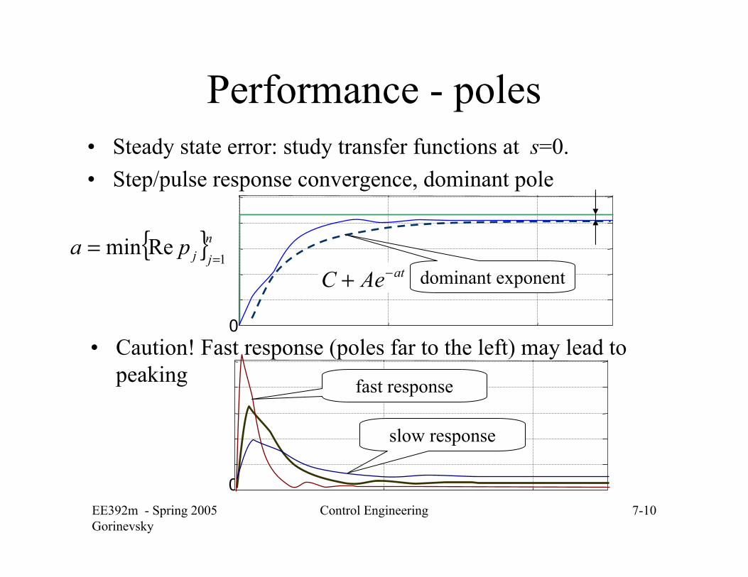
Performance - poles• Steady state error: study transfer functions at s=0.• Step/pulse response convergence, dominant pole

• Caution! Fast response (poles far to the left) may lead to peaking

0

slow response

fast response

{ }njjpa

1Remin

==

0

atAeC −+ dominant exponent



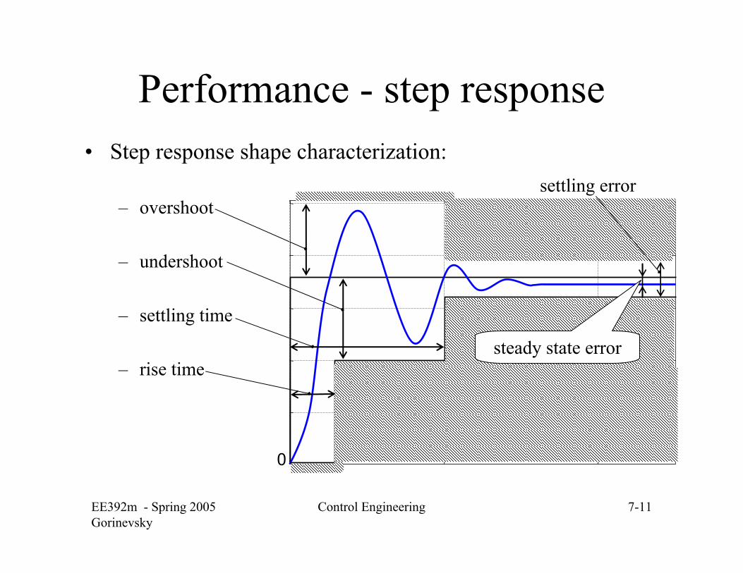
Performance - step response• Step response shape characterization:

– overshoot

– undershoot

– settling time

– rise time

0

steady state error

settling error



Performance - quadratic index

• Quadratic performance – response, in frequency domain

0

{ω

ωω

πωωω

π

ωωπ

diSdiyiS

diedttytyJ

d

td

∫∫

∫∫

=

==−=∞

∞

∞

=

STEP

222

2

0

2

1)(21)(~)(

21

)(~21)()(

• For yd(t) a zero mean random process with spectral power Q (iω)

• For Q (iω) =1, this is just Parceval’s theorem

ωωωπ

diQiSdttytyEJt

d )()(21)()( 2

0

2

∫∫ =⎟⎟⎠

⎞⎜⎜⎝

⎛−=

∞

=

[ ] 1)()(1)( −+= sCsPsS



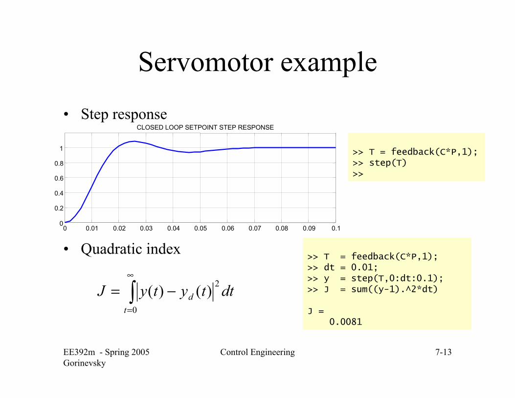
Servomotor example

• Step response

• Quadratic index

>> T = feedback(C*P,1); >> step(T)>>

>> T = feedback(C*P,1); >> dt = 0.01;>> y = step(T,0:dt:0.1); >> J = sum((y-1).^2*dt)

J =0.0081

∫∞

=

−=0

2)()(t

d dttytyJ

0 0.01 0.02 0.03 0.04 0.05 0.06 0.07 0.08 0.09 0.10

0.2

0.4

0.6

0.8

1

CLOSED LOOP SETPOINT STEP RESPONSE



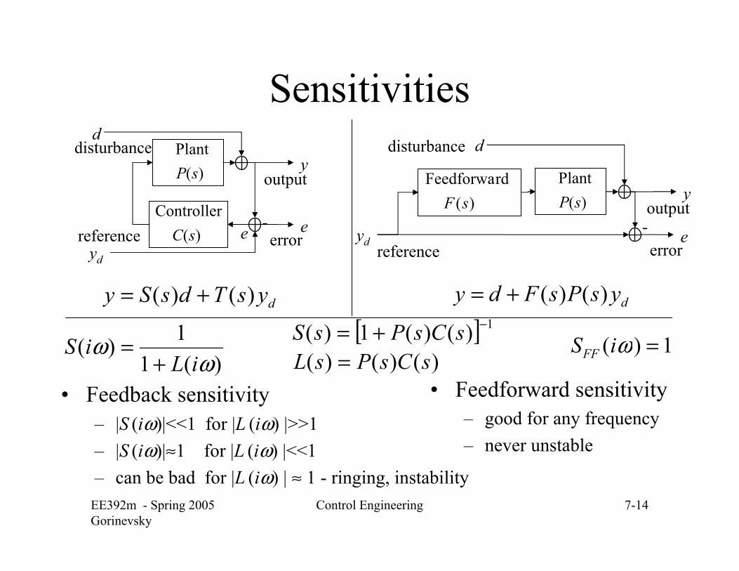
Sensitivities

• Feedback sensitivity – |S (iω)|<<1 for |L (iω) |>>1– |S (iω)|≈1 for |L (iω) |<<1– can be bad for |L (iω) | ≈ 1 - ringing, instability

dysTdsSy )()( +=

)(11)(

ωω

iLiS

+=

)( rd Feedforwa

sF )( Plant

sP- e

y

yd

ddisturbance

reference

output

error)(

Controller sC

)( Plant

sP

-e e

y

yd

ddisturbance

reference

output

error

dysPsFdy )()(+=

• Feedforward sensitivity– good for any frequency– never unstable

1)( =ωiSFF[ ] 1)()(1)( −+= sCsPsS

)()()( sCsPsL =



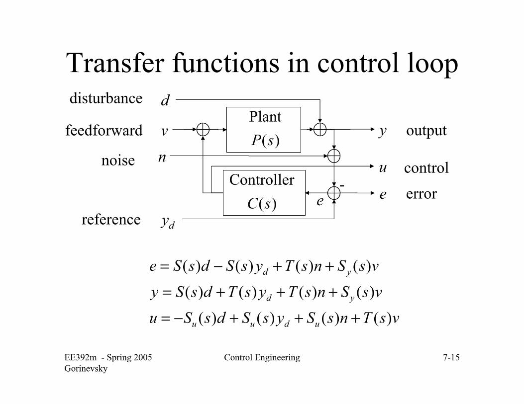
Transfer functions in control loop

vsTnsSysSdsSuvsSnsTysTdsSyvsSnsTysSdsSe

uduu

yd

yd

)()()()()()()()()()()()(

+++−=

+++=

++−=

)( Controller

sC

)( Plant

sP

-e e

y

yd

v

u

ddisturbance

feedforward

reference

output

controlerror

nnoise



Transfer functions in control loop

Sensitivity

Complementary sensitivity

Noise sensitivity

Load sensitivity

[ ][ ][ ][ ] )()()(1)(

)()()(1)(

)()()()(1)(

)()(1)(

1

1

1

1

sPsCsPsS

sCsCsPsS

sCsPsCsPsT

sCsPsS

y

u−

−

−

−

+=

+=

+=

+=

esCudvusPy

nyye d

)())((

−=++=

+−=


uduu

yd

yd

)()()()()()()()()()()()(

+++−=

+++=

++−=

S(s) + T(s) = 1



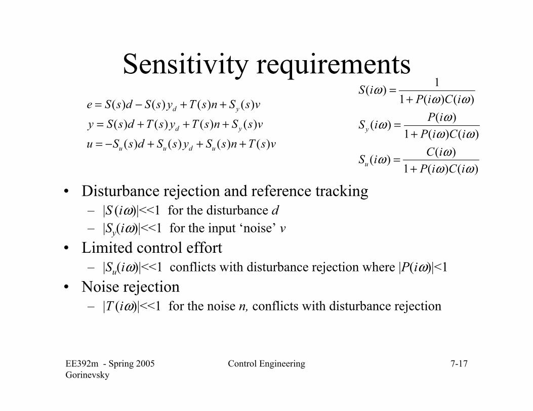
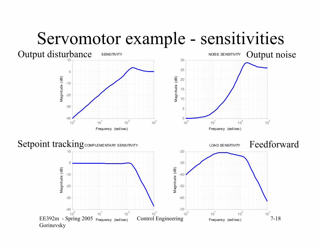
Sensitivity requirements

• Disturbance rejection and reference tracking– |S (iω)|<<1 for the disturbance d– |Sy(iω)|<<1 for the input ‘noise’ v

• Limited control effort– |Su(iω)|<<1 conflicts with disturbance rejection where |P(iω)|<1

• Noise rejection – |T (iω)|<<1 for the noise n, conflicts with disturbance rejection

)()(1)()(

)()(1)()(

)()(11)(

ωωωω

ωωωω

ωωω

iCiPiCiS

iCiPiPiS

iCiPiS

u

y

+=

+=

+=


uduu

yd

yd

)()()()()()()()()()()()(

+++−=

+++=

++−=



Servomotor example - sensitivities

Setpoint tracking

Output disturbance Output noise

Feedforward

100 101 102 103-40

-30

-20

-10

0

10M

agni

tude

(dB

)

SENSITIVITY

Frequency (rad/sec)

100

101

102

103

-40

-30

-20

-10

0

10

Mag

nitu

de (

dB)

COMPLEMENTARY SENSITIVITY

Frequency (rad/sec)

100 101 102 1030

5

10

15

20

25

30

Mag

nitu

de (

dB)

NOISE SENSITIVITY

Frequency (rad/sec)

100

101

102

103

-70

-60

-50

-40

-30

-20

Mag

nitu

de (

dB)

LOAD SENSITIVITY

Frequency (rad/sec)



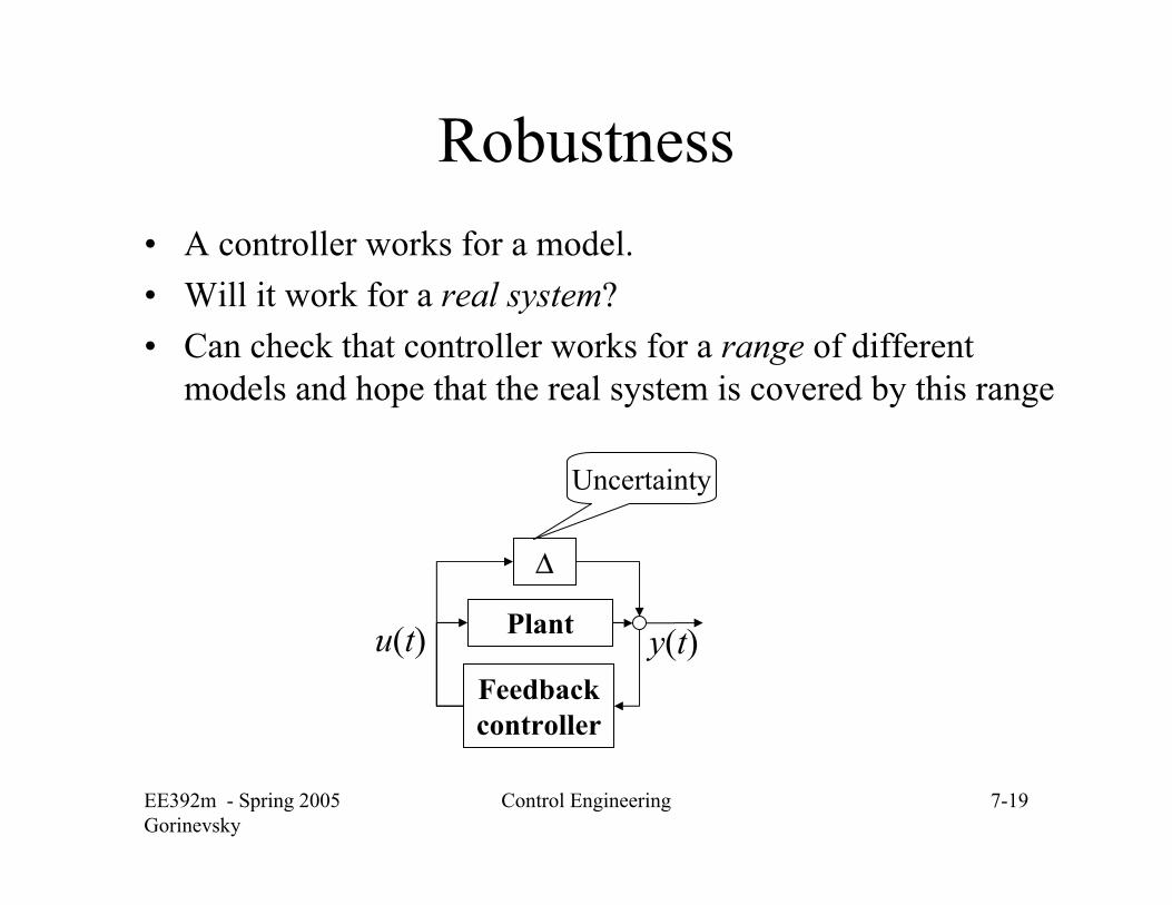
Robustness• A controller works for a model. • Will it work for a real system?• Can check that controller works for a range of different

models and hope that the real system is covered by this range

Plant

Feedback controller

y(t)u(t)

∆

Uncertainty



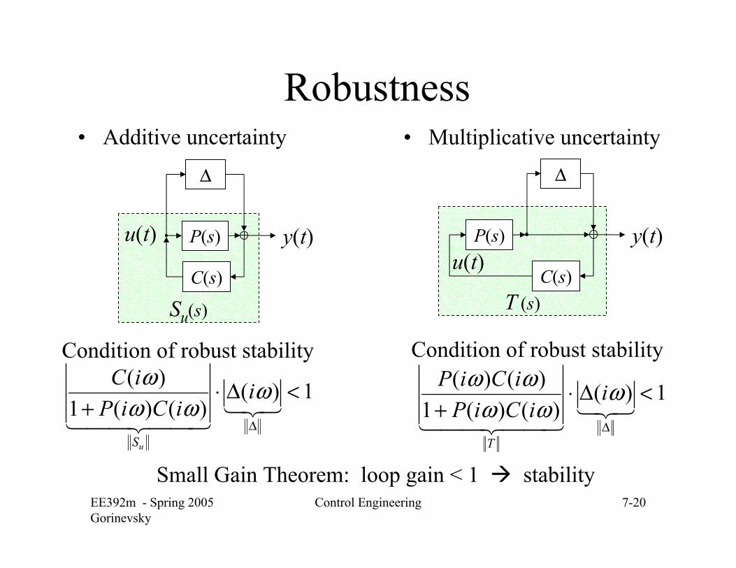
Robustness• Additive uncertainty

T (s)

P(s)

C(s)

y(t)u(t)

∆

1)()()(1

)()( <∆⋅+

∆321

44 344 21

ωωω

ωω iiCiP

iCiP

T

Condition of robust stability

Su(s)

P(s)

C(s)

y(t)u(t)

∆

1)()()(1

)( <∆⋅+

∆321

44 344 21

ωωω

ω iiCiP

iC

uS

Condition of robust stability

• Multiplicative uncertainty

Small Gain Theorem: loop gain < 1 stability



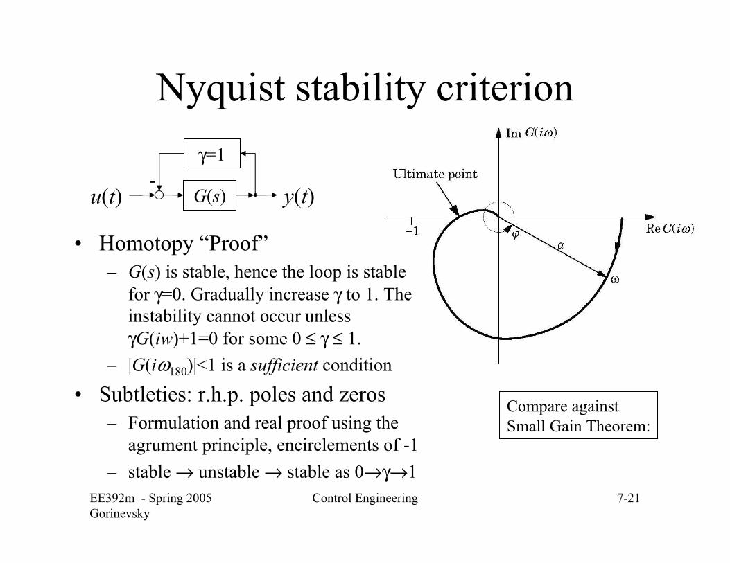
Nyquist stability criterion

• Homotopy “Proof” – G(s) is stable, hence the loop is stable

for γ=0. Gradually increase γ to 1. The instability cannot occur unless γG(iw)+1=0 for some 0 ≤ γ ≤ 1.

– |G(iω180)|<1 is a sufficient condition

• Subtleties: r.h.p. poles and zeros– Formulation and real proof using the

agrument principle, encirclements of -1– stable → unstable → stable as 0→γ→1

u(t) G(s) y(t)

γ=1

Compare against Small Gain Theorem:

-



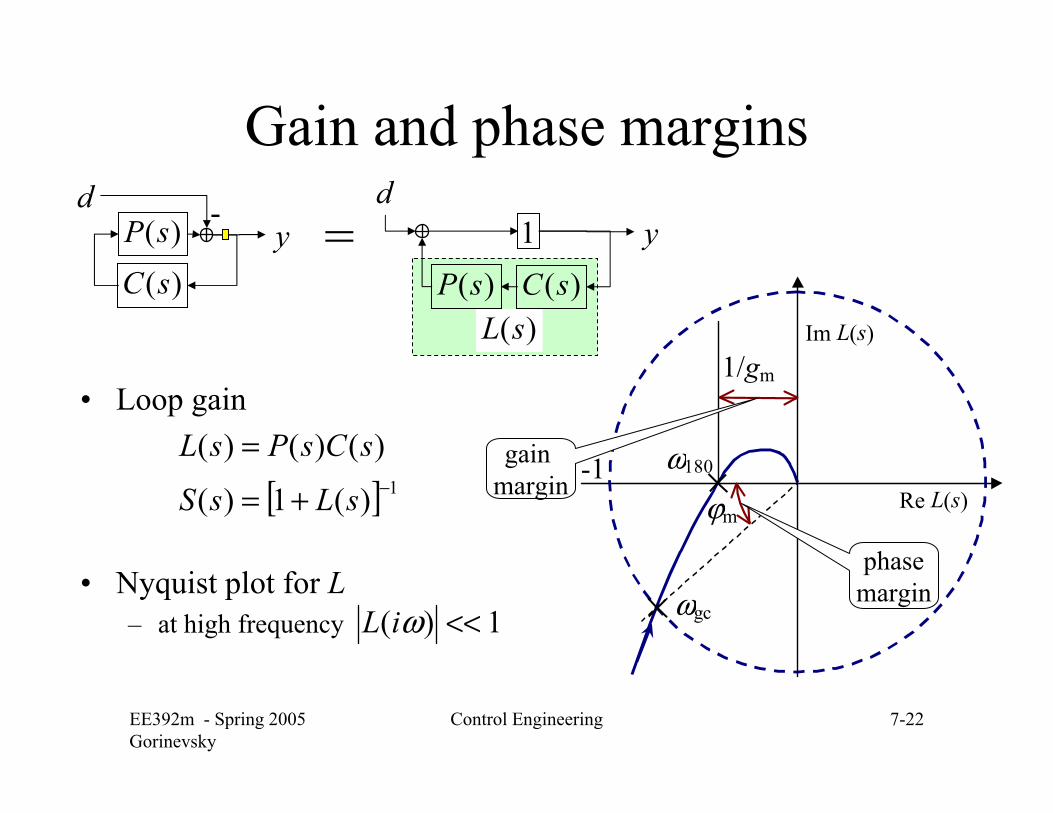
Gain and phase margins

• Loop gain

• Nyquist plot for L– at high frequency

Im L(s)

Re L(s)

1/gm

ω180

ωgc

ϕm

-1

=

[ ] 1)(1)(

)()()(−+=

=

sLsS

sCsPsL gain margin

phasemargin

1)( <<ωiL

)(sC)(sP -

yd

)(sP )(sCy

d1

)(sL



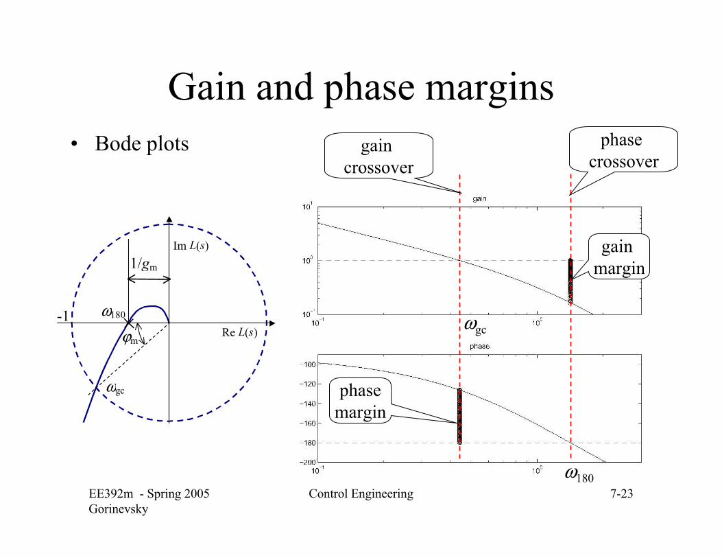
Gain and phase margins• Bode plots

Im L(s)

Re L(s)

1/gm

ω180

ωgc

ϕm

-1

ω180

ωgc

gain crossover

phase crossover

gain margin

phasemargin



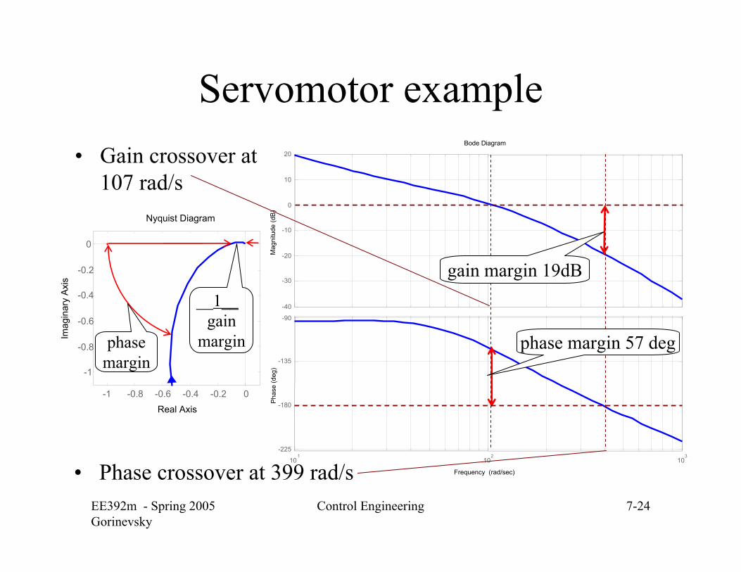
Servomotor example• Gain crossover at

107 rad/s

-40

-30

-20

-10

0

10

20

Mag

nitu

de (d

B)

101

102

103

-225

-180

-135

-90

Bode Diagram

Frequency (rad/sec)

Pha

se (d

eg)

gain margin 19dB

phase margin 57 deg

Nyquist Diagram

Real Axis

Imag

inar

y Ax

is

-1 -0.8 -0.6 -0.4 -0.2 0

-1

-0.8

-0.6

-0.4

-0.2

0

phasemargin

__1__ gain

margin

• Phase crossover at 399 rad/s

Date post:	07-Jul-2020
Category:	Documents
Upload:	others
View:	13 times
Download:	0 times

Lecture7 SISO Analysis€¦ · EE392m - Spring 2005 Gorinevsky Control Engineering 7-1 Lecture 7 -...

Documents