207
UNIVERSITY OF WATERLOO Department of Economics LECTURE NOTES For the course Numerical Methods for Economists Author Pierre Chauss ´ e
| Date post: | 03-Jan-2016 |
| Category: |
Documents |
| Upload: | rodolfohcc7219 |
| View: | 76 times |
| Download: | 2 times |
UNIVERSITY OF WATERLOO
Department of Economics
L E C T U R E N O T E S
For the course
Numerical Methods for Economists
Author
Pierre Chausse

Contents
1 Introduction to R 5
1.1 Getting help . . . . . . . . . . . . . . . . . . . . . . . . . . . . . . . . . . 5
1.2 The basic concepts . . . . . . . . . . . . . . . . . . . . . . . . . . . . . . 7
1.2.1 Understanding the structure . . . . . . . . . . . . . . . . . . . . . 7
1.3 Organizing our programs . . . . . . . . . . . . . . . . . . . . . . . . . . . 23
1.3.1 Classes and methods for second order polynomials . . . . . . . . 30
1.4 Programming efficiently . . . . . . . . . . . . . . . . . . . . . . . . . . . 39
1.4.1 Loops versus matrix operations . . . . . . . . . . . . . . . . . . . 39
1.4.2 Parallel programming . . . . . . . . . . . . . . . . . . . . . . . . 45
2 Floating points arithmetic 49
2.1 What is a floating-point number . . . . . . . . . . . . . . . . . . . . . . 49
2.2 Rounding errors . . . . . . . . . . . . . . . . . . . . . . . . . . . . . . . . 54
3 Linear Equations and Iterative Methods 59
3.1 Linear algebra . . . . . . . . . . . . . . . . . . . . . . . . . . . . . . . . . 59
3.2 Iterative method . . . . . . . . . . . . . . . . . . . . . . . . . . . . . . . 66
3.2.1 Stopping rules . . . . . . . . . . . . . . . . . . . . . . . . . . . . 66
3.2.2 Fixed-Point Iteration . . . . . . . . . . . . . . . . . . . . . . . . . 70
3.2.3 Gauss-Jacobi and Gauss-Seidel . . . . . . . . . . . . . . . . . . . 71
3.2.4 Acceleration and Stabilization Methods . . . . . . . . . . . . . . 78
4 Optimization 85
4.1 One-dimensional problems . . . . . . . . . . . . . . . . . . . . . . . . . . 85
4.2 Multidimensional Optimization . . . . . . . . . . . . . . . . . . . . . . . 94
4.2.1 A monopoly problem . . . . . . . . . . . . . . . . . . . . . . . . . 94
4.2.2 Newton’s Method . . . . . . . . . . . . . . . . . . . . . . . . . . . 97
4.2.3 Direction Set Methods . . . . . . . . . . . . . . . . . . . . . . . . 101
4.2.4 Finite Differences . . . . . . . . . . . . . . . . . . . . . . . . . . . 108
4.3 Constrained optimization . . . . . . . . . . . . . . . . . . . . . . . . . . 109
4.4 Applications . . . . . . . . . . . . . . . . . . . . . . . . . . . . . . . . . . 112
4.4.1 Principal-Agent Problem . . . . . . . . . . . . . . . . . . . . . . 112
4.4.2 Efficient Outcomes with Adverse Selection . . . . . . . . . . . . . 112
4.4.3 Computing Nash Equilibrium. . . . . . . . . . . . . . . . . . . . 113
4.4.4 Portfolio Problem . . . . . . . . . . . . . . . . . . . . . . . . . . 114
4.4.5 Dynamic Optimization . . . . . . . . . . . . . . . . . . . . . . . . 115
2 Contents
5 Nonlinear Equations 117
5.1 One-dimensional problems . . . . . . . . . . . . . . . . . . . . . . . . . . 117
5.1.1 The Bisection Method . . . . . . . . . . . . . . . . . . . . . . . . 120
5.1.2 Newton’s Method . . . . . . . . . . . . . . . . . . . . . . . . . . . 125
5.2 Multivariate Nonlinear Equations . . . . . . . . . . . . . . . . . . . . . . 128
5.2.1 Newton’s Method . . . . . . . . . . . . . . . . . . . . . . . . . . . 129
5.2.2 Gauss Methods . . . . . . . . . . . . . . . . . . . . . . . . . . . . 130
5.2.3 Broyden’s Method . . . . . . . . . . . . . . . . . . . . . . . . . . 132
5.2.4 The nleqslv package . . . . . . . . . . . . . . . . . . . . . . . . . 133
5.2.5 Example . . . . . . . . . . . . . . . . . . . . . . . . . . . . . . . . 134
6 Numerical Calculus 137
6.1 Numerical Integration . . . . . . . . . . . . . . . . . . . . . . . . . . . . 137
6.1.1 Newton-Cotes . . . . . . . . . . . . . . . . . . . . . . . . . . . . . 138
6.1.2 Gauss Methods . . . . . . . . . . . . . . . . . . . . . . . . . . . . 142
6.1.3 Numerical integration with R . . . . . . . . . . . . . . . . . . . . 146
6.1.4 Numerical derivatives with R . . . . . . . . . . . . . . . . . . . . 147
7 Monte Carlo Simulation 149
7.1 Introduction . . . . . . . . . . . . . . . . . . . . . . . . . . . . . . . . . . 149
7.2 Econometrics . . . . . . . . . . . . . . . . . . . . . . . . . . . . . . . . . 153
7.3 Integration . . . . . . . . . . . . . . . . . . . . . . . . . . . . . . . . . . 154
7.4 To be completed latter . . . . . . . . . . . . . . . . . . . . . . . . . . . . 155
8 Differential Equations 157
8.1 Introduction . . . . . . . . . . . . . . . . . . . . . . . . . . . . . . . . . . 157
8.2 Finite Difference Methods for initial value problems . . . . . . . . . . . 159
8.2.1 Euler’s Method . . . . . . . . . . . . . . . . . . . . . . . . . . . . 160
8.2.2 Implicit Euler’s Method . . . . . . . . . . . . . . . . . . . . . . . 161
8.2.3 Trapezoid Rule . . . . . . . . . . . . . . . . . . . . . . . . . . . . 162
8.2.4 Runge-Kutta Method . . . . . . . . . . . . . . . . . . . . . . . . 163
8.2.5 Example: Signaling Equilibrium . . . . . . . . . . . . . . . . . . 165
8.3 Boundary values and the Shooting Method . . . . . . . . . . . . . . . . 167
8.3.1 Infinite Horizon Models . . . . . . . . . . . . . . . . . . . . . . . 171
8.4 Projection Methods (incomplete) . . . . . . . . . . . . . . . . . . . . . . 178
8.5 Partial Differential Equation: The Heat Equation . . . . . . . . . . . . . 184
8.5.1 Black and Scholes and the Heat Equation . . . . . . . . . . . . . 189
8.6 R packages for differential equations . . . . . . . . . . . . . . . . . . . . 190
A Solution to some Problems 193
A.1 Chapter 1 . . . . . . . . . . . . . . . . . . . . . . . . . . . . . . . . . . . 193

Contents 3
Bibliography 205

Chapter 1
Introduction to R
Contents
1.1 Getting help . . . . . . . . . . . . . . . . . . . . . . . . . . . . . . 5
1.2 The basic concepts . . . . . . . . . . . . . . . . . . . . . . . . . . . 7
1.2.1 Understanding the structure . . . . . . . . . . . . . . . . . . . . . . 7
1.3 Organizing our programs . . . . . . . . . . . . . . . . . . . . . . . 23
1.3.1 Classes and methods for second order polynomials . . . . . . . . . 30
1.4 Programming efficiently . . . . . . . . . . . . . . . . . . . . . . . 39
1.4.1 Loops versus matrix operations . . . . . . . . . . . . . . . . . . . . 39
1.4.2 Parallel programming . . . . . . . . . . . . . . . . . . . . . . . . . 45
1.1 Getting help
You can find R on the official web site http://www.r-project.org/. It is available for
Windows, Mac and Linux. As for any open source software, there are several manuals
on R that can be downloaded from the internet for free. On the web site (http://cran.r-
project.org/manuals.html), you will find detailed manuals for both users and develop-
ers. I recommend going through sections 1 to 9 of ”An Introduction to R”, which
will give you what you need to get started. The manual ”R Data Import/Export” is
a complete reference on how to deal with data from different sources (Stata, Matlab,
Excel, etc.). There are also manuals specialized in econometrics. I suggest download-
ing http://cran.r-project.org/doc/contrib/Farnsworth-EconometricsInR.pdf. Finally,
there are several books published by Springer for any area of econometrics which are
not too expensive.
There are also tools integrated in R which are helpful when we are looking for a
particular function or when we want to know how to use it. Suppose we want to know
how to generate random numbers, but we don’t know the name of the function. We
can search using key words :
> help.search("Normal Distribution")
6 Chapter 1. Introduction to R
which gives a list of functions for which ”Normal Distribution” is in the description. For
example, one of the results is ”stats::Normal The Normal Distribution”, which means
that the function ”Normal” can be found in the package ”stats”. The latter is included
in R and therefore do not need to be added. However, the result ”mnormt::dmnorm
Multivariate normal distribution” refers to the function dmnorm() which belongs to the
package ”mvtnorm” of [Genz et al. 2011]. This is one of the many packages that can
be found on CRAN (see the list here: http://probability.ca/cran/web/packages/) and
which can be installed using:
> install.packages("mvtnorm")
Once we have found the function we are looking for, we use the help() function in order
to learn the syntax. For example, if we are interested by the above result ”Normal”, we
type:
> help("Normal")
Notice that R is case sensitive. If you type help(”normal”), you will get an error message.
There are four functions associated with the term ”Normal”. The help file starts with
the syntax of these functions:
dnorm(x, mean = 0, sd = 1, log = FALSE)
pnorm(q, mean = 0, sd = 1, lower.tail = TRUE, log.p = FALSE)
qnorm(p, mean = 0, sd = 1, lower.tail = TRUE, log.p = FALSE)
rnorm(n, mean = 0, sd = 1)
Some arguments such as ”mean” have default values and others such as ”x” or ”q”
require a value. Here is some examples:
� The density of a N(0,1) evaluated at 0.5:
> dnorm(0.5)
[1] 0.3520653
� The logarithm of the density of a N(0,1) evaluated at 0.5:
> dnorm(0.5,log=TRUE)
[1] -1.043939
� The density of a N(5,10) evaluated at 2:
> dnorm(2,mean=5,sd=sqrt(10))
1.2. The basic concepts 7
[1] 0.08044102
� 5 pseudo random numbers from a N(0,1) using the seed 123:
> set.seed(123)
> rnorm(5)
[1] -0.56047565 -0.23017749 1.55870831 0.07050839 0.12928774
There are no secret tricks to learn a computer language. You need to sit down and
work hard. The best way is to think about a numerical project and try to do it. And
remember that if you have a problem, someone must have gone through the same.
The answer is probably somewhere in a newsgroup. Internet search engines such as
Google are therefore endless sources of information. You can even participate and ask
a question. But remember that the persons who answer are usually very friendly and
work for free. Therefore, show them that you have made an effort before asking a
question otherwise you could get the answer rtfm (read the f... manual).
Exercise 1.1. Using the help() or help.search(), try to find a function that: (i) solves
the system Ax = b, (ii) estimates a linear model by OLS, (iii) gives you the number of
characters in a string such as ”hello” and (iv) computes the mean of each column of a
matrix.
1.2 The basic concepts
1.2.1 Understanding the structure
R is an object-oriented language. The only difference between an object-oriented lan-
guage and one which is not object-oriented is the organization of functions and elements.
For example, the following
> x <- 1
> print(x)
[1] 1
means that the new object ”x” receives all the attributes of the right-hand side. In that
case, the operators ”=” and ”<-” are identical. However, it is often suggested to always
use the latter when defining an object. The former is used when we set the options in
a function:
> y <- matrix(1,nrow=1, ncol = 1)
> print(y)
8 Chapter 1. Introduction to R
[,1]
[1,] 1
To see the difference, the two-line code above can be written in one single line as:
> print(y <- matrix(1,nrow=1, ncol = 1))
[,1]
[1,] 1
It defines the object ”y” and then print it. In that case, the operator ”=” cannot be
used; try
> print(y = matrix(1,nrow=1, ncol = 1))
An object is defined by its attributes and classes. Objects of some classes don’t have any
attributes and some have many. For example, x and y, defined above, look identical.
But they are different objects. We can obtain the classes associated with an object by
using the function ”is()”:
> is(x)
[1] "numeric" "vector"
> is(y)
[1] "matrix" "array" "structure" "vector"
and the attributes with ”attributes()”:
> attributes(x)
NULL
> attributes(y)
$dim
[1] 1 1
The difference between these two objects is that x does not have the attribute ”dim”
which gives the dimension of an array. Therefore we could make x identical to y simply
by adding the attribute ”dim” to it as follows:
> attributes(x) <- list(dim=c(1,1))
> is(x)
1.2. The basic concepts 9
[1] "matrix" "array" "structure" "vector"
However, this is not the most efficient way to transform the object x. We would
obtain the same result with the command ”x <- as.matrix(x)”. It is very important to
understand the difference between vectors with and without the attribute ”dim”. The
usual matrix operations can be performed only if the objects have the attribute ”dim”.
If they don’t, the operations can produce unexpected results. To see that, let A be a
2× 2 matrix and x be a simple vector (without ”dim”) containing two elements.
> A <- matrix(c(1,2,3,4),2,2)
> A
[,1] [,2]
[1,] 1 3
[2,] 2 4
> x <- c(1,2)
> x
[1] 1 2
Additions of two matrices are allowed only if the dimensions coincide. Because x does
not have any dimension, the operation A + x is allowed. But we have to be careful
with how R treats such operations. In fact, a matrix of the same dimension as A is
constructed by repeating the vector x until the total number of elements is equal to
the number of elements of A. Therefore, the number of elements of A should be a
multiple of the number of elements of x. A warning message is printed otherwise (try
to experiment as much cases as possible to make sure you understand). The result is:
> A+x
[,1] [,2]
[1,] 2 4
[2,] 4 6
However, if x is a 2×1 matrix, R returns an error message (Here I use the function try()
which returns the result if the operation is allowed and an error message otherwise):
> x <- as.matrix(x)
> try(x+A)[1]
[1] "Error in x + A : non-conformable arrays\n"
10 Chapter 1. Introduction to R
This way of treating operations may seem confusing at first, but it happens to be very
useful in some cases. Suppose you have a T×N matrix R of asset returns. Each column
represents a different time series of returns. You also have a time series of returns on
the three-month US treasury bill (Rf ) that you want to use as proxy for the risk-free
rate. To compute a time series of excess returns of each asset (Zit = Rit − Rft), you
can simply define the vector of risk-free rates as a simple vector and do
> Z<- R-Rf
There are also different kinds of vector. We can create a vector of messages:
> W <- c("hello!", "Bonjour!", "Ohayogozaimasu!")
> is(W)
[1] "character" "vector" "data.frameRowLabels"
[4] "SuperClassMethod"
It is a vector, which means that it is a collection of elements, but we don’t see the
class ”numeric”. Therefore, mathematical operations are not allowed on that kind of
objects. In C++, which is probably the most popular object-oriented language for
software developers, you can redefine the operator ”+” for vectors of characters. It
would, for example, construct a new vector by combining the characters of each vector.
The operator ”+” would react differently whether the vector is numeric or not. There
is no point of having such operators in R, but it shows how it works. Many functions
are built in such a way that they react differently depending on the type of objects.
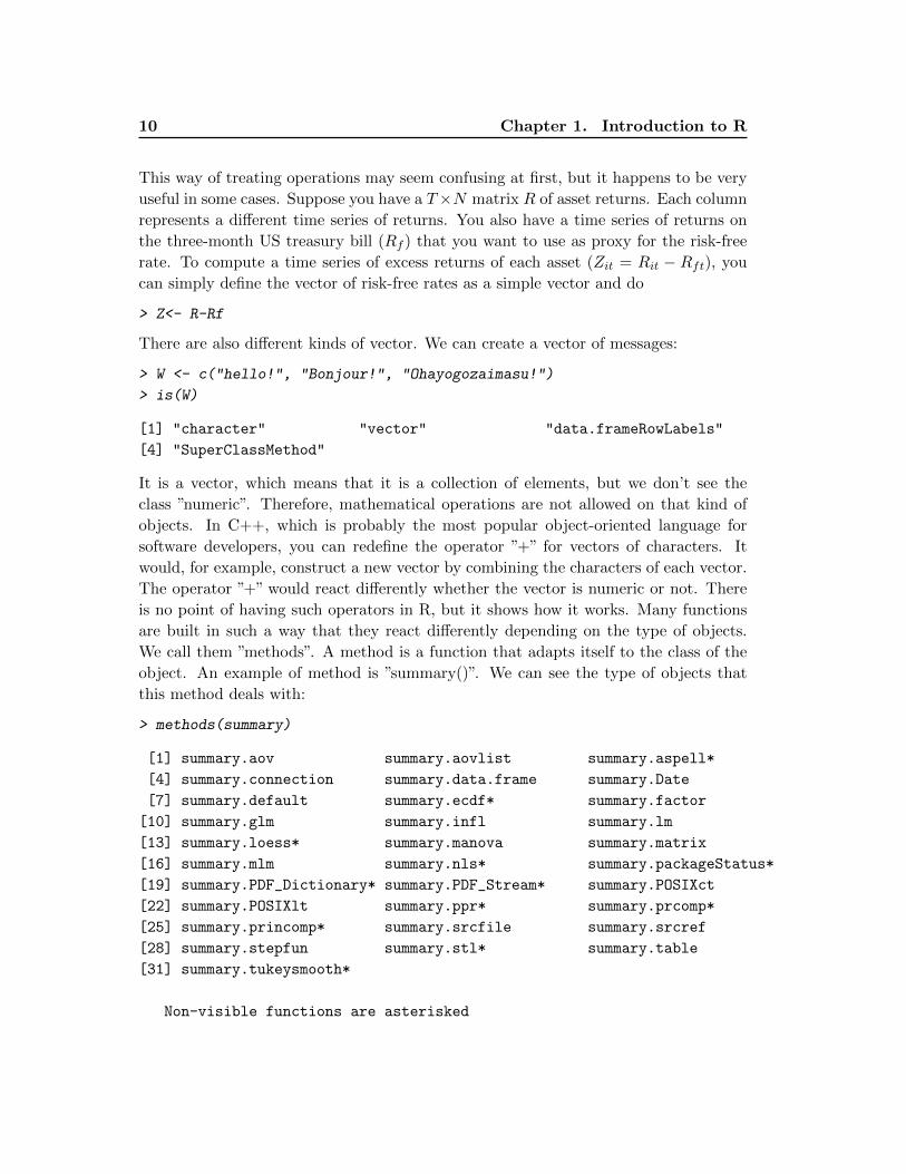
We call them ”methods”. A method is a function that adapts itself to the class of the
object. An example of method is ”summary()”. We can see the type of objects that
this method deals with:
> methods(summary)
[1] summary.aov summary.aovlist summary.aspell*
[4] summary.connection summary.data.frame summary.Date
[7] summary.default summary.ecdf* summary.factor
[10] summary.glm summary.infl summary.lm
[13] summary.loess* summary.manova summary.matrix
[16] summary.mlm summary.nls* summary.packageStatus*
[19] summary.PDF_Dictionary* summary.PDF_Stream* summary.POSIXct
[22] summary.POSIXlt summary.ppr* summary.prcomp*
[25] summary.princomp* summary.srcfile summary.srcref
[28] summary.stepfun summary.stl* summary.table
[31] summary.tukeysmooth*
Non-visible functions are asterisked
1.2. The basic concepts 11
The class of the object appears after the dot. So, summary() will treat objects of class
”matrix ” differently from objects of class, say, ”data.frame”. Other classes not listed
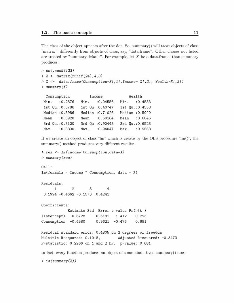
are treated by ”summary.default”. For example, let X be a data.frame, than summary
produces:
> set.seed(123)
> X <- matrix(runif(24),4,3)
> X <- data.frame(Consumption=X[,1],Income= X[,2], Wealth=X[,3])
> summary(X)
Consumption Income Wealth
Min. :0.2876 Min. :0.04556 Min. :0.4533
1st Qu.:0.3786 1st Qu.:0.40747 1st Qu.:0.4558
Median :0.5986 Median :0.71026 Median :0.5040
Mean :0.5920 Mean :0.60164 Mean :0.6046
3rd Qu.:0.8120 3rd Qu.:0.90443 3rd Qu.:0.6528
Max. :0.8830 Max. :0.94047 Max. :0.9568
If we create an object of class ”lm” which is create by the OLS procedure ”lm()”, the
summary() method produces very different results:
> res <- lm(Income~Consumption,data=X)
> summary(res)
Call:
lm(formula = Income ~ Consumption, data = X)
Residuals:
1 2 3 4
0.1994 -0.4662 -0.1573 0.4241
Coefficients:
Estimate Std. Error t value Pr(>|t|)
(Intercept) 0.8728 0.6181 1.412 0.293
Consumption -0.4580 0.9621 -0.476 0.681
Residual standard error: 0.4805 on 2 degrees of freedom
Multiple R-squared: 0.1018, Adjusted R-squared: -0.3473
F-statistic: 0.2266 on 1 and 2 DF, p-value: 0.681
In fact, every function produces an object of some kind. Even summary() does:
> is(summary(X))
12 Chapter 1. Introduction to R
[1] "table" "oldClass"
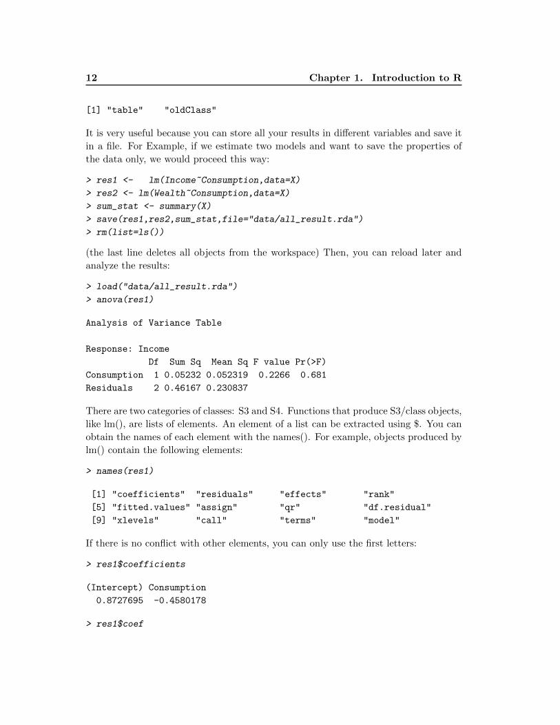
It is very useful because you can store all your results in different variables and save it
in a file. For Example, if we estimate two models and want to save the properties of
the data only, we would proceed this way:
> res1 <- lm(Income~Consumption,data=X)
> res2 <- lm(Wealth~Consumption,data=X)
> sum_stat <- summary(X)
> save(res1,res2,sum_stat,file="data/all_result.rda")
> rm(list=ls())
(the last line deletes all objects from the workspace) Then, you can reload later and
analyze the results:
> load("data/all_result.rda")
> anova(res1)
Analysis of Variance Table
Response: Income
Df Sum Sq Mean Sq F value Pr(>F)
Consumption 1 0.05232 0.052319 0.2266 0.681
Residuals 2 0.46167 0.230837
There are two categories of classes: S3 and S4. Functions that produce S3/class objects,
like lm(), are lists of elements. An element of a list can be extracted using $. You can
obtain the names of each element with the names(). For example, objects produced by
lm() contain the following elements:
> names(res1)
[1] "coefficients" "residuals" "effects" "rank"
[5] "fitted.values" "assign" "qr" "df.residual"
[9] "xlevels" "call" "terms" "model"
If there is no conflict with other elements, you can only use the first letters:
> res1$coefficients
(Intercept) Consumption
0.8727695 -0.4580178
> res1$coef
1.2. The basic concepts 13
(Intercept) Consumption
0.8727695 -0.4580178
> res1$co
(Intercept) Consumption
0.8727695 -0.4580178
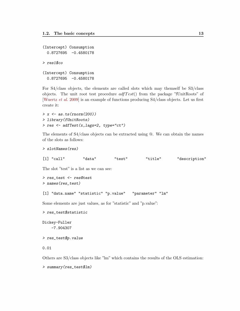
For S4/class objects, the elements are called slots which may themself be S3/class
objects. The unit root test procedure adfTest() from the package ”fUnitRoots” of
[Wuertz et al. 2009] is an example of functions producing S4/class objects. Let us first
create it:
> x <- as.ts(rnorm(200))
> library(fUnitRoots)
> res <- adfTest(x,lags=2, type="ct")
The elements of S4/class objects can be extracted using @. We can obtain the names
of the slots as follows:
> slotNames(res)
[1] "call" "data" "test" "title" "description"
The slot ”test” is a list as we can see:
> res_test <- res@test
> names(res_test)
[1] "data.name" "statistic" "p.value" "parameter" "lm"
Some elements are just values, as for ”statistic” and ”p.value”:
> res_test$statistic
Dickey-Fuller
-7.904307
> res_test$p.value
0.01
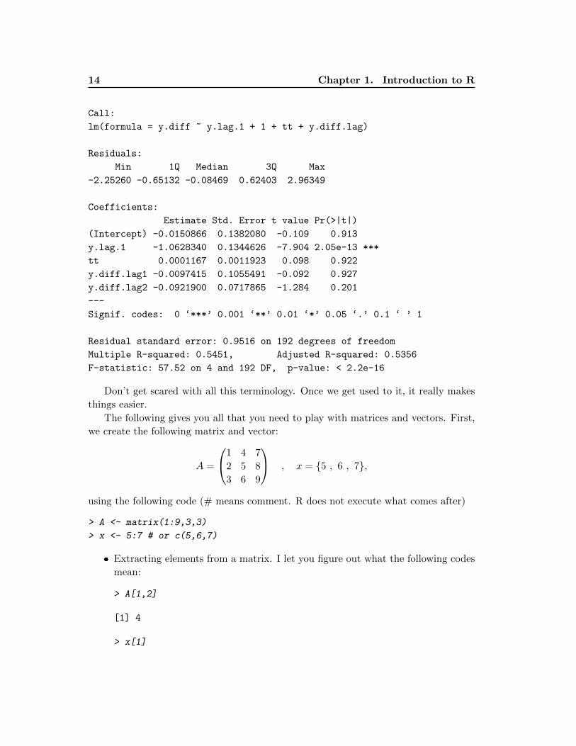
Others are S3/class objects like ”lm” which contains the results of the OLS estimation:
> summary(res_test$lm)
14 Chapter 1. Introduction to R
Call:
lm(formula = y.diff ~ y.lag.1 + 1 + tt + y.diff.lag)
Residuals:
Min 1Q Median 3Q Max
-2.25260 -0.65132 -0.08469 0.62403 2.96349
Coefficients:
Estimate Std. Error t value Pr(>|t|)
(Intercept) -0.0150866 0.1382080 -0.109 0.913
y.lag.1 -1.0628340 0.1344626 -7.904 2.05e-13 ***
tt 0.0001167 0.0011923 0.098 0.922
y.diff.lag1 -0.0097415 0.1055491 -0.092 0.927
y.diff.lag2 -0.0921900 0.0717865 -1.284 0.201
---
Signif. codes: 0 ‘***’ 0.001 ‘**’ 0.01 ‘*’ 0.05 ‘.’ 0.1 ‘ ’ 1
Residual standard error: 0.9516 on 192 degrees of freedom
Multiple R-squared: 0.5451, Adjusted R-squared: 0.5356
F-statistic: 57.52 on 4 and 192 DF, p-value: < 2.2e-16
Don’t get scared with all this terminology. Once we get used to it, it really makes
things easier.
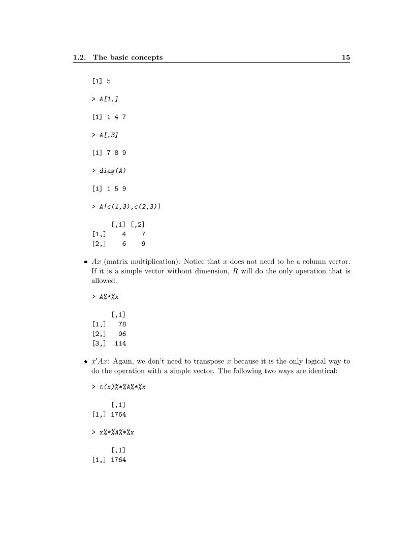
The following gives you all that you need to play with matrices and vectors. First,
we create the following matrix and vector:
A =
1 4 7
2 5 8
3 6 9
, x = {5 , 6 , 7},
using the following code (# means comment. R does not execute what comes after)
> A <- matrix(1:9,3,3)
> x <- 5:7 # or c(5,6,7)
� Extracting elements from a matrix. I let you figure out what the following codes
mean:
> A[1,2]
[1] 4
> x[1]
1.2. The basic concepts 15
[1] 5
> A[1,]
[1] 1 4 7
> A[,3]
[1] 7 8 9
> diag(A)
[1] 1 5 9
> A[c(1,3),c(2,3)]
[,1] [,2]
[1,] 4 7
[2,] 6 9
� Ax (matrix multiplication): Notice that x does not need to be a column vector.
If it is a simple vector without dimension, R will do the only operation that is
allowed.
> A%*%x
[,1]
[1,] 78
[2,] 96
[3,] 114
� x′Ax: Again, we don’t need to transpose x because it is the only logical way to
do the operation with a simple vector. The following two ways are identical:
> t(x)%*%A%*%x
[,1]
[1,] 1764
> x%*%A%*%x
[,1]
[1,] 1764
16 Chapter 1. Introduction to R
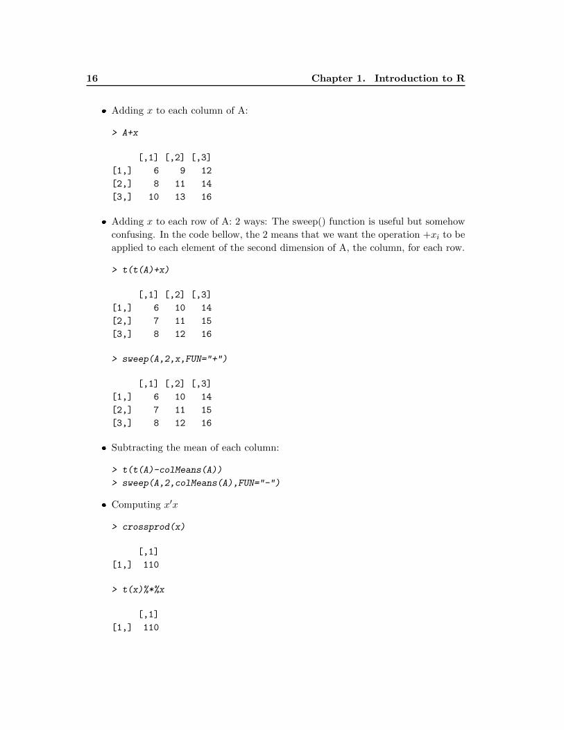
� Adding x to each column of A:
> A+x
[,1] [,2] [,3]
[1,] 6 9 12
[2,] 8 11 14
[3,] 10 13 16
� Adding x to each row of A: 2 ways: The sweep() function is useful but somehow
confusing. In the code bellow, the 2 means that we want the operation +xi to be
applied to each element of the second dimension of A, the column, for each row.
> t(t(A)+x)
[,1] [,2] [,3]
[1,] 6 10 14
[2,] 7 11 15
[3,] 8 12 16
> sweep(A,2,x,FUN="+")
[,1] [,2] [,3]
[1,] 6 10 14
[2,] 7 11 15
[3,] 8 12 16
� Subtracting the mean of each column:
> t(t(A)-colMeans(A))
> sweep(A,2,colMeans(A),FUN="-")
� Computing x′x
> crossprod(x)
[,1]
[1,] 110
> t(x)%*%x
[,1]
[1,] 110
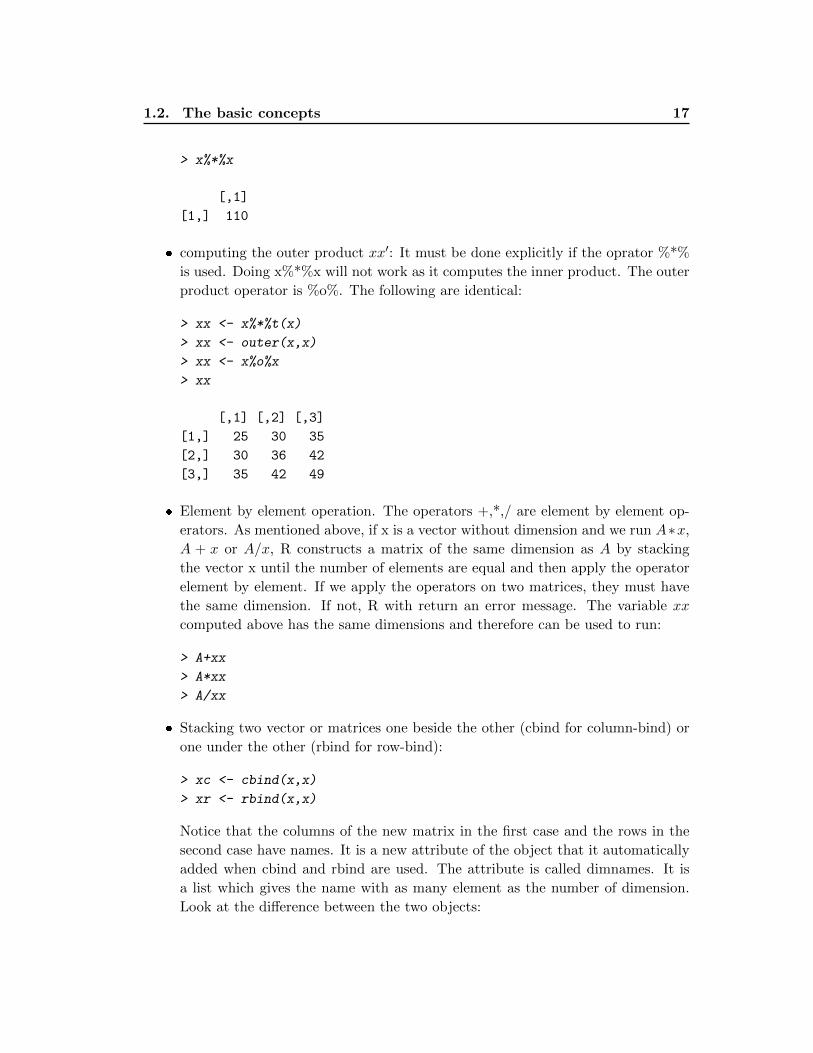
1.2. The basic concepts 17
> x%*%x
[,1]
[1,] 110
� computing the outer product xx′: It must be done explicitly if the oprator %*%
is used. Doing x%*%x will not work as it computes the inner product. The outer
product operator is %o%. The following are identical:
> xx <- x%*%t(x)
> xx <- outer(x,x)
> xx <- x%o%x
> xx
[,1] [,2] [,3]
[1,] 25 30 35
[2,] 30 36 42
[3,] 35 42 49
� Element by element operation. The operators +,*,/ are element by element op-
erators. As mentioned above, if x is a vector without dimension and we run A∗x,
A + x or A/x, R constructs a matrix of the same dimension as A by stacking
the vector x until the number of elements are equal and then apply the operator
element by element. If we apply the operators on two matrices, they must have
the same dimension. If not, R with return an error message. The variable xx
computed above has the same dimensions and therefore can be used to run:
> A+xx
> A*xx
> A/xx
� Stacking two vector or matrices one beside the other (cbind for column-bind) or
one under the other (rbind for row-bind):
> xc <- cbind(x,x)
> xr <- rbind(x,x)
Notice that the columns of the new matrix in the first case and the rows in the
second case have names. It is a new attribute of the object that it automatically
added when cbind and rbind are used. The attribute is called dimnames. It is
a list which gives the name with as many element as the number of dimension.
Look at the difference between the two objects:
18 Chapter 1. Introduction to R
> attributes(xc)
$dim
[1] 3 2
$dimnames
$dimnames[[1]]
NULL
$dimnames[[2]]
[1] "x" "x"
> attributes(xr)
$dim
[1] 2 3
$dimnames
$dimnames[[1]]
[1] "x" "x"
$dimnames[[2]]
NULL
xc has no row names and xr has no column names.
� Adding or modifying names: matrix or data.frame?. This has nothing to do with
matrix operation but since we just saw that rows and columns can have names,
it is a good place to start. First, why would we be interested in giving names to
rows and columns? In economics, each number we are playing with are associated
with something. For example, suppose the matrix B stores the information about
the consumption habits of individuals. Suppose we have three individuals and 2
goods. Here is one way to create it:
> B <- matrix(c(200,100,150,150,100,200),2,3)
> dimnames(B) <- list(c("Book","Beer"),c("John","James","Bill"))
> B
John James Bill
Book 200 150 100
Beer 100 150 200
1.2. The basic concepts 19
A data.frame is another class of objects that is used to store data. It has different
attributes than matrices which implies that some operators or methods may work
with matrices and not with data.frame and vice versa. Since data.frame objects
are also lists, we start by introducing that particular object. A list is a collection
of almost everything you can think of. Here is an example:
> Pierre = list(address = "UofW Waterloo",
+ Inventory=c("Computer", "Coffee Maker","Books"),
+ LuckyNumbers = c(2,5,6,733,44))
You can extract the element of a list with $ as seen above or with [[i]] for the
value of the ith element of the list or [1] for the element with the name:
> Pierre[1] # This is still a list
$address
[1] "UofW Waterloo"
> Pierre[[1]] # this if the object of the list
[1] "UofW Waterloo"
> Pierre$addr
[1] "UofW Waterloo"
You can add things to the list like:
> Pierre$Mydata <- B
> Pierre$Mydata
John James Bill
Book 200 150 100
Beer 100 150 200
A data.frame is more restrictive because it requires the elements to be vectors
with the same number of elements. In the following example, I generate data
randomly and store them in a data.frame object:
> set.seed(100)
> X1 <- rnorm(100,mean=200,sd=50)
> X2 <- rnorm(100,mean=500,sd=25)
> Data <- data.frame(Consumption=X1, Income=X2)
> is(Data)
20 Chapter 1. Introduction to R
[1] "data.frame" "list" "oldClass" "vector"
The is() function shows the inheritance of the object. The ”list” means that we
can treat the object as a list. We can then extract the Income using Data$Income
or Data[[2]]. The is() also tells us that the data.frame can be treated as a vector.
We can then do operation on a data.frame. For example, we can rescale the Data
as follows:
> Data <- Data/100
However, we cannot do matrix operations because the inheritance does not include
”matrix”. If we want, we can transform a data.frame to a matrix:
> Data <- as.matrix(Data)
We can also change it back to a data.frame:
> Data <- as.data.frame(Data)
� Time series object: We can create a time series object with ts(). That object
has an attribute called tsp that gives information about the first and last dates
and the frequency of the data. For example, we can define the above Data as a
quarterly time series starting the first quarter of 1970:
> tsData <- ts(Data,start=c(1970,1),freq=4)
> is(tsData)
[1] "mts" "matrix" "ts" "array" "structure"
[6] "oldClass" "vector" "otherornull"
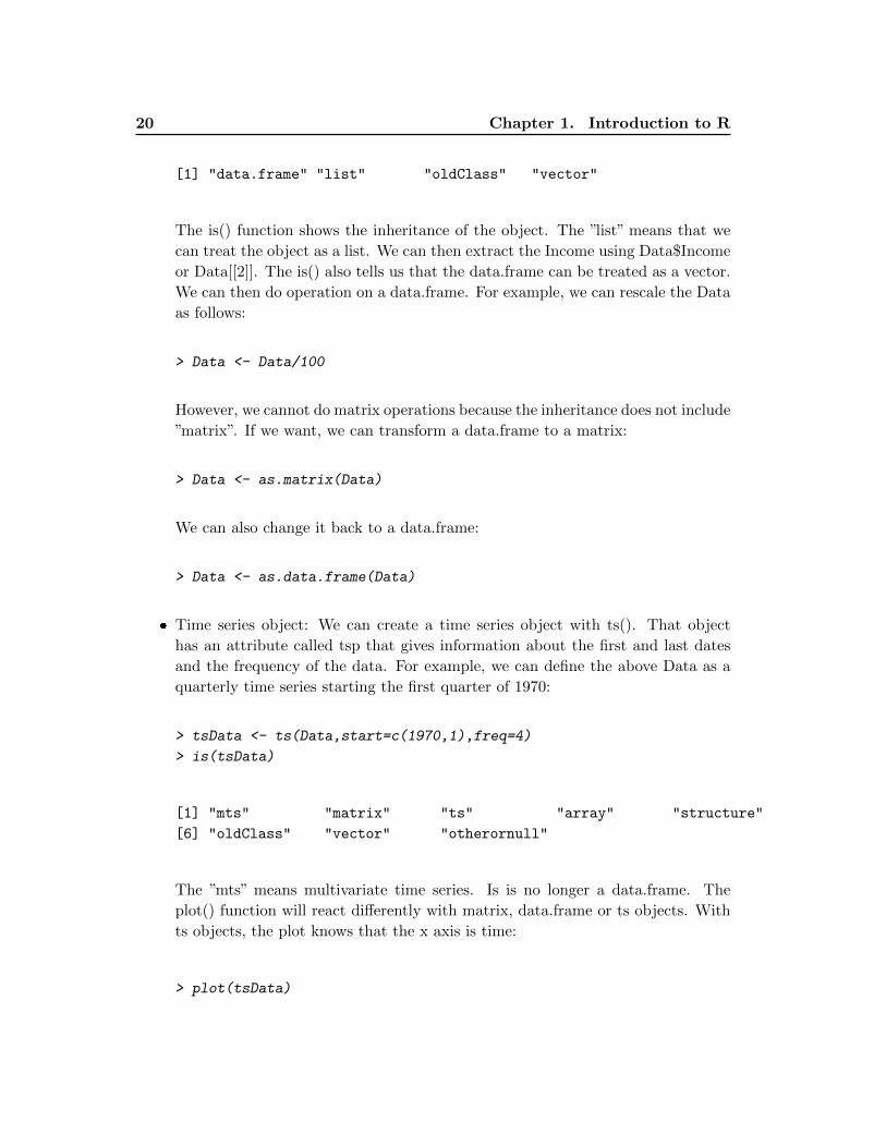
The ”mts” means multivariate time series. Is is no longer a data.frame. The
plot() function will react differently with matrix, data.frame or ts objects. With
ts objects, the plot knows that the x axis is time:
> plot(tsData)
1.2. The basic concepts 21
1.0
2.0
3.0
Con
sum
ptio
n
4.6
5.0
5.4
1970 1975 1980 1985 1990 1995
Inco
me
Time
tsData
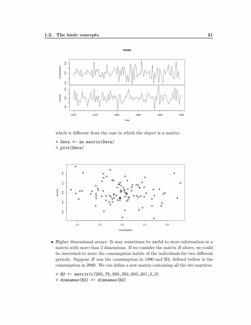
which is different from the case in which the object is a matrix:
> Data <- as.matrix(Data)
> plot(Data)
●
●
●
●
●
●
●
●
●
●
●●
●
●
●
●
●
●●
●
●
●
●
●
●
●
●
●
●
●
●
●
●
●
●
●
●
●
●
●
●
●
●
●
●●
●●
●
●
●
●
● ●
●
●
● ●
●●
●
●
●
●
●
●
●
●
●
●
●
●
●
●
●
●
●
●
●
●
●
●
●
●
●●
●
●
●
●
● ●
●
●
●
●
●
●
●
●
1.0 1.5 2.0 2.5 3.0
4.6
4.8
5.0
5.2
5.4
Consumption
Inco
me
� Higher dimensional arrays: It may sometimes be useful to store information in a
matrix with more than 2 dimensions. If we consider the matrix B above, we could
be interested to store the consumption habits of the individuals for two different
periods. Suppose B was the consumption in 1990 and B2, defined bellow is the
consumption in 2000. We can define a new matrix containing all the two matrices.
> B2 <- matrix(c(250,75,300,250,500,20),2,3)
> dimnames(B2) <- dimnames(B2)
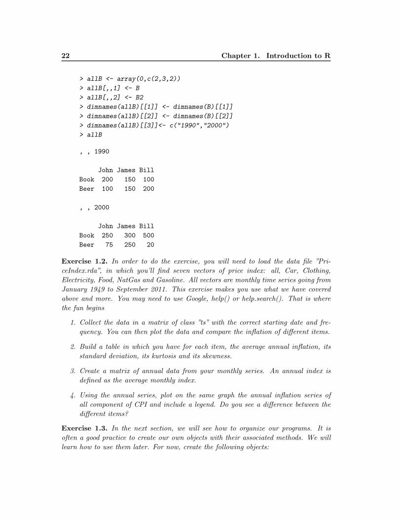
22 Chapter 1. Introduction to R
> allB <- array(0,c(2,3,2))
> allB[,,1] <- B
> allB[,,2] <- B2
> dimnames(allB)[[1]] <- dimnames(B)[[1]]
> dimnames(allB)[[2]] <- dimnames(B)[[2]]
> dimnames(allB)[[3]]<- c("1990","2000")
> allB
, , 1990
John James Bill
Book 200 150 100
Beer 100 150 200
, , 2000
John James Bill
Book 250 300 500
Beer 75 250 20
Exercise 1.2. In order to do the exercise, you will need to load the data file ”Pri-
ceIndex.rda”, in which you’ll find seven vectors of price index: all, Car, Clothing,
Electricity, Food, NatGas and Gasoline. All vectors are monthly time series going from
January 1949 to September 2011. This exercise makes you use what we have covered
above and more. You may need to use Google, help() or help.search(). That is where
the fun begins
1. Collect the data in a matrix of class ”ts” with the correct starting date and fre-
quency. You can then plot the data and compare the inflation of different items.
2. Build a table in which you have for each item, the average annual inflation, its
standard deviation, its kurtosis and its skewness.
3. Create a matrix of annual data from your monthly series. An annual index is
defined as the average monthly index.
4. Using the annual series, plot on the same graph the annual inflation series of
all component of CPI and include a legend. Do you see a difference between the
different items?
Exercise 1.3. In the next section, we will see how to organize our programs. It is
often a good practice to create our own objects with their associated methods. We will
learn how to use them later. For now, create the following objects:
1.3. Organizing our programs 23
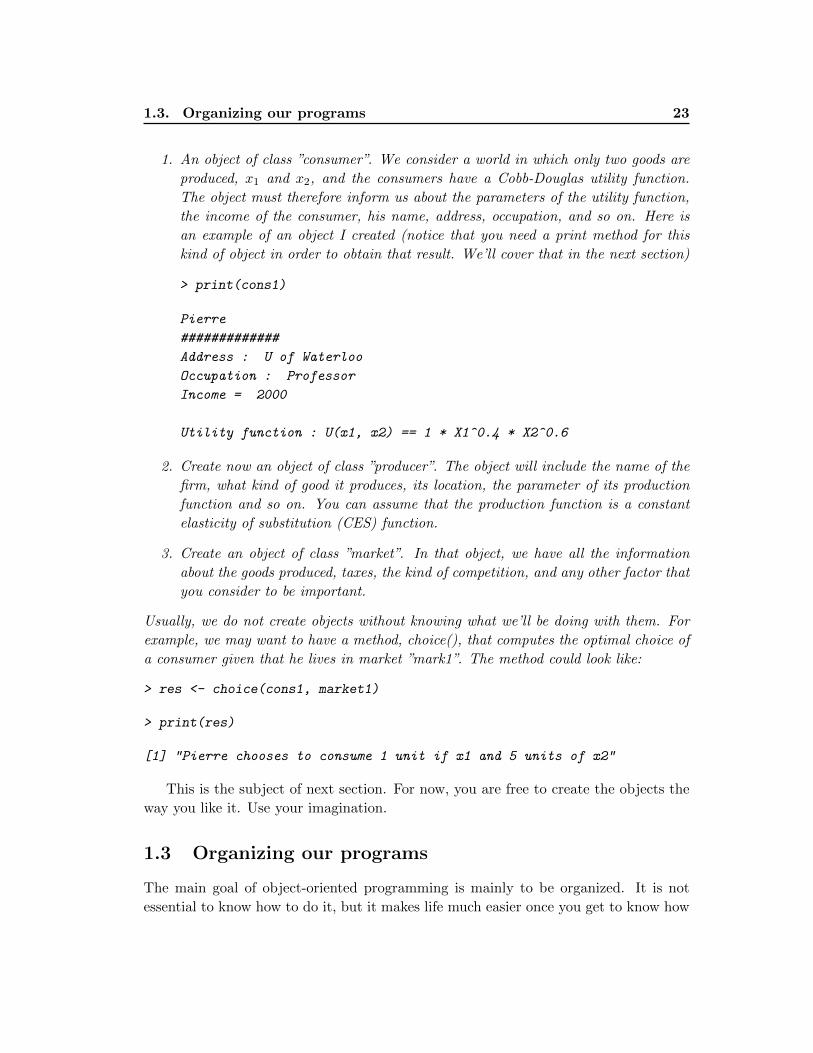
1. An object of class ”consumer”. We consider a world in which only two goods are
produced, x1 and x2, and the consumers have a Cobb-Douglas utility function.
The object must therefore inform us about the parameters of the utility function,
the income of the consumer, his name, address, occupation, and so on. Here is
an example of an object I created (notice that you need a print method for this
kind of object in order to obtain that result. We’ll cover that in the next section)
> print(cons1)
Pierre
#############
Address : U of Waterloo
Occupation : Professor
Income = 2000
Utility function : U(x1, x2) == 1 * X1^0.4 * X2^0.6
2. Create now an object of class ”producer”. The object will include the name of the
firm, what kind of good it produces, its location, the parameter of its production
function and so on. You can assume that the production function is a constant
elasticity of substitution (CES) function.
3. Create an object of class ”market”. In that object, we have all the information
about the goods produced, taxes, the kind of competition, and any other factor that
you consider to be important.
Usually, we do not create objects without knowing what we’ll be doing with them. For
example, we may want to have a method, choice(), that computes the optimal choice of
a consumer given that he lives in market ”mark1”. The method could look like:
> res <- choice(cons1, market1)
> print(res)
[1] "Pierre chooses to consume 1 unit if x1 and 5 units of x2"
This is the subject of next section. For now, you are free to create the objects the
way you like it. Use your imagination.
1.3 Organizing our programs
The main goal of object-oriented programming is mainly to be organized. It is not
essential to know how to do it, but it makes life much easier once you get to know how
24 Chapter 1. Introduction to R
to do it. Just take for example the comment at the end of Exercise 1.3. For solving the
consumer problem, you could write a program like the following which I would consider
the least organized approach (keep in mind that many things I write here are a matter
of opinion or taste. If you don’t agree, speak up!):
> # We consider the consumer "cons1" created in the
> # previous section
> p1 <- 5
> p2 <- 10
> a1 <- .4
> a2 <- .6
> Y <- 2000
> x1 <- a1*Y/p1
> x2 <- a2*Y/p2
> print(x1)
[1] 160
> print(x2)
[1] 120
There are several problem with that approach. If you want to do it for another con-
sumer, you need to rewrite all the lines with different parameter values. Remember
that one way to minimize the risk of errors is to have a shorter programs. It is simple
arithmetics. Also, you need to know the solution of the utility maximization in order
to compute the solution. What if you have a totally new utility function?
I am going to the extreme here because I believe it is the best way to learn. Or
course, it is not always optimal to spend time being organized for everything we com-
pute. For example, if you only have to do it once for an assignment and you will never
solve another consumer problem in the future because you hate microeconomics, then
it is probably the best way to compute it. However, it is a good practice to be more or-
ganized especially when the complexity of the problem we are trying to solve increases.
I am presenting you my way of programming. It is not the only way. You are free to
choose your own way.
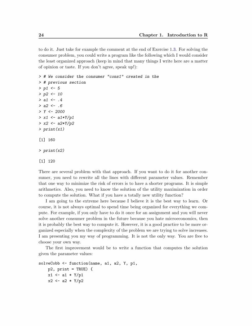
The first improvement would be to write a function that computes the solution
given the parameter values:
solveCobb <- function(name, a1, a2, Y, p1,
p2, print = TRUE) {
x1 <- a1 * Y/p1
x2 <- a2 * Y/p2
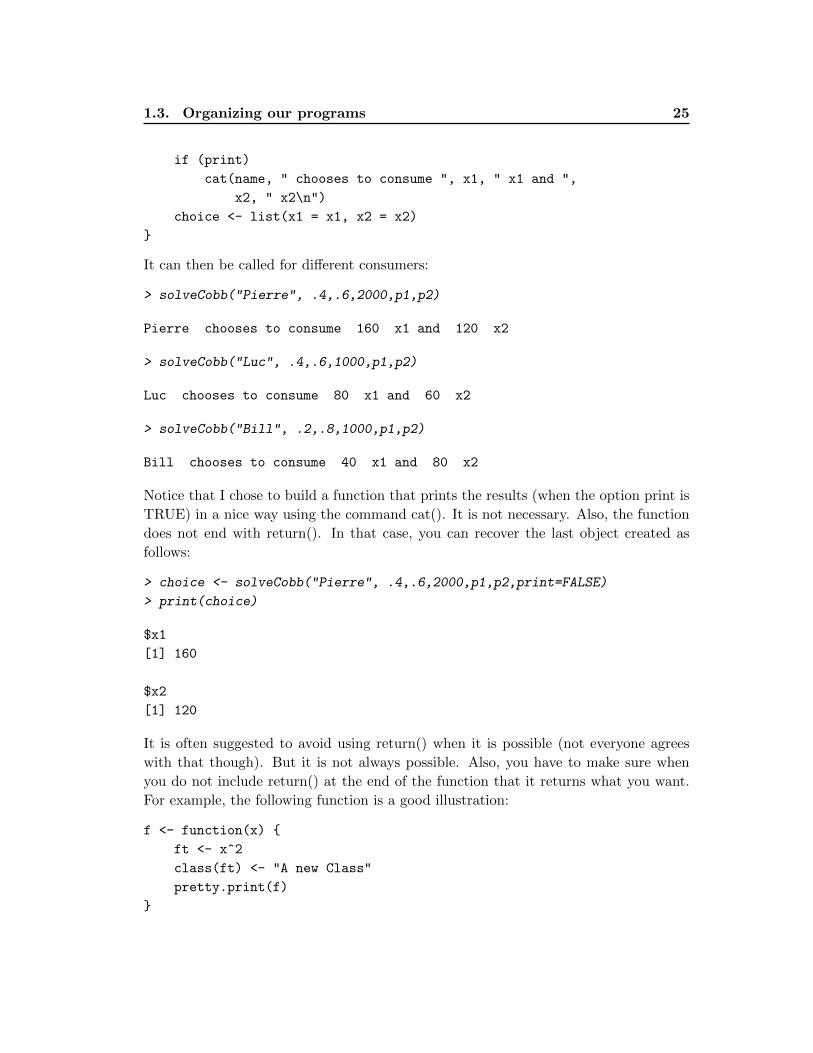
1.3. Organizing our programs 25
if (print)
cat(name, " chooses to consume ", x1, " x1 and ",
x2, " x2\n")
choice <- list(x1 = x1, x2 = x2)
}
It can then be called for different consumers:
> solveCobb("Pierre", .4,.6,2000,p1,p2)
Pierre chooses to consume 160 x1 and 120 x2
> solveCobb("Luc", .4,.6,1000,p1,p2)
Luc chooses to consume 80 x1 and 60 x2
> solveCobb("Bill", .2,.8,1000,p1,p2)
Bill chooses to consume 40 x1 and 80 x2
Notice that I chose to build a function that prints the results (when the option print is
TRUE) in a nice way using the command cat(). It is not necessary. Also, the function
does not end with return(). In that case, you can recover the last object created as
follows:
> choice <- solveCobb("Pierre", .4,.6,2000,p1,p2,print=FALSE)
> print(choice)
$x1
[1] 160
$x2
[1] 120
It is often suggested to avoid using return() when it is possible (not everyone agrees
with that though). But it is not always possible. Also, you have to make sure when
you do not include return() at the end of the function that it returns what you want.
For example, the following function is a good illustration:
f <- function(x) {
ft <- x^2
class(ft) <- "A new Class"
pretty.print(f)
}
26 Chapter 1. Introduction to R
$text.tidy
[1] "f <- function(x) {\n ft <- x^2\n class(ft) <- \"A new Class\"\n pretty.print(f)\n}"
$text.mask
[1] "f <- function(x) {\n ft <- x^2\n class(ft) <- \"A new Class\"\n pretty.print(f)\n}"
$begin.comment
[1] ".BeGiN_TiDy_IdEnTiFiEr_HaHaHa"
$end.comment
[1] ".HaHaHa_EnD_TiDy_IdEnTiFiEr"
So it returns the class of the object instead of the object itself. In that case, you
have to end the function with return(r). Another improvement would be to store the
information of a particular consumer in a variable (like in Exercise 1.3) and use that
variable as argument for solveCobb(). Let us first create the consumer:
> pierre <- list(a1=.4,a2=.6,Y=2000,name="Pierre")
> luc <- list(a1=.2,a2=.8,Y=1000,name="Luc")
Then, we have to adapt the function solveCobb():
solveCobb <- function(cons, p1, p2, print = TRUE) {
x1 <- cons$a1 * cons$Y/p1
x2 <- cons$a2 * cons$Y/p2
if (print)
cat(cons$name, " chooses to consume ", x1,
" x1 and ", x2, " x2\n")
choice <- list(x1 = x1, x2 = x2)
}
> solveCobb(pierre,p1,p2)
Pierre chooses to consume 160 x1 and 120 x2
> solveCobb(luc,p1,p2)
Luc chooses to consume 40 x1 and 80 x2
I am still not satisfied with the above. Creating the consumers using a list() used by
solveCobb may not work if we misspell the name of the variables or if we forget to
define one. In general, when you want to use an object inside a function which respects
a certain structure, it is better to have another function that creates that object. In C
1.3. Organizing our programs 27
or C++, we call these kind of functions the constructors. I like things to be as general
as possible when I write programs so that it can easily be adapted to other realities.
Here is a consumer constructor that I propose:
consumer <- function(name = NULL, para,
Y, utility = c("Cobb", "Linear", "Leontief", "Subsistence")) {
utility <- match.arg(utility)
if (utility == "Subsistence") {
x01 = para[3]
x02 = para[4]
} else {
x01 = NULL
x02 = NULL
}
# Cobb = x1^a1*x2^a2, Linear = a1*x1 + a2*x2
# Leontief = min(a1*x2, a2*x2), Subsistence =
# (x1-x01)^a1(x2-x02)^a2
# para = c(a1, a2, x10, x20)
list(name = name, a1 = para[1], a2 = para[2], x01 = x01,
x02 = x02, Y = Y, utility = utility)
}
Notice that utility can take more than one values. The first line in the function is
to make sure that what we write is among the choices. It also allow us to use the
first letters when there is no ambiguity. For example, we can write utility=”C” or
utility=”Li”, but not utility=”L”. The first choice in the list is the default value. We
can then proceed as follows:
> pierre <- consumer("pierre",c(.4,.6),2000)
> solveCobb(pierre,p1,p1)
pierre chooses to consume 160 x1 and 240 x2
Exercise 1.4. Write three functions for the last three utility functions in the list of con-
sumer() that solves the consumer problem. You can call them solveLinear(), solveLeon-
tief() and solveSubsistence().
Exercise 1.5. Write a function that creates an object ”market” that includes the price
of the two goods and the taxe imposed on each one (t1 and t2). Then adapt the solve
functions so that they only take the market and consumer objects as arguments (ex.
solveCobb(cons1, market1, print=T))
28 Chapter 1. Introduction to R
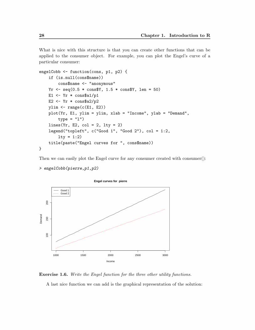
What is nice with this structure is that you can create other functions that can be
applied to the consumer object. For example, you can plot the Engel’s curve of a
particular consumer:
engelCobb <- function(cons, p1, p2) {
if (is.null(cons$name))
cons$name <- "anonymous"
Yr <- seq(0.5 * cons$Y, 1.5 * cons$Y, len = 50)
E1 <- Yr * cons$a1/p1
E2 <- Yr * cons$a2/p2
ylim <- range(c(E1, E2))
plot(Yr, E1, ylim = ylim, xlab = "Income", ylab = "Demand",
type = "l")
lines(Yr, E2, col = 2, lty = 2)
legend("topleft", c("Good 1", "Good 2"), col = 1:2,
lty = 1:2)
title(paste("Engel curves for ", cons$name))
}
Then we can easily plot the Engel curve for any consumer created with consumer():
> engelCobb(pierre,p1,p2)
1000 1500 2000 2500 3000
100
150
200
Income
Dem
and
Good 1Good 2
Engel curves for pierre
Exercise 1.6. Write the Engel function for the three other utility functions.
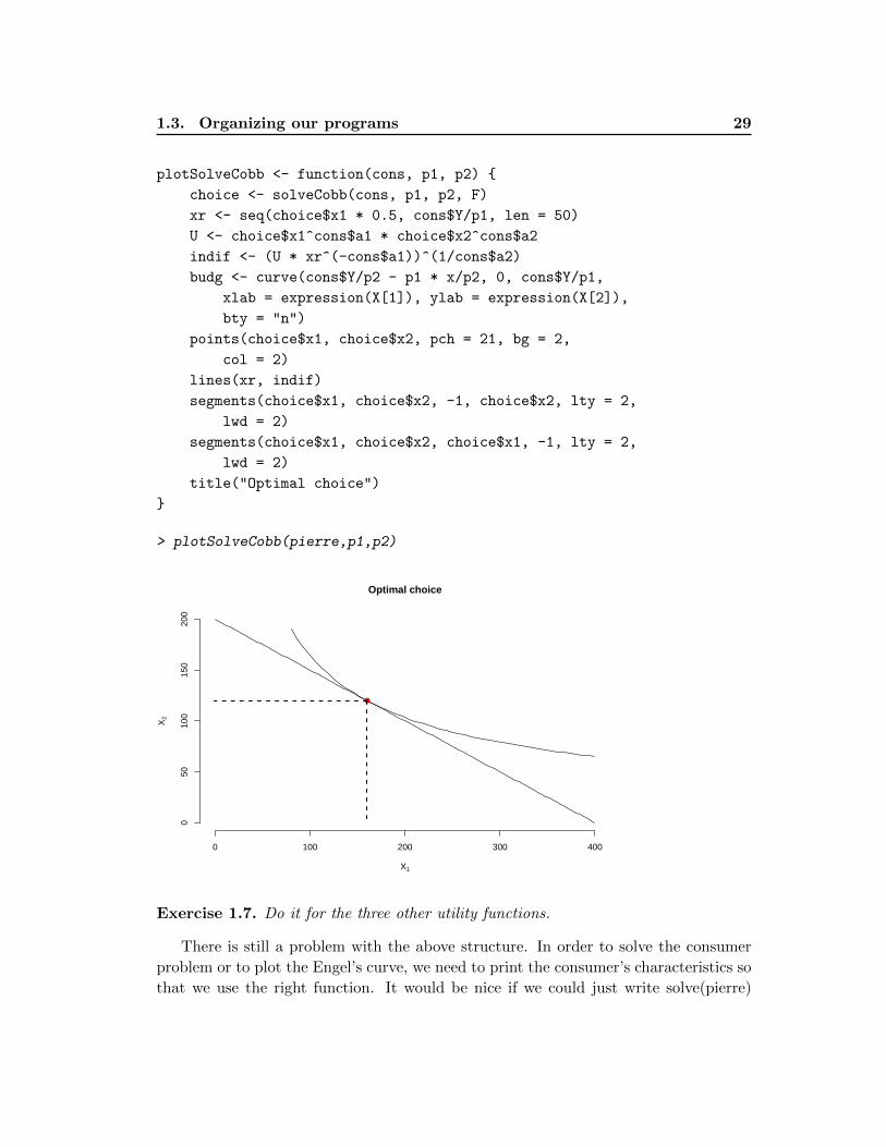
A last nice function we can add is the graphical representation of the solution:
1.3. Organizing our programs 29
plotSolveCobb <- function(cons, p1, p2) {
choice <- solveCobb(cons, p1, p2, F)
xr <- seq(choice$x1 * 0.5, cons$Y/p1, len = 50)
U <- choice$x1^cons$a1 * choice$x2^cons$a2
indif <- (U * xr^(-cons$a1))^(1/cons$a2)
budg <- curve(cons$Y/p2 - p1 * x/p2, 0, cons$Y/p1,
xlab = expression(X[1]), ylab = expression(X[2]),
bty = "n")
points(choice$x1, choice$x2, pch = 21, bg = 2,
col = 2)
lines(xr, indif)
segments(choice$x1, choice$x2, -1, choice$x2, lty = 2,
lwd = 2)
segments(choice$x1, choice$x2, choice$x1, -1, lty = 2,
lwd = 2)
title("Optimal choice")
}
> plotSolveCobb(pierre,p1,p2)
0 100 200 300 400
050
100
150
200
X1
X2
●
Optimal choice
Exercise 1.7. Do it for the three other utility functions.
There is still a problem with the above structure. In order to solve the consumer
problem or to plot the Engel’s curve, we need to print the consumer’s characteristics so
that we use the right function. It would be nice if we could just write solve(pierre)
30 Chapter 1. Introduction to R
plot(pierre) or Engel(pierre). We can either write a function with things like ”if
(cons$utility==”Cobb”) ... else if () ... else ...” or to use classes. I let the consumer
problem to you as an exercise at the end of the chapter. But before we’ll see how to
create objects, classes and methods using a very simple example.
1.3.1 Classes and methods for second order polynomials
Classes are a way of identifying the type of objects. We saw several classes in the previ-
ous sections such as ”ts”, ”vector”, ”numeric”. We also saw that methods such as plot()
react differently depending on the object. There is no magic here; just organization.
Suppose for example that we have an object x of class ”ts” and a simple vector y. The
reason why plot(x) and plot(y) produce different graphs is that different functions are
called. Because x is of class ts, plot(x) is in fact plot.ts(x). R looks for functions with
names ending by .ts when applied to objects of class ”ts”. It produces a time series plot
with the dates which are included inside the structure of x. Those dates exist because
x was created using the constructor ts() which always creates dates. The type of plot
is also automatically chosen to be ”l”. On the other hand, there is no specific plot()
method for regular vector. In that case, it is the function plot.default() that is called
for y. There are many plot() methods for all kind of objects. Imagine how messy it
would be to put everything inside one function plot() with a collection of ”if... else
if” everywhere. The function plot.default() works fine. So why should we modify it?
Every time we need to plot another object, we create a new function. That function
can then be tested and bugs can easily be removed.
This is what we are going to do in this section for a simple object: a second order
polynomial. A second order polynomial is defined by its 3 parameters: A, B and C:
f(x) = Ax2 +Bx+ C
We first write the constructor. It is like for the consumer constructor that we built
in the previous section. The only difference is that we want that object to belong to
a particular class that we will call ”Quadra”. This is simply done using the function
class():
Quadra <- function(a, b, c) {
if (a == 0)
stop("It is not a quadratique function;\n'a' must be different from zero")
obj <- list(a = a, b = b, c = c)
class(obj) <- "Quadra"
return(obj)
}
We can then create the polynomial f(x) = 2x2 − 4x+ 10 and print it.
1.3. Organizing our programs 31
> P1 <- Quadra(2,-4,10)
> P1
$a
[1] 2
$b
[1] -4
$c
[1] 10
attr(,"class")
[1] "Quadra"
We can see that the output from the print() method is not very nice. But because there
is no print.Quadra() function, the print.default() is used. There is a print() method for
a large number of objects. For example, if you estimate a model by OLS using lm().
The object created is of class ”lm”. There is a lot of information inside that object
(residuals, fitted values, covariance matrix of the coefficients and so on) but we don’t
want print() to show everything. Therefore, print.lm() only prints the estimates and
few other things. Let us do the same for our new object:
print.Quadra <- function(obj) {
cat("\nSecond order polynomial\n\n")
cat("F(x) = Ax^2 + Bx + C\n")
cat("with: A=", obj$a, ", B=", obj$b, ", C=", obj$c,
"\n\n")
}
Then we can try it on the object we created before (notice that just writing P1 is the
same as writing print(P1)):
> P1
Second order polynomial
F(x) = Ax^2 + Bx + C
with: A= 2 , B= -4 , C= 10
Now that we are starting to understand the idea, lets create a bunch of other methods.
The next one finds the zeros of the polynomial which could be real or complex. The
32 Chapter 1. Introduction to R
method I want to use is zeros(). However, that method does not exist in R like print().
Therefore we need to inform R of this new method (which could be use to find zeros
of any kind of function f(x) by other users ):
zeros <- function(object, ...) {
UseMethod("zeros")
}
The ”...” are required because the zeros() method applied to other type of objects may
required other arguments. We can now create our new method for the object of class
”Quadra”.
zeros.Quadra <- function(obj) {
det <- obj$b^2 - 4 * obj$a * obj$c
if (det > .Machine$double.eps) {
r1 <- (-obj$b - sqrt(det))/(2 * obj$a)
r2 <- (-obj$b + sqrt(det))/(2 * obj$a)
r <- cbind(r1, r2)
class(r) <- "zeros"
attr(r, "type") = "Real and distinct"
}
if (abs(det) <= .Machine$double.eps) {
r1 <- -obj$b/(2 * obj$a)
r <- cbind(r1, r1)
class(r) <- "zeros"
attr(r, "type") = "Real and identical"
}
if (det < -.Machine$double.eps) {
det <- sqrt(-det)/(2 * obj$a)
r1 <- -obj$b/(2 * obj$a) - det * (0+1i)
r2 <- -obj$b/(2 * obj$a) + det * (0+1i)
r <- cbind(r1, r2)
class(r) <- "zeros"
attr(r, "type") = "Complexe"
}
return(r)
}
We will discuss the content of the function in class. Notice that the function produces
objects of class ”zeros”. We can then create a print method for that class of objects.
print.zeros <- function(obj) {
n <- length(obj)
1.3. Organizing our programs 33
cat("\nType of zeros: ", attr(obj, "type"), "\n\n")
for (i in 1:n) cat("Zero[", i, "] = ", obj[i],
"\n")
cat("\n")
}
We can then apply the method to the polynomial P1 and print it directly:
> zeros(P1)
Type of zeros: Complexe
Zero[ 1 ] = 1-2i
Zero[ 2 ] = 1+2i
Lets create another polynomial with real zeros:
> P2 <- Quadra(-4,2,10)
> zeros(P2)
Type of zeros: Real and distinct
Zero[ 1 ] = 1.850781
Zero[ 2 ] = -1.350781
The next method computes the stationary point (max or min). For that, I use the
existing method solve() and the object produced is of class ”solve.Quadra”. I then
create a print method for that new object.
solve.Quadra <- function(obj) {
x <- -obj$b/(2 * obj$a)
f <- obj$a * x^2 + obj$b * x + obj$c
if (obj$a > 0)
what <- "min" else what <- "max"
ans <- list(x = x, f = f, what = what)
class(ans) <- "solve.Quadra"
return(ans)
}
print.solve.Quadra <- function(obj) {
if (obj$what == "min")
mes <- "\nThe polynomial has a minimum at " else mes <- "\nThe polynomial has a maximum at "
cat(mes, "x = ", obj$x, "\n")
cat("At that point, f(x) = ", obj$f, "\n\n")
}
34 Chapter 1. Introduction to R
Lets try them:
> solve(P1)
The polynomial has a minimum at x = 1
At that point, f(x) = 8
> solve(P2)
The polynomial has a maximum at x = 0.25
At that point, f(x) = 10.25
Notice that I did not use the generic function solve() as it should be. If you look at
help(solve), it says that it is a generic function for solving Ax = b and the inputs are A
and b. In the package numericalecon I created on RForge, I had to change the function
name to solveP() (for solve polynomial) because we are not allowed to use existing
generic functions with different inputs.
The following shows one nice thing we can do. We want to create a binary operator
that will allow us to add two polynomials. First we need to create the function:
addQuadra <- function(Q1, Q2) {
if (class(Q1) != "Quadra" | class(Q2) != "Quadra")
stop("This operator can only be applied to\nobjects of class Quadra")
a <- Q1$a + Q2$a
b <- Q1$b + Q2$b
c <- Q1$c + Q2$c
Quadra(a, b, c)
}
Then we create the binary operator:
> "%+%" <- function(Q1,Q2) addQuadra(Q1,Q2)
We can then create a third polynomial which is the sum of the first two:
> P3 <- P1%+%P2
> solve(P3)
The polynomial has a maximum at x = -0.5
At that point, f(x) = 20.5
> zeros(P3)
1.3. Organizing our programs 35
Type of zeros: Real and distinct
Zero[ 1 ] = 2.701562
Zero[ 2 ] = -3.701562
I conclude this section with the following two methods. We’ll discuss them in class if
we have time.
plot.Quadra <- function(obj, from = NULL,
to = NULL) {
f <- function(x) obj$a * x^2 + obj$b * x + obj$c
res <- solve(obj)
if (is.null(from) | is.null(to)) {
from <- res$x - 4
to <- res$x + 4
}
if (res$what == "min") {
d <- max(f(to), f(from)) - res$f
mes <- paste("Min=(", round(res$x, 2), ", ",
round(res$f, 2), ")", sep = "")
}
if (res$what == "max") {
mes <- paste("Max=(", round(res$x, 2), ", ",
round(res$f, 2), ")", sep = "")
d <- res$f - min(f(to), f(from))
}
curve(f, from, to, xlab = "X", ylab = "f(X)")
if (obj$b > 0 & obj$c > 0)
title(substitute(f(X) == a * X^2 + b * X +
c, obj))
if (obj$b < 0 & obj$c > 0)
title(substitute(f(X) == a * X^2 - b2 * X +
c, c(obj, b2 = -obj$b)))
if (obj$b > 0 & obj$c < 0)
title(substitute(f(X) == a * X^2 + b * X -
c2, c(obj, c2 = -obj$c)))
if (obj$b == 0 & obj$c > 0)
title(substitute(f(X) == a * X^2 + c, obj))
36 Chapter 1. Introduction to R
if (obj$b == 0 & obj$c < 0)
title(substitute(f(X) == a * X^2 - c2, c(obj,
c2 = -obj$c)))
if (obj$c == 0 & obj$b > 0)
title(substitute(f(X) == a * X^2 + b * x, obj))
if (obj$c == 0 & obj$b < 0)
title(substitute(f(X) == a * X^2 - b2 * x,
c(obj, b2 = -obj$b)))
points(res$x, res$f, col = 3, cex = 0.8, pch = 21,
bg = 3)
if (res$what == "min") {
text(res$x, res$f + 0.2 * d, mes)
arrows(res$x, res$f + 0.18 * d, res$x, res$f)
} else {
text(res$x, res$f - 0.2 * d, mes)
arrows(res$x, res$f - 0.18 * d, res$x, res$f)
}
z <- zeros(obj)
if (attr(z, "type") == "Real and distinct") {
points(z[1], 0, col = 2, cex = 0.8, pch = 21,
bg = 2)
points(z[2], 0, col = 2, cex = 0.8, pch = 21,
bg = 2)
r1 <- paste(round(min(z), 2))
r2 <- paste(round(max(z), 2))
if (res$what == "min") {
if (abs(res$f) > d/2)
d2 <- -d else d2 <- d
text(min(z), 0.25 * d2, r1)
text(max(z), 0.25 * d2, r2)
arrows(min(z), 0.23 * d2, min(z), 0)
arrows(max(z), 0.23 * d2, max(z), 0)
} else {
if (abs(res$f) > d/2)
d2 <- -d else d2 <- d
text(min(z), -0.25 * d2, r1)
text(max(z), -0.25 * d2, r2)
arrows(min(z), -0.23 * d2, min(z), 0)

1.3. Organizing our programs 37
arrows(max(z), -0.23 * d2, max(z), 0)
}
}
if (attr(z, "type") != "Complexe" | attr(z, "type") ==
"Real and identical")
abline(h = 0)
}
summary.Quadra <- function(obj) {
print(obj)
print(zeros(obj))
print(solve(obj))
}
Let us test them:
> summary(P1)
Second order polynomial
F(x) = Ax^2 + Bx + C
with: A= 2 , B= -4 , C= 10
Type of zeros: Complexe
Zero[ 1 ] = 1-2i
Zero[ 2 ] = 1+2i
The polynomial has a minimum at x = 1
At that point, f(x) = 8
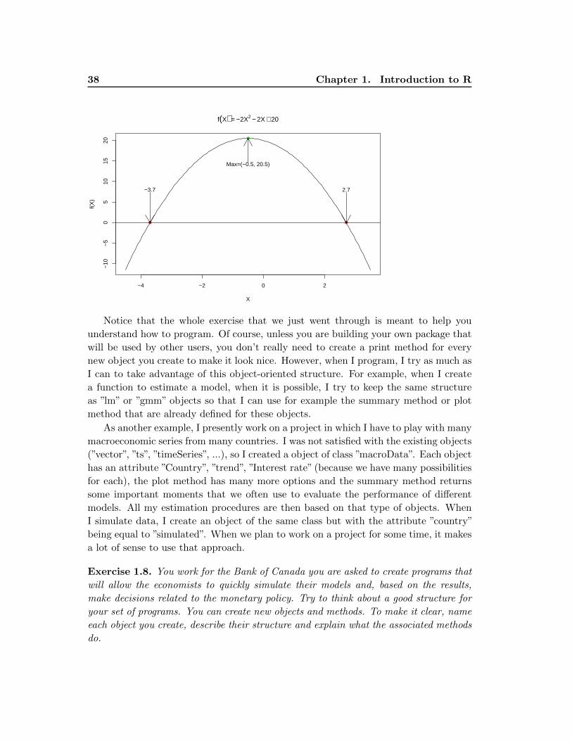
> plot(P3)
38 Chapter 1. Introduction to R
−4 −2 0 2
−10
−5
05
1015
20
X
f(X
)
f(X) = −2X2 − 2X + 20
●
Max=(−0.5, 20.5)
●●
−3.7 2.7
Notice that the whole exercise that we just went through is meant to help you
understand how to program. Of course, unless you are building your own package that
will be used by other users, you don’t really need to create a print method for every
new object you create to make it look nice. However, when I program, I try as much as
I can to take advantage of this object-oriented structure. For example, when I create
a function to estimate a model, when it is possible, I try to keep the same structure
as ”lm” or ”gmm” objects so that I can use for example the summary method or plot
method that are already defined for these objects.
As another example, I presently work on a project in which I have to play with many
macroeconomic series from many countries. I was not satisfied with the existing objects
(”vector”, ”ts”, ”timeSeries”, ...), so I created a object of class ”macroData”. Each object
has an attribute ”Country”, ”trend”, ”Interest rate” (because we have many possibilities
for each), the plot method has many more options and the summary method returns
some important moments that we often use to evaluate the performance of different
models. All my estimation procedures are then based on that type of objects. When
I simulate data, I create an object of the same class but with the attribute ”country”
being equal to ”simulated”. When we plan to work on a project for some time, it makes
a lot of sense to use that approach.
Exercise 1.8. You work for the Bank of Canada you are asked to create programs that
will allow the economists to quickly simulate their models and, based on the results,
make decisions related to the monetary policy. Try to think about a good structure for
your set of programs. You can create new objects and methods. To make it clear, name
each object you create, describe their structure and explain what the associated methods
do.
1.4. Programming efficiently 39
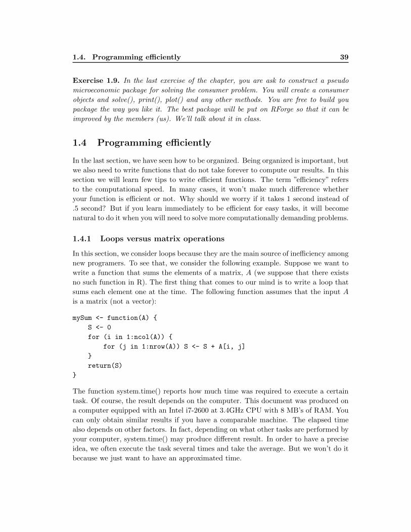
Exercise 1.9. In the last exercise of the chapter, you are ask to construct a pseudo
microeconomic package for solving the consumer problem. You will create a consumer
objects and solve(), print(), plot() and any other methods. You are free to build you
package the way you like it. The best package will be put on RForge so that it can be
improved by the members (us). We’ll talk about it in class.
1.4 Programming efficiently
In the last section, we have seen how to be organized. Being organized is important, but
we also need to write functions that do not take forever to compute our results. In this
section we will learn few tips to write efficient functions. The term ”efficiency” refers
to the computational speed. In many cases, it won’t make much difference whether
your function is efficient or not. Why should we worry if it takes 1 second instead of
.5 second? But if you learn immediately to be efficient for easy tasks, it will become
natural to do it when you will need to solve more computationally demanding problems.
1.4.1 Loops versus matrix operations
In this section, we consider loops because they are the main source of inefficiency among
new programers. To see that, we consider the following example. Suppose we want to
write a function that sums the elements of a matrix, A (we suppose that there exists
no such function in R). The first thing that comes to our mind is to write a loop that
sums each element one at the time. The following function assumes that the input A
is a matrix (not a vector):
mySum <- function(A) {
S <- 0
for (i in 1:ncol(A)) {
for (j in 1:nrow(A)) S <- S + A[i, j]
}
return(S)
}
The function system.time() reports how much time was required to execute a certain
task. Of course, the result depends on the computer. This document was produced on
a computer equipped with an Intel i7-2600 at 3.4GHz CPU with 8 MB’s of RAM. You
can only obtain similar results if you have a comparable machine. The elapsed time
also depends on other factors. In fact, depending on what other tasks are performed by
your computer, system.time() may produce different result. In order to have a precise
idea, we often execute the task several times and take the average. But we won’t do it
because we just want to have an approximated time.
40 Chapter 1. Introduction to R
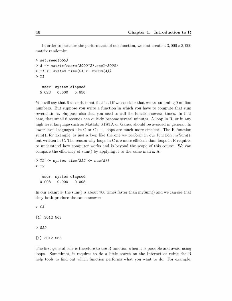
In order to measure the performance of our function, we first create a 3, 000×3, 000
matrix randomly:
> set.seed(555)
> A <- matrix(rnorm(3000^2),ncol=3000)
> T1 <- system.time(SA <- mySum(A))
> T1
user system elapsed
5.628 0.000 5.650
You will say that 6 seconds is not that bad if we consider that we are summing 9 million
numbers. But suppose you write a function in which you have to compute that sum
several times. Suppose also that you need to call the function several times. In that
case, that small 6 seconds can quickly become several minutes. A loop in R, or in any
high level language such as Matlab, STATA or Gauss, should be avoided in general. In
lower level languages like C or C++, loops are much more efficient. The R function
sum(), for example, is just a loop like the one we perform in our function mySum(),
but written in C. The reason why loops in C are more efficient than loops in R requires
to understand how computer works and is beyond the scope of this course. We can
compare the efficiency of sum() by applying it to the same matrix A:
> T2 <- system.time(SA2 <- sum(A))
> T2
user system elapsed
0.008 0.000 0.008
In our example, the sum() is about 706 times faster than mySum() and we can see that
they both produce the same answer:
> SA
[1] 3012.563
> SA2
[1] 3012.563
The first general rule is therefore to use R function when it is possible and avoid using
loops. Sometimes, it requires to do a little search on the Internet or using the R
help tools to find out which function performs what you want to do. For example,
1.4. Programming efficiently 41
suppose you want to apply a moving average on a time series to remove high frequency
fluctuations. Suppose the moving average is the following:
Xt =1
3Yt−1 +
1
3Yt +
1
3Yt+1,
with X1 = Y1 and Xn = Yn. Here Xt is the smoothed version of the series Yt. At first,
we may think that using a loop is unavoidable. Here is how we would proceed with a
loop (notice that we loose two observations):
myMA <- function(y) {
n <- length(y)
x <- rep(0, n)
x[1] <- y[1]
x[n] <- x[n]
for (i in 2:(n - 1)) x[i] <- (y[(i - 1)] + y[i] +
y[(i + 1)])/3
x <- as.ts(x)
attr(x, "tsp") <- attr(y, "tsp")
return(x)
}
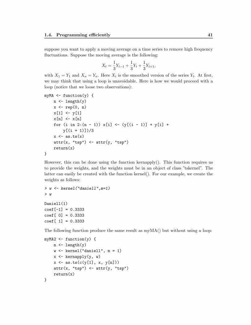
However, this can be done using the function kernapply(). This function requires us
to provide the weights, and the weights must be in an object of class ”tskernel”. The
latter can easily be created with the function kernel(). For our example, we create the
weights as follows:
> w <- kernel("daniell",m=1)
> w
Daniell(1)
coef[-1] = 0.3333
coef[ 0] = 0.3333
coef[ 1] = 0.3333
The following function produce the same result as myMA() but without using a loop:
myMA2 <- function(y) {
n <- length(y)
w <- kernel("daniell", m = 1)
x <- kernapply(y, w)
x <- as.ts(c(y[1], x, y[n]))
attr(x, "tsp") <- attr(y, "tsp")
return(x)
}
42 Chapter 1. Introduction to R
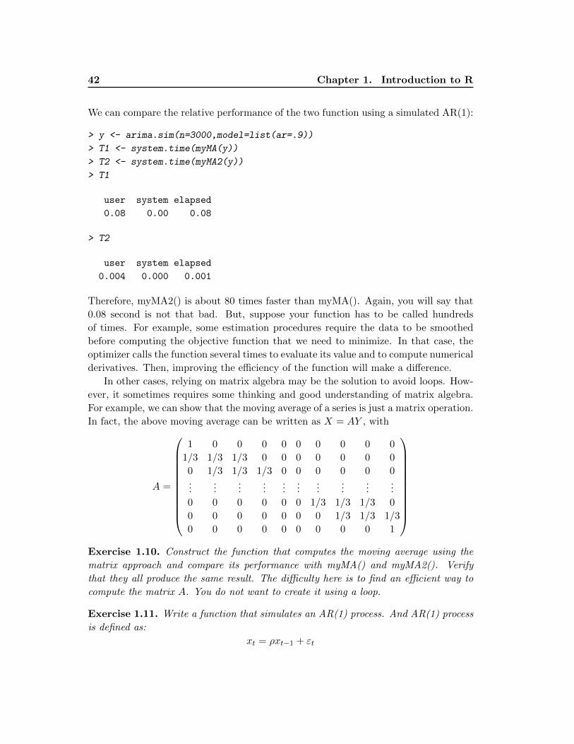
We can compare the relative performance of the two function using a simulated AR(1):
> y <- arima.sim(n=3000,model=list(ar=.9))
> T1 <- system.time(myMA(y))
> T2 <- system.time(myMA2(y))
> T1
user system elapsed
0.08 0.00 0.08
> T2
user system elapsed
0.004 0.000 0.001
Therefore, myMA2() is about 80 times faster than myMA(). Again, you will say that
0.08 second is not that bad. But, suppose your function has to be called hundreds
of times. For example, some estimation procedures require the data to be smoothed
before computing the objective function that we need to minimize. In that case, the
optimizer calls the function several times to evaluate its value and to compute numerical
derivatives. Then, improving the efficiency of the function will make a difference.
In other cases, relying on matrix algebra may be the solution to avoid loops. How-
ever, it sometimes requires some thinking and good understanding of matrix algebra.
For example, we can show that the moving average of a series is just a matrix operation.
In fact, the above moving average can be written as X = AY , with
A =
1 0 0 0 0 0 0 0 0 0
1/3 1/3 1/3 0 0 0 0 0 0 0
0 1/3 1/3 1/3 0 0 0 0 0 0...
......
......
......
......
...
0 0 0 0 0 0 1/3 1/3 1/3 0
0 0 0 0 0 0 0 1/3 1/3 1/3
0 0 0 0 0 0 0 0 0 1
Exercise 1.10. Construct the function that computes the moving average using the
matrix approach and compare its performance with myMA() and myMA2(). Verify
that they all produce the same result. The difficulty here is to find an efficient way to
compute the matrix A. You do not want to create it using a loop.
Exercise 1.11. Write a function that simulates an AR(1) process. And AR(1) process
is defined as:
xt = ρxt−1 + εt
1.4. Programming efficiently 43
with, for the purpose of the simulation, x0 = 0. We suppose that εt ∼ N(0, 1). The
function must have as arguments the value of ρ, the sample size and the seed for gen-
erating εt. Call these arguments r, n and s respectively. The returned series must also
be of class ”ts”. Usually, we create more observations than what is necessary and we
drop the extra observations at the beginning of the series. It reduces the impact of the
initial value (here x0 = 0). Your function must produce (n + 100) observations and
return the last n.
a) Write the function using a loop.
b) Write the same function without loop (Hint: look at the function filter())
c) Compare the performance and verify that they both produce the same result (you
will have to set the same seed before calling the functions if you want to compare
the values).
In the moving average example using matrix form, we are required to create an
n×n matrix. This matrix needs to be stored in memory, which could be a problem on
certain computer if n is large and the size of the RAM is not big enough. When all the
RAM is used, the CPU starts using SWAP memory. The SWAP memory uses space
on your hard disk and is much slower than the RAM. When writing a function using
matrices, you have to be aware of that problem. In some cases, loops, which avoid
storing big matrices, may be more efficient. But this is less and and less of a problem
with the computers that we have.
Beside the memory problem, we have to be careful about the general rule of using
matrices instead of loops. You probably have noticed in Exercise 1.10 that the loop
was more efficient than the matrix version of the moving average function. So, what
is the problem? In fact, there are two big operations: the construction of A and the
multiplication Ay. Beside the construction of A, which is itself a long process, there
are too many useless operations that we perform. Each xt is the result of the sum of
n elements and each element is the product of 2 numbers. Therefore, there is a total
of 2n operations per xt or 2n2 operations for the whole vector. The problem is that
most elements are zeros. We only need to do 6 operations per xt. Counting the number
of operations is also important when choosing a good method. It does not mean that
we have to rely on loops. It only means that we have to find another vector/matrix
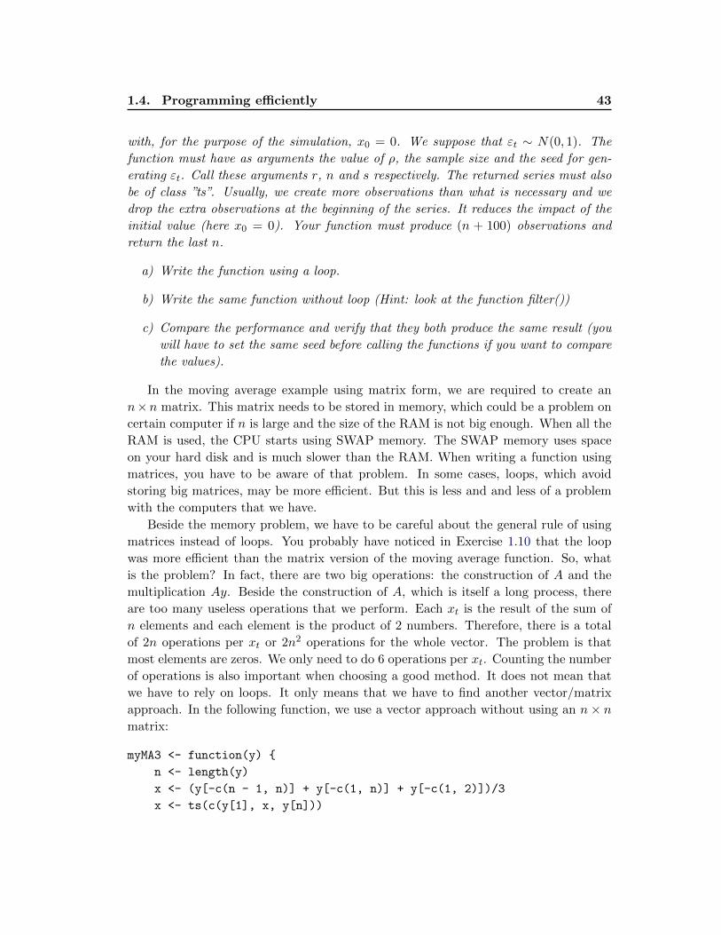
approach. In the following function, we use a vector approach without using an n× nmatrix:
myMA3 <- function(y) {
n <- length(y)
x <- (y[-c(n - 1, n)] + y[-c(1, n)] + y[-c(1, 2)])/3
x <- ts(c(y[1], x, y[n]))
44 Chapter 1. Introduction to R
attr(x, "tsp") <- attr(y, "tsp")
return(x)
}
> system.time(myMA3(y))
user system elapsed
0.000 0.000 0.001
It is even faster then myMA2(). We therefore modify the general rule to
Suggested Rule 1. Avoid loops if possible and replace them with vector of matrix
operations that minimize the number of operations. Constructing big matrices should
also be avoided.
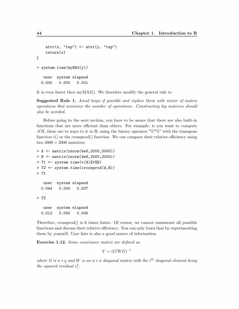
Before going to the next section, you have to be aware that there are also built-in
functions that are more efficient than others. For example, is you want to compute
A′B, there are to ways to it in R: using the binary operator ”%*%” with the transpose
function t() or the crossprod() function. We can compare their relative efficiency using
two 2000× 2000 matrices:
> A <- matrix(rnorm(4e6,2000,2000))
> B <- matrix(rnorm(4e6,2000,2000))
> T1 <- system.time(t(A)%*%B)
> T2 <- system.time(crossprod(A,B))
> T1
user system elapsed
0.044 0.000 0.037
> T2
user system elapsed
0.012 0.000 0.006
Therefore, crossprod() is 6 times faster. Of course, we cannot enumerate all possible
functions and discuss their relative efficiency. You can only learn that by experimenting
them by yourself. User lists is also a good source of information.
Exercise 1.12. Some covariance matrix are defined as
V = (G′WG)−1
where G is n×q and W is an n×n diagonal matrix with the ith diagonal element being
the squared residual ε2i .
1.4. Programming efficiently 45
a) Construct a function that computes the above operation with the argument of the
function being the matrix G and the vector of residuals e. In your function,
compute V exactly as it is written above.
b) Do the same, but without constructing the n× n matrix W .
c) Compare the relative efficiency of the two functions. To do so, generate a n × qmatrix G and n× 1 vector e randomly, with n = 5000 and q = 20.
1.4.2 Parallel programming
In this section, we briefly discuss some methods to improve efficiency by taking advan-
tage of the fact that computers are now equipped with multiple core processors. For
example, the Intel i7-2600 processor allows to send jobs to 8 cores simultaneously. If
you are lucky enough to work on a computer equipped with a Tesla GPU 2075 (graph-
ical processor unit), you can send up to 448 jobs simultaneously to your processor. It
is like having 448 computers working simultaneously. Parallel programing is a way of
write your program so that jobs are sent in blocks. For example, if you have 8 cores,
and want to run a simulation of 1000 iterations, you can run a loop of size equal to
125. In each loop, you send a block of 8 jobs to the 8 cores. These jobs are then run
simultaneously. You can then increase the speed of the simulation substantially.
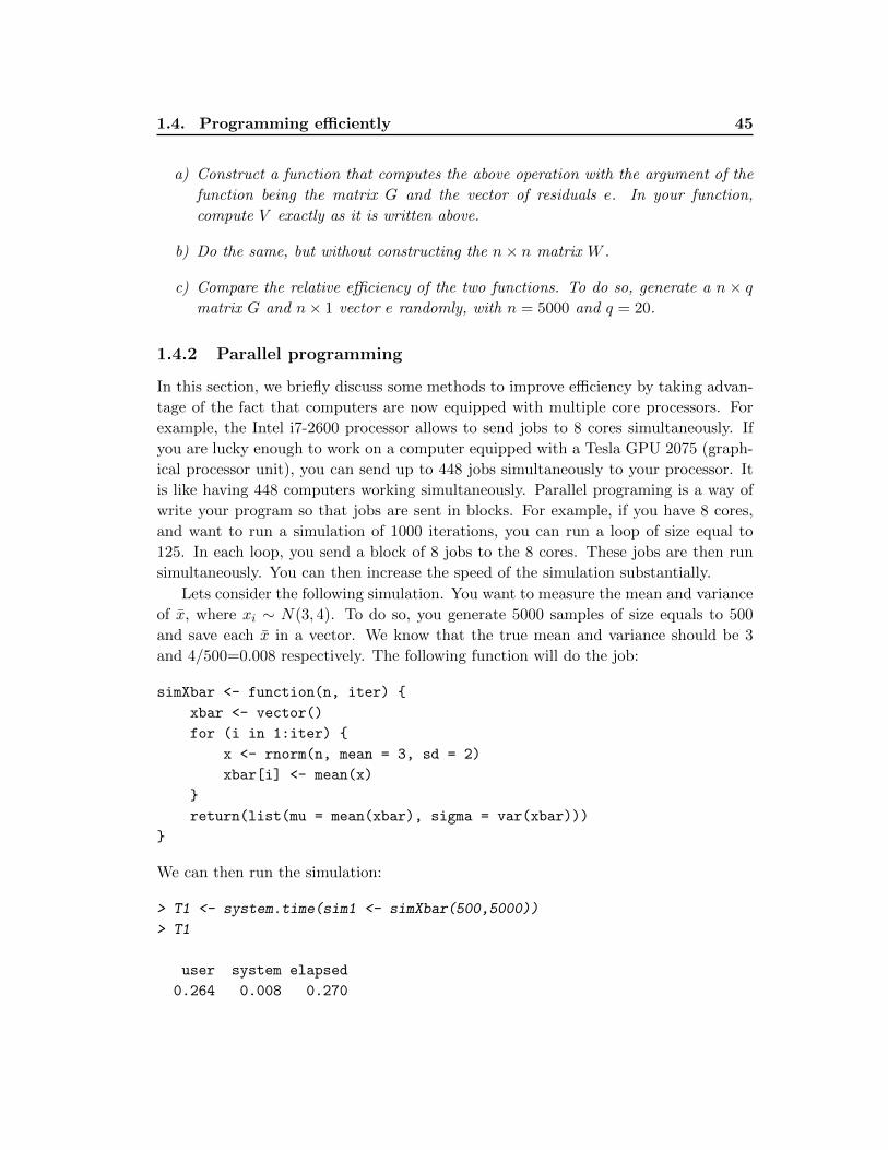
Lets consider the following simulation. You want to measure the mean and variance
of x, where xi ∼ N(3, 4). To do so, you generate 5000 samples of size equals to 500
and save each x in a vector. We know that the true mean and variance should be 3
and 4/500=0.008 respectively. The following function will do the job:
simXbar <- function(n, iter) {
xbar <- vector()
for (i in 1:iter) {
x <- rnorm(n, mean = 3, sd = 2)
xbar[i] <- mean(x)
}
return(list(mu = mean(xbar), sigma = var(xbar)))
}
We can then run the simulation:
> T1 <- system.time(sim1 <- simXbar(500,5000))
> T1
user system elapsed
0.264 0.008 0.270
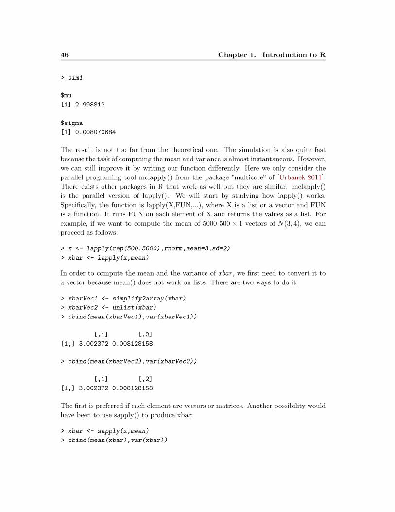
46 Chapter 1. Introduction to R
> sim1
$mu
[1] 2.998812
$sigma
[1] 0.008070684
The result is not too far from the theoretical one. The simulation is also quite fast
because the task of computing the mean and variance is almost instantaneous. However,
we can still improve it by writing our function differently. Here we only consider the
parallel programing tool mclapply() from the package ”multicore” of [Urbanek 2011].
There exists other packages in R that work as well but they are similar. mclapply()
is the parallel version of lapply(). We will start by studying how lapply() works.
Specifically, the function is lapply(X,FUN,...), where X is a list or a vector and FUN
is a function. It runs FUN on each element of X and returns the values as a list. For
example, if we want to compute the mean of 5000 500 × 1 vectors of N(3, 4), we can
proceed as follows:
> x <- lapply(rep(500,5000),rnorm,mean=3,sd=2)
> xbar <- lapply(x,mean)
In order to compute the mean and the variance of xbar, we first need to convert it to
a vector because mean() does not work on lists. There are two ways to do it:
> xbarVec1 <- simplify2array(xbar)
> xbarVec2 <- unlist(xbar)
> cbind(mean(xbarVec1),var(xbarVec1))
[,1] [,2]
[1,] 3.002372 0.008128158
> cbind(mean(xbarVec2),var(xbarVec2))
[,1] [,2]
[1,] 3.002372 0.008128158
The first is preferred if each element are vectors or matrices. Another possibility would
have been to use sapply() to produce xbar:
> xbar <- sapply(x,mean)
> cbind(mean(xbar),var(xbar))
1.4. Programming efficiently 47
[,1] [,2]
[1,] 3.002372 0.008128158
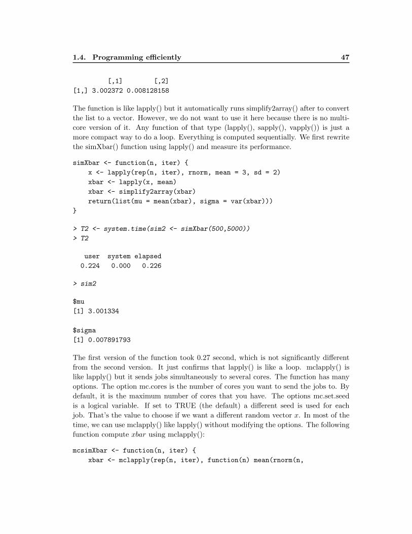
The function is like lapply() but it automatically runs simplify2array() after to convert
the list to a vector. However, we do not want to use it here because there is no multi-
core version of it. Any function of that type (lapply(), sapply(), vapply()) is just a
more compact way to do a loop. Everything is computed sequentially. We first rewrite
the simXbar() function using lapply() and measure its performance.
simXbar <- function(n, iter) {
x <- lapply(rep(n, iter), rnorm, mean = 3, sd = 2)
xbar <- lapply(x, mean)
xbar <- simplify2array(xbar)
return(list(mu = mean(xbar), sigma = var(xbar)))
}
> T2 <- system.time(sim2 <- simXbar(500,5000))
> T2
user system elapsed
0.224 0.000 0.226
> sim2
$mu
[1] 3.001334
$sigma
[1] 0.007891793
The first version of the function took 0.27 second, which is not significantly different
from the second version. It just confirms that lapply() is like a loop. mclapply() is
like lapply() but it sends jobs simultaneously to several cores. The function has many
options. The option mc.cores is the number of cores you want to send the jobs to. By
default, it is the maximum number of cores that you have. The options mc.set.seed
is a logical variable. If set to TRUE (the default) a different seed is used for each
job. That’s the value to choose if we want a different random vector x. In most of the
time, we can use mclapply() like lapply() without modifying the options. The following
function compute xbar using mclapply():
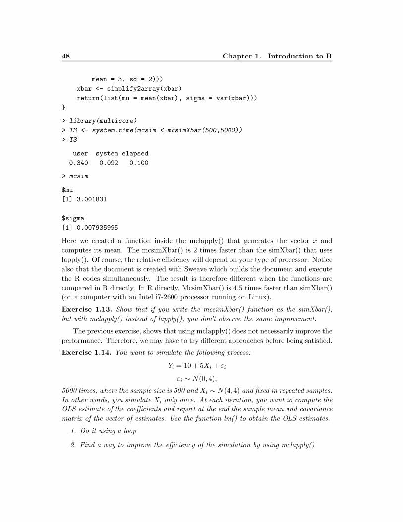
mcsimXbar <- function(n, iter) {
xbar <- mclapply(rep(n, iter), function(n) mean(rnorm(n,
48 Chapter 1. Introduction to R
mean = 3, sd = 2)))
xbar <- simplify2array(xbar)
return(list(mu = mean(xbar), sigma = var(xbar)))
}
> library(multicore)
> T3 <- system.time(mcsim <-mcsimXbar(500,5000))
> T3
user system elapsed
0.340 0.092 0.100
> mcsim
$mu
[1] 3.001831
$sigma
[1] 0.007935995
Here we created a function inside the mclapply() that generates the vector x and
computes its mean. The mcsimXbar() is 2 times faster than the simXbar() that uses
lapply(). Of course, the relative efficiency will depend on your type of processor. Notice
also that the document is created with Sweave which builds the document and execute
the R codes simultaneously. The result is therefore different when the functions are
compared in R directly. In R directly, McsimXbar() is 4.5 times faster than simXbar()
(on a computer with an Intel i7-2600 processor running on Linux).
Exercise 1.13. Show that if you write the mcsimXbar() function as the simXbar(),
but with mclapply() instead of lapply(), you don’t observe the same improvement.
The previous exercise, shows that using mclapply() does not necessarily improve the
performance. Therefore, we may have to try different approaches before being satisfied.
Exercise 1.14. You want to simulate the following process:
Yi = 10 + 5Xi + εi
εi ∼ N(0, 4),
5000 times, where the sample size is 500 and Xi ∼ N(4, 4) and fixed in repeated samples.
In other words, you simulate Xi only once. At each iteration, you want to compute the
OLS estimate of the coefficients and report at the end the sample mean and covariance
matrix of the vector of estimates. Use the function lm() to obtain the OLS estimates.
1. Do it using a loop
2. Find a way to improve the efficiency of the simulation by using mclapply()
Chapter 2
Floating points arithmetic
Contents
2.1 What is a floating-point number . . . . . . . . . . . . . . . . . . 49
2.2 Rounding errors . . . . . . . . . . . . . . . . . . . . . . . . . . . . 54
This Chapter is only an introduction to floating-points arithmetic. The
goal is only to make you realize that most numbers that we use in our
numerical projects are only approximations. Our results are therefore sub-
ject to rounding errors that may accumulate if we are not careful. If
you want a complete and detailed presentation of floating-point numbers, see
[Goldberg 1991](http://neo.dmcs.p.lodz.pl/ak/IEEE754 article.pdf). As an example,
the number 0.1 cannot be represented exactly by computers. We will see why in next
section. We can verify that by the following small experiment:
> .1+.1+.1==.3
[1] FALSE
R tells us that 0.1+0.1+0.1 is not equal to 0.3. However, the difference is small as we
can see:
> (.1+.1+.1)-.3
[1] 5.551115e-17
However, when we have to deal with thousands of operations, the error may become
more substantial. In the next section, we explain briefly how a computer store numbers
and why it cannot represent exactly simple numbers such as 0.1.
2.1 What is a floating-point number
A floating-point number is a real number that can be represented exactly by a computer.
First, computers store information in binary format (0’s and 1’s). In order to have
50 Chapter 2. Floating points arithmetic
software that are portable from one computer or operating system to another, we need
a stable way or dealing with floating-point numbers. Different results obtain on different
computers is enough to make a program crash. The most common standard used in
computers is the IEEE 754 (Institute of Electrical and Electronics Engineers). It is
a binary standard which means that numbers are represented in base 2. One of the
reasons for using the base 2 is related to the tightness of the relative error that comes
from the approximation of real numbers by floating-point numbers. Unless we want
to build computers, we don’t need to know more about the advantage of using that
standard. In binary format, integers are exactly represented by computers:
1 = 1(20) =2 1
2 = 1(21) + 0(20) =2 10
3 = 1(21) + 1(20) =2 11
4 = 1(22) + 0(21) + 0(20) =2 100
... =2...
N =
p∑i=0
di(2i) =2 dpdp−1 · · · d0
where =2 means ”equals in base 2” and di’s are either 0 or 1. Of course, the number of
bits restricts the number of integers that can be exactly represented. In general, a real
floating-point number, x, is represented as follows:
x = ±[d0 + d1(2
−1) + d2(2−2) + · · ·+ dp−1(2
−(p−1))]
2e,
or simply
x = ± [d0.d1d2 · · · dp−1]2 2e,
where []2 means that the inside of the brackets is expressed in base 2, p is called the
precision (or the number of digits) and e the exponent. The term d0.d1...dp−1 is called
the significant. For example:
4.5 = 22 + 2−1 = (1 + 2−3)22 = [1.001]2 × 22,
which implies that d0 = 1, d3 = 1 (or a significant equals to 1.001), e = 2 (or 10 in
base 2) and all other di are equal to zero. Of course there are more than one ways to
represent 4.5. Here is another one:
4.5 = (2−1 + 2−4)23,
which implies d1 = d4 = 1, e = 3 and all other di’s equal to zero. However, the
number is uniquely represented if we impose the normalization d0 = 1. Furthermore,
2.1. What is a floating-point number 51
the normalization saves us a bit because there is no need to store d0 since it is always
1. The bits are allocated between the storage of the exponent, the (p− 1) di’s and the
sign (e.g. 1 if + and 0 if -). The exponent is store as an unsigned integer, which implies
that the number of different exponents is (emax− emin). Therefore, the number of bits
required to store a floating-point number is approximately:
Bits = log2 (emax − emin) + (p− 1) + 1
In R the allocation is stored in the variable .Machine:
> print(p <- .Machine$double.digits)
[1] 53
> print(emax <- .Machine$double.max.exp)
[1] 1024
> print(emin <- .Machine$double.min.exp)
[1] -1022
> bits <- log(emax-emin,2)+(p-1)+1
> bits
[1] 63.99859
It gives 1 bit for the sign, 11 for the exponent and 52 for the significant. In fact,
R follows the IEEE-754 standard for double precision floating-point numbers. Other
important numbers are stored in .Machine. The first is the machine-epsilon (ε). It is
usually defined as β−p+1/2, where β is the base. It is the smallest positive floating-point
number, x, such that (1 + x) 6= 1:
> print(eps<-.Machine$double.eps)
[1] 2.220446e-16
> 1+eps==1
[1] FALSE
It is not the smallest number, which is rather equal to 2emin , but the highest relative
error that comes from approximating a real numbers by its nearest floating-point num-
ber. The accuracy of algorithms is often measured in terms of the machine-epsilon.
52 Chapter 2. Floating points arithmetic
A bad algorithms may produce errors of size nε with n >> 1. We therefore want to
choose algorithms that minimizes n. In the example we showed at the beginning of
the chapter, R returned FALSE to the question: 0.1 + 0.1 + 0.1 = 0.3? But, since
0.1 does not have an exact floating-point representation there is a rounding error that
accumulates when summing them. If we want to compare the numbers we need to take
into account these rounding errors. The function all.equal() compares numbers with a
certain level of tolerance. So, they don’t necessarily have to be exactly equal. If we go
back to are first example:
> .1+.1+.1==.3
[1] FALSE
> all.equal(.1+.1+.1,.3,tolerance=eps)
[1] TRUE
The interpretation of the above result is that (.1+.1+.1) 6= 0.3 only because of rounding
errors. The maximum and minimum floating-point numbers are:
> .Machine$double.xmax
[1] 1.797693e+308
> .Machine$double.xmin
[1] 2.225074e-308
Anything above the xmax is considered to be equal to infinity an anything below xmin
is considered to be equal to 0:
> .Machine$double.xmax*2
[1] Inf
We conclude this section by looking at another important ”number” that may appears
when performing some operations. The ”number” is NA or NaN, which means ”Not
a Number”. It will result from operations that produced indeterminate results. It is
not to be confused with operations that produce infinity. For example, 1/0 = ∞ but
0/0 = NA:
> 1/0
[1] Inf

2.1. What is a floating-point number 53
> 0/0
[1] NaN
Here are other examples:
> Inf-Inf
[1] NaN
> log(-2)
[1] NaN
> sqrt(-1)
[1] NaN
> Inf/Inf
[1] NaN
Of course, we cannot compare NA numbers. NA, as it is called, is not a number.
Therefore, we cannot use the logical operator ”==” to verify if an operation produces
an NA. In fact the result will also be an NA. There is a function in R that verify that:
> (0/0) == NA
[1] NA
> is.na(0/0)
[1] TRUE
However, we can use logical operators with infinity:
> (1/0)==Inf
[1] TRUE
> 1e400==Inf
[1] TRUE
> 1e200<Inf
[1] TRUE
54 Chapter 2. Floating points arithmetic
2.2 Rounding errors
This section briefly covers the issue of rounding errors created by numerical compu-
tations. Again, we cannot cover it in details. In fact, it may be quite complicated to
measure rounding errors from certain algorithms. But knowing how they are created
may help us developing good programming habits. It will also help justifying some
methods that will be presented in the next chapters.
In order to illustrate the problem related to rounding errors, consider the case of
floating-point numbers represented in base 10 with the number of digits p equals to 3
(remember that the number of digits after the point is equal to (p− 1)). In that case,
π is approximated by the floating-point number 3.14 × 100. Suppose the true value
is 3.1416. The term ”last place” refers to the last decimal given by the floating-point
representation (or 10−p+1). The error is 0.0016 = 0.16× 10⁻² or 0.16ulps (units of the
last place). An error smaller than 1ulps means that the last digit is not contaminated.
Error from approximating a real number is always less than 1ulps. However, we often
get errors greater than 1ulps when results come from mathematical operations. As an
example, suppose the result of a computation is 3.12 × 100 and that the true answer
is 3.14 × 100. The error is then equal to 2ulps. In the IEEE standard, where p = 53,
the precision is up to about the 16th decimal (the 53th digit in base 2 refers to the 16th
digit in base 10).
The error measure in ulps is affected by multiplications. Consider the approximated
π above. Since it is represented by 3.14 × 100, if we multiply it by 2, the result
will become 6.28 × 100. The true value is 2π = 6.2832 which implies an error of
0.32ulps. Another measure of rounding error is the relative error defined as the error
divided by the true value and it is often expressed in term of the machine-epsilon. The
relative error for π is 0.0016/3.1416 = 0.0005 and the one for the computation of 2π
is 0.0032/6.2832 = 0.0005. It is therefore unaffected by the operation. The relative
error in terms of the machine-epsilon is [error/(TRUE ∗ ε)]ε. In our example, the
machine-epsilon is 10−2/2 = 0.005. The relative error for π or 2π is therefore 0.1ε.
There is a link between the error and the number of contaminated digits. If the
error is n ulps the number of contaminated digits is logβ n, if the relative error is nε
the number of contaminated digits is logβ n. Suppose we want to compute (x − y).
Suppose also that the base is 10, p=3 and the computer only keeps 2 decimal when
performing operations. In the first case, y = 2.15 × 10¹² and x = 1, 25 × 10−5. The
computer rewrites the numbers using the same exponent and keep only 2 digits:
y − x = 2.15× 10¹² − 0.00× 1012 = 2.15× 10¹²
The error is very small and no digits are contaminated. Consider the second case for
which y = 10.1 and x = 9.93. Using the same rule, we obtain:
y − x = 1.01× 101 − 0.99× 101 = 2.00× 10⁻¹
2.2. Rounding errors 55
The error is 30ulps which implies a relative error of [0.03/(0.2 ∗ 0.005)]ε = 30ε.
log10 30 > 1 meaning that the two digits are contaminated. The error from the last
subtraction is called ”Catastrophic cancellation”, and it arises when x and y are very
close to each other. Of course, we would not have obtained the same error with double
precision floating-point numbers (p = 53 and β = 2). This example is meant to easily
show what happens when we subtract numbers of similar values. In reality, computers
are smarter than that. They usually have what we call ”Guard Digits” which are extra
digits used during floating-point operations. In our example, one Guard Digit would
have been enough to have no error. However, ”Catastrophic cancellation” exists even
in double precision systems. The error is small in absolute term but quite big if we
compare it with the error from other floating-point operations. To have an idea in
double precision computations, consider the following example:
> x <- 332.2234
> y <- 332.223395
> s <- x-y
> error <- s-0.000005
> error
[1] 4.421963e-14
The error is therefore approximately 442ulps (if we consider that p=53 corresponds to
the 16th decimals). However, what we just computed is not really the error coming from
(y − x). In fact, rounding errors is hard to measure with a computer because we are
not really subtracting the true solution (0.000005 does not have an exact floating-point
representation). Catastrophic cancellation occurs in fact when we subtract numbers
who are subject to rounding errors. In other words, numbers that come from floating-
point operations (ex. y2− x2). In that case, the rounding error is greater than the one
from approximating a real number. If the numbers are close, the subtraction eliminates
the good digits and we are left with the bad ones. Lets see what happens if y and x
are not close:
> x <- 2.57
> y <- 0.13
> s <- x-y
> error <- s-2.44
> error
[1] 0
We don’t really care in economics about an error at the 14th decimal. We don’t build
bridges. Therefore, we won’t worry when the number of floating-point operations is
56 Chapter 2. Floating points arithmetic
small. But, these small errors can become huge if the operations are repeated hundreds
or thousands of times. For example, when we work with big systems of matrices,
solving the system requires many sums, products, subtractions and divisions. If we
are not careful about how to minimize rounding errors, we may end up with a wrong
solution. Even if we do use some accurate algorithms, there exists iterative procedures
to reduce the rounding error further. We will cover that in the next section. Consider
only the operation to compute the OLS estimate:
β = (X ′X)−1X ′Y
Suppose the sample size is 1000 and the number of coefficients is 10. Then, we need to
compute 1000 sums and multiplications for each of the 100 elements of (X ′X) and each
of the 10 elements of (X ′Y ). But, that’s not the end. We now have to invert (X ′X)
(we don’t really do that, as we’ll see in the next chapter) and multiply the inverse by
(X’Y). Fortunately, there exists a method that is less sensitive to rounding errors. We
don’t even have to compute X ′X. We’ll cover that in the next chapter.
The problem with floating-point arithmetic is that a method can be accurate most
of the time but very bad in some cases, when our variables take some particular values.
And because there is no error message that appears, we think that everything is fine.
The purpose of this chapter is only to make sure that you are aware of that. It will
also justify many numerical approaches that we will cover throughout the course.
We conclude this chapter with two examples. Suppose we want to compute the
sum of the element of a vector. If the elements of the vector come from floating-point
operations, the usual sum,∑n
i=1 xi, could produce large rounding errors. It would
be even worse if some successive xi’s were close to each other in absolute value with
different signs, because we would face multiple catastrophic cancellations. The first
solution is to order the vector and to sum the element from the smallest to the largest.
Adding a small number to a large number may make us loose the last digits of the
small one. That’s why sorting may improve the accuracy of the sum. The second is to
use the following algorithm:
Exercise 2.1. Write the R function mySum(x) of the Algorithm 2.1. Create a
100, 000 × 1 vector with each element equals to 0.1. Compare the accuracy of your
function with the R function sum().
Algorithm 2.1 may seem to be an obscure way to improve accuracy. It is in fact
quite hard to come up with such algorithms. Another way to minimize rounding errors
is to minimize the number of operations when it is necessary. since it reduces the
accumulation of errors. In fact, it kills two birds with the same stone because it also
makes the algorithm faster. Suppose for example that we want to compute the following
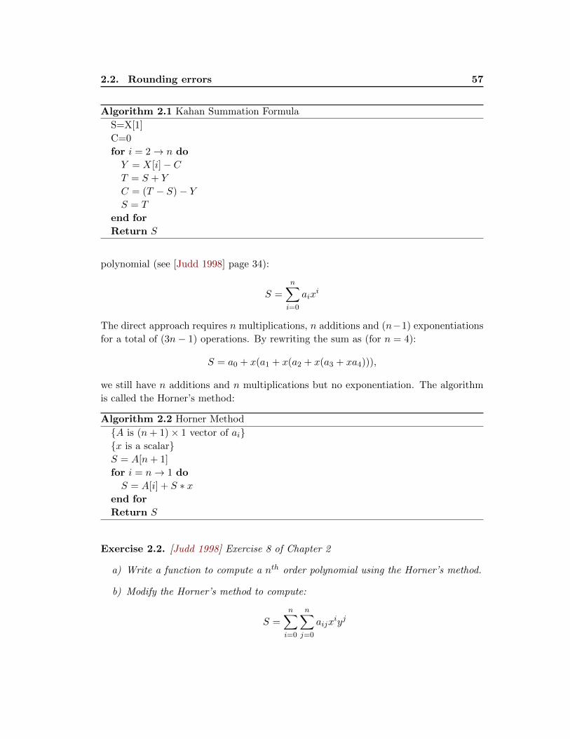
2.2. Rounding errors 57
Algorithm 2.1 Kahan Summation Formula
S=X[1]
C=0
for i = 2→ n do
Y = X[i]− CT = S + Y
C = (T − S)− YS = T
end for
Return S
polynomial (see [Judd 1998] page 34):
S =
n∑i=0
aixi
The direct approach requires n multiplications, n additions and (n−1) exponentiations
for a total of (3n− 1) operations. By rewriting the sum as (for n = 4):
S = a0 + x(a1 + x(a2 + x(a3 + xa4))),
we still have n additions and n multiplications but no exponentiation. The algorithm
is called the Horner’s method:
Algorithm 2.2 Horner Method
{A is (n+ 1)× 1 vector of ai}{x is a scalar}S = A[n+ 1]
for i = n→ 1 do
S = A[i] + S ∗ xend for
Return S
Exercise 2.2. [Judd 1998] Exercise 8 of Chapter 2
a) Write a function to compute a nth order polynomial using the Horner’s method.
b) Modify the Horner’s method to compute:
S =n∑i=0
n∑j=0
aijxiyj

58 Chapter 2. Floating points arithmetic
c) Modify the Horner’s method to compute:
S =n∑i=0
n∑j=0
n∑l=0
aijlxiyjzl
Chapter 3
Linear Equations and Iterative
Methods
Contents
3.1 Linear algebra . . . . . . . . . . . . . . . . . . . . . . . . . . . . . 59
3.2 Iterative method . . . . . . . . . . . . . . . . . . . . . . . . . . . . 66
3.2.1 Stopping rules . . . . . . . . . . . . . . . . . . . . . . . . . . . . . 66
3.2.2 Fixed-Point Iteration . . . . . . . . . . . . . . . . . . . . . . . . . . 70
3.2.3 Gauss-Jacobi and Gauss-Seidel . . . . . . . . . . . . . . . . . . . . 71
3.2.4 Acceleration and Stabilization Methods . . . . . . . . . . . . . . . 78
3.1 Linear algebra
Suppose we want to compute the following problem:
Ax = y
The way we learn how to solve this system in basic textbooks is by inverting A and
multiplying y by the inverse. In other words, the solution is:
x = A−1y
This solution is right mathematically ans has a nice analytical form, but is not rec-
ommended numerically. Suppose you want to compute the inverse using textbook
definition. The number of operations to compute the determinant for an n× n matrix
is O(n!). We want to minimize the number of operations and also the number of catas-
trophic cancellations. The LU decomposition with pivoting is an algorithm developed
for that purpose. Pivoting is done to avoid unstable operations and LU decomposition
to reduce the number of operations. Consider the following case:
> A <- matrix(c(5,4,7,8,6,3,2,9,1),3,3)
> y <- c(2,4,6)
> A
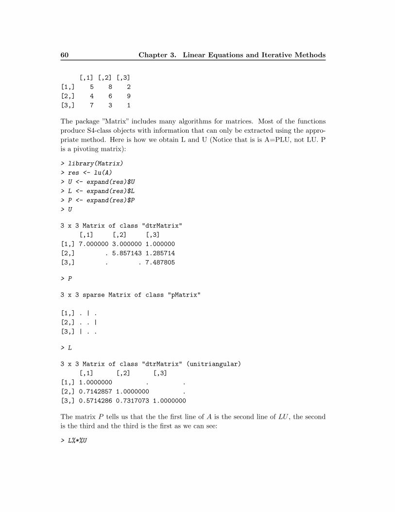
60 Chapter 3. Linear Equations and Iterative Methods
[,1] [,2] [,3]
[1,] 5 8 2
[2,] 4 6 9
[3,] 7 3 1
The package ”Matrix” includes many algorithms for matrices. Most of the functions
produce S4-class objects with information that can only be extracted using the appro-
priate method. Here is how we obtain L and U (Notice that is is A=PLU, not LU. P
is a pivoting matrix):
> library(Matrix)
> res <- lu(A)
> U <- expand(res)$U
> L <- expand(res)$L
> P <- expand(res)$P
> U
3 x 3 Matrix of class "dtrMatrix"
[,1] [,2] [,3]
[1,] 7.000000 3.000000 1.000000
[2,] . 5.857143 1.285714
[3,] . . 7.487805
> P
3 x 3 sparse Matrix of class "pMatrix"
[1,] . | .
[2,] . . |
[3,] | . .
> L
3 x 3 Matrix of class "dtrMatrix" (unitriangular)
[,1] [,2] [,3]
[1,] 1.0000000 . .
[2,] 0.7142857 1.0000000 .
[3,] 0.5714286 0.7317073 1.0000000
The matrix P tells us that the the first line of A is the second line of LU , the second
is the third and the third is the first as we can see:
> L%*%U
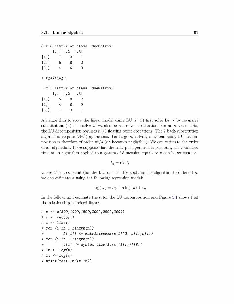
3.1. Linear algebra 61
3 x 3 Matrix of class "dgeMatrix"
[,1] [,2] [,3]
[1,] 7 3 1
[2,] 5 8 2
[3,] 4 6 9
> P%*%L%*%U
3 x 3 Matrix of class "dgeMatrix"
[,1] [,2] [,3]
[1,] 5 8 2
[2,] 4 6 9
[3,] 7 3 1
An algorithm to solve the linear model using LU is: (i) first solve Lz=y by recursive
substitution, (ii) then solve Ux=z also be recursive substitution. For an n× n matrix,
the LU decomposition requires n3/3 floating point operations. The 2 back-substitution
algorithms require O(n2) operations. For large n, solving a system using LU decom-
position is therefore of order n3/3 (n2 becomes negligible). We can estimate the order
of an algorithm. If we suppose that the time per operation is constant, the estimated
time of an algorithm applied to a system of dimension equals to n can be written as:
tn = Cnα,
where C is a constant (for the LU, α = 3). By applying the algorithm to different n,
we can estimate α using the following regression model:
log (tn) = α0 + α log (n) + εn
In the following, I estimate the α for the LU decomposition and Figure 3.1 shows that
the relationship is indeed linear.
> n <- c(500,1000,1500,2000,2500,3000)
> t <- vector()
> A <- list()
> for (i in 1:length(n))
+ A[[i]] <- matrix(rnorm(n[i]^2),n[i],n[i])
> for (i in 1:length(n))
+ t[i] <- system.time(lu(A[[i]]))[[3]]
> ln <- log(n)
> lt <- log(t)
> print(res<-lm(lt~ln))
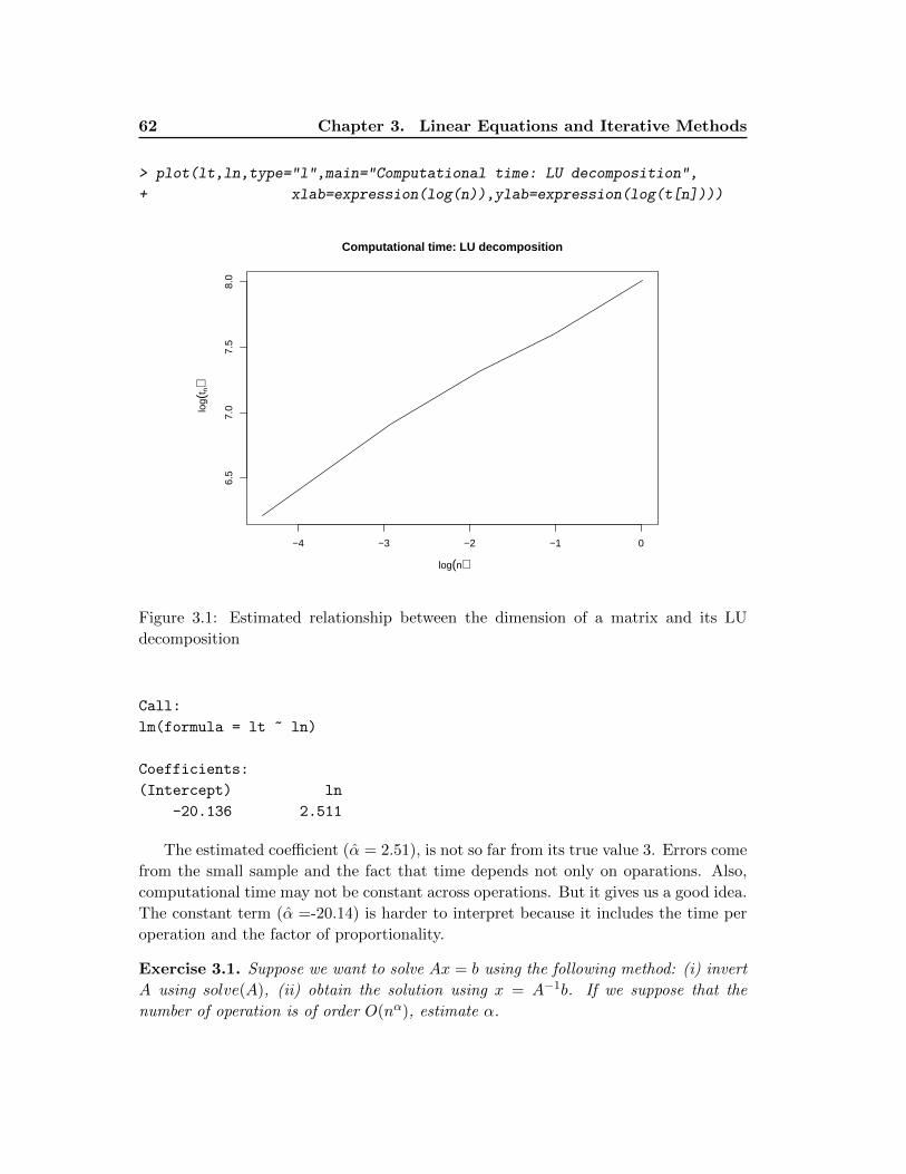
62 Chapter 3. Linear Equations and Iterative Methods
> plot(lt,ln,type="l",main="Computational time: LU decomposition",
+ xlab=expression(log(n)),ylab=expression(log(t[n])))
−4 −3 −2 −1 0
6.5
7.0
7.5
8.0
Computational time: LU decomposition
log(n)
log(
t n)
Figure 3.1: Estimated relationship between the dimension of a matrix and its LU
decomposition
Call:
lm(formula = lt ~ ln)
Coefficients:
(Intercept) ln
-20.136 2.511
The estimated coefficient (α = 2.51), is not so far from its true value 3. Errors come
from the small sample and the fact that time depends not only on oparations. Also,
computational time may not be constant across operations. But it gives us a good idea.
The constant term (α =-20.14) is harder to interpret because it includes the time per
operation and the factor of proportionality.
Exercise 3.1. Suppose we want to solve Ax = b using the following method: (i) invert
A using solve(A), (ii) obtain the solution using x = A−1b. If we suppose that the
number of operation is of order O(nα), estimate α.
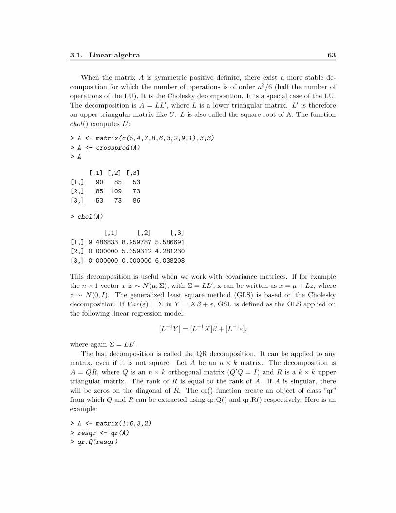
3.1. Linear algebra 63
When the matrix A is symmetric positive definite, there exist a more stable de-
composition for which the number of operations is of order n3/6 (half the number of
operations of the LU). It is the Cholesky decomposition. It is a special case of the LU.
The decomposition is A = LL′, where L is a lower triangular matrix. L′ is therefore
an upper triangular matrix like U . L is also called the square root of A. The function
chol() computes L′:
> A <- matrix(c(5,4,7,8,6,3,2,9,1),3,3)
> A <- crossprod(A)
> A
[,1] [,2] [,3]
[1,] 90 85 53
[2,] 85 109 73
[3,] 53 73 86
> chol(A)
[,1] [,2] [,3]
[1,] 9.486833 8.959787 5.586691
[2,] 0.000000 5.359312 4.281230
[3,] 0.000000 0.000000 6.038208
This decomposition is useful when we work with covariance matrices. If for example
the n× 1 vector x is ∼ N(µ,Σ), with Σ = LL′, x can be written as x = µ+Lz, where
z ∼ N(0, I). The generalized least square method (GLS) is based on the Cholesky
decomposition: If V ar(ε) = Σ in Y = Xβ + ε, GSL is defined as the OLS applied on
the following linear regression model:
[L−1Y ] = [L−1X]β + [L−1ε],
where again Σ = LL′.
The last decomposition is called the QR decomposition. It can be applied to any
matrix, even if it is not square. Let A be an n × k matrix. The decomposition is
A = QR, where Q is an n × k orthogonal matrix (Q′Q = I) and R is a k × k upper
triangular matrix. The rank of R is equal to the rank of A. If A is singular, there
will be zeros on the diagonal of R. The qr() function create an object of class ”qr”
from which Q and R can be extracted using qr.Q() and qr.R() respectively. Here is an
example:
> A <- matrix(1:6,3,2)
> resqr <- qr(A)
> qr.Q(resqr)
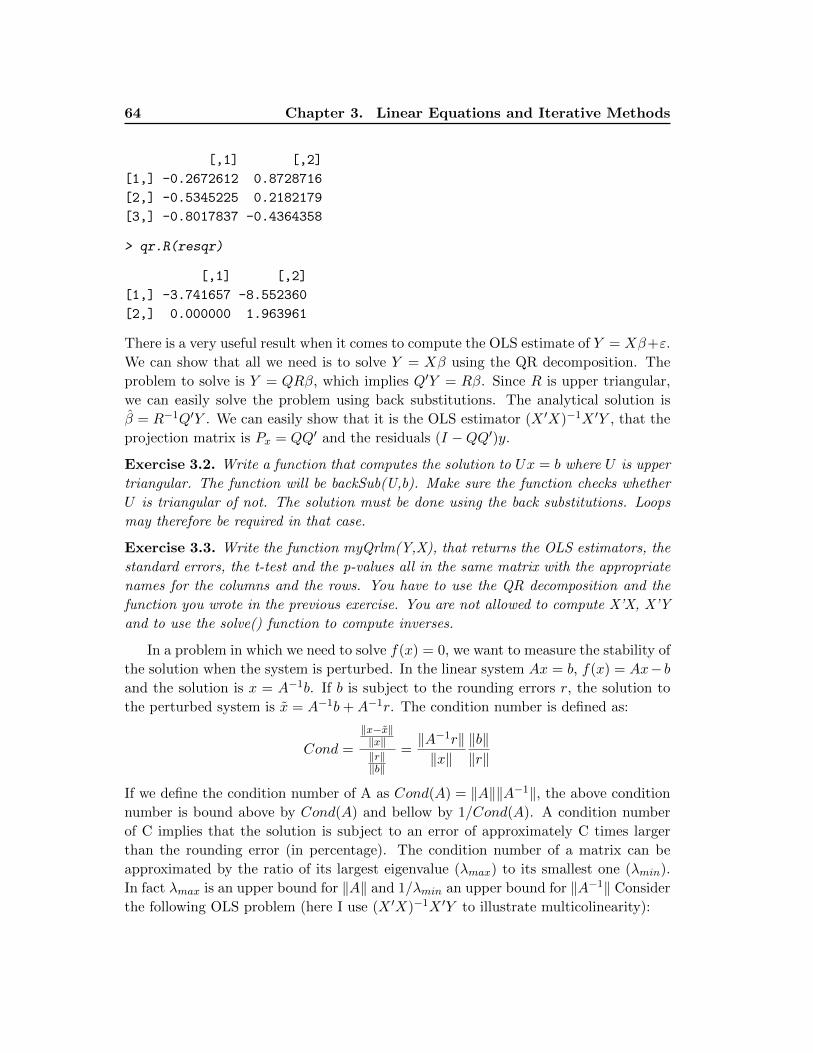
64 Chapter 3. Linear Equations and Iterative Methods
[,1] [,2]
[1,] -0.2672612 0.8728716
[2,] -0.5345225 0.2182179
[3,] -0.8017837 -0.4364358
> qr.R(resqr)
[,1] [,2]
[1,] -3.741657 -8.552360
[2,] 0.000000 1.963961
There is a very useful result when it comes to compute the OLS estimate of Y = Xβ+ε.
We can show that all we need is to solve Y = Xβ using the QR decomposition. The
problem to solve is Y = QRβ, which implies Q′Y = Rβ. Since R is upper triangular,
we can easily solve the problem using back substitutions. The analytical solution is
β = R−1Q′Y . We can easily show that it is the OLS estimator (X ′X)−1X ′Y , that the
projection matrix is Px = QQ′ and the residuals (I −QQ′)y.
Exercise 3.2. Write a function that computes the solution to Ux = b where U is upper
triangular. The function will be backSub(U,b). Make sure the function checks whether
U is triangular of not. The solution must be done using the back substitutions. Loops
may therefore be required in that case.
Exercise 3.3. Write the function myQrlm(Y,X), that returns the OLS estimators, the
standard errors, the t-test and the p-values all in the same matrix with the appropriate
names for the columns and the rows. You have to use the QR decomposition and the
function you wrote in the previous exercise. You are not allowed to compute X’X, X’Y
and to use the solve() function to compute inverses.
In a problem in which we need to solve f(x) = 0, we want to measure the stability of
the solution when the system is perturbed. In the linear system Ax = b, f(x) = Ax− band the solution is x = A−1b. If b is subject to the rounding errors r, the solution to
the perturbed system is x = A−1b+A−1r. The condition number is defined as:
Cond =
‖x−x‖‖x‖‖r‖‖b‖
=‖A−1r‖‖x‖
‖b‖‖r‖
If we define the condition number of A as Cond(A) = ‖A‖‖A−1‖, the above condition
number is bound above by Cond(A) and bellow by 1/Cond(A). A condition number
of C implies that the solution is subject to an error of approximately C times larger
than the rounding error (in percentage). The condition number of a matrix can be
approximated by the ratio of its largest eigenvalue (λmax) to its smallest one (λmin).
In fact λmax is an upper bound for ‖A‖ and 1/λmin an upper bound for ‖A−1‖ Consider
the following OLS problem (here I use (X ′X)−1X ′Y to illustrate multicolinearity):
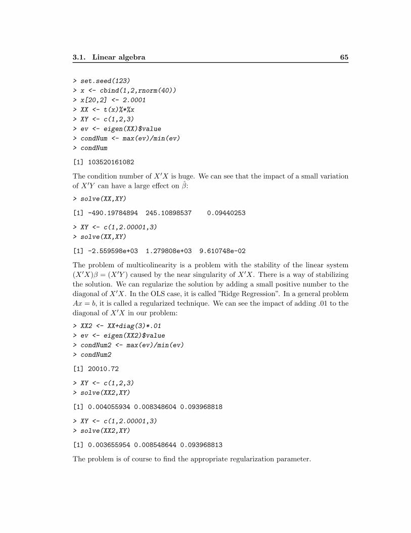
3.1. Linear algebra 65
> set.seed(123)
> x <- cbind(1,2,rnorm(40))
> x[20,2] <- 2.0001
> XX <- t(x)%*%x
> XY <- c(1,2,3)
> ev <- eigen(XX)$value
> condNum <- max(ev)/min(ev)
> condNum
[1] 103520161082
The condition number of X ′X is huge. We can see that the impact of a small variation
of X ′Y can have a large effect on β:
> solve(XX,XY)
[1] -490.19784894 245.10898537 0.09440253
> XY <- c(1,2.00001,3)
> solve(XX,XY)
[1] -2.559598e+03 1.279808e+03 9.610748e-02
The problem of multicolinearity is a problem with the stability of the linear system
(X ′X)β = (X ′Y ) caused by the near singularity of X ′X. There is a way of stabilizing
the solution. We can regularize the solution by adding a small positive number to the
diagonal of X ′X. In the OLS case, it is called ”Ridge Regression”. In a general problem
Ax = b, it is called a regularized technique. We can see the impact of adding .01 to the
diagonal of X ′X in our problem:
> XX2 <- XX+diag(3)*.01
> ev <- eigen(XX2)$value
> condNum2 <- max(ev)/min(ev)
> condNum2
[1] 20010.72
> XY <- c(1,2,3)
> solve(XX2,XY)
[1] 0.004055934 0.008348604 0.093968818
> XY <- c(1,2.00001,3)
> solve(XX2,XY)
[1] 0.003655954 0.008548644 0.093968813
The problem is of course to find the appropriate regularization parameter.
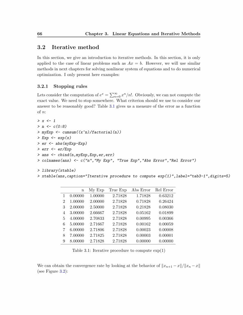
66 Chapter 3. Linear Equations and Iterative Methods
3.2 Iterative method
In this section, we give an introduction to iterative methods. In this section, it is only
applied to the case of linear problems such as Ax = b. However, we will use similar
methods in next chapters for solving nonlinear system of equations and to do numerical
optimization. I only present here examples:
3.2.1 Stopping rules
Lets consider the computation of ex =∑∞
n=0 xn/n!. Obviously, we can not compute the
exact value. We need to stop somewhere. What criterion should we use to consider our
answer to be reasonably good? Table 3.1 gives us a measure of the error as a function
of n:
> x <- 1
> n <- c(0:8)
> myExp <- cumsum((x^n)/factorial(n))
> Exp <- exp(x)
> er <- abs(myExp-Exp)
> err <- er/Exp
> ans <- cbind(n,myExp,Exp,er,err)
> colnames(ans) <- c("n","My Exp", "True Exp","Abs Error","Rel Error")
> library(xtable)
> xtable(ans,caption="Iterative procedure to compute exp(1)",label="tab3-1",digits=5)
n My Exp True Exp Abs Error Rel Error
1 0.00000 1.00000 2.71828 1.71828 0.63212
2 1.00000 2.00000 2.71828 0.71828 0.26424
3 2.00000 2.50000 2.71828 0.21828 0.08030
4 3.00000 2.66667 2.71828 0.05162 0.01899
5 4.00000 2.70833 2.71828 0.00995 0.00366
6 5.00000 2.71667 2.71828 0.00162 0.00059
7 6.00000 2.71806 2.71828 0.00023 0.00008
8 7.00000 2.71825 2.71828 0.00003 0.00001
9 8.00000 2.71828 2.71828 0.00000 0.00000
Table 3.1: Iterative procedure to compute exp(1)
We can obtain the convergence rate by looking at the behavior of ‖xn+1−x‖/‖xn−x‖(see Figure 3.2):
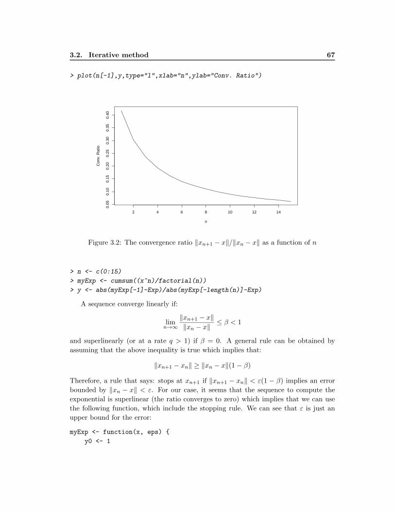
3.2. Iterative method 67
> plot(n[-1],y,type="l",xlab="n",ylab="Conv. Ratio")
2 4 6 8 10 12 14
0.05
0.10
0.15
0.20
0.25
0.30
0.35
0.40
n
Con
v. R
atio
Figure 3.2: The convergence ratio ‖xn+1 − x‖/‖xn − x‖ as a function of n
> n <- c(0:15)
> myExp <- cumsum((x^n)/factorial(n))
> y <- abs(myExp[-1]-Exp)/abs(myExp[-length(n)]-Exp)
A sequence converge linearly if:
limn→∞
‖xn+1 − x‖‖xn − x‖
≤ β < 1
and superlinearly (or at a rate q > 1) if β = 0. A general rule can be obtained by
assuming that the above inequality is true which implies that:
‖xn+1 − xn‖ ≥ ‖xn − x‖(1− β)
Therefore, a rule that says: stops at xn+1 if ‖xn+1 − xn‖ < ε(1 − β) implies an error
bounded by ‖xn − x‖ < ε. For our case, it seems that the sequence to compute the
exponential is superlinear (the ratio converges to zero) which implies that we can use
the following function, which include the stopping rule. We can see that ε is just an
upper bound for the error:
myExp <- function(x, eps) {
y0 <- 1
68 Chapter 3. Linear Equations and Iterative Methods
n <- 1
crit <- 1000
while (crit > eps) {
y <- y0 + (x^n)/factorial(n)
crit <- abs(y - y0)
n <- n + 1
y0 <- y
}
return(y)
}
> abs(myExp(2,1e-3)-exp(2))
[1] 6.138994e-05
> abs(myExp(2,1e-8)-exp(2))
[1] 4.142358e-10
> abs(myExp(2,1e-12)-exp(2))
[1] 4.618528e-14
Sometimes we also see rules based on the relative variation of the xn. This rule is:
stop at xn+1 if ‖xn+1 − xn‖/(1 + ‖xn‖) ≤ ε. The value in the denominator is to allow
convergence to zero. This rule however does not work well with sequences that converge
linearly. We can see that using the sequence xn =∑n
i=1(1/i):
> N <- 100
> n <- 1:N
> x <- sum(1/n)
> xn <- cumsum(1/n[-N])
> y <- abs(xn[-1]-x)/abs(xn[-length(xn)]-x)
> beta <- max(y)
> beta
[1] 0.973315
In Figure 3.3 we can see that β as an upper bound around 1, which shows that
there is no convergence. Using the first rule we would never conclude that the sequence
converges.
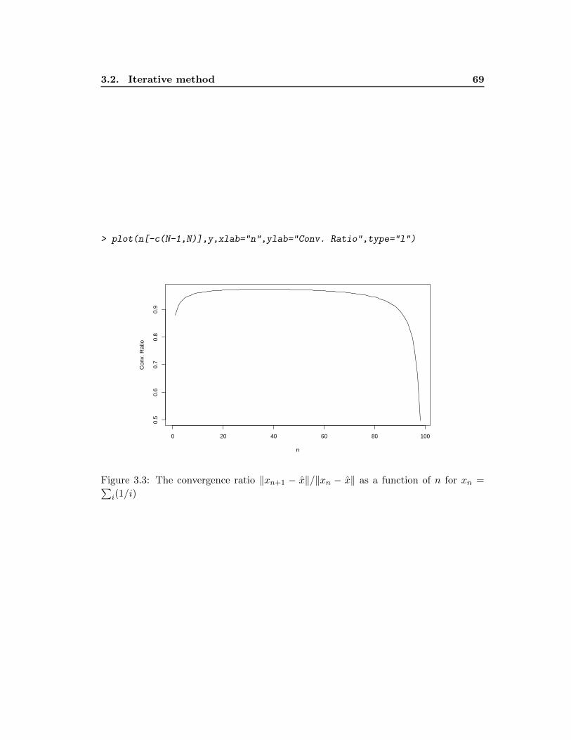
3.2. Iterative method 69
> plot(n[-c(N-1,N)],y,xlab="n",ylab="Conv. Ratio",type="l")
0 20 40 60 80 100
0.5
0.6
0.7
0.8
0.9
n
Con
v. R
atio
Figure 3.3: The convergence ratio ‖xn+1 − x‖/‖xn − x‖ as a function of n for xn =∑i(1/i)
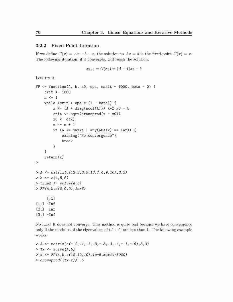
70 Chapter 3. Linear Equations and Iterative Methods
3.2.2 Fixed-Point Iteration
If we define G(x) = Ax − b + x, the solution to Ax = b is the fixed-point G(x) = x.
The following iteration, if it converges, will reach the solution:
xk+1 = G(xk) = (A+ I)xk − b
Lets try it:
FP <- function(A, b, x0, eps, maxit = 1000, beta = 0) {
crit <- 1000
n <- 1
while (crit > eps * (1 - beta)) {
x <- (A + diag(ncol(A))) %*% x0 - b
crit <- sqrt(crossprod(x - x0))
x0 <- c(x)
n <- n + 1
if (n >= maxit | any(abs(x) == Inf)) {
warning("No convergence")
break
}
}
return(x)
}
> A <- matrix(c(12,3,2,5,13,7,4,9,10),3,3)
> b <- c(4,5,6)
> trueX <- solve(A,b)
> FP(A,b,c(0,0,0),1e-6)
[,1]
[1,] -Inf
[2,] -Inf
[3,] -Inf
No luck! It does not converge. This method is quite bad because we have convergence
only if the modulus of the eigenvalues of (A+I) are less than 1. The following example
works.
> A <- matrix(c(-.2,.1,.1,.3,-.3,.3,.4,-.1,-.6),3,3)
> Tx <- solve(A,b)
> x <- FP(A,b,c(10,10,10),1e-5,maxit=5000)
> crossprod((Tx-x))^.5
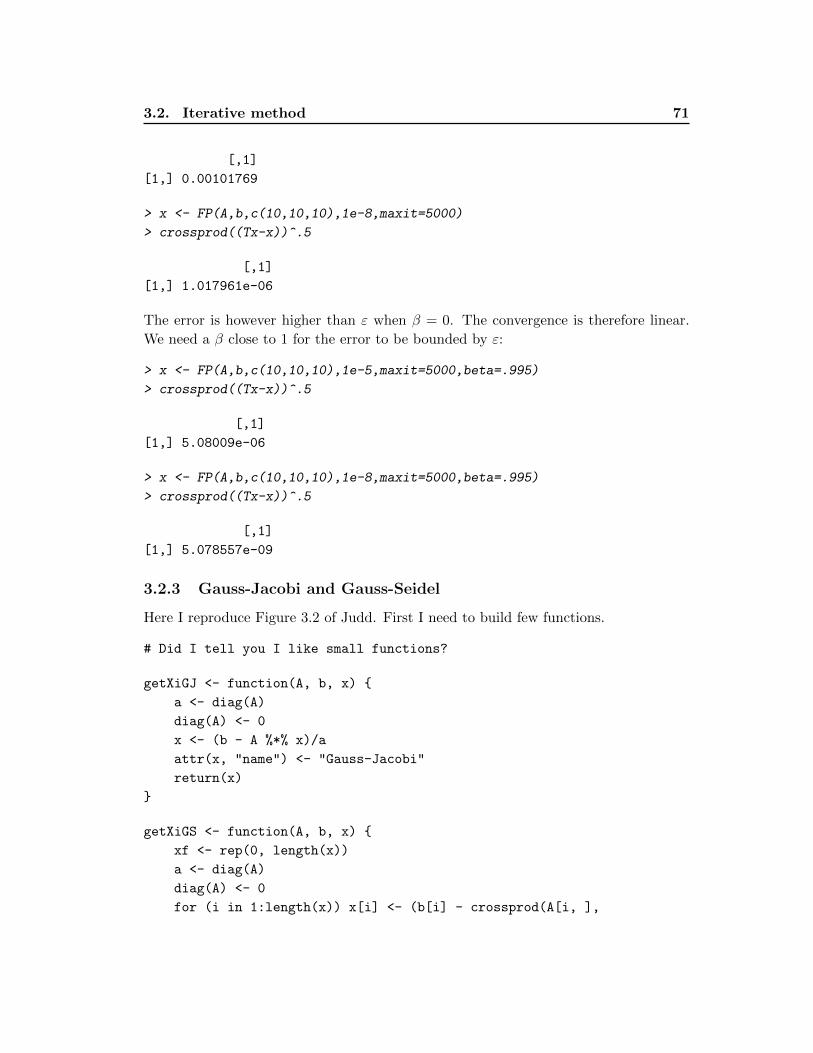
3.2. Iterative method 71
[,1]
[1,] 0.00101769
> x <- FP(A,b,c(10,10,10),1e-8,maxit=5000)
> crossprod((Tx-x))^.5
[,1]
[1,] 1.017961e-06
The error is however higher than ε when β = 0. The convergence is therefore linear.
We need a β close to 1 for the error to be bounded by ε:
> x <- FP(A,b,c(10,10,10),1e-5,maxit=5000,beta=.995)
> crossprod((Tx-x))^.5
[,1]
[1,] 5.08009e-06
> x <- FP(A,b,c(10,10,10),1e-8,maxit=5000,beta=.995)
> crossprod((Tx-x))^.5
[,1]
[1,] 5.078557e-09
3.2.3 Gauss-Jacobi and Gauss-Seidel
Here I reproduce Figure 3.2 of Judd. First I need to build few functions.
# Did I tell you I like small functions?
getXiGJ <- function(A, b, x) {
a <- diag(A)
diag(A) <- 0
x <- (b - A %*% x)/a
attr(x, "name") <- "Gauss-Jacobi"
return(x)
}
getXiGS <- function(A, b, x) {
xf <- rep(0, length(x))
a <- diag(A)
diag(A) <- 0
for (i in 1:length(x)) x[i] <- (b[i] - crossprod(A[i, ],
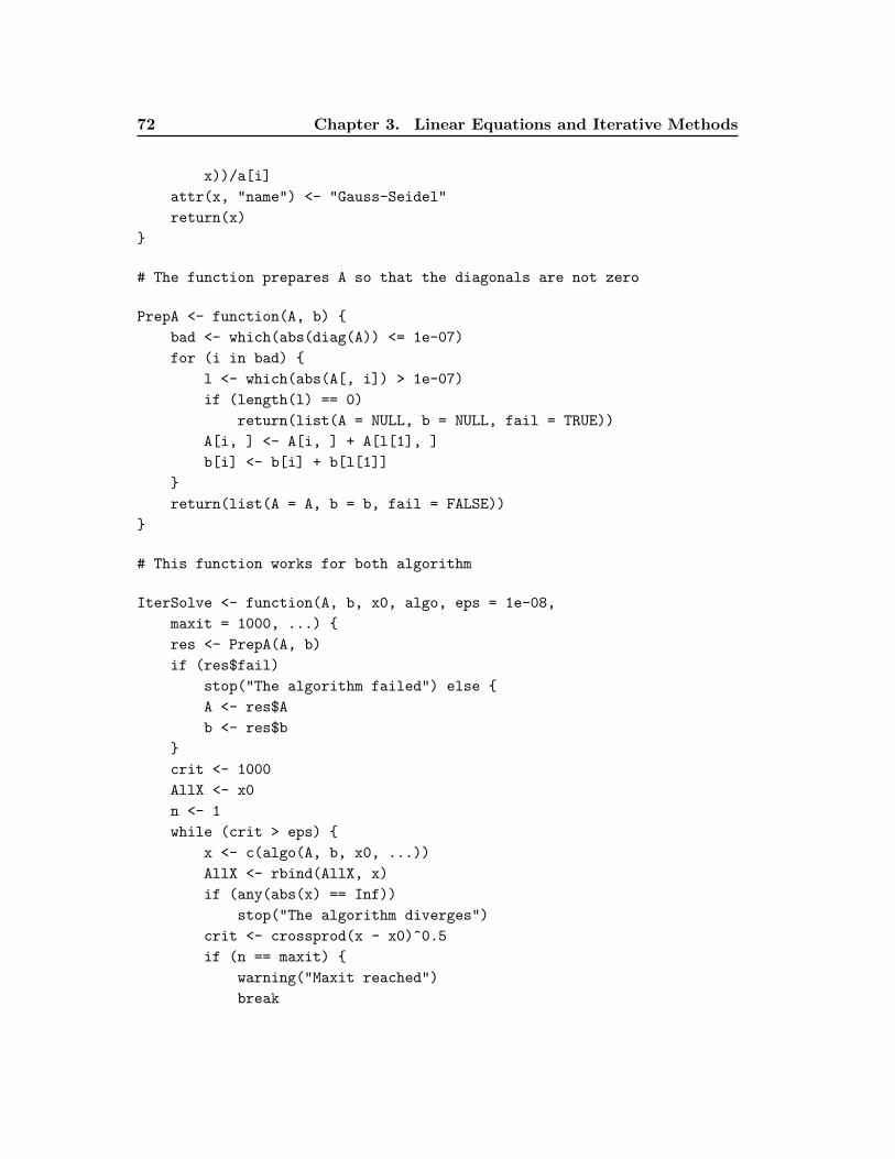
72 Chapter 3. Linear Equations and Iterative Methods
x))/a[i]
attr(x, "name") <- "Gauss-Seidel"
return(x)
}
# The function prepares A so that the diagonals are not zero
PrepA <- function(A, b) {
bad <- which(abs(diag(A)) <= 1e-07)
for (i in bad) {
l <- which(abs(A[, i]) > 1e-07)
if (length(l) == 0)
return(list(A = NULL, b = NULL, fail = TRUE))
A[i, ] <- A[i, ] + A[l[1], ]
b[i] <- b[i] + b[l[1]]
}
return(list(A = A, b = b, fail = FALSE))
}
# This function works for both algorithm
IterSolve <- function(A, b, x0, algo, eps = 1e-08,
maxit = 1000, ...) {
res <- PrepA(A, b)
if (res$fail)
stop("The algorithm failed") else {
A <- res$A
b <- res$b
}
crit <- 1000
AllX <- x0
n <- 1
while (crit > eps) {
x <- c(algo(A, b, x0, ...))
AllX <- rbind(AllX, x)
if (any(abs(x) == Inf))
stop("The algorithm diverges")
crit <- crossprod(x - x0)^0.5
if (n == maxit) {
warning("Maxit reached")
break
3.2. Iterative method 73
}
n <- n + 1
x0 <- x
}
if (n < maxit)
cat("\n", attr(x, "name"), "\nConverged after ", (n -
1), "iterations\n")
return(list(x = x, AllX = AllX))
}
We can try it with the previous matrix
> IterSolve(A,b,c(0,0,0),eps=1e-5,algo=getXiGJ)$x
Converged after 399 iterations
[1] -959.9998 -239.9999 -289.9999
> IterSolve(A,b,c(0,0,0),eps=1e-5,algo=getXiGS)$x
Converged after 169 iterations
[1] -959.9999 -240.0000 -290.0000
The second method is clearly faster than the first method, which is explained by the
fact that it uses the new information as soon as it is available. The two methods are
also much faster than the Fixed-point method. They also seem to converge better since
they both can solve the first problem we tried above with the Fixed-Point algorithm.
To see it, we even try very bad starting values:
> A <- matrix(c(12,3,2,5,13,7,4,9,10),3,3)
> b <- c(4,5,6)
> IterSolve(A,b,c(100,-100,50),eps=1e-5,algo=getXiGJ)$x
Converged after 104 iterations
[1] 0.16021871 -0.08840049 0.62983159
> IterSolve(A,b,c(100,-100,50),eps=1e-5,algo=getXiGS)$x
Converged after 22 iterations
[1] 0.16022332 -0.08840292 0.62983738
But there are examples in which the algorithms do not converge:
74 Chapter 3. Linear Equations and Iterative Methods
> set.seed(111)
> A <- matrix(rnorm(9),3,3)
> x1 <- try(IterSolve(A,b,c(100,-100,50),eps=1e-5,algo=getXiGS))
> cat(x1)
Error in IterSolve(A, b, c(100, -100, 50), eps = 1e-05, algo = getXiGS) :
The algorithm diverges
We’ll comeback to this convergence problem latter. We first want to see how we can
use the algorithm to analyze the dynamics of market going from any point to the
equilibrium. The model is:
p+ q = 10 (demand)
p− 2q = −2 (supply)
or (1 1
1 −2
)(p
q
)=
(10
−2
)First lets compare the two methods:
> A <- matrix(c(1,1,1,-2),2,2)
> b <- c(10,-2)
> res1 <- IterSolve(A,b,c(4,1),eps=1e-5,algo=getXiGS)
Converged after 21 iterations
> res2 <- IterSolve(A,b,c(4,1),eps=1e-5,algo=getXiGJ)
Converged after 40 iterations
> ans <- cbind(1:20,res1$AllX[1:20,],res2$AllX[1:20,])
> colnames(ans) <- c("n","p-(GS)","q-(GS)","p-(GJ)","q-(GJ)")
Table 3.2 shows some iteration results. We can see that the Gauss-Seidel method is
faster. The function plotEqui() creates something similar to Figure 3.2 of Judd. The
result is shown in Figure 3.4. The Gauss-Seidel method is slightly different because we
solve for the price first while Judd does the opposite. Also, the path in the book shows
movements between iteration while here we only show the final points.
plotEqui <- function(resGS, resGJ, A, b, n, Title = NULL,
xlab = NULL, ylab = NULL) {
x <- resGS$AllX[1:n, ]
x2 <- resGJ$AllX[1:n, ]
xsol <- solve(A, b)
3.2. Iterative method 75
n p-(GS) q-(GS) p-(GJ) q-(GJ)
1 1.0000 4.0000 1.0000 4.0000 1.0000
2 2.0000 9.0000 5.5000 9.0000 3.0000
3 3.0000 4.5000 3.2500 7.0000 5.5000
4 4.0000 6.7500 4.3750 4.5000 4.5000
5 5.0000 5.6250 3.8125 5.5000 3.2500
6 6.0000 6.1875 4.0938 6.7500 3.7500
7 7.0000 5.9062 3.9531 6.2500 4.3750
8 8.0000 6.0469 4.0234 5.6250 4.1250
9 10.0000 6.0117 4.0059 6.1875 3.9375
10 15.0000 5.9996 3.9998 6.0156 4.0234
11 20.0000 6.0000 4.0000 5.9941 4.0020
Table 3.2: The convergence of the algorithm of Gauss-Jacobi versus Gauss-Seidel for a
Demand-Supply example.
xlim <- c(0, 2 * xsol[2])
ylim <- c(0, 2 * xsol[1])
if (is.null(xlab))
xlab <- "Q"
if (is.null(ylab))
ylab <- "P"
curve((b[1] - A[1, 2] * x)/A[1, 1], 0, xlim[2], xlim = xlim,
ylim = ylim, xlab = xlab, ylab = ylab, bty = "n")
abline(b[2]/A[2, 1], -A[2, 2]/A[2, 1])
if (is.null(Title))
title("Dynamics of Demand and Supply Equilibrium") else title(Title)
for (i in 1:(n - 1)) {
text(x[i, 2], x[i, 1], i, col = 2, lwd = 4)
arrows(x[i, 2], x[i, 1], x[(i + 1), 2], x[(i + 1), 1],
col = 2)
}
text(x[n, 2], x[n, 1], n, col = 2, lwd = 4)
for (i in 1:(n - 1)) {
text(x2[i, 2], x2[i, 1], i, col = 4, lwd = 4)
arrows(x2[i, 2], x2[i, 1], x2[(i + 1), 2], x2[(i + 1),
1], lty = 2, col = 4)
}
76 Chapter 3. Linear Equations and Iterative Methods
> plotEqui(res1,res2,A,b,6)
0 2 4 6 8
02
46
810
12
Q
P
Dynamics of Demand and Supply Equilibrium
1
2
3
4
56
1
2
3
4
5
6
Gauss−SeidelGauss−Jacobi
Figure 3.4: Dynamics of the market using two types of iterative methods
text(x2[n, 2], x2[n, 1], n, col = 4, lwd = 4)
legend("top", c("Gauss-Seidel", "Gauss-Jacobi"), lty = c(1,
1), col = c(2, 4))
}
Using the dynamics of the model, we can see why in some cases, the iterative pro-
cedure does not converge. It is a nice example that uses the same argument as when
we analyze movements in differential equation models graphically. The method con-
verges because of the angle between the demand and the supply around the equilibrium.
Figure 3.5 shows what happens if the slope of the demand becomes -2.1:
> A <- matrix(c(1,1,2.1,-2),2,2)
> b <- c(10,-2)
> res1 <- IterSolve(A,b,c(2.2,3.8),eps=1e-5,algo=getXiGS)
> res2 <- IterSolve(A,b,c(2.2,3.8),eps=1e-5,algo=getXiGJ)
We would get a perpetual cycle if the ratio was 1 in absolute value (try it). Here
we are just solving a linear system. The non-convergence of the iterative methods does
not imply tt we do not have a solution:
> solve(A,b)
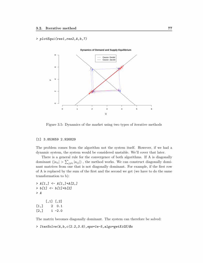
3.2. Iterative method 77
> plotEqui(res1,res2,A,b,7)
0 1 2 3 4 5 6
02
46
8
Q
PDynamics of Demand and Supply Equilibrium
12
3
4
5
6
7
12
3 4
56
7
Gauss−SeidelGauss−Jacobi
Figure 3.5: Dynamics of the market using two types of iterative methods
[1] 3.853659 2.926829
The problem comes from the algorithm not the system itself. However, if we had a
dynamic system, the system would be considered unstable. We’ll cover that later.
There is a general rule for the convergence of both algorithms. If A is diagonally
dominant (|aii| >∑
j 6=i |aij |) , the method works. We can construct diagonally domi-
nant matrices from one that is not diagonally dominant. For example, if the first row
of A is replaced by the sum of the first and the second we get (we have to do the same
transformation to b):
> A[1,] <- A[1,]+A[2,]
> b[1] <- b[1]+b[2]
> A
[,1] [,2]
[1,] 2 0.1
[2,] 1 -2.0
The matrix becomes diagonally dominant. The system can therefore be solved:
> IterSolve(A,b,c(2.2,3.8),eps=1e-5,algo=getXiGS)$x
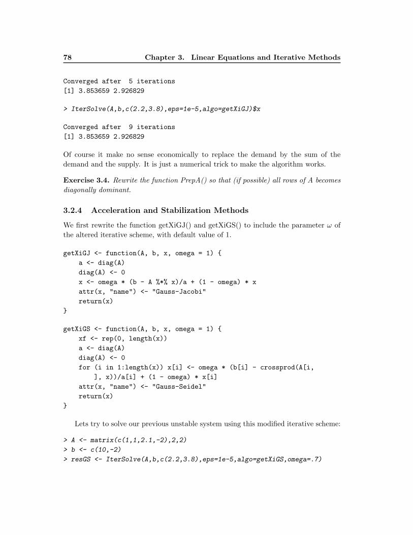
78 Chapter 3. Linear Equations and Iterative Methods
Converged after 5 iterations
[1] 3.853659 2.926829
> IterSolve(A,b,c(2.2,3.8),eps=1e-5,algo=getXiGJ)$x
Converged after 9 iterations
[1] 3.853659 2.926829
Of course it make no sense economically to replace the demand by the sum of the
demand and the supply. It is just a numerical trick to make the algorithm works.
Exercise 3.4. Rewrite the function PrepA() so that (if possible) all rows of A becomes
diagonally dominant.
3.2.4 Acceleration and Stabilization Methods
We first rewrite the function getXiGJ() and getXiGS() to include the parameter ω of
the altered iterative scheme, with default value of 1.
getXiGJ <- function(A, b, x, omega = 1) {
a <- diag(A)
diag(A) <- 0
x <- omega * (b - A %*% x)/a + (1 - omega) * x
attr(x, "name") <- "Gauss-Jacobi"
return(x)
}
getXiGS <- function(A, b, x, omega = 1) {
xf <- rep(0, length(x))
a <- diag(A)
diag(A) <- 0
for (i in 1:length(x)) x[i] <- omega * (b[i] - crossprod(A[i,
], x))/a[i] + (1 - omega) * x[i]
attr(x, "name") <- "Gauss-Seidel"
return(x)
}
Lets try to solve our previous unstable system using this modified iterative scheme:
> A <- matrix(c(1,1,2.1,-2),2,2)
> b <- c(10,-2)
> resGS <- IterSolve(A,b,c(2.2,3.8),eps=1e-5,algo=getXiGS,omega=.7)
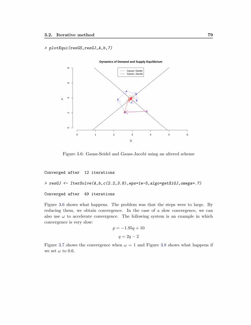
3.2. Iterative method 79
> plotEqui(resGS,resGJ,A,b,7)
0 1 2 3 4 5 6
02
46
8
Q
PDynamics of Demand and Supply Equilibrium
12
3 4567
12
3
45
67
Gauss−SeidelGauss−Jacobi
Figure 3.6: Gauss-Seidel and Gauss-Jacobi using an altered scheme
Converged after 12 iterations
> resGJ <- IterSolve(A,b,c(2.2,3.8),eps=1e-5,algo=getXiGJ,omega=.7)
Converged after 49 iterations
Figure 3.6 shows what happens. The problem was that the steps were to large. By
reducing them, we obtain convergence. In the case of a slow convergence, we can
also use ω to accelerate convergence. The following system is an example in which
convergence is very slow:
p = −1.95q + 10
q = 2q − 2
Figure 3.7 shows the convergence when ω = 1 and Figure 3.8 shows what happens if
we set ω to 0.6.
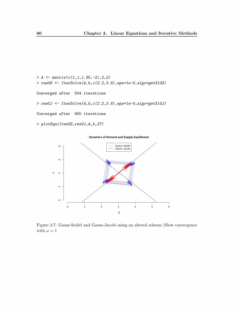
80 Chapter 3. Linear Equations and Iterative Methods
> A <- matrix(c(1,1,1.95,-2),2,2)
> resGS <- IterSolve(A,b,c(2.2,3.8),eps=1e-5,algo=getXiGS)
Converged after 504 iterations
> resGJ <- IterSolve(A,b,c(2.2,3.8),eps=1e-5,algo=getXiGJ)
Converged after 955 iterations
> plotEqui(resGS,resGJ,A,b,27)
0 1 2 3 4 5 6
02
46
8
Q
P
Dynamics of Demand and Supply Equilibrium
12
3
4
5
6
7
8
9
10
11
12
13
14
15
16
17
18
19
20
21
22
23
24
25
26
27
12
34
56
78
910
1112
1314
1516
1718
1920
2122
2324
2526
27
Gauss−SeidelGauss−Jacobi
Figure 3.7: Gauss-Seidel and Gauss-Jacobi using an altered scheme (Slow convergence
with ω = 1
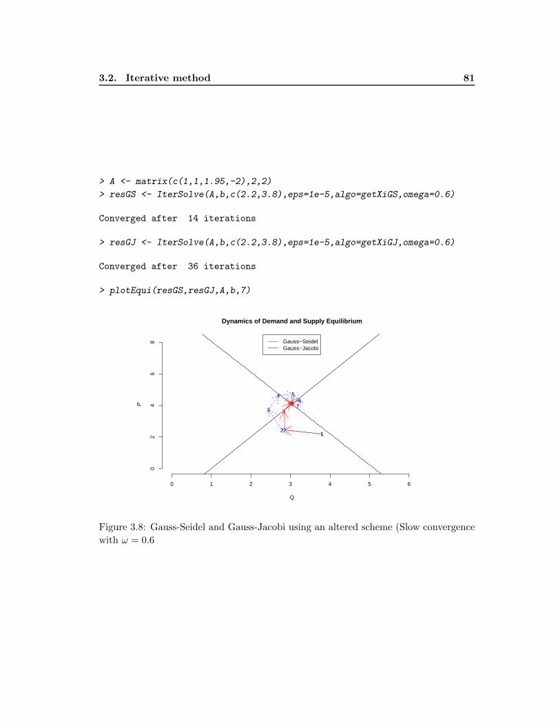
3.2. Iterative method 81
> A <- matrix(c(1,1,1.95,-2),2,2)
> resGS <- IterSolve(A,b,c(2.2,3.8),eps=1e-5,algo=getXiGS,omega=0.6)
Converged after 14 iterations
> resGJ <- IterSolve(A,b,c(2.2,3.8),eps=1e-5,algo=getXiGJ,omega=0.6)
Converged after 36 iterations
> plotEqui(resGS,resGJ,A,b,7)
0 1 2 3 4 5 6
02
46
8
Q
P
Dynamics of Demand and Supply Equilibrium
12
34567
12
3
4 56
7
Gauss−SeidelGauss−Jacobi
Figure 3.8: Gauss-Seidel and Gauss-Jacobi using an altered scheme (Slow convergence
with ω = 0.6
82 Chapter 3. Linear Equations and Iterative Methods
For Gauss-Seidel, we can obtain an optimal ω. If we write the iteration in matrix
form, we have:
xk+1 = M−1ω Nωxk + ωM−1ω b
where Mω = (D + ωL), Mω = (1 − ω)D − ωU , and U , L, and D are respectively the
element above the diagonal, the element below the diagonal and the diagonal of A. In
fact, we have A = U + L + D. The iterative scheme converges quickly if the largest
eigenvalues of (M−1ω Nω) in absolute value is small and less than 1. We therefore what
the value of ω that minimizes the largest eigenvalues. The following function selects
the optimal ω using a grid search. It is not efficient but it works:
getOmega <- function(A, from = 0.1, to = 1) {
w <- seq(to, from, len = 100)
ev <- vector()
D <- diag(diag(A))
U <- A * upper.tri(A)
L <- A * lower.tri(A)
for (i in 1:length(w)) {
M <- D + w[i] * L
N <- (1 - w[i]) * D - w[i] * U
ev[i] <- max(abs(eigen(solve(M, N))$val))
}
w[which.min(ev)]
}
We can verify with the last to systems:
> A <- matrix(c(1,1,2.1,-2),2,2)
> b <- c(10,-2)
> w <- getOmega(A,0,3)
> res1 <- IterSolve(A,b,c(2.2,3.8),eps=1e-5,algo=getXiGS,omega=w)
Converged after 9 iterations
> A <- matrix(c(1,1,1.95,-2),2,2)
> w <- getOmega(A,0,3)
> resGS <- IterSolve(A,b,c(2.2,3.8),eps=1e-5,algo=getXiGS,omega=w)
Converged after 10 iterations
It is in fact very fast with the optimal ω.
Exercise 3.5. Try to find the optimal ω for the Gauss-Jacobi method and write a
function like the one above to compute it. Compare the convergence of Gauss-Seidel
and Gauss-Jacobi using their optimal ω.
3.2. Iterative method 83
Exercise 3.6. Do the same for the fixed point algorithm.
We conclude this chapter with an example of Nash equilibrium computation. The
two reaction functions are:
p1 = 1 + 0.75p2
p2 = 2 + 0.8p1
In the following, we compare the convergence with different ω (find the optimal one),
and Figure 3.9 shows the case ω = 1.
> A <- matrix(c(1,-.8,-.75,1),2,2)
> b <- c(1,2)
> resGS <- IterSolve(A,b,c(2,1),eps=1e-5,algo=getXiGS)
Converged after 27 iterations
> resGJ <- IterSolve(A,b,c(2,1),eps=1e-5,algo=getXiGJ)
Converged after 50 iterations
> resGS2 <- IterSolve(A,b,c(2,1),eps=1e-5,algo=getXiGS,omega=.5)
Converged after 78 iterations
> resGJ2 <- IterSolve(A,b,c(2,1),eps=1e-5,algo=getXiGJ,omega=.5)
Converged after 96 iterations
In this example, reducing the value of ω does not help. Figure 3.10 shows us why. In
fact, we can accelerate the convergence by choosing a value greater than 1.
> resGS3 <- IterSolve(A,b,c(2,1),eps=1e-5,algo=getXiGS,omega=1.3)
Converged after 13 iterations
> resGJ3 <- IterSolve(A,b,c(2,1),eps=1e-5,algo=getXiGJ,omega=1.3)
It works for the Gauss-Seidel but not for the Gauss-Jacobi, which shows that the
optimal ω is not the same for the two algorithms. You can use the answer of Exercise
3.5 to show it.
Exercise 3.7. Answer questions 3, 6, 7 and 8 in Judd
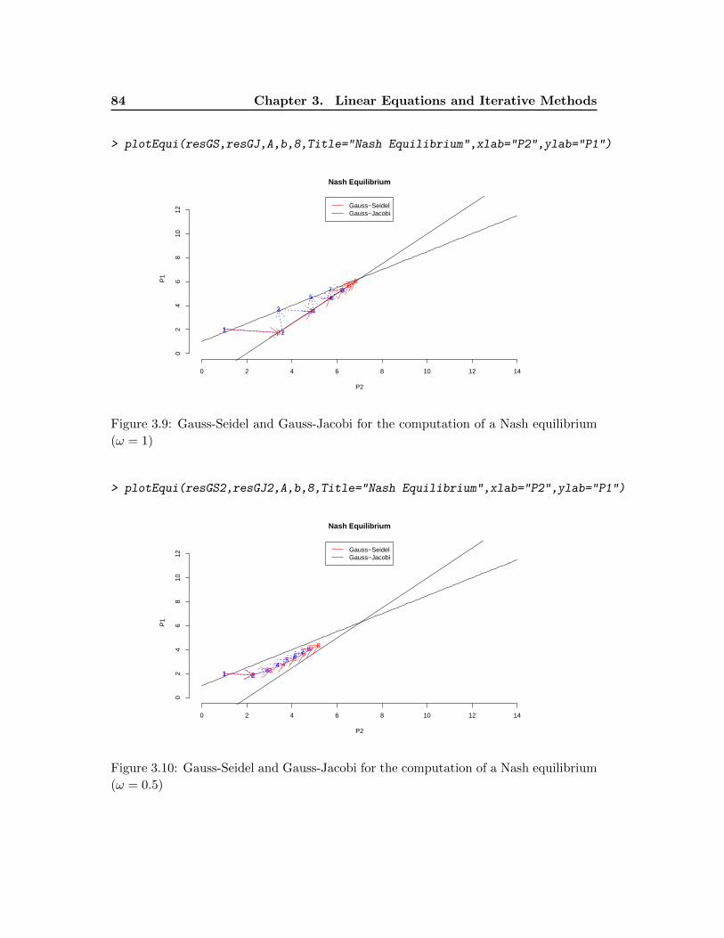
84 Chapter 3. Linear Equations and Iterative Methods
> plotEqui(resGS,resGJ,A,b,8,Title="Nash Equilibrium",xlab="P2",ylab="P1")
0 2 4 6 8 10 12 14
02
46
810
12
P2
P1
Nash Equilibrium
1 2
3
45
678
1 2
3 4
5 67 8
Gauss−SeidelGauss−Jacobi
Figure 3.9: Gauss-Seidel and Gauss-Jacobi for the computation of a Nash equilibrium
(ω = 1)
> plotEqui(resGS2,resGJ2,A,b,8,Title="Nash Equilibrium",xlab="P2",ylab="P1")
0 2 4 6 8 10 12 14
02
46
810
12
P2
P1
Nash Equilibrium
1 23
45
67
8
1 23
45
6 7 8
Gauss−SeidelGauss−Jacobi
Figure 3.10: Gauss-Seidel and Gauss-Jacobi for the computation of a Nash equilibrium
(ω = 0.5)
Chapter 4
Optimization
Contents
4.1 One-dimensional problems . . . . . . . . . . . . . . . . . . . . . . 85
4.2 Multidimensional Optimization . . . . . . . . . . . . . . . . . . . 94
4.2.1 A monopoly problem . . . . . . . . . . . . . . . . . . . . . . . . . . 94
4.2.2 Newton’s Method . . . . . . . . . . . . . . . . . . . . . . . . . . . . 97
4.2.3 Direction Set Methods . . . . . . . . . . . . . . . . . . . . . . . . . 101
4.2.4 Finite Differences . . . . . . . . . . . . . . . . . . . . . . . . . . . . 108
4.3 Constrained optimization . . . . . . . . . . . . . . . . . . . . . . . 109
4.4 Applications . . . . . . . . . . . . . . . . . . . . . . . . . . . . . . 112
4.4.1 Principal-Agent Problem . . . . . . . . . . . . . . . . . . . . . . . 112
4.4.2 Efficient Outcomes with Adverse Selection . . . . . . . . . . . . . . 112
4.4.3 Computing Nash Equilibrium. . . . . . . . . . . . . . . . . . . . . 113
4.4.4 Portfolio Problem . . . . . . . . . . . . . . . . . . . . . . . . . . . 114
4.4.5 Dynamic Optimization . . . . . . . . . . . . . . . . . . . . . . . . . 115
4.1 One-dimensional problems
Suppose we want to find a local minimum of the following function, for which the shape
is shown on Figure 4.1:
f(x) = sin (x− 0.04x2)− sin (x)
4
The easier way to find the solution is by the Bracketing method. We first need to
find three points, A, B and C, such that f(A) > f(B) and f(C) > f(B) as in Figure
4.1. The following function computes the solution using the Algorithm 4.1 of Judd (I
also create a print method. Why not keeping our good habits):
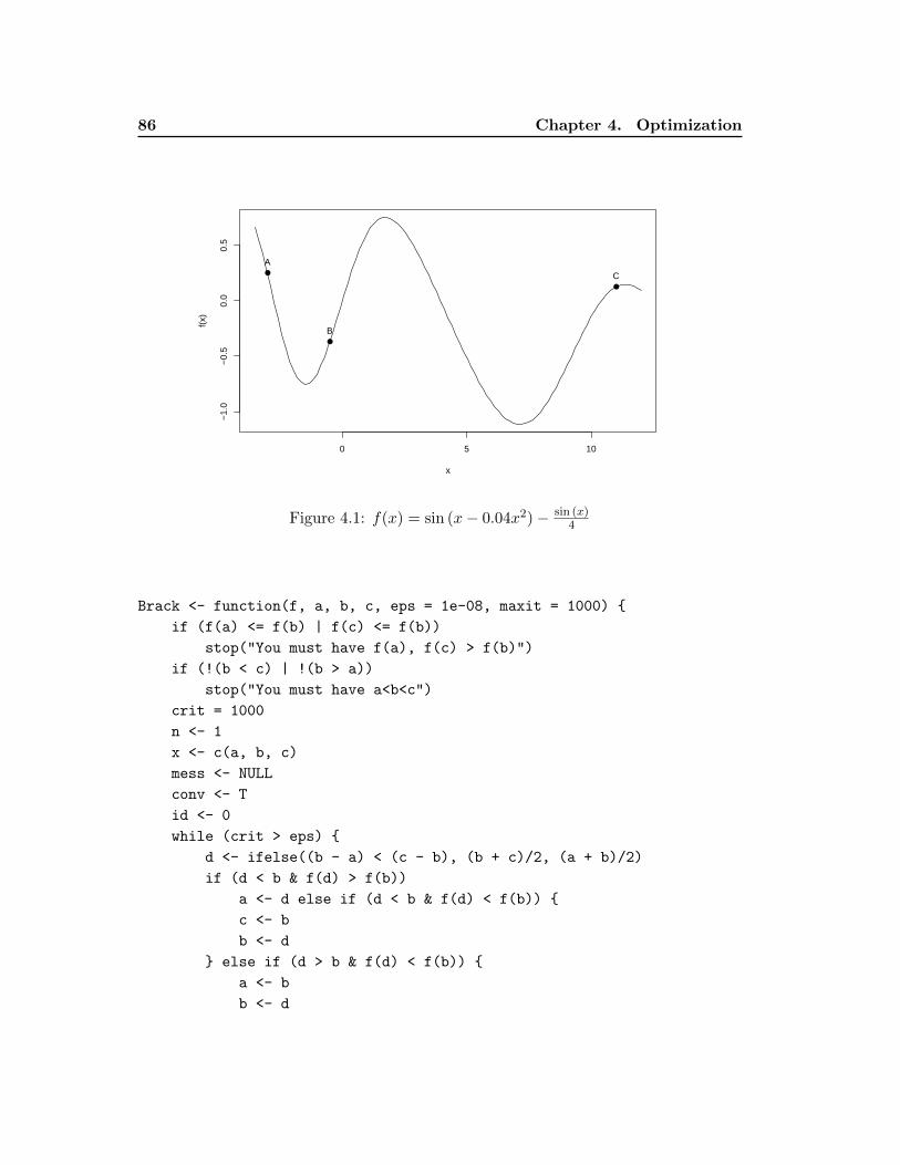
86 Chapter 4. Optimization
0 5 10
−1.
0−
0.5
0.0
0.5
x
f(x)
●
●
●
A
B
C
Figure 4.1: f(x) = sin (x− 0.04x2)− sin (x)4
Brack <- function(f, a, b, c, eps = 1e-08, maxit = 1000) {
if (f(a) <= f(b) | f(c) <= f(b))
stop("You must have f(a), f(c) > f(b)")
if (!(b < c) | !(b > a))
stop("You must have a<b<c")
crit = 1000
n <- 1
x <- c(a, b, c)
mess <- NULL
conv <- T
id <- 0
while (crit > eps) {
d <- ifelse((b - a) < (c - b), (b + c)/2, (a + b)/2)
if (d < b & f(d) > f(b))
a <- d else if (d < b & f(d) < f(b)) {
c <- b
b <- d
} else if (d > b & f(d) < f(b)) {
a <- b
b <- d
4.1. One-dimensional problems 87
} else c <- d
crit <- c - a
x <- rbind(x, c(a, b, c))
if (n >= maxit) {
mess <- paste("maxit(", maxit, ") reached", sep = "")
conv = F
break
}
n <- n + 1
}
n <- nrow(x)
ans <- list(obj = f(b), x = x, sol = b, name = "Bracketing Method",
conv = conv, prec = (x[n, 3] - x[n, 1]), mess = mess)
class(ans) <- "NonlinSol"
return(ans)
}
print.NonlinSol <- function(obj) {
n <- nrow(obj$x)
cat("\nMethod: ", obj$name, "\n")
if (obj$conv)
cat("Message: Converged after ", (n - 1), " iterations",
obj$mess, "\n\n") else cat("Message: ", obj$mess, "\n\n")
if (length(obj$sol) == 1)
cat("The solution is: ", obj$sol, ", and f(x) is ", obj$obj,
"\n") else {
cat("The solution is: \n")
if (is.null(names(obj$sol)))
names(obj$sol) <- paste("x", 1:length(obj$sol), sep = "")
for (i in 1:length(obj$sol)) cat(names(obj$sol)[i], " = ",
obj$sol[i], "\n")
cat("\nf(x) is ", obj$obj, "\n")
}
cat("Precision: ", obj$prec, "\n")
}
With the three points shown in Figure 4.1, the solution is:
> f <- function(x) sin(x-.04*x^2)-sin(x)/4
> res <- Brack(f,-3,-0.5,11)
> res
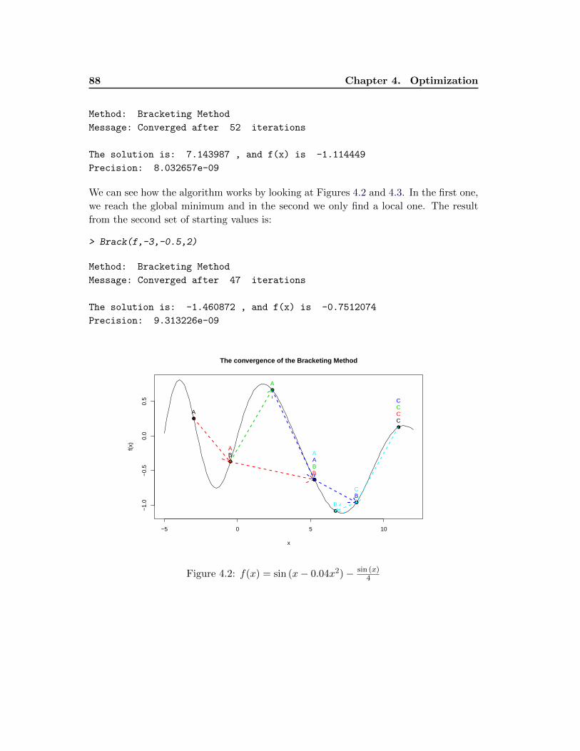
88 Chapter 4. Optimization
Method: Bracketing Method
Message: Converged after 52 iterations
The solution is: 7.143987 , and f(x) is -1.114449
Precision: 8.032657e-09
We can see how the algorithm works by looking at Figures 4.2 and 4.3. In the first one,
we reach the global minimum and in the second we only find a local one. The result
from the second set of starting values is:
> Brack(f,-3,-0.5,2)
Method: Bracketing Method
Message: Converged after 47 iterations
The solution is: -1.460872 , and f(x) is -0.7512074
Precision: 9.313226e-09
−5 0 5 10
−1.
0−
0.5
0.0
0.5
The convergence of the Bracketing Method
x
f(x)
●
●
●
A
B
C
A
B
C
●
●
A
B
C
●
A
B
C
●
●
A
B
C
●
●
Figure 4.2: f(x) = sin (x− 0.04x2)− sin (x)4
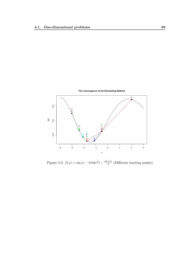
4.1. One-dimensional problems 89
−4 −3 −2 −1 0 1 2 3
−0.
50.
00.
5
The convergence of the Bracketing Method
x
f(x)
●
●
●
A
B
C
A
B
C
●
●
A
B
C
●
A
B
C●
AB
C●
Figure 4.3: f(x) = sin (x− 0.04x2)− sin (x)4 (Different starting points)
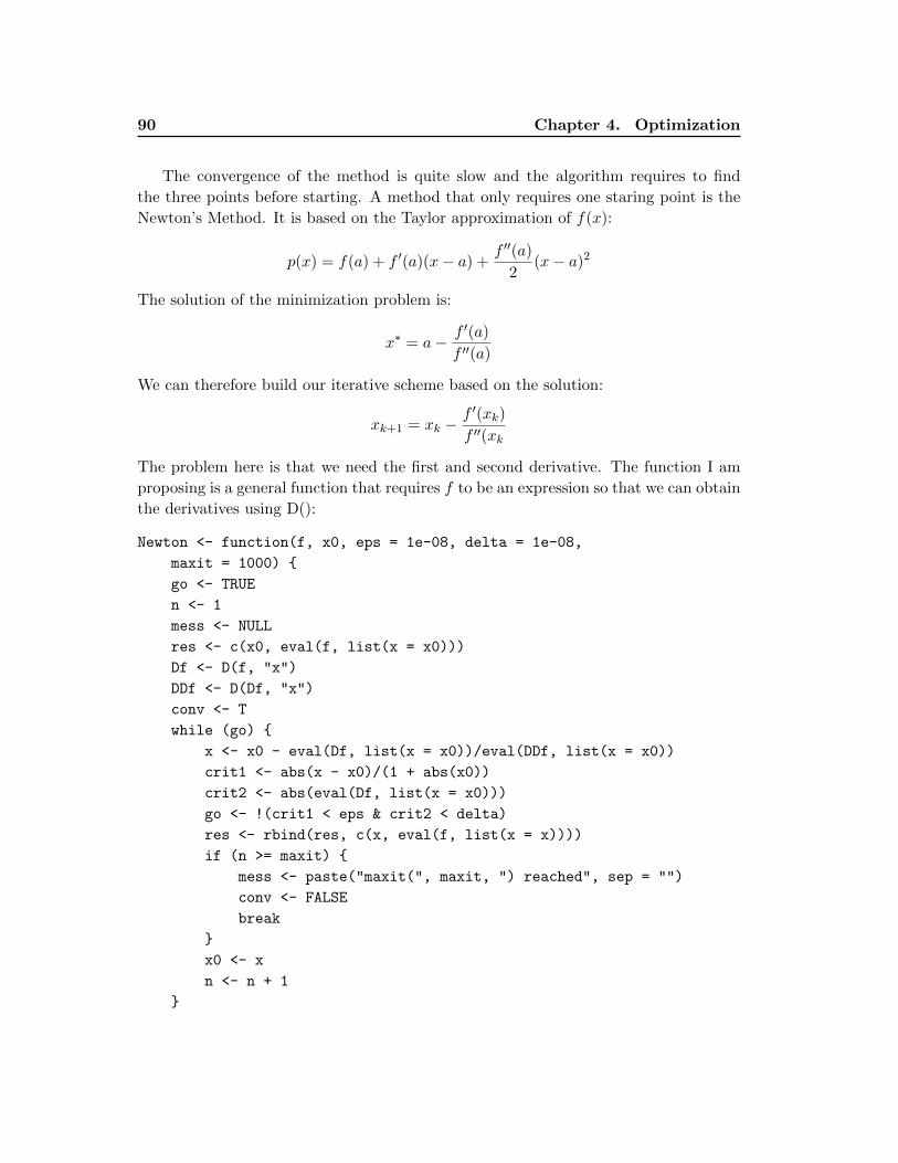
90 Chapter 4. Optimization
The convergence of the method is quite slow and the algorithm requires to find
the three points before starting. A method that only requires one staring point is the
Newton’s Method. It is based on the Taylor approximation of f(x):
p(x) = f(a) + f ′(a)(x− a) +f ′′(a)
2(x− a)2
The solution of the minimization problem is:
x∗ = a− f ′(a)
f ′′(a)
We can therefore build our iterative scheme based on the solution:
xk+1 = xk −f ′(xk)
f ′′(xk
The problem here is that we need the first and second derivative. The function I am
proposing is a general function that requires f to be an expression so that we can obtain
the derivatives using D():
Newton <- function(f, x0, eps = 1e-08, delta = 1e-08,
maxit = 1000) {
go <- TRUE
n <- 1
mess <- NULL
res <- c(x0, eval(f, list(x = x0)))
Df <- D(f, "x")
DDf <- D(Df, "x")
conv <- T
while (go) {
x <- x0 - eval(Df, list(x = x0))/eval(DDf, list(x = x0))
crit1 <- abs(x - x0)/(1 + abs(x0))
crit2 <- abs(eval(Df, list(x = x0)))
go <- !(crit1 < eps & crit2 < delta)
res <- rbind(res, c(x, eval(f, list(x = x))))
if (n >= maxit) {
mess <- paste("maxit(", maxit, ") reached", sep = "")
conv <- FALSE
break
}
x0 <- x
n <- n + 1
}
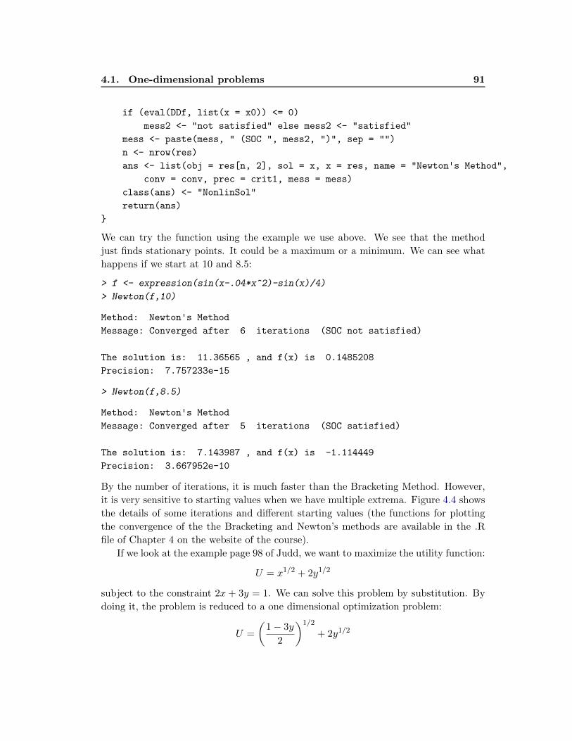
4.1. One-dimensional problems 91
if (eval(DDf, list(x = x0)) <= 0)
mess2 <- "not satisfied" else mess2 <- "satisfied"
mess <- paste(mess, " (SOC ", mess2, ")", sep = "")
n <- nrow(res)
ans <- list(obj = res[n, 2], sol = x, x = res, name = "Newton's Method",
conv = conv, prec = crit1, mess = mess)
class(ans) <- "NonlinSol"
return(ans)
}
We can try the function using the example we use above. We see that the method
just finds stationary points. It could be a maximum or a minimum. We can see what
happens if we start at 10 and 8.5:
> f <- expression(sin(x-.04*x^2)-sin(x)/4)
> Newton(f,10)
Method: Newton's Method
Message: Converged after 6 iterations (SOC not satisfied)
The solution is: 11.36565 , and f(x) is 0.1485208
Precision: 7.757233e-15
> Newton(f,8.5)
Method: Newton's Method
Message: Converged after 5 iterations (SOC satisfied)
The solution is: 7.143987 , and f(x) is -1.114449
Precision: 3.667952e-10
By the number of iterations, it is much faster than the Bracketing Method. However,
it is very sensitive to starting values when we have multiple extrema. Figure 4.4 shows
the details of some iterations and different starting values (the functions for plotting
the convergence of the the Bracketing and Newton’s methods are available in the .R
file of Chapter 4 on the website of the course).
If we look at the example page 98 of Judd, we want to maximize the utility function:
U = x1/2 + 2y1/2
subject to the constraint 2x+ 3y = 1. We can solve this problem by substitution. By
doing it, the problem is reduced to a one dimensional optimization problem:
U =
(1− 3y
2
)1/2
+ 2y1/2
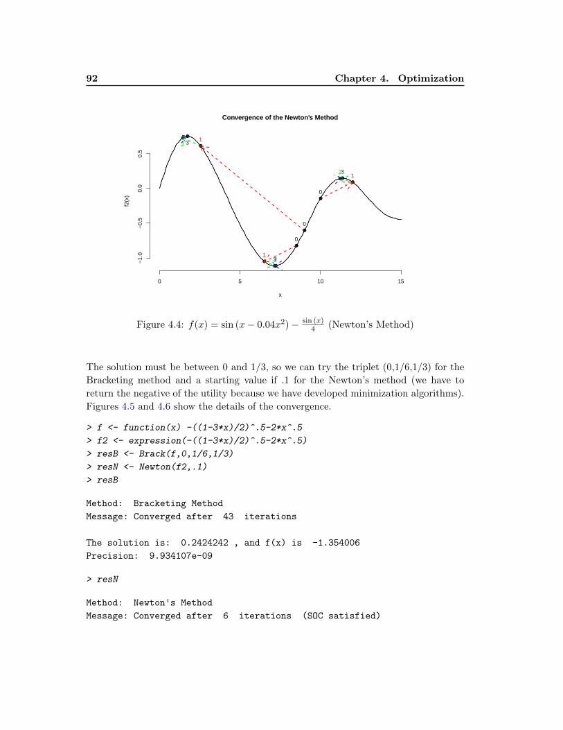
92 Chapter 4. Optimization
0 5 10 15
−1.
0−
0.5
0.0
0.5
Convergence of the Newton's Method
x
f2(x
)
●
●●●
0
123
●
●
● ●
0
12 3
●
●
●●
0
123
Figure 4.4: f(x) = sin (x− 0.04x2)− sin (x)4 (Newton’s Method)
The solution must be between 0 and 1/3, so we can try the triplet (0,1/6,1/3) for the
Bracketing method and a starting value if .1 for the Newton’s method (we have to
return the negative of the utility because we have developed minimization algorithms).
Figures 4.5 and 4.6 show the details of the convergence.
> f <- function(x) -((1-3*x)/2)^.5-2*x^.5
> f2 <- expression(-((1-3*x)/2)^.5-2*x^.5)
> resB <- Brack(f,0,1/6,1/3)
> resN <- Newton(f2,.1)
> resB
Method: Bracketing Method
Message: Converged after 43 iterations
The solution is: 0.2424242 , and f(x) is -1.354006
Precision: 9.934107e-09
> resN
Method: Newton's Method
Message: Converged after 6 iterations (SOC satisfied)
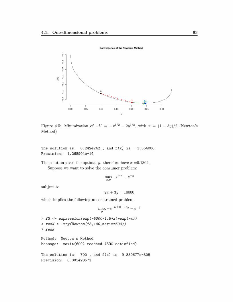
4.1. One-dimensional problems 93
0.00 0.05 0.10 0.15 0.20 0.25 0.30
−1.
3−
1.2
−1.
1−
1.0
−0.
9−
0.8
−0.
7
Convergence of the Newton's Method
x
f2(x
)
●
●●●●
0
1 234
Figure 4.5: Minimization of −U = −x1/2 − 2y1/2, with x = (1 − 3y)/2 (Newton’s
Method)
The solution is: 0.2424242 , and f(x) is -1.354006
Precision: 1.268904e-14
The solution gives the optimal y. therefore have x =0.1364.
Suppose we want to solve the consumer problem:
maxx,y−e−x − e−y
subject to
2x+ 3y = 10000
which implies the following unconstrained problem
maxy−e−5000+1.5y − e−y
> f3 <- expression(exp(-5000-1.5*x)+exp(-x))
> resN <- try(Newton(f3,100,maxit=600))
> resN
Method: Newton's Method
Message: maxit(600) reached (SOC satisfied)
The solution is: 700 , and f(x) is 9.859677e-305
Precision: 0.001428571
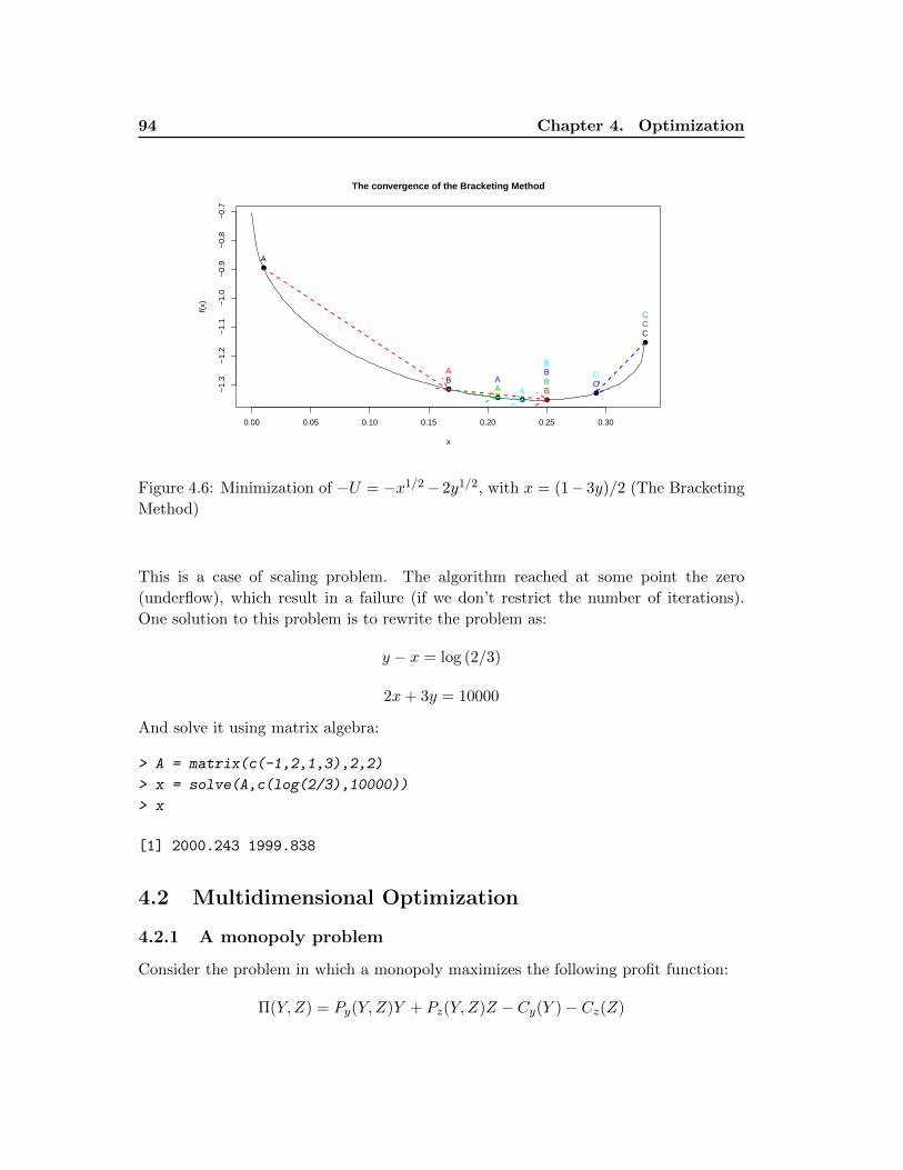
94 Chapter 4. Optimization
0.00 0.05 0.10 0.15 0.20 0.25 0.30
−1.
3−
1.2
−1.
1−
1.0
−0.
9−
0.8
−0.
7
The convergence of the Bracketing Method
x
f(x)
●
●
●
A
B
C
A
B
C
●
●
AB
C
●
AB
C●A
B
C
●
Figure 4.6: Minimization of −U = −x1/2− 2y1/2, with x = (1− 3y)/2 (The Bracketing
Method)
This is a case of scaling problem. The algorithm reached at some point the zero
(underflow), which result in a failure (if we don’t restrict the number of iterations).
One solution to this problem is to rewrite the problem as:
y − x = log (2/3)
2x+ 3y = 10000
And solve it using matrix algebra:
> A = matrix(c(-1,2,1,3),2,2)
> x = solve(A,c(log(2/3),10000))
> x
[1] 2000.243 1999.838
4.2 Multidimensional Optimization
4.2.1 A monopoly problem
Consider the problem in which a monopoly maximizes the following profit function:
Π(Y, Z) = Py(Y, Z)Y + Pz(Y,Z)Z − Cy(Y )− Cz(Z)
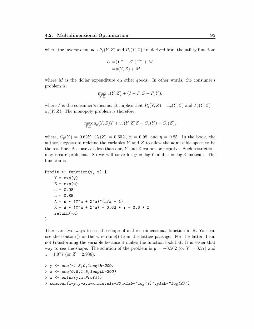
4.2. Multidimensional Optimization 95
where the inverse demands Py(Y,Z) and Pz(Y,Z) are derived from the utility function:
U =(Y α + Zα)η/α +M
=u(Y,Z) +M
where M is the dollar expenditure on other goods. In other words, the consumer’s
problem is:
maxY,Z
u(Y,Z) + (I − PzZ − PyY ),
where I is the consumer’s income. It implies that Py(Y,Z) = uy(Y,Z) and Pz(Y,Z) =
uz(Y,Z). The monopoly problem is therefore:
maxY,Z
uy(Y,Z)Y + uz(Y,Z)Z − Cy(Y )− Cz(Z),
where, Cy(Y ) = 0.62Y , Cz(Z) = 0.60Z, α = 0.98, and η = 0.85. In the book, the
author suggests to redefine the variables Y and Z to allow the admissible space to be
the real line. Because α is less than one, Y and Z cannot be negative. Such restrictions
may create problems. So we will solve for y = log Y and z = logZ instead. The
function is
Profit <- function(y, z) {
Y = exp(y)
Z = exp(z)
a = 0.98
n = 0.85
A = n * (Y^a + Z^a)^(n/a - 1)
R = A * (Y^a + Z^a) - 0.62 * Y - 0.6 * Z
return(-R)
}
There are two ways to see the shape of a three dimensional function in R. You can
use the contour() or the wireframe() from the lattice package. For the latter, I am
not transforming the variable because it makes the function look flat. It is easier that
way to see the shape. The solution of the problem is y = −0.562 (or Y = 0.57) and
z = 1.077 (or Z = 2.936).
> y <- seq(-1.5,0,length=200)
> z <- seq(0.5,1.5,length=200)
> x <- outer(y,z,Profit)
> contour(x=y,y=z,z=x,nlevels=20,xlab="log(Y)",ylab="log(Z)")
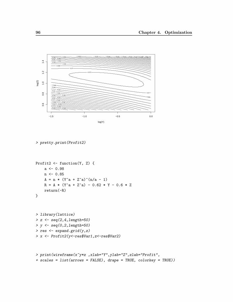
96 Chapter 4. Optimization
log(Y)
log(
Z)
−0.372
−0.37
−0.37
−0.368
−0.368
−0.366
−0.366
−0.364
−0.364
−0.362
−0.362
−0.36
−0.36
−0.358
−0.358
−0.356
−0.356
−0.354
−0.354
−0.352
−0.352
−0.35
−0.35
−0.348
−0.348
−0.346
−0.346
−0.344
−0.344
−0.342
−0.342
−0.34
−0.34
−0.338
−0.338
−0.336
−0.336
−0.334
−1.5 −1.0 −0.5 0.0
0.6
0.8
1.0
1.2
1.4
> pretty.print(Profit2)
Profit2 <- function(Y, Z) {
a <- 0.98
n <- 0.85
A = n * (Y^a + Z^a)^(n/a - 1)
R = A * (Y^a + Z^a) - 0.62 * Y - 0.6 * Z
return(-R)
}
> library(lattice)
> z <- seq(2,4,length=50)
> y <- seq(0,2,length=50)
> res <- expand.grid(y,z)
> x <- Profit2(y<-res$Var1,z<-res$Var2)
> print(wireframe(x~y*z ,xlab="Y",ylab="Z",zlab="Profit",
+ scales = list(arrows = FALSE), drape = TRUE, colorkey = TRUE))
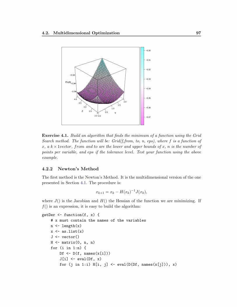
4.2. Multidimensional Optimization 97
0.0
0.5
1.0
1.5
2.0
2.0
2.5
3.0
3.5
4.0
−0.36
−0.34
−0.32
YZ
Profit
−0.37
−0.36
−0.35
−0.34
−0.33
−0.32
−0.31
−0.30
Exercise 4.1. Build an algorithm that finds the minimum of a function using the Grid
Search method. The function will be: Grid(f,from, to, n, eps), where f is a function of
x, a k× 1vector, from and to are the lower and upper bounds of x, n is the number of
points per variable, and eps if the tolerance level. Test your function using the above
example.
4.2.2 Newton’s Method
The first method is the Newton’s Method. It is the multidimensional version of the one
presented in Section 4.1. The procedure is:
xk+1 = xk −H(xk)−1J(xk),
where J() is the Jacobian and H() the Hessian of the function we are minimizing. If
f() is an expression, it is easy to build the algorithm:
getDer <- function(f, x) {
# x must contain the names of the variables
n <- length(x)
x <- as.list(x)
J <- vector()
H <- matrix(0, n, n)
for (i in 1:n) {
Df <- D(f, names(x[i]))
J[i] <- eval(Df, x)
for (j in 1:i) H[i, j] <- eval(D(Df, names(x[j])), x)
98 Chapter 4. Optimization
}
H[upper.tri(H)] <- H[lower.tri(H)]
dimnames(H) <- list(names(x), names(x))
names(J) <- names(x)
return(list(H = H, J = J))
}
MNewton <- function(f, x0, eps = 1e-08, delta = 1e-08,
maxit = 1000) {
n <- 1
conv = TRUE
mess <- NULL
fx <- eval(f, as.list(x0))
res <- c(x0, fx)
while (TRUE) {
resD <- getDer(f, x0)
H <- resD$H
J <- resD$J
x <- x0 - solve(H, J)
fx <- eval(f, as.list(x))
res <- rbind(res, c(x, fx))
crit1 <- sqrt(crossprod(x - x0))/(1 + sqrt(crossprod(x0)))
if (crit1 < eps) {
crit2 <- sqrt(crossprod(J))/(1 + abs(fx))
if (crit2 < delta)
break
}
if (n >= maxit) {
mess <- paste("maxit(", maxit, ") reached", sep = "")
conv = FALSE
break
}
x0 <- x
n <- n + 1
}
n <- nrow(res)
ans <- list(obj = res[n, ncol(res)], sol = x, x = res, name = "Newton's Method for Multidimensional Problems",
conv = conv, prec = crit1, mess = mess)
class(ans) <- "NonlinSol"
return(ans)
4.2. Multidimensional Optimization 99
}
We can then try it with the monopoly problem, and plot the result on a contour
plot:
> f <- expression(-0.85*(exp(y)^0.98+exp(z)^0.98)^(0.85/0.98-1)*(exp(y)^0.98 +
+ exp(z)^0.98)+0.62*exp(y)+0.6*exp(z))
> res <- MNewton(f,c(y=1,z=1))
> res
Method: Newton's Method for Multidimensional Problems
Message: Converged after 9 iterations
The solution is:
y = -0.5625466
z = 1.076945
f(x) is -0.3731764
Precision: 8.317925e-15
> y <- seq(-1,1.5,length=200)
> z <- seq(0,2,length=200)
> x <- outer(y,z,Profit)
> contour(x=y,y=z,z=x,nlevels=20,xlab="log(Y)",ylab="log(Z)")
> text(res$x[1:6,1],res$x[1:6,2]+.1,c("A","B","C","D","E","F"))
> points(res$x[1:6,1],res$x[1:6,2],pch=21,bg=2)
> lines(res$x[1:6,1],res$x[1:6,2],col=4)
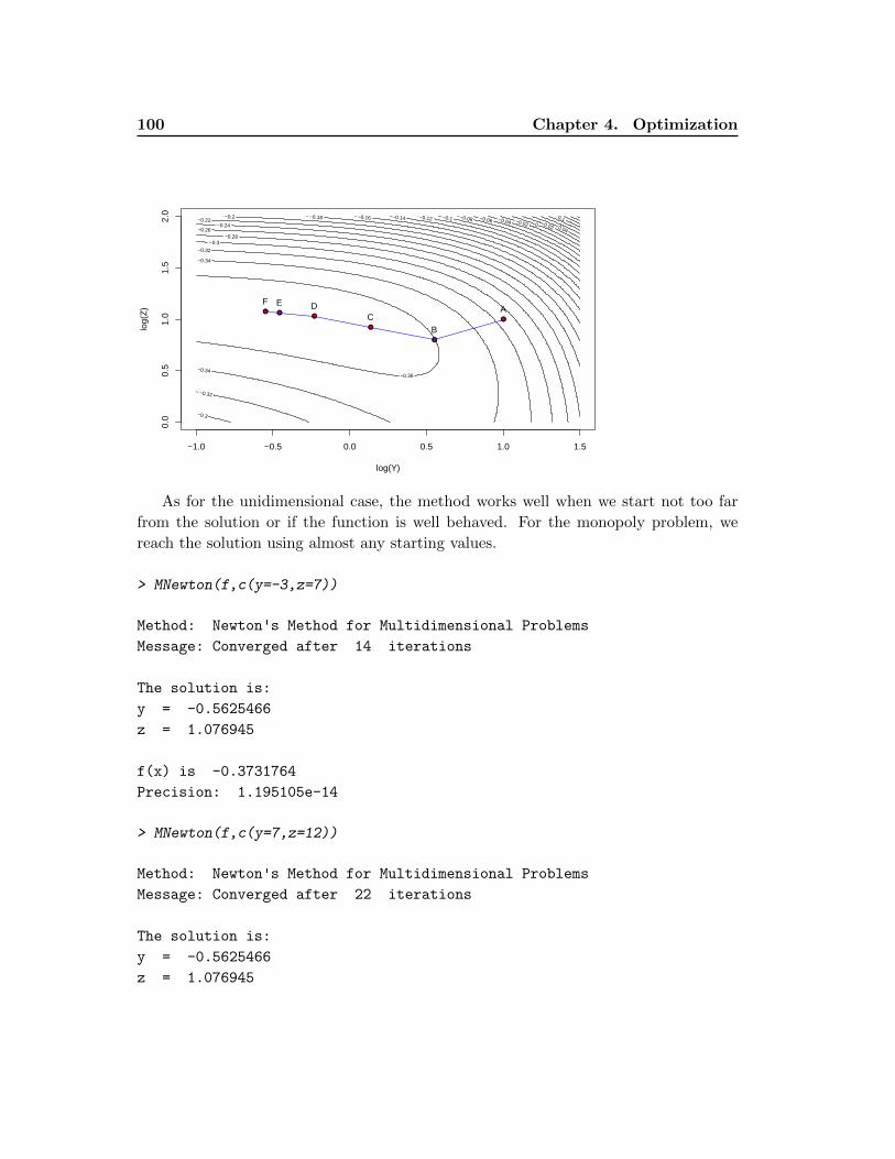
100 Chapter 4. Optimization
log(Y)
log(
Z)
−0.36 −0.34
−0.34
−0.32
−0.32
−0.3
−0.3 −0.28
−0.26 −0.24
−0.22 −0.2 −0.18 −0.16 −0.14 −0.12 −0.1 −0.08 −0.06 −0.04 −0.02 0 0.02 0.04
0.1
−1.0 −0.5 0.0 0.5 1.0 1.5
0.0
0.5
1.0
1.5
2.0
A
BC
DEF
●
●
●
●●●
As for the unidimensional case, the method works well when we start not too far
from the solution or if the function is well behaved. For the monopoly problem, we
reach the solution using almost any starting values.
> MNewton(f,c(y=-3,z=7))
Method: Newton's Method for Multidimensional Problems
Message: Converged after 14 iterations
The solution is:
y = -0.5625466
z = 1.076945
f(x) is -0.3731764
Precision: 1.195105e-14
> MNewton(f,c(y=7,z=12))
Method: Newton's Method for Multidimensional Problems
Message: Converged after 22 iterations
The solution is:
y = -0.5625466
z = 1.076945
4.2. Multidimensional Optimization 101
f(x) is -0.3731764
Precision: 4.912389e-09
Exercise 4.2. Write a function that combines the Newton’s and the Grid Search meth-
ods. It must use the grid search function you built for Exercise 4.1 to find a starting
vector. The latter is then, use to initiate the Newton’s Method. Try it with the monopoly
problem.
4.2.3 Direction Set Methods
Most optimization algorithms in R or any other numerical software are Direction Set
Methods. The general step is
xk+1 = xk + λksk,
where sk is a vector representing the search direction and λk is a scalar. All methods
differ in their respective choice of the search direction sk. On the other hand, the
method for computing λk is identical. If we want to minimize f(x), λk is defined as:
λk = arg minλf(xk + λsk)
Exercise 4.3. Write a function that compute λk. The function must have the form:
getLambda(f, x, s), where f is either an expression or a function (it is up to you). You
can also allow the two possibilities. You can verify your function by using the Profit
function. You should get (The function is hidden from the notes):
> print(getLambda(f,c(y=1,z=1),c(1,0)))
[1] -1.378165
We can summarize the different methods as follows (we consider the problem of
minimizing f(x), with x ∈ Rn:
� Coordinate Direction: sk = ei for i = 1, ..., n for each iteration (n directions
by iteration), where ei is the n× 1 vector with the ith element equals to 1 and all
others being equal to zero. (Always find a minimum when the function is smooth
but may be slow)
� Steepest Descent: sk = −J(xk) (Always find a minimum when the function is
smooth but may be slow)
� Newton’s Method with Line Search: sk = −H(xk)−1J(xk). As opposed to
the Newton’s Method, it will always go downhill.
102 Chapter 4. Optimization
� Broyden-Fletcher-Goldfarb-Shanno (BFGS): sk = −H(xk)−1J(xk), but
Hk is just an approximation of the hessian matrix. Starting with H0 = I, the
updates are:
Hk+1 = Hk −Hkzkz
′kHk
z′kHkzk+yky′k
y′kzk,
where zk = xk+1−xk and yk = J(xk+1)−J(xk). Whenever, y′kzk ≈ 0, Hk+1 = Hk.
� Conjugate Gradient: This method does not require the Hessian matrix; only
the Jacobian. The steps are: s0 = −J(x0) and
sk+1 = −J(xk+1) +‖J(xk+1)‖2
‖J(xk)‖2sk
and reset sk to −J(xk) every n iterations.
� Gauss-Newton Method for Nonlinear Least Squares: This method is spe-
cific to the following problem:
f(x) =T∑i=1
e2i (x),
where ei(x) is the ith residual (here, x is the vector of coefficients). Let the
T × n matrix J(x) be the Jacobian of the vector of residuals e(x). Than the
Gauss-Newton step is:
sk = −[J(xk)′J(xk)]
−1[J(xk)′e(xk)]
It is like the Newton’s Method but the Hessian is approximated by [J(xk)′J(xk)].
We first consider an application of the Gauss-Newton method. Lets consider the fol-
lowing Box-Cox transformation:
yλi − 1
λ= α+ βzi + ei
The vector x is {λ, α, β}. The ith line of J is then:
J(x)[i, ] =∂ei∂x
=(yλi [λ log (yi)−1]+1
λ2−1 −zi
)The following function applies the method but without line search:
GaussNewton <- function(f, x0, dat, eps = 1e-08, delta = 1e-08,
maxit = 1000) {
# f produces the vector of residuals
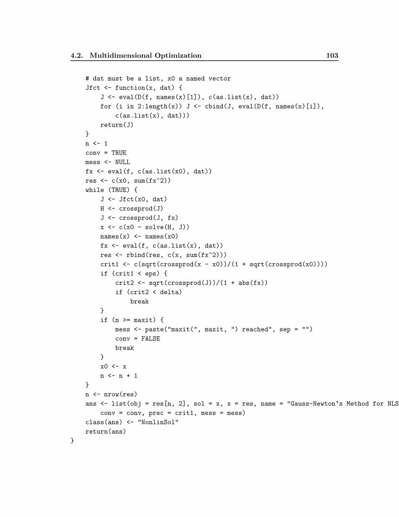
4.2. Multidimensional Optimization 103
# dat must be a list, x0 a named vector
Jfct <- function(x, dat) {
J <- eval(D(f, names(x)[1]), c(as.list(x), dat))
for (i in 2:length(x)) J <- cbind(J, eval(D(f, names(x)[i]),
c(as.list(x), dat)))
return(J)
}
n <- 1
conv = TRUE
mess <- NULL
fx <- eval(f, c(as.list(x0), dat))
res <- c(x0, sum(fx^2))
while (TRUE) {
J <- Jfct(x0, dat)
H <- crossprod(J)
J <- crossprod(J, fx)
x <- c(x0 - solve(H, J))
names(x) <- names(x0)
fx <- eval(f, c(as.list(x), dat))
res <- rbind(res, c(x, sum(fx^2)))
crit1 <- c(sqrt(crossprod(x - x0))/(1 + sqrt(crossprod(x0))))
if (crit1 < eps) {
crit2 <- sqrt(crossprod(J))/(1 + abs(fx))
if (crit2 < delta)
break
}
if (n >= maxit) {
mess <- paste("maxit(", maxit, ") reached", sep = "")
conv = FALSE
break
}
x0 <- x
n <- n + 1
}
n <- nrow(res)
ans <- list(obj = res[n, 2], sol = x, x = res, name = "Gauss-Newton's Method for NLS Problems",
conv = conv, prec = crit1, mess = mess)
class(ans) <- "NonlinSol"
return(ans)
}
104 Chapter 4. Optimization
We can see that the method does not work well for the Box-Cox estimation. Even
if we try different starting values, the algorithm diverges. The problem is that the
approximated Hessian becomes singular.
> f <- expression((y^l-1)/l -a -z*b)
> library(Ecdat)
> data(Consumption)
> C <- Consumption[,"ce"]
> z <- ts(1:length(C),freq=4,start=c(1947,1))
> dat <- list(y=C,z=z)
> res2 <- try(GaussNewton(f,c(l=.25,a=56,b=.2),dat,maxit=50,eps=1e-4))
> cat(res2[1])
Error in solve.default(H, J) :
system is computationally singular: reciprocal condition number = 1.11366e-16
In some cases, however, it works fine. Consider the following nonlinear model:
Yi = α1 + α2α3xi + α22zi + εi
In the following, I test the method using simulated data with α1 = 2, α2 = 3, and
α3 = 5. We can see that the method works fine.
> x <- rnorm(200)
> z <- rnorm(200)
> y <- 2+3*5*x+9*z+rnorm(200)
> f <- expression(y-a1-a2*a3*x-a2^2*z)
> dat <- list(y=y,x=x,z=z)
> x0 <- c(a1=0,a2=1,a3=1)
> res3 <- try(GaussNewton(f,x0,dat,maxit=100))
> print(res3)
Method: Gauss-Newton's Method for NLS Problems
Message: Converged after 7 iterations
The solution is:
a1 = 2.083002
a2 = 3.003899
a3 = 4.987922
f(x) is 3.003899
Precision: 1.38226e-16
4.2. Multidimensional Optimization 105
Exercise 4.4. Reproduce the results from Table 4.12 (Section 4.11) of Judd. You have
to compare the Newton and Gauss-Newton Methods for the following model:
y = αx1 + βx2 + β2x3 + ε
The residual sum of squares is:
S(α, β) =38.5− 5.24α− 7.56α2 − 6.10β + 9.96αβ
− 3.44β2 + 11.4αβ2 + 11.6β3 + 7.71β4
I conclude the section with a function to compute the BFGS method. For that
function, I require f to be a function and we have to provide a function that computes
the Jacobian. This setup does not exclude the use of symbolic derivatives. Here is an
example using the Box-Cox model:
fBC <- function(beta, dat) {
e <- expression((y^l - 1)/l - a1 - a2 * x)
sum(eval(e, c(as.list(beta), dat))^2)/2
}
DfBC <- function(beta, dat) {
e <- expression((y^l - 1)/l - a1 - a2 * x)
J <- eval(D(e, names(beta)[1]), c(as.list(beta), dat))
for (i in 2:length(beta)) J <- cbind(J, eval(D(e, names(beta)[i]),
c(as.list(beta), dat)))
et <- eval(e, c(as.list(beta), dat))
crossprod(J, et)
}
To allow both the case of theoretical and empirical models, The ”...” can be passed to
f and grad when we need to use data or set other parameter values.
BFGS <- function(f, x0, grad, eps = 1e-08, delta = 1e-08,
maxit = 100, ...) {
n <- 1
conv = TRUE
mess <- NULL
fx <- f(x0, ...)
res <- c(x0, fx)
H <- diag(length(x0))
while (TRUE) {
J <- grad(x0, ...)
s <- solve(H, -J)
106 Chapter 4. Optimization
l <- getLambda(f, x0, s, -50, 50, ...)
x <- x0 + l * s
names(x) <- names(x0)
fx <- f(x, ...)
res <- rbind(res, c(x, fx))
crit1 <- sqrt(crossprod(x - x0))/(1 + sqrt(crossprod(x0)))
if (crit1 < eps) {
crit2 <- sqrt(crossprod(J))/(1 + abs(fx))
if (crit2 < delta)
break
}
if (n >= maxit) {
mess <- paste("maxit(", maxit, ") reached", sep = "")
conv = FALSE
break
}
zk <- (x - x0)
yk <- J - grad(x, ...)
T1 <- c(t(yk) %*% zk)
T2 <- H %*% zk %*% t(zk) %*% H
T3 <- c(t(zk) %*% H %*% zk)
if (abs(T1) > 1e-07)
H <- H - T2/T3 + (yk %*% t(yk))/T1
n <- n + 1
x0 <- x
}
n <- nrow(res)
ans <- list(obj = res[n, 2], sol = x, x = res, name = "BFGS Method",
conv = conv, prec = crit1, mess = mess)
class(ans) <- "NonlinSol"
return(ans)
}
Lets try it on the monopoly problem:
f <- function(x) {
fexp <- expression(-0.85 * (exp(y)^0.98 + exp(z)^0.98)^(0.85/0.98 -
1) * (exp(y)^0.98 + exp(z)^0.98) + 0.62 * exp(y) + 0.6 *
exp(z))
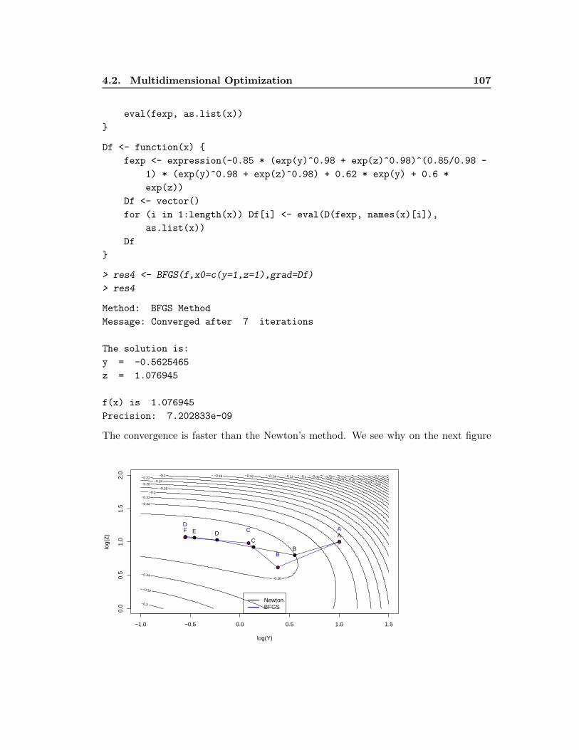
4.2. Multidimensional Optimization 107
eval(fexp, as.list(x))
}
Df <- function(x) {
fexp <- expression(-0.85 * (exp(y)^0.98 + exp(z)^0.98)^(0.85/0.98 -
1) * (exp(y)^0.98 + exp(z)^0.98) + 0.62 * exp(y) + 0.6 *
exp(z))
Df <- vector()
for (i in 1:length(x)) Df[i] <- eval(D(fexp, names(x)[i]),
as.list(x))
Df
}
> res4 <- BFGS(f,x0=c(y=1,z=1),grad=Df)
> res4
Method: BFGS Method
Message: Converged after 7 iterations
The solution is:
y = -0.5625465
z = 1.076945
f(x) is 1.076945
Precision: 7.202833e-09
The convergence is faster than the Newton’s method. We see why on the next figure
log(Y)
log(
Z)
−0.36 −0.34
−0.34
−0.32
−0.32
−0.3
−0.3 −0.28
−0.26 −0.24
−0.22 −0.2 −0.18 −0.16 −0.14 −0.12 −0.1 −0.08 −0.06 −0.04 −0.02 0 0.02 0.04
0.1
−1.0 −0.5 0.0 0.5 1.0 1.5
0.0
0.5
1.0
1.5
2.0
A
BC
DEF
●
●
●
●●●
A
B
CD
●
●
●
●
NewtonBFGS
108 Chapter 4. Optimization
Exercise 4.5. Answer the following questions
1. Write a function that solves optimization problems by the Coordinate Direction
with Line Search.
2. Write a function that solves optimization problems by the Steepest Descent with
Line Search.
3. Write a function that solves optimization problems by the Newton’s Method with
Line Search.
4. Write a function that solves optimization problems by the Conjugate Gradient
with Line Search.
5. Using the above monopoly example, Compare the Coordinate Direction, the Steep-
est Descent, the Newton’s Method with Line Search, the Conjugate Gradient, the
BFGS, and the Newton’s Method on a contour plot.
6. Compare your methods with optim() (compare the values of the coefficients and
the function, and the number of iterations)
Exercise 4.6. Answer question 1 of Chapter 4 of Judd (but do not use the Polytope
method).
Exercise 4.7. Answer question 2 of Chapter 4 of Judd.
4.2.4 Finite Differences
To avoid having to derive the analytical derivatives, it is possible to compute the
derivatives using finite differences. The derivatives are:
f ′(x) = limh→0
f(x+ h)− f(x)
h
We can approximate the derivatives by:
f ′(x) ≈ f(x+ h)− f(x)
h
for some small h. To be precise, h should be of order√εf |xc|, where εf is the rounding
error from evaluating f(x) and xc is [f(x)/f ′′(x)]1/2 (see [Press et al. 2007] page 229
for more details). This is meant to minimize the error. However, the following rule
works most of the time: h = max(ε1|x|, ε2), where ε1 can be around the square root of
the machine-epsilon (10−8), and ε2 is a not too small number. The latter is to prevent
problems when x is close to zero. If we set ε2 = 10−4, h will take that value whenever
|x| < 104. The following computes the numerical derivative of any function:
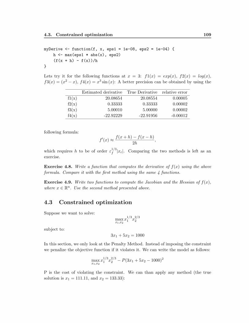
4.3. Constrained optimization 109
myDerive <- function(f, x, eps1 = 1e-08, eps2 = 1e-04) {
h <- max(eps1 * abs(x), eps2)
(f(x + h) - f(x))/h
}
Lets try it for the following functions at x = 3: f1(x) = exp(x), f2(x) = log(x),
f3(x) = (x2 − x), f4(x) = x3 sin (x): A better precision can be obtained by using the
Estimated derivative True Derivative relative error
f1(x) 20.08654 20.08554 0.00005
f2(x) 0.33333 0.33333 0.00002
f3(x) 5.00010 5.00000 0.00002
f4(x) -22.92229 -22.91956 -0.00012
following formula:
f ′(x) ≈ f(x+ h)− f(x− h)
2h,
which requires h to be of order ε1/3f |xc|. Comparing the two methods is left as an
exercise.
Exercise 4.8. Write a function that computes the derivative of f(x) using the above
formula. Compare it with the first method using the same 4 functions.
Exercise 4.9. Write two functions to compute the Jacobian and the Hessian of f(x),
where x ∈ Rn. Use the second method presented above.
4.3 Constrained optimization
Suppose we want to solve:
maxx1,x2
x1/31 x
2/32
subject to:
3x1 + 5x2 = 1000
In this section, we only look at the Penalty Method. Instead of imposing the constraint
we penalize the objective function if it violates it. We can write the model as follows:
maxx1,x2
x1/31 x
2/32 − P (3x1 + 5x2 − 1000)2
P is the cost of violating the constraint. We can than apply any method (the true
solution is x1 = 111.11, and x2 = 133.33):
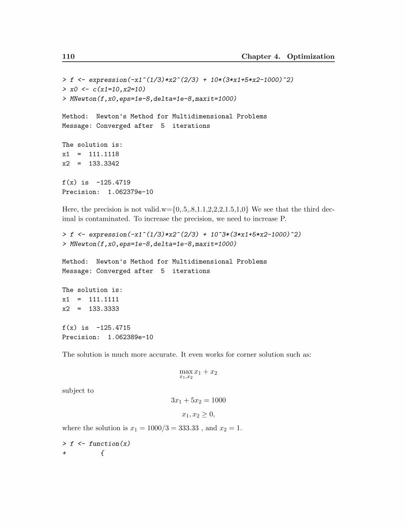
110 Chapter 4. Optimization
> f <- expression(-x1^(1/3)*x2^(2/3) + 10*(3*x1+5*x2-1000)^2)
> x0 <- c(x1=10,x2=10)
> MNewton(f,x0,eps=1e-8,delta=1e-8,maxit=1000)
Method: Newton's Method for Multidimensional Problems
Message: Converged after 5 iterations
The solution is:
x1 = 111.1118
x2 = 133.3342
f(x) is -125.4719
Precision: 1.062379e-10
Here, the precision is not valid.w={0,.5,.8,1.1,2,2,2,1.5,1,0} We see that the third dec-
imal is contaminated. To increase the precision, we need to increase P.
> f <- expression(-x1^(1/3)*x2^(2/3) + 10^3*(3*x1+5*x2-1000)^2)
> MNewton(f,x0,eps=1e-8,delta=1e-8,maxit=1000)
Method: Newton's Method for Multidimensional Problems
Message: Converged after 5 iterations
The solution is:
x1 = 111.1111
x2 = 133.3333
f(x) is -125.4715
Precision: 1.062389e-10
The solution is much more accurate. It even works for corner solution such as:
maxx1,x2
x1 + x2
subject to
3x1 + 5x2 = 1000
x1, x2 ≥ 0,
where the solution is x1 = 1000/3 = 333.33 , and x2 = 1.
> f <- function(x)
+ {
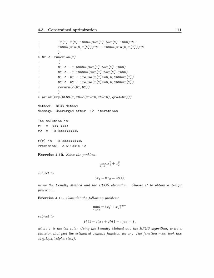
4.3. Constrained optimization 111
+ -x[1]-x[2]+1000*(3*x[1]+5*x[2]-1000)^2+
+ 1000*(min(0,x[2]))^2 + 1000*(min(0,x[1]))^2
+ }
> Df <- function(x)
+ {
+ D1 <- -1+6000*(3*x[1]+5*x[2]-1000)
+ D2 <- -1+10000*(3*x[1]+5*x[2]-1000)
+ D1 <- D1 + ifelse(x[1]>=0,0,2000*x[1])
+ D2 <- D2 + ifelse(x[2]>=0,0,2000*x[2])
+ return(c(D1,D2))
+ }
> print(try(BFGS(f,x0=c(x1=10,x2=10),grad=Df)))
Method: BFGS Method
Message: Converged after 12 iterations
The solution is:
x1 = 333.3339
x2 = -0.0003333336
f(x) is -0.0003333336
Precision: 2.611031e-12
Exercise 4.10. Solve the problem:
maxx1,x2
x21 + x22
subject to
6x1 + 8x2 = 4800,
using the Penalty Method and the BFGS algorithm. Choose P to obtain a 4-digit
precision.
Exercise 4.11. Consider the following problem:
maxx1,x2
= (xα1 + xα2 )η/α
subject to
P1(1− τ)x1 + P2(1− τ)x2 = I,
where τ is the tax rate. Using the Penalty Method and the BFGS algorithm, write a
function that plot the estimated demand function for x1. The function must look like
x1(p1,p2,t,alpha,eta,I).
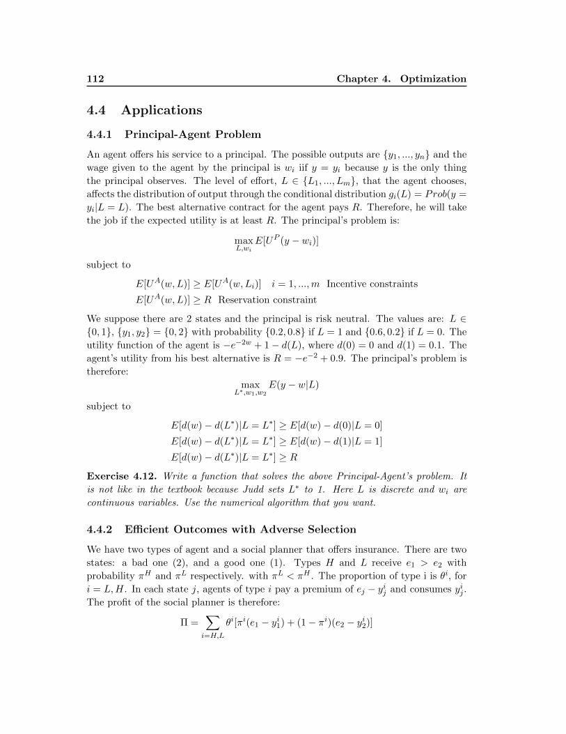
112 Chapter 4. Optimization
4.4 Applications
4.4.1 Principal-Agent Problem
An agent offers his service to a principal. The possible outputs are {y1, ..., yn} and the
wage given to the agent by the principal is wi iif y = yi because y is the only thing
the principal observes. The level of effort, L ∈ {L1, ..., Lm}, that the agent chooses,
affects the distribution of output through the conditional distribution gi(L) = Prob(y =
yi|L = L). The best alternative contract for the agent pays R. Therefore, he will take
the job if the expected utility is at least R. The principal’s problem is:
maxL,wi
E[UP (y − wi)]
subject to
E[UA(w,L)] ≥ E[UA(w,Li)] i = 1, ...,m Incentive constraints
E[UA(w,L)] ≥ R Reservation constraint
We suppose there are 2 states and the principal is risk neutral. The values are: L ∈{0, 1}, {y1, y2} = {0, 2} with probability {0.2, 0.8} if L = 1 and {0.6, 0.2} if L = 0. The
utility function of the agent is −e−2w + 1− d(L), where d(0) = 0 and d(1) = 0.1. The
agent’s utility from his best alternative is R = −e−2 + 0.9. The principal’s problem is
therefore:
maxL∗,w1,w2
E(y − w|L)
subject to
E[d(w)− d(L∗)|L = L∗] ≥ E[d(w)− d(0)|L = 0]
E[d(w)− d(L∗)|L = L∗] ≥ E[d(w)− d(1)|L = 1]
E[d(w)− d(L∗)|L = L∗] ≥ R
Exercise 4.12. Write a function that solves the above Principal-Agent’s problem. It
is not like in the textbook because Judd sets L∗ to 1. Here L is discrete and wi are
continuous variables. Use the numerical algorithm that you want.
4.4.2 Efficient Outcomes with Adverse Selection
We have two types of agent and a social planner that offers insurance. There are two
states: a bad one (2), and a good one (1). Types H and L receive e1 > e2 with
probability πH and πL respectively. with πL < πH . The proportion of type i is θi, for
i = L,H. In each state j, agents of type i pay a premium of ej − yij and consumes yij .
The profit of the social planner is therefore:
Π =∑i=H,L
θi[πi(e1 − yi1) + (1− πi)(e2 − yi2)]
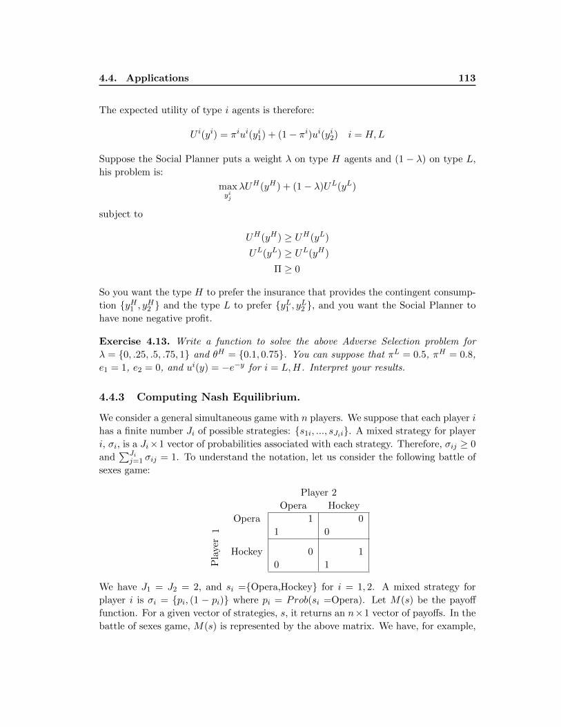
4.4. Applications 113
The expected utility of type i agents is therefore:
U i(yi) = πiui(yi1) + (1− πi)ui(yi2) i = H,L
Suppose the Social Planner puts a weight λ on type H agents and (1− λ) on type L,
his problem is:
maxyij
λUH(yH) + (1− λ)UL(yL)
subject to
UH(yH) ≥ UH(yL)
UL(yL) ≥ UL(yH)
Π ≥ 0
So you want the type H to prefer the insurance that provides the contingent consump-
tion {yH1 , yH2 } and the type L to prefer {yL1 , yL2 }, and you want the Social Planner to
have none negative profit.
Exercise 4.13. Write a function to solve the above Adverse Selection problem for
λ = {0, .25, .5, .75, 1} and θH = {0.1, 0.75}. You can suppose that πL = 0.5, πH = 0.8,
e1 = 1, e2 = 0, and ui(y) = −e−y for i = L,H. Interpret your results.
4.4.3 Computing Nash Equilibrium.
We consider a general simultaneous game with n players. We suppose that each player i
has a finite number Ji of possible strategies: {s1i, ..., sJii}. A mixed strategy for player
i, σi, is a Ji×1 vector of probabilities associated with each strategy. Therefore, σij ≥ 0
and∑Ji
j=1 σij = 1. To understand the notation, let us consider the following battle of
sexes game:
Player 2
Opera Hockey
1
Opera 1
1
0
0
Pla
yer
Hockey 0
0
1
1
We have J1 = J2 = 2, and si ={Opera,Hockey} for i = 1, 2. A mixed strategy for
player i is σi = {pi, (1 − pi)} where pi = Prob(si =Opera). Let M(s) be the payoff
function. For a given vector of strategies, s, it returns an n×1 vector of payoffs. In the
battle of sexes game, M(s) is represented by the above matrix. We have, for example,
114 Chapter 4. Optimization
M(Opera,Opera) = {1, 1}′, or M(Opera,Hockey) = {0, 0}′. We can generalize the
payoff function to include mixed strategies:
Mi(σ) =∑s
σ(s)Mi(s)
In our example, σi1 = pi and σi2 = (1− pi). Therefore:
M1(σ) =p1[p2(1) + (1− p2)(0)] + (1− p1)(p2(0) + (1− p2)(1)]
=p1p2 − (1− p1)(1− p2)=M2(σ),
We define Mi(sij , σ−i) as the payoff of player i when he plays the pure strategy sij and
the other players play the mixed strategy σ. Let us define the following function:
v(σ) =
n∑i=1
∑sij
[max{Mi(sij , σ−i)−Mi(σ), 0}]2
McKelvey (1992) shows that Nash Equilibia are both the minima and the zeros of v(σ).
In our example, M1(s11, σ−1) = p2 and M1(s12, σ−1) = (1− p2), and M2(s21, σ−2) = p1and M2(s22, σ−2) = (1− p1). Therefore,
v(σ) ≡v(p1, p2)
=[max{0, p2 −M1(σ)}]2 + [max{0, (1− p2)−M1(σ)}]2
+ [max{0, p1 −M2(σ)}]2 + [max{0, (1− p1)−M2(σ)}]2
It means that playing any pure strategy cannot result in payoffs higher than the payoffs
from playing the mixed strategy σ. The different equilibria are obtained by minimizing
v(σ) using different starting values, and by verifying that the solution that we obtain
implies that v(σ) = 0.
Exercise 4.14. Write a function that computes Nash equilibria for general 2-player
games. The number of possible strategies for each player may differ. The matrix of
payoffs can be a list of matrices (2 J1 × J2 matrices) or a 3 dimensional array (J1 ×J2 × 2). Use your function to answer question 4 of Chapter 4 of Judd.
4.4.4 Portfolio Problem
Consider an economy with n assets. Asset 1 is risk free and its price is p1 = 1. This
is a two period model in which investors are endowed with {e1, ..., en} units of assets
in period 1 and must choose how much to consume and how much to save for next
period consumption. They can purchase {ω1, ..., ωn} units of assets in period one at
4.4. Applications 115
{1, p2, ..., pn}. The assets will be worth {Z1, ..., Zn} in period 2. Period 1’s budget
constraint is therefore:
n∑i=1
piωi + c =
n∑i=1
piei
and the investors wants to maximize the expected utility of the two periods:
EU = u(c) + E
{u
(n∑i=1
ωiZi
)}
Exercise 4.15. Answer the following questions:
1. Solve the Portfolio Problem with: n = 3, u(c) = −e−ac, a ∈ {−0.5,−1,−5},Z1 = 2, Z2 ∼ {0.72, 0.92, 1.12, 1.32} with probabilities {1/4, 1/4, 1/4, 1/4}, Z3 ∼{0.86, 0.96, 1.06, 1.16} with probabilities {1/4, 1/4, 1/4, 1/4}, p = {1, .5, .5}, and
e = {2, 2, 2}. We also suppose that Z2 and Z3 are independent. Interpret your
results (for the all a’s).
2. Suppose now that p = {1, .3, .4}. Is there a solution to the problem? Why? Add
the assumption that short sales are forbidden and try to solve the problem for all
a’s. Interpret the results.
4.4.5 Dynamic Optimization
Consider an individual who lives n periods. At each period t, he allocates his wage wtbetween consumption ct and saving St. We suppose the interest rate r is constant. The
individual’s problem is to maximize his future discounted utility:
maxSt
T∑t=1
βtu(St−1(1 + r) + wt − St),
subject to S0 = ST = 0. We therefore have to solve for St, t = 1, ..., (T − 1).
Consider the following case: u(c) = −exp(−c), β = 0.9, r = .0.2, T = 10, and
w = {0, .5, .8, 1.1, 2, 2, 2, 1.5, 1, 0}. The following graph shows the result:
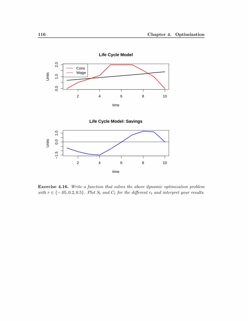
116 Chapter 4. Optimization
2 4 6 8 10
0.0
1.0
2.0
Life Cycle Model
time
Uni
ts
ConsWage
2 4 6 8 10
−1.
50.
01.
0
Life Cycle Model: Savings
time
Uni
ts
Exercise 4.16. Write a function that solves the above dynamic optimization problem
with r ∈ {−.05, 0.2, 0.5}. Plot St and Ct for the different rt and interpret your results.
Chapter 5
Nonlinear Equations
Contents
5.1 One-dimensional problems . . . . . . . . . . . . . . . . . . . . . . 117
5.1.1 The Bisection Method . . . . . . . . . . . . . . . . . . . . . . . . . 120
5.1.2 Newton’s Method . . . . . . . . . . . . . . . . . . . . . . . . . . . . 125
5.2 Multivariate Nonlinear Equations . . . . . . . . . . . . . . . . . 128
5.2.1 Newton’s Method . . . . . . . . . . . . . . . . . . . . . . . . . . . . 129
5.2.2 Gauss Methods . . . . . . . . . . . . . . . . . . . . . . . . . . . . . 130
5.2.3 Broyden’s Method . . . . . . . . . . . . . . . . . . . . . . . . . . . 132
5.2.4 The nleqslv package . . . . . . . . . . . . . . . . . . . . . . . . . . 133
5.2.5 Example . . . . . . . . . . . . . . . . . . . . . . . . . . . . . . . . . 134
5.1 One-dimensional problems
Consider the problem of computing the yield to maturity of a coupon-bond with semi-
annual coupon of $50, par value of $1,000, maturity of 10 years, and a price of $850.
The formula that links the bond price and the yield is:
P =C
y/2+
(PAR− C
y/2
)(1 + y/2)−2T ,
where C is the coupon, y is the yield to maturity compounded semiannually, T is the
maturity, and PAR is the par value. In our problem, we want to solve:
f(y) = 850− 50
y/2−(
1000− 50
y/2
)(1 + y/2)−20 = 0
The following graph shows the shape of f(y):
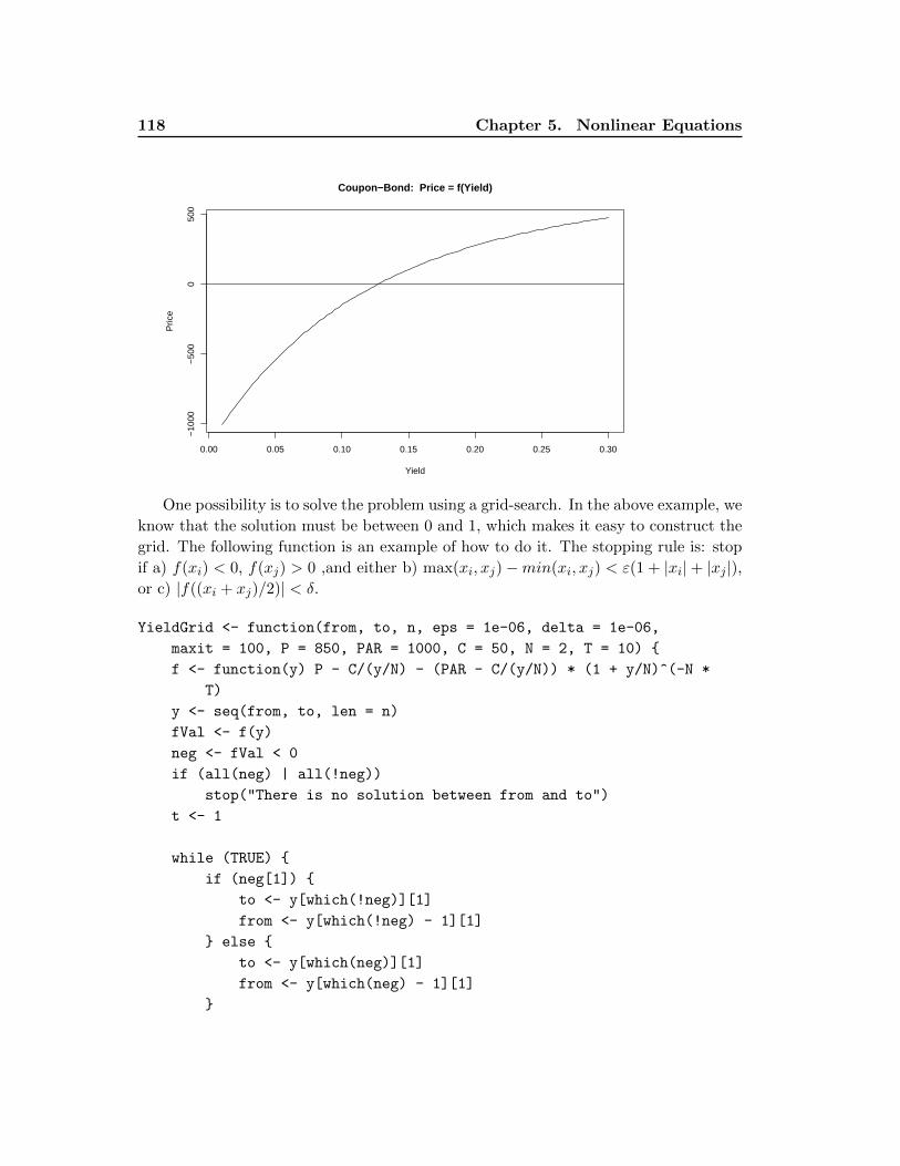
118 Chapter 5. Nonlinear Equations
0.00 0.05 0.10 0.15 0.20 0.25 0.30
−10
00−
500
050
0Coupon−Bond: Price = f(Yield)
Yield
Pric
e
One possibility is to solve the problem using a grid-search. In the above example, we
know that the solution must be between 0 and 1, which makes it easy to construct the
grid. The following function is an example of how to do it. The stopping rule is: stop
if a) f(xi) < 0, f(xj) > 0 ,and either b) max(xi, xj)−min(xi, xj) < ε(1 + |xi|+ |xj |),or c) |f((xi + xj)/2)| < δ.
YieldGrid <- function(from, to, n, eps = 1e-06, delta = 1e-06,
maxit = 100, P = 850, PAR = 1000, C = 50, N = 2, T = 10) {
f <- function(y) P - C/(y/N) - (PAR - C/(y/N)) * (1 + y/N)^(-N *
T)
y <- seq(from, to, len = n)
fVal <- f(y)
neg <- fVal < 0
if (all(neg) | all(!neg))
stop("There is no solution between from and to")
t <- 1
while (TRUE) {
if (neg[1]) {
to <- y[which(!neg)][1]
from <- y[which(!neg) - 1][1]
} else {
to <- y[which(neg)][1]
from <- y[which(neg) - 1][1]
}
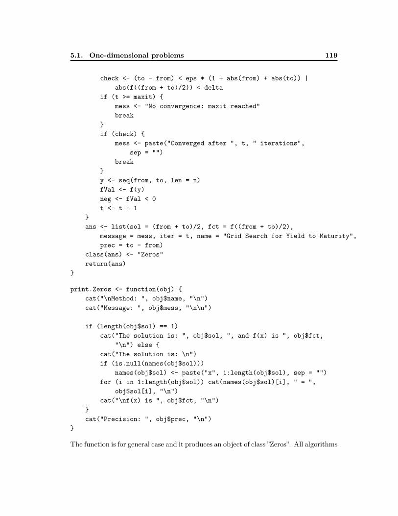
5.1. One-dimensional problems 119
check <- (to - from) < eps * (1 + abs(from) + abs(to)) |
abs(f((from + to)/2)) < delta
if (t >= maxit) {
mess <- "No convergence: maxit reached"
break
}
if (check) {
mess <- paste("Converged after ", t, " iterations",
sep = "")
break
}
y <- seq(from, to, len = n)
fVal <- f(y)
neg <- fVal < 0
t <- t + 1
}
ans <- list(sol = (from + to)/2, fct = f((from + to)/2),
message = mess, iter = t, name = "Grid Search for Yield to Maturity",
prec = to - from)
class(ans) <- "Zeros"
return(ans)
}
print.Zeros <- function(obj) {
cat("\nMethod: ", obj$name, "\n")
cat("Message: ", obj$mess, "\n\n")
if (length(obj$sol) == 1)
cat("The solution is: ", obj$sol, ", and f(x) is ", obj$fct,
"\n") else {
cat("The solution is: \n")
if (is.null(names(obj$sol)))
names(obj$sol) <- paste("x", 1:length(obj$sol), sep = "")
for (i in 1:length(obj$sol)) cat(names(obj$sol)[i], " = ",
obj$sol[i], "\n")
cat("\nf(x) is ", obj$fct, "\n")
}
cat("Precision: ", obj$prec, "\n")
}
The function is for general case and it produces an object of class ”Zeros”. All algorithms
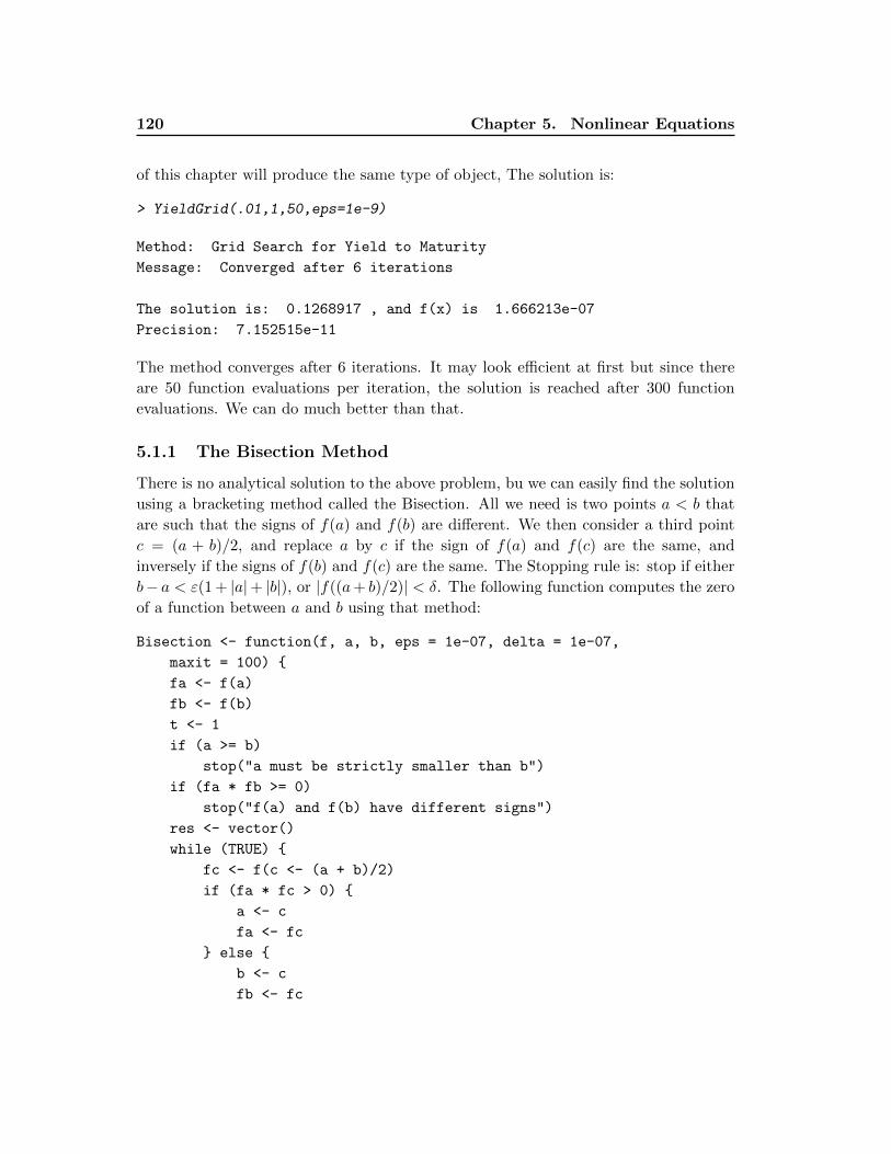
120 Chapter 5. Nonlinear Equations
of this chapter will produce the same type of object, The solution is:
> YieldGrid(.01,1,50,eps=1e-9)
Method: Grid Search for Yield to Maturity
Message: Converged after 6 iterations
The solution is: 0.1268917 , and f(x) is 1.666213e-07
Precision: 7.152515e-11
The method converges after 6 iterations. It may look efficient at first but since there
are 50 function evaluations per iteration, the solution is reached after 300 function
evaluations. We can do much better than that.
5.1.1 The Bisection Method
There is no analytical solution to the above problem, bu we can easily find the solution
using a bracketing method called the Bisection. All we need is two points a < b that
are such that the signs of f(a) and f(b) are different. We then consider a third point
c = (a + b)/2, and replace a by c if the sign of f(a) and f(c) are the same, and
inversely if the signs of f(b) and f(c) are the same. The Stopping rule is: stop if either
b− a < ε(1 + |a|+ |b|), or |f((a+ b)/2)| < δ. The following function computes the zero
of a function between a and b using that method:
Bisection <- function(f, a, b, eps = 1e-07, delta = 1e-07,
maxit = 100) {
fa <- f(a)
fb <- f(b)
t <- 1
if (a >= b)
stop("a must be strictly smaller than b")
if (fa * fb >= 0)
stop("f(a) and f(b) have different signs")
res <- vector()
while (TRUE) {
fc <- f(c <- (a + b)/2)
if (fa * fc > 0) {
a <- c
fa <- fc
} else {
b <- c
fb <- fc
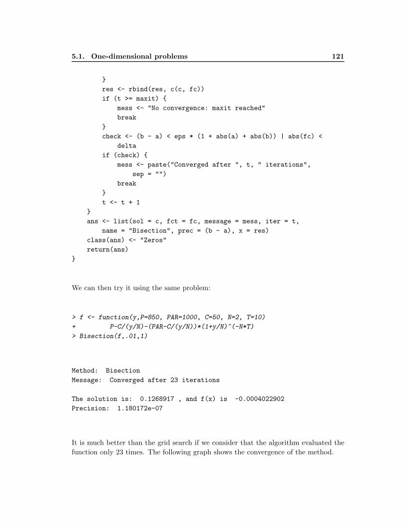
5.1. One-dimensional problems 121
}
res <- rbind(res, c(c, fc))
if (t >= maxit) {
mess <- "No convergence: maxit reached"
break
}
check <- (b - a) < eps * (1 + abs(a) + abs(b)) | abs(fc) <
delta
if (check) {
mess <- paste("Converged after ", t, " iterations",
sep = "")
break
}
t <- t + 1
}
ans <- list(sol = c, fct = fc, message = mess, iter = t,
name = "Bisection", prec = (b - a), x = res)
class(ans) <- "Zeros"
return(ans)
}
We can then try it using the same problem:
> f <- function(y,P=850, PAR=1000, C=50, N=2, T=10)
+ P-C/(y/N)-(PAR-C/(y/N))*(1+y/N)^(-N*T)
> Bisection(f,.01,1)
Method: Bisection
Message: Converged after 23 iterations
The solution is: 0.1268917 , and f(x) is -0.0004022902
Precision: 1.180172e-07
It is much better than the grid search if we consider that the algorithm evaluated the
function only 23 times. The following graph shows the convergence of the method.
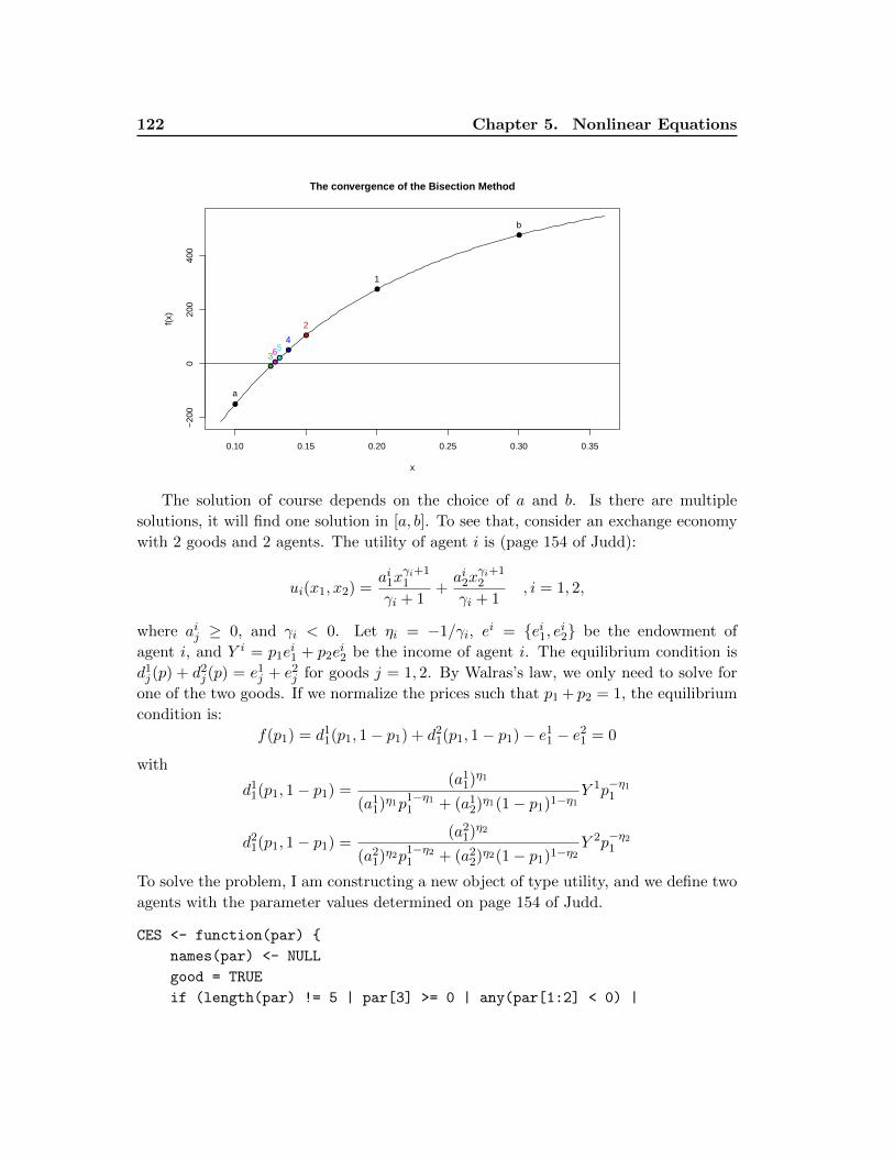
122 Chapter 5. Nonlinear Equations
0.10 0.15 0.20 0.25 0.30 0.35
−20
00
200
400
The convergence of the Bisection Method
x
f(x)
a
b
●
●
●
1
●
2
●
3●
4
●
5
●
6
The solution of course depends on the choice of a and b. Is there are multiple
solutions, it will find one solution in [a, b]. To see that, consider an exchange economy
with 2 goods and 2 agents. The utility of agent i is (page 154 of Judd):
ui(x1, x2) =ai1x
γi+11
γi + 1+ai2x
γi+12
γi + 1, i = 1, 2,
where aij ≥ 0, and γi < 0. Let ηi = −1/γi, ei = {ei1, ei2} be the endowment of
agent i, and Y i = p1ei1 + p2e
i2 be the income of agent i. The equilibrium condition is
d1j (p) + d2j (p) = e1j + e2j for goods j = 1, 2. By Walras’s law, we only need to solve for
one of the two goods. If we normalize the prices such that p1 + p2 = 1, the equilibrium
condition is:
f(p1) = d11(p1, 1− p1) + d21(p1, 1− p1)− e11 − e21 = 0
with
d11(p1, 1− p1) =(a11)
η1
(a11)η1p1−η11 + (a12)
η1(1− p1)1−η1Y 1p−η11
d21(p1, 1− p1) =(a21)
η2
(a21)η2p1−η21 + (a22)
η2(1− p1)1−η2Y 2p−η21
To solve the problem, I am constructing a new object of type utility, and we define two
agents with the parameter values determined on page 154 of Judd.
CES <- function(par) {
names(par) <- NULL
good = TRUE
if (length(par) != 5 | par[3] >= 0 | any(par[1:2] < 0) |
5.1. One-dimensional problems 123
any(par[4:5] < 0))
good <- FALSE
par <- c(a = par[1:2], gamma = par[3], eta = -1/par[3], e = par[4:5])
f <- expression(a1 * x1^(gamma + 1)/(gamma + 1) + a2 * x2^(gamma +
1)/(gamma + 1))
X1 <- expression((a1^eta/(a1^eta * p1^(1 - eta) + a2^eta *
p2^(1 - eta))) * (p1 * e1 + p2 * e2) * p1^(-eta))
X2 <- expression((a2^eta/(a1^eta * p1^(1 - eta) + a2^eta *
p2^(1 - eta))) * (p1 * e1 + p2 * e2) * p2^(-eta))
Y <- expression(e1 * p1 + e2 * p2)
Indif <- expression((((gamma + 1) * U - a1 * x1^(gamma +
1))/a2)^(1/(gamma + 1)))
fct <- paste("U = (", par[1], "*X1^", par[3] + 1, " + ",
par[2], "*X2^", par[3] + 1, "/(", par[3] + 1, sep = "")
ans <- list(Uexp = f, Sol = list(X1 = X1, X2 = X2), par = par,
name = "CES", fct = fct, Indif = Indif, good = good,
Y = Y)
class(ans) <- "Utility"
return(ans)
}
> cons1 <- consumer("John",c(1024,1,-5,12,1),utility="CES")
> cons2 <- consumer("Bill",c(1,1024,-5,1,12),utility="CES")
We can then easily compute the function that defines the equilibrium condition:
Kehoe <- function(p1) {
d1 <- sapply(1:length(p1), function(i) solve(cons1, c(p1[i],
1 - p1[i]), F)$x1)
d2 <- sapply(1:length(p1), function(i) solve(cons2, c(p1[i],
1 - p1[i]), F)$x1)
d1 + d2 - cons1$par[4] - cons2$par[4]
}
The following graph shows the shape of the excess demand function. There are three
possible equilibria.
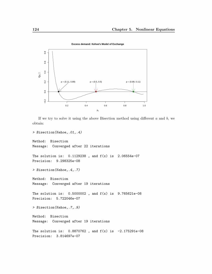
124 Chapter 5. Nonlinear Equations
0.2 0.4 0.6 0.8 1.0
−0.
20.
00.
20.
40.
60.
8Excess demand: Kehoe's Model of Exchange
p1
f(p1)
● ● ●
p = (0.11, 0.89) p = (0.5, 0.5) p = (0.89, 0.11)
If we try to solve it using the above Bisection method using different a and b, we
obtain:
> Bisection(Kehoe,.01,.4)
Method: Bisection
Message: Converged after 22 iterations
The solution is: 0.1129238 , and f(x) is 2.06554e-07
Precision: 9.298325e-08
> Bisection(Kehoe,.4,.7)
Method: Bisection
Message: Converged after 19 iterations
The solution is: 0.5000002 , and f(x) is 9.765621e-08
Precision: 5.722046e-07
> Bisection(Kehoe,.7,.9)
Method: Bisection
Message: Converged after 19 iterations
The solution is: 0.8870762 , and f(x) is -2.175291e-08
Precision: 3.814697e-07
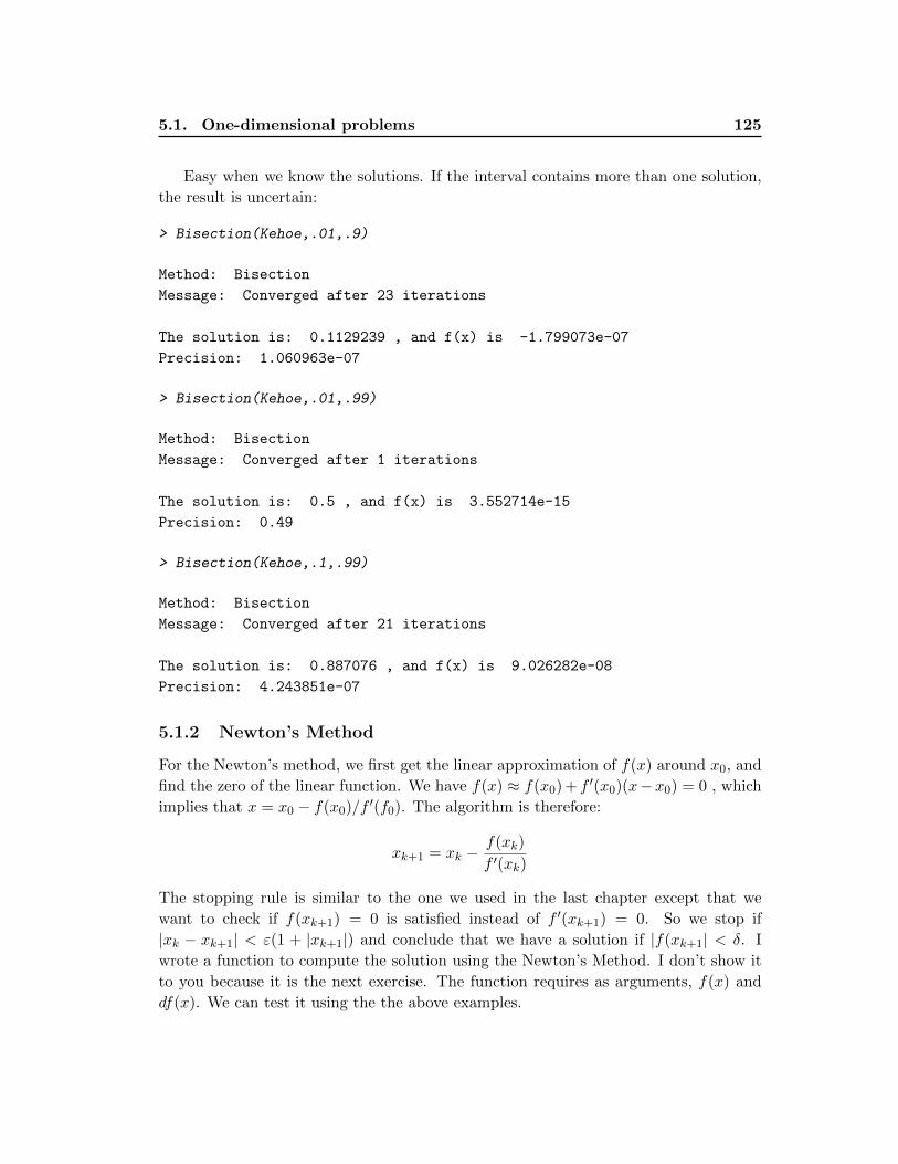
5.1. One-dimensional problems 125
Easy when we know the solutions. If the interval contains more than one solution,
the result is uncertain:
> Bisection(Kehoe,.01,.9)
Method: Bisection
Message: Converged after 23 iterations
The solution is: 0.1129239 , and f(x) is -1.799073e-07
Precision: 1.060963e-07
> Bisection(Kehoe,.01,.99)
Method: Bisection
Message: Converged after 1 iterations
The solution is: 0.5 , and f(x) is 3.552714e-15
Precision: 0.49
> Bisection(Kehoe,.1,.99)
Method: Bisection
Message: Converged after 21 iterations
The solution is: 0.887076 , and f(x) is 9.026282e-08
Precision: 4.243851e-07
5.1.2 Newton’s Method
For the Newton’s method, we first get the linear approximation of f(x) around x0, and
find the zero of the linear function. We have f(x) ≈ f(x0) + f ′(x0)(x−x0) = 0 , which
implies that x = x0 − f(x0)/f′(f0). The algorithm is therefore:
xk+1 = xk −f(xk)
f ′(xk)
The stopping rule is similar to the one we used in the last chapter except that we
want to check if f(xk+1) = 0 is satisfied instead of f ′(xk+1) = 0. So we stop if
|xk − xk+1| < ε(1 + |xk+1|) and conclude that we have a solution if |f(xk+1| < δ. I
wrote a function to compute the solution using the Newton’s Method. I don’t show it
to you because it is the next exercise. The function requires as arguments, f(x) and
df(x). We can test it using the the above examples.
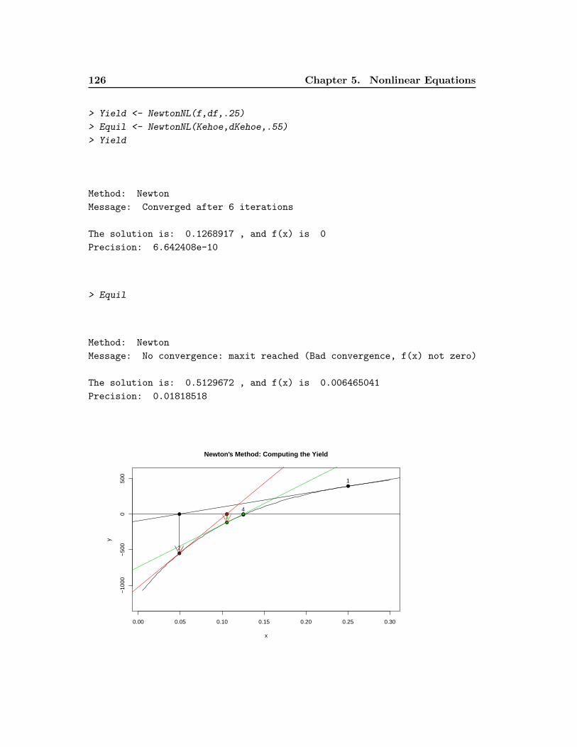
126 Chapter 5. Nonlinear Equations
> Yield <- NewtonNL(f,df,.25)
> Equil <- NewtonNL(Kehoe,dKehoe,.55)
> Yield
Method: Newton
Message: Converged after 6 iterations
The solution is: 0.1268917 , and f(x) is 0
Precision: 6.642408e-10
> Equil
Method: Newton
Message: No convergence: maxit reached (Bad convergence, f(x) not zero)
The solution is: 0.5129672 , and f(x) is 0.006465041
Precision: 0.01818518
0.00 0.05 0.10 0.15 0.20 0.25 0.30
−10
00−
500
050
0
Newton's Method: Computing the Yield
x
y
●
●
●
●
1
2
34
● ● ●
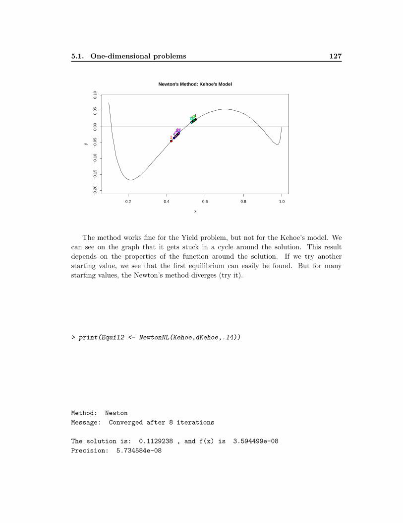
5.1. One-dimensional problems 127
0.2 0.4 0.6 0.8 1.0
−0.
20−
0.15
−0.
10−
0.05
0.00
0.05
0.10
Newton's Method: Kehoe's Model
x
y
●
●
●
●
●
●
●
●
●
●
●
●
●
●
1
2
3
4
5
6
7
8
9
10
11
12
13
14
The method works fine for the Yield problem, but not for the Kehoe’s model. We
can see on the graph that it gets stuck in a cycle around the solution. This result
depends on the properties of the function around the solution. If we try another
starting value, we see that the first equilibrium can easily be found. But for many
starting values, the Newton’s method diverges (try it).
> print(Equil2 <- NewtonNL(Kehoe,dKehoe,.14))
Method: Newton
Message: Converged after 8 iterations
The solution is: 0.1129238 , and f(x) is 3.594499e-08
Precision: 5.734584e-08
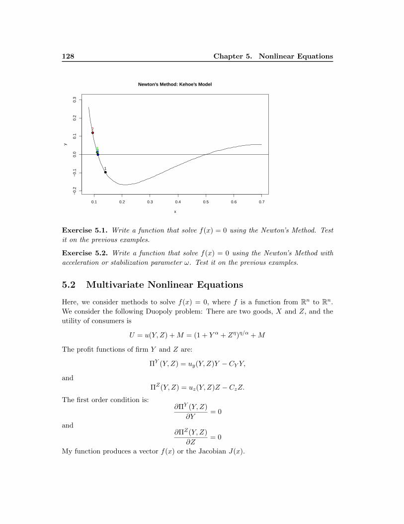
128 Chapter 5. Nonlinear Equations
0.1 0.2 0.3 0.4 0.5 0.6 0.7
−0.
2−
0.1
0.0
0.1
0.2
0.3
Newton's Method: Kehoe's Model
x
y
●
●
●●
1
2
34
Exercise 5.1. Write a function that solve f(x) = 0 using the Newton’s Method. Test
it on the previous examples.
Exercise 5.2. Write a function that solve f(x) = 0 using the Newton’s Method with
acceleration or stabilization parameter ω. Test it on the previous examples.
5.2 Multivariate Nonlinear Equations
Here, we consider methods to solve f(x) = 0, where f is a function from Rn to Rn.
We consider the following Duopoly problem: There are two goods, X and Z, and the
utility of consumers is
U = u(Y,Z) +M = (1 + Y α + Zη)η/α +M
The profit functions of firm Y and Z are:
ΠY (Y,Z) = uy(Y, Z)Y − CY Y,
and
ΠZ(Y, Z) = uz(Y, Z)Z − CzZ.
The first order condition is:∂ΠY (Y,Z)
∂Y= 0
and∂ΠZ(Y,Z)
∂Z= 0
My function produces a vector f(x) or the Jacobian J(x).
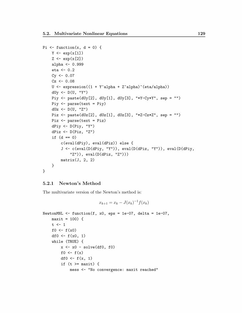
5.2. Multivariate Nonlinear Equations 129
Pi <- function(x, d = 0) {
Y <- exp(x[1])
Z <- exp(x[2])
alpha <- 0.999
eta <- 0.2
Cy <- 0.07
Cz <- 0.08
U <- expression((1 + Y^alpha + Z^alpha)^(eta/alpha))
dUy <- D(U, "Y")
Piy <- paste(dUy[2], dUy[1], dUy[3], "*Y-Cy*Y", sep = "")
Piy <- parse(text = Piy)
dUz <- D(U, "Z")
Piz <- paste(dUz[2], dUz[1], dUz[3], "*Z-Cz*Z", sep = "")
Piz <- parse(text = Piz)
dPiy <- D(Piy, "Y")
dPiz <- D(Piz, "Z")
if (d == 0)
c(eval(dPiy), eval(dPiz)) else {
J <- c(eval(D(dPiy, "Y")), eval(D(dPiz, "Y")), eval(D(dPiy,
"Z")), eval(D(dPiz, "Z")))
matrix(J, 2, 2)
}
}
5.2.1 Newton’s Method
The multivariate version of the Newton’s method is:
xk+1 = xk − J(xk)−1f(xk)
NewtonMNL <- function(f, x0, eps = 1e-07, delta = 1e-07,
maxit = 100) {
t <- 1
f0 <- f(x0)
df0 <- f(x0, 1)
while (TRUE) {
x <- x0 - solve(df0, f0)
f0 <- f(x)
df0 <- f(x, 1)
if (t >= maxit) {
mess <- "No convergence: maxit reached"
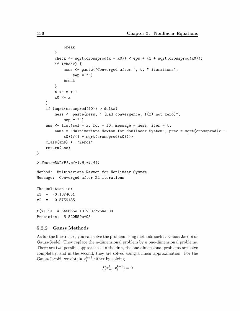
130 Chapter 5. Nonlinear Equations
break
}
check <- sqrt(crossprod(x - x0)) < eps * (1 + sqrt(crossprod(x0)))
if (check) {
mess <- paste("Converged after ", t, " iterations",
sep = "")
break
}
t <- t + 1
x0 <- x
}
if (sqrt(crossprod(f0)) > delta)
mess <- paste(mess, " (Bad convergence, f(x) not zero)",
sep = "")
ans <- list(sol = x, fct = f0, message = mess, iter = t,
name = "Multivariate Newton for Nonlinear System", prec = sqrt(crossprod(x -
x0))/(1 + sqrt(crossprod(x0))))
class(ans) <- "Zeros"
return(ans)
}
> NewtonMNL(Pi,c(-1.9,-1.4))
Method: Multivariate Newton for Nonlinear System
Message: Converged after 22 iterations
The solution is:
x1 = -0.1374651
x2 = -0.5759185
f(x) is 4.646666e-10 2.077254e-09
Precision: 5.820559e-08
5.2.2 Gauss Methods
As for the linear case, you can solve the problem using methods such as Gauss-Jacobi or
Gauss-Seidel. They replace the n-dimensional problem by n one-dimensional problems.
There are two possible approaches. In the first, the one-dimensional problems are solve
completely, and in the second, they are solved using a linear approximation. For the
Gauss-Jacobi, we obtain xk+1i either by solving
f(xk−i, xk+1i ) = 0
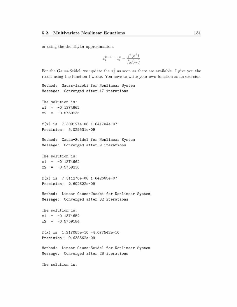
5.2. Multivariate Nonlinear Equations 131
or using the the Taylor approximation:
xk+1i = xki −
f i(xk)
f ixi(xk)
For the Gauss-Seidel, we update the xki as soon as there are available. I give you the
result using the function I wrote. You have to write your own function as an exercise.
Method: Gauss-Jacobi for Nonlinear System
Message: Converged after 17 iterations
The solution is:
x1 = -0.1374662
x2 = -0.5759235
f(x) is 7.309127e-08 1.641704e-07
Precision: 5.029531e-09
Method: Gauss-Seidel for Nonlinear System
Message: Converged after 9 iterations
The solution is:
x1 = -0.1374662
x2 = -0.5759236
f(x) is 7.311276e-08 1.642665e-07
Precision: 2.692622e-09
Method: Linear Gauss-Jacobi for Nonlinear System
Message: Converged after 32 iterations
The solution is:
x1 = -0.1374652
x2 = -0.5759184
f(x) is 1.217085e-10 -4.077542e-10
Precision: 9.638562e-09
Method: Linear Gauss-Seidel for Nonlinear System
Message: Converged after 28 iterations
The solution is:
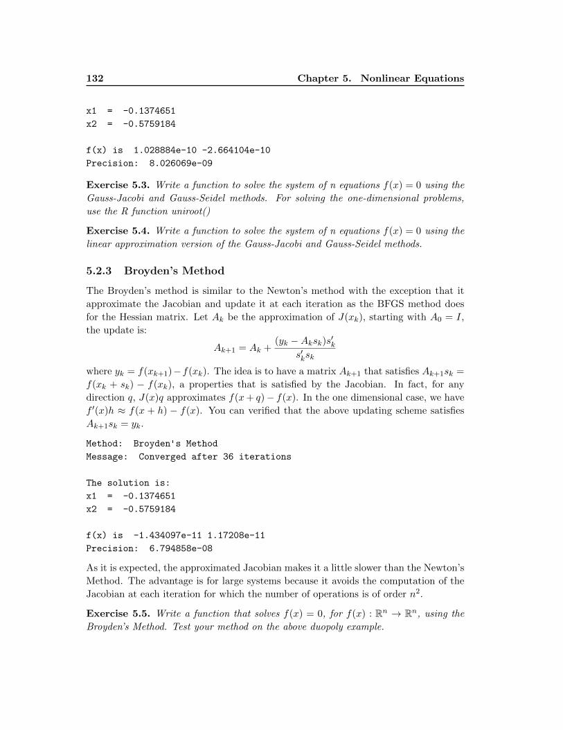
132 Chapter 5. Nonlinear Equations
x1 = -0.1374651
x2 = -0.5759184
f(x) is 1.028884e-10 -2.664104e-10
Precision: 8.026069e-09
Exercise 5.3. Write a function to solve the system of n equations f(x) = 0 using the
Gauss-Jacobi and Gauss-Seidel methods. For solving the one-dimensional problems,
use the R function uniroot()
Exercise 5.4. Write a function to solve the system of n equations f(x) = 0 using the
linear approximation version of the Gauss-Jacobi and Gauss-Seidel methods.
5.2.3 Broyden’s Method
The Broyden’s method is similar to the Newton’s method with the exception that it
approximate the Jacobian and update it at each iteration as the BFGS method does
for the Hessian matrix. Let Ak be the approximation of J(xk), starting with A0 = I,
the update is:
Ak+1 = Ak +(yk −Aksk)s′k
s′ksk
where yk = f(xk+1)−f(xk). The idea is to have a matrix Ak+1 that satisfies Ak+1sk =
f(xk + sk) − f(xk), a properties that is satisfied by the Jacobian. In fact, for any
direction q, J(x)q approximates f(x+ q)− f(x). In the one dimensional case, we have
f ′(x)h ≈ f(x + h) − f(x). You can verified that the above updating scheme satisfies
Ak+1sk = yk.
Method: Broyden's Method
Message: Converged after 36 iterations
The solution is:
x1 = -0.1374651
x2 = -0.5759184
f(x) is -1.434097e-11 1.17208e-11
Precision: 6.794858e-08
As it is expected, the approximated Jacobian makes it a little slower than the Newton’s
Method. The advantage is for large systems because it avoids the computation of the
Jacobian at each iteration for which the number of operations is of order n2.
Exercise 5.5. Write a function that solves f(x) = 0, for f(x) : Rn → Rn, using the
Broyden’s Method. Test your method on the above duopoly example.
5.2. Multivariate Nonlinear Equations 133
5.2.4 The nleqslv package
The nleqslv package of [Hasselman 2012] provides functions for solving systems of non-
linear equations. The main function is nleqslv() which uses either the Newton or the
Broyden’s method. The function uses a method similar to the one we saw in the last
chapter for improving the convergence speed. The updating scheme is xk+1 = xk+λsk.
The lambda is selected using a kind of line search. The criterion is base on the impact
of the step on f(x)′f(x). The options are:
� The first three are respectively x0, f and J , where f and J are functions.
� method = either ”Broyden” of ”Newton”
� global = different method for selecting the λ. You can choose ”none” if you want
λ = 1
� xscalm = method for re-scaling the x’s. You always make sure the xi’s have
comparable scales.
� control = list(): Many parameter to adjust if you want. For example, xtol and ftol
are what we call ε and δ in the above algorithms, maxit the number of iterations,
trace=1 will print the details of each iterations, and a bunch of other tuning
parameters.
To see how it works, we apply it to the duopoly problem.
> library(nleqslv)
> dPi <- function(x)
+ Pi(x,1)
> nleqslv(c(-1,-2),Pi,dPi)
$x
[1] -0.1374651 -0.5759186
$fvec
[1] -1.782566e-09 3.254971e-09
$termcd
[1] 1
$message
[1] "Function criterion near zero"
$scalex
134 Chapter 5. Nonlinear Equations
[1] 1 1
$nfcnt
[1] 15
$njcnt
[1] 1
See the help() to understand all code. In particular we see that there is only one
Jacobian evaluation (because it is the Broyden’s Method) and 15 function evaluations.
5.2.5 Example
Consider the endowment economy in which there are m goods, and n agents with
utilities:
ui(x) =
m∑j=1
aijxvij+1j
1 + vij, i = 1, ..., n,
endowed with eij units of good j, where m = n = 10, and the coefficients are obtained
randomly as follows (for a, e and v, the ith row is for the ith agent and the jth column
the jth good):
> set.seed(445)
> n <- 10
> m <- 10
> a <- matrix(runif(n*m,1,10),n,m)
> v <- matrix(runif(n*m,-3,-0.5),n,m)
> e <- matrix(runif(n*m,1,5),n,m)
By using Walras law and the normalization∑m
i=1 pi = 1, the problem is to solve the
following equations:
E1(p) =0
E2(p) =0
...
Em−1(p) =0m∑i=1
pi =1,
where Ei(p) is the excess demand of good i.

5.2. Multivariate Nonlinear Equations 135
Exercise 5.6. Solve the equilibrium problem of the above endowment economy. Use
the algorithm that you want but Ei(p) must be obtained numerically using the optimizer
of your choice.

Chapter 6
Numerical Calculus
Contents
6.1 Numerical Integration . . . . . . . . . . . . . . . . . . . . . . . . . 137
6.1.1 Newton-Cotes . . . . . . . . . . . . . . . . . . . . . . . . . . . . . . 138
6.1.2 Gauss Methods . . . . . . . . . . . . . . . . . . . . . . . . . . . . . 142
6.1.3 Numerical integration with R . . . . . . . . . . . . . . . . . . . . . 146
6.1.4 Numerical derivatives with R . . . . . . . . . . . . . . . . . . . . . 147
6.1 Numerical Integration
We introduce the section with two examples. In the first, we consider the following
portfolio optimization problem:
maxωi
E
[U
(n∑i=1
ωiZi
)](6.1)
subject ton∑i=1
pi(ωi − ei) = 0 (6.2)
It may look like a simple maximization problem, but it is not. The difficulty comes
from the fact that we have to maximize an expected value, which can be written as:
E
[U
(n∑i=1
ωiZi
)]=
∫ ∫· · ·∫U
(n∑i=1
ωiZi
)f(Z1, Z2, ..., Zn)dZ1dZ2 · · · dZn
In the basic model, we assume that the preferences are mean-variance, an assumption
that can be satisfied if either U() is quadratic or the vector Z is characterized by
an elliptical distribution. In that case. only the mean and the variance matter, and
the investors choose a combination of the risk free asset and the market portfolio. It
simplifies the problem, but does not eliminate the need to compute integrals. For
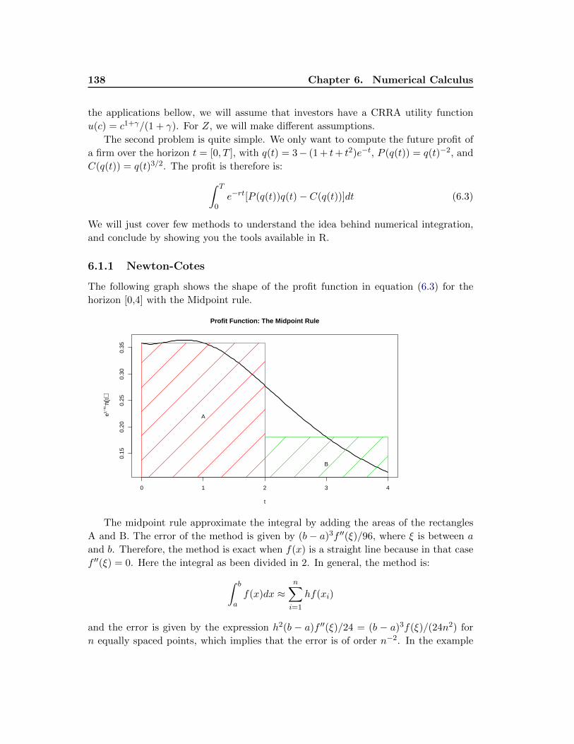
138 Chapter 6. Numerical Calculus
the applications bellow, we will assume that investors have a CRRA utility function
u(c) = c1+γ/(1 + γ). For Z, we will make different assumptions.
The second problem is quite simple. We only want to compute the future profit of
a firm over the horizon t = [0, T ], with q(t) = 3− (1 + t+ t2)e−t, P (q(t)) = q(t)−2, and
C(q(t)) = q(t)3/2. The profit is therefore is:∫ T
0e−rt[P (q(t))q(t)− C(q(t))]dt (6.3)
We will just cover few methods to understand the idea behind numerical integration,
and conclude by showing you the tools available in R.
6.1.1 Newton-Cotes
The following graph shows the shape of the profit function in equation (6.3) for the
horizon [0,4] with the Midpoint rule.
0 1 2 3 4
0.15
0.20
0.25
0.30
0.35
Profit Function: The Midpoint Rule
t
e(−rt) π(
t)
A
B
The midpoint rule approximate the integral by adding the areas of the rectangles
A and B. The error of the method is given by (b − a)3f ′′(ξ)/96, where ξ is between a
and b. Therefore, the method is exact when f(x) is a straight line because in that case
f ′′(ξ) = 0. Here the integral as been divided in 2. In general, the method is:∫ b
af(x)dx ≈
n∑i=1
hf(xi)
and the error is given by the expression h2(b − a)f ′′(ξ)/24 = (b − a)3f(ξ)/(24n2) for
n equally spaced points, which implies that the error is of order n−2. In the example
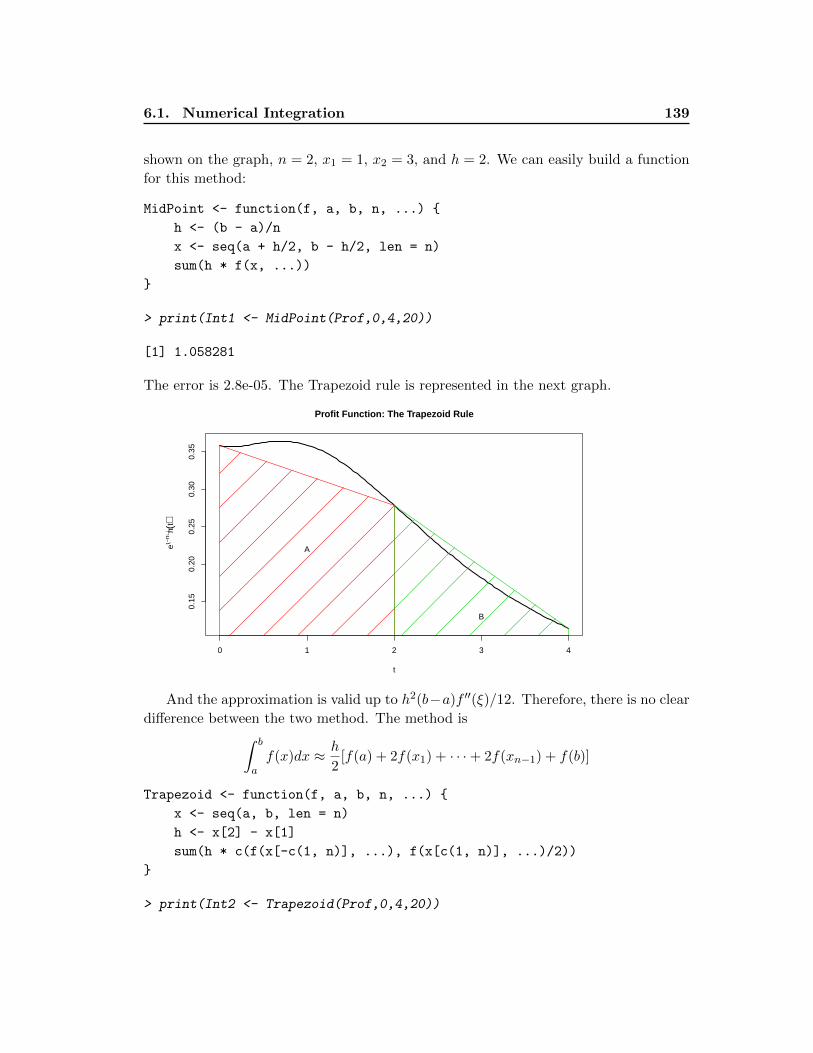
6.1. Numerical Integration 139
shown on the graph, n = 2, x1 = 1, x2 = 3, and h = 2. We can easily build a function
for this method:
MidPoint <- function(f, a, b, n, ...) {
h <- (b - a)/n
x <- seq(a + h/2, b - h/2, len = n)
sum(h * f(x, ...))
}
> print(Int1 <- MidPoint(Prof,0,4,20))
[1] 1.058281
The error is 2.8e-05. The Trapezoid rule is represented in the next graph.
0 1 2 3 4
0.15
0.20
0.25
0.30
0.35
Profit Function: The Trapezoid Rule
t
e(−rt) π(
t)
A
B
And the approximation is valid up to h2(b−a)f ′′(ξ)/12. Therefore, there is no clear
difference between the two method. The method is∫ b
af(x)dx ≈ h
2[f(a) + 2f(x1) + · · ·+ 2f(xn−1) + f(b)]
Trapezoid <- function(f, a, b, n, ...) {
x <- seq(a, b, len = n)
h <- x[2] - x[1]
sum(h * c(f(x[-c(1, n)], ...), f(x[c(1, n)], ...)/2))
}
> print(Int2 <- Trapezoid(Prof,0,4,20))
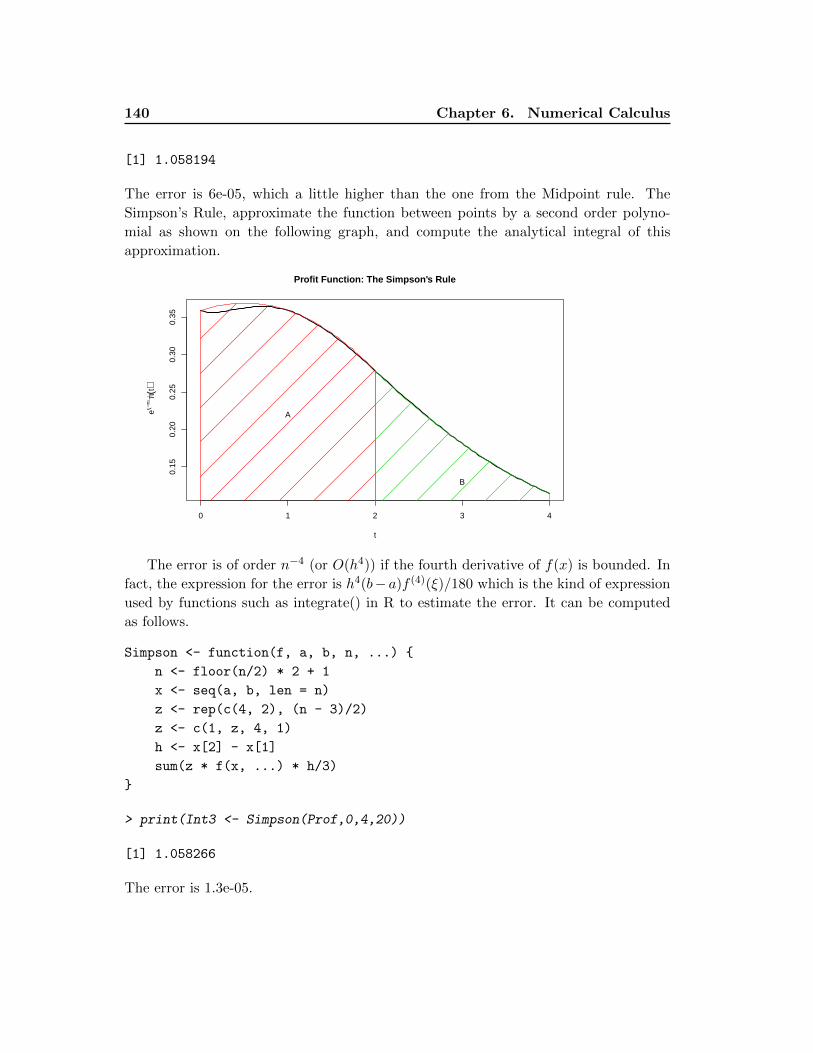
140 Chapter 6. Numerical Calculus
[1] 1.058194
The error is 6e-05, which a little higher than the one from the Midpoint rule. The
Simpson’s Rule, approximate the function between points by a second order polyno-
mial as shown on the following graph, and compute the analytical integral of this
approximation.
0 1 2 3 4
0.15
0.20
0.25
0.30
0.35
Profit Function: The Simpson's Rule
t
e(−rt) π(
t)
A
B
The error is of order n−4 (or O(h4)) if the fourth derivative of f(x) is bounded. In
fact, the expression for the error is h4(b− a)f (4)(ξ)/180 which is the kind of expression
used by functions such as integrate() in R to estimate the error. It can be computed
as follows.
Simpson <- function(f, a, b, n, ...) {
n <- floor(n/2) * 2 + 1
x <- seq(a, b, len = n)
z <- rep(c(4, 2), (n - 3)/2)
z <- c(1, z, 4, 1)
h <- x[2] - x[1]
sum(z * f(x, ...) * h/3)
}
> print(Int3 <- Simpson(Prof,0,4,20))
[1] 1.058266
The error is 1.3e-05.
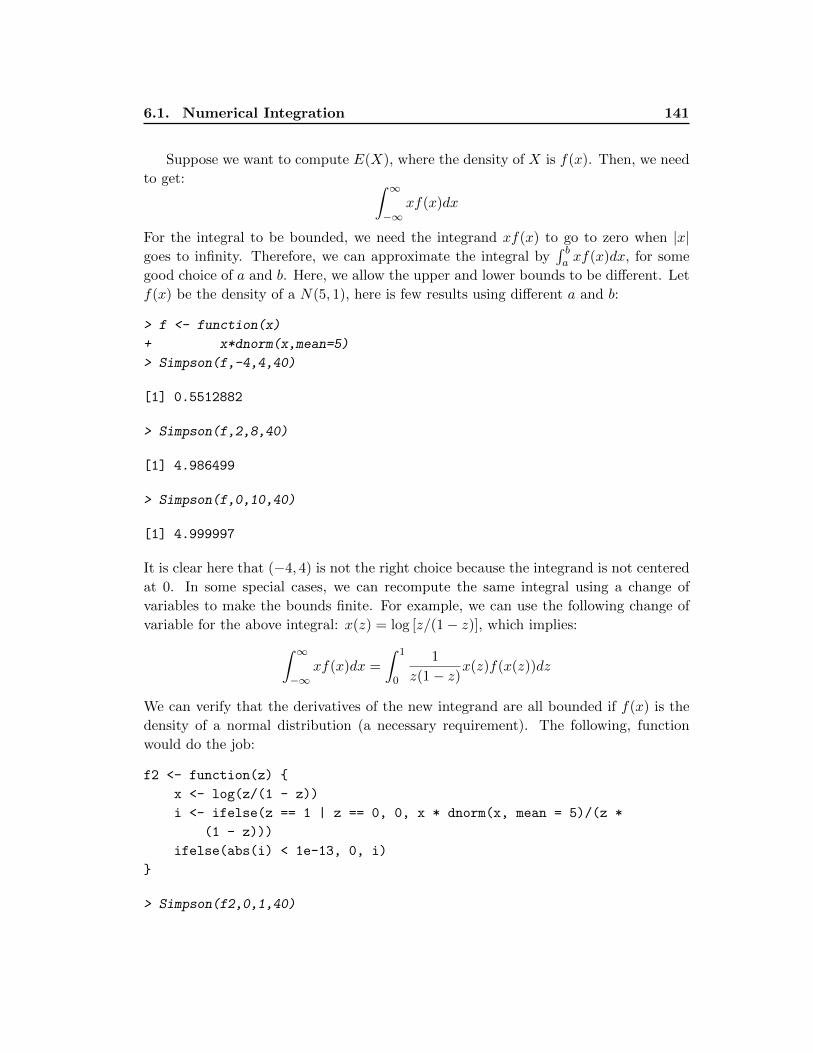
6.1. Numerical Integration 141
Suppose we want to compute E(X), where the density of X is f(x). Then, we need
to get: ∫ ∞−∞
xf(x)dx
For the integral to be bounded, we need the integrand xf(x) to go to zero when |x|goes to infinity. Therefore, we can approximate the integral by
∫ ba xf(x)dx, for some
good choice of a and b. Here, we allow the upper and lower bounds to be different. Let
f(x) be the density of a N(5, 1), here is few results using different a and b:
> f <- function(x)
+ x*dnorm(x,mean=5)
> Simpson(f,-4,4,40)
[1] 0.5512882
> Simpson(f,2,8,40)
[1] 4.986499
> Simpson(f,0,10,40)
[1] 4.999997
It is clear here that (−4, 4) is not the right choice because the integrand is not centered
at 0. In some special cases, we can recompute the same integral using a change of
variables to make the bounds finite. For example, we can use the following change of
variable for the above integral: x(z) = log [z/(1− z)], which implies:∫ ∞−∞
xf(x)dx =
∫ 1
0
1
z(1− z)x(z)f(x(z))dz
We can verify that the derivatives of the new integrand are all bounded if f(x) is the
density of a normal distribution (a necessary requirement). The following, function
would do the job:
f2 <- function(z) {
x <- log(z/(1 - z))
i <- ifelse(z == 1 | z == 0, 0, x * dnorm(x, mean = 5)/(z *
(1 - z)))
ifelse(abs(i) < 1e-13, 0, i)
}
> Simpson(f2,0,1,40)
142 Chapter 6. Numerical Calculus
[1] 0.896398
The result is not very good. The problem here is that the function is close to zero
almost everywhere except between 0.9 and 1, as we can see on the following graph:
0.95 0.96 0.97 0.98 0.99 1.00
010
020
030
040
050
060
0
Integrand of E(x), where X is N(5,1)
x
f2(x
) log(z (1 − z))z(1 − z) 2π
exp(− 0.5(x(z) − 5)2)
We need more points when the slope of the function changes quickly. We also want
to avoid adding values that are dominated by rounding errors:
> Simpson(f2,0.8,1,1000)
[1] 4.999595
6.1.2 Gauss Methods
The Gauss approach is to approximate the function using orthogonal basis, and to
choose optimal weights and nodes simultaneously. In fact, the nodes and weights are
such that ∫ b
af(x)w(x)dx =
n∑i=1
ωif(xi)
holds exactly for all polynomial of degree 2n− 1, f(x). The integrating function w(x)
defines the inner product < f, g > so that the basis used to approximate f(x) are
orthogonal and standardized with respect to this inner product (see Chapter 6 of Judd
for more details). The different sets of basis are given in Table 6.3, page 204, of Judd.
There is an optimal quadrature for each w(x), but we can also do a change of variable
when w(x) is missing. For example, the Gauss-Chebyshev, w(x) = (1− x2)−1/2, and it
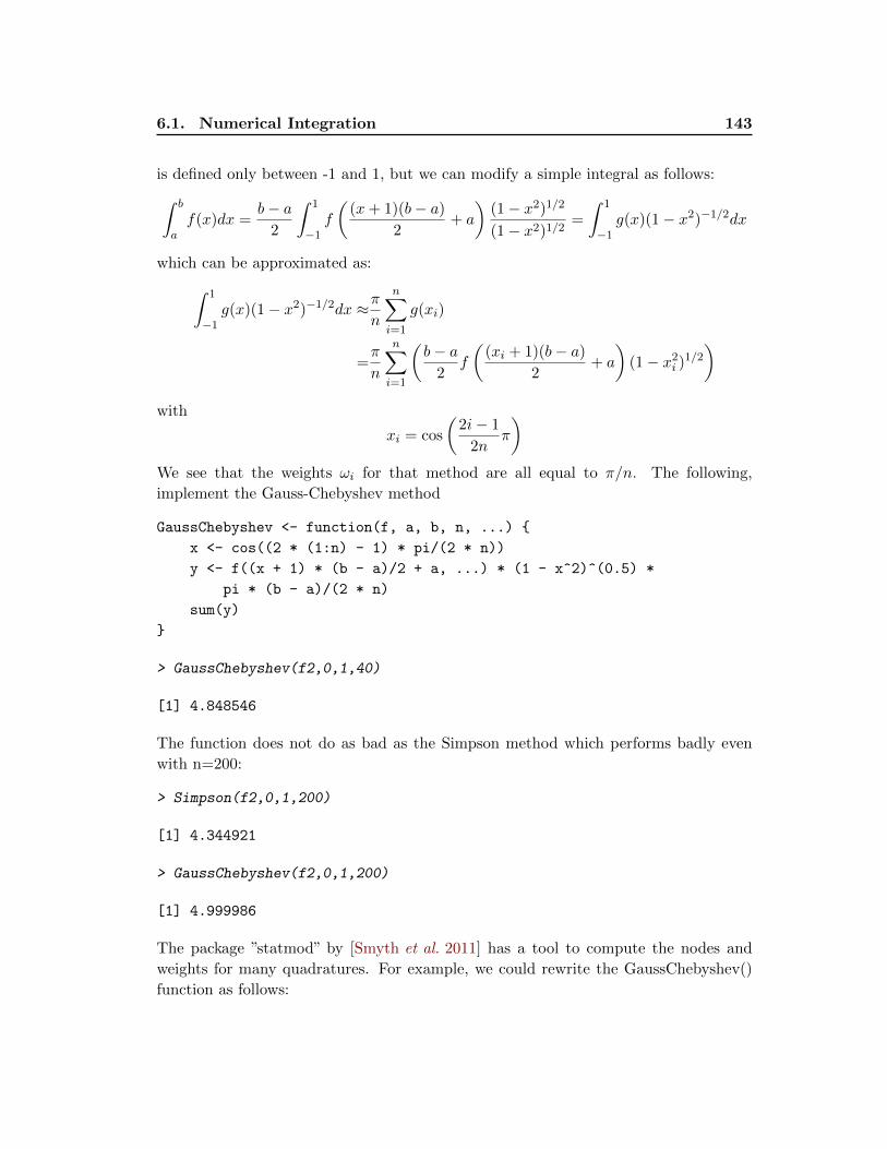
6.1. Numerical Integration 143
is defined only between -1 and 1, but we can modify a simple integral as follows:∫ b
af(x)dx =
b− a2
∫ 1
−1f
((x+ 1)(b− a)
2+ a
)(1− x2)1/2
(1− x2)1/2=
∫ 1
−1g(x)(1− x2)−1/2dx
which can be approximated as:∫ 1
−1g(x)(1− x2)−1/2dx ≈π
n
n∑i=1
g(xi)
=π
n
n∑i=1
(b− a
2f
((xi + 1)(b− a)
2+ a
)(1− x2i )1/2
)with
xi = cos
(2i− 1
2nπ
)We see that the weights ωi for that method are all equal to π/n. The following,
implement the Gauss-Chebyshev method
GaussChebyshev <- function(f, a, b, n, ...) {
x <- cos((2 * (1:n) - 1) * pi/(2 * n))
y <- f((x + 1) * (b - a)/2 + a, ...) * (1 - x^2)^(0.5) *
pi * (b - a)/(2 * n)
sum(y)
}
> GaussChebyshev(f2,0,1,40)
[1] 4.848546
The function does not do as bad as the Simpson method which performs badly even
with n=200:
> Simpson(f2,0,1,200)
[1] 4.344921
> GaussChebyshev(f2,0,1,200)
[1] 4.999986
The package ”statmod” by [Smyth et al. 2011] has a tool to compute the nodes and
weights for many quadratures. For example, we could rewrite the GaussChebyshev()
function as follows:
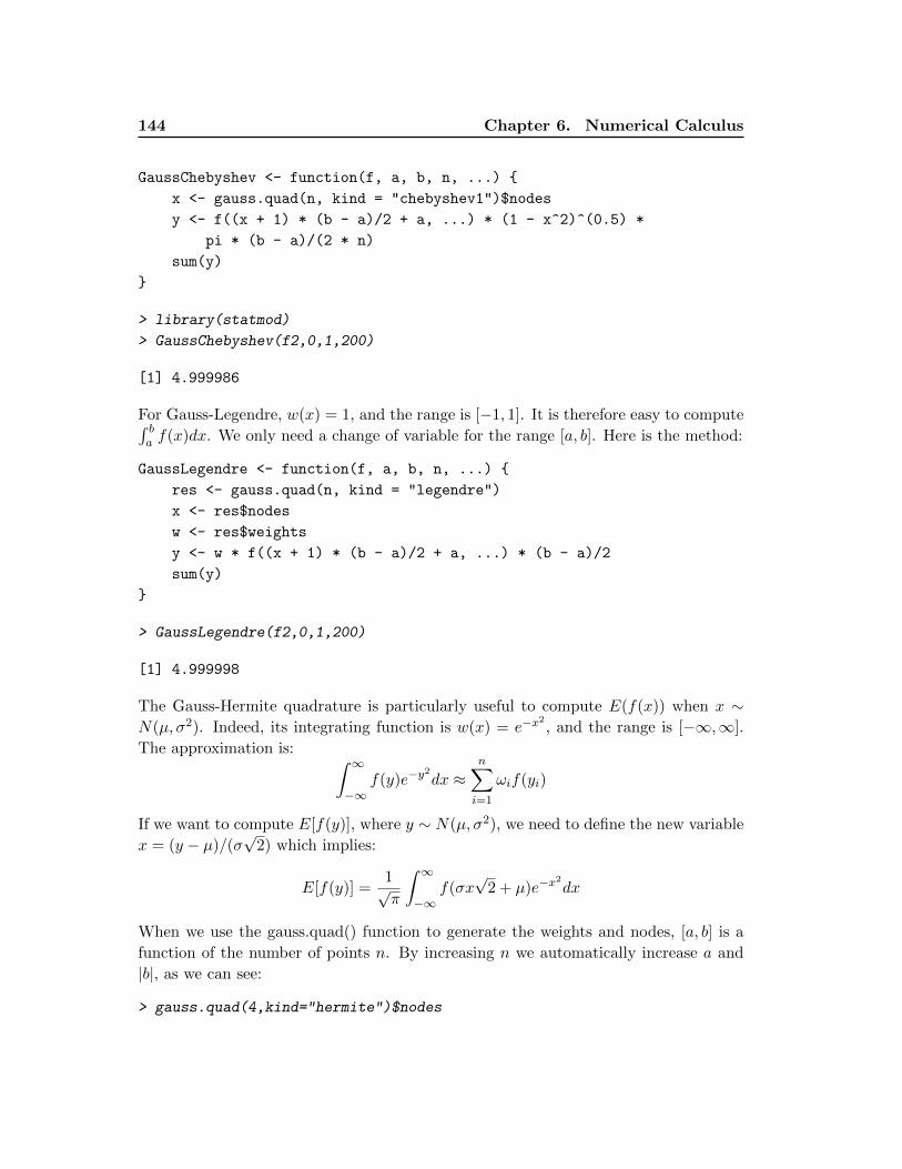
144 Chapter 6. Numerical Calculus
GaussChebyshev <- function(f, a, b, n, ...) {
x <- gauss.quad(n, kind = "chebyshev1")$nodes
y <- f((x + 1) * (b - a)/2 + a, ...) * (1 - x^2)^(0.5) *
pi * (b - a)/(2 * n)
sum(y)
}
> library(statmod)
> GaussChebyshev(f2,0,1,200)
[1] 4.999986
For Gauss-Legendre, w(x) = 1, and the range is [−1, 1]. It is therefore easy to compute∫ ba f(x)dx. We only need a change of variable for the range [a, b]. Here is the method:
GaussLegendre <- function(f, a, b, n, ...) {
res <- gauss.quad(n, kind = "legendre")
x <- res$nodes
w <- res$weights
y <- w * f((x + 1) * (b - a)/2 + a, ...) * (b - a)/2
sum(y)
}
> GaussLegendre(f2,0,1,200)
[1] 4.999998
The Gauss-Hermite quadrature is particularly useful to compute E(f(x)) when x ∼N(µ, σ2). Indeed, its integrating function is w(x) = e−x
2, and the range is [−∞,∞].
The approximation is: ∫ ∞−∞
f(y)e−y2dx ≈
n∑i=1
ωif(yi)
If we want to compute E[f(y)], where y ∼ N(µ, σ2), we need to define the new variable
x = (y − µ)/(σ√
2) which implies:
E[f(y)] =1√π
∫ ∞−∞
f(σx√
2 + µ)e−x2dx
When we use the gauss.quad() function to generate the weights and nodes, [a, b] is a
function of the number of points n. By increasing n we automatically increase a and
|b|, as we can see:
> gauss.quad(4,kind="hermite")$nodes
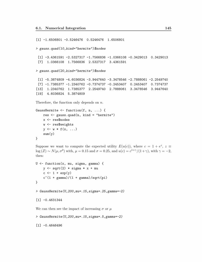
6.1. Numerical Integration 145
[1] -1.6506801 -0.5246476 0.5246476 1.6506801
> gauss.quad(10,kind="hermite")$nodes
[1] -3.4361591 -2.5327317 -1.7566836 -1.0366108 -0.3429013 0.3429013
[7] 1.0366108 1.7566836 2.5327317 3.4361591
> gauss.quad(20,kind="hermite")$nodes
[1] -5.3874809 -4.6036824 -3.9447640 -3.3478546 -2.7888061 -2.2549740
[7] -1.7385377 -1.2340762 -0.7374737 -0.2453407 0.2453407 0.7374737
[13] 1.2340762 1.7385377 2.2549740 2.7888061 3.3478546 3.9447640
[19] 4.6036824 5.3874809
Therefore, the function only depends on n.
GaussHermite <- function(f, n, ...) {
res <- gauss.quad(n, kind = "hermite")
x <- res$nodes
w <- res$weights
y <- w * f(x, ...)
sum(y)
}
Suppose we want to compute the expected utility E(u(c)), where c = 1 + ez, z ≡log (Z) ∼ N(µ, σ2) with, µ = 0.15 and σ = 0.25, and u(c) = c1+γ/(1+γ), with γ = −2,
then:
U <- function(x, mu, sigma, gamma) {
y <- sqrt(2) * sigma * x + mu
c <- 1 + exp(y)
c^(1 + gamma)/(1 + gamma)/sqrt(pi)
}
> GaussHermite(U,200,mu=.15,sigma=.25,gamma=-2)
[1] -0.4631344
We can then see the impact of increasing σ or µ
> GaussHermite(U,200,mu=.15,sigma=.5,gamma=-2)
[1] -0.4646496
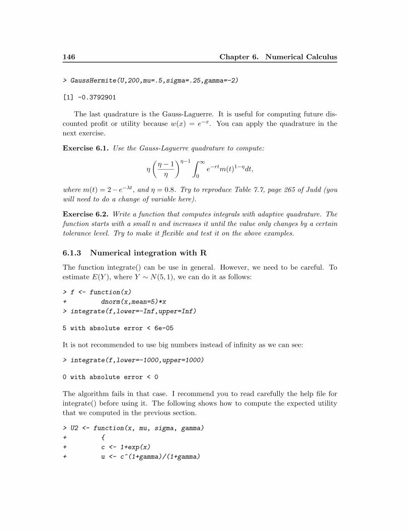
146 Chapter 6. Numerical Calculus
> GaussHermite(U,200,mu=.5,sigma=.25,gamma=-2)
[1] -0.3792901
The last quadrature is the Gauss-Laguerre. It is useful for computing future dis-
counted profit or utility because w(x) = e−x. You can apply the quadrature in the
next exercise.
Exercise 6.1. Use the Gauss-Laguerre quadrature to compute:
η
(η − 1
η
)η−1 ∫ ∞0
e−rtm(t)1−ηdt,
where m(t) = 2− e−λt, and η = 0.8. Try to reproduce Table 7.7, page 265 of Judd (you
will need to do a change of variable here).
Exercise 6.2. Write a function that computes integrals with adaptive quadrature. The
function starts with a small n and increases it until the value only changes by a certain
tolerance level. Try to make it flexible and test it on the above examples.
6.1.3 Numerical integration with R
The function integrate() can be use in general. However, we need to be careful. To
estimate E(Y ), where Y ∼ N(5, 1), we can do it as follows:
> f <- function(x)
+ dnorm(x,mean=5)*x
> integrate(f,lower=-Inf,upper=Inf)
5 with absolute error < 6e-05
It is not recommended to use big numbers instead of infinity as we can see:
> integrate(f,lower=-1000,upper=1000)
0 with absolute error < 0
The algorithm fails in that case. I recommend you to read carefully the help file for
integrate() before using it. The following shows how to compute the expected utility
that we computed in the previous section.
> U2 <- function(x, mu, sigma, gamma)
+ {
+ c <- 1+exp(x)
+ u <- c^(1+gamma)/(1+gamma)
6.1. Numerical Integration 147
+ u*dnorm(x,mean=mu,sd=sigma)
+ }
> f <- function(x)
+ U2(x,.15,.25,-2)
> integrate(f,-Inf,Inf)
-0.4631344 with absolute error < 0.00011
Exercise 6.3. In a statistical method called the Generalized Empirical Likelihood for
a continuum, we need to compute an n× n matrix C with
cij =
∫ ∞−∞
e−(xi−xj)2t2φ(t)dt,
where φ(t) is the density of the standardized normal distribution, and xi is observation
i. Find a fast way to construct that matrix, and test your method with the 2000 × 1
vector x generated from a N(10, 2).
6.1.4 Numerical derivatives with R
Here is how to do numerical derivative in R. The following is taken from
help(numericDeriv) file.
> myenv <- new.env()
> assign("mean", 0., envir = myenv)
> assign("sd", 1., envir = myenv)
> assign("x", c(-2,0,2), envir = myenv)
> grad <- numericDeriv(quote(pnorm(x, mean, sd)), c("mean", "sd"), myenv)
> attr(grad,"gradient")
[,1] [,2]
[1,] -0.05399097 0.1079819
[2,] -0.39894228 0.0000000
[3,] -0.05399097 -0.1079819
Exercise 6.4. Write a function df(f,x) and ddf(f,x) that return the Jacobian and Hes-
sian of f(x) : Rn → R, using numericDeriv().

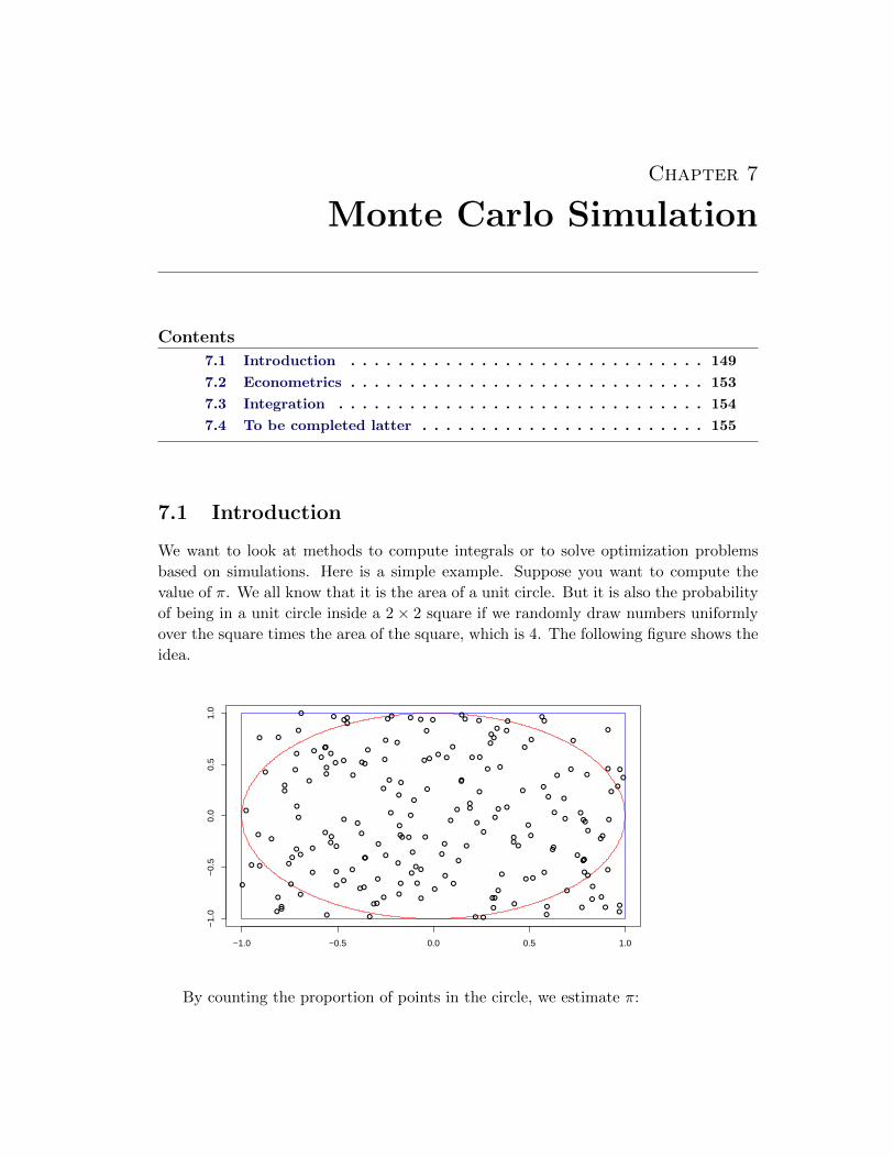
Chapter 7
Monte Carlo Simulation
Contents
7.1 Introduction . . . . . . . . . . . . . . . . . . . . . . . . . . . . . . 149
7.2 Econometrics . . . . . . . . . . . . . . . . . . . . . . . . . . . . . . 153
7.3 Integration . . . . . . . . . . . . . . . . . . . . . . . . . . . . . . . 154
7.4 To be completed latter . . . . . . . . . . . . . . . . . . . . . . . . 155
7.1 Introduction
We want to look at methods to compute integrals or to solve optimization problems
based on simulations. Here is a simple example. Suppose you want to compute the
value of π. We all know that it is the area of a unit circle. But it is also the probability
of being in a unit circle inside a 2× 2 square if we randomly draw numbers uniformly
over the square times the area of the square, which is 4. The following figure shows the
idea.
−1.0 −0.5 0.0 0.5 1.0
−1.
0−
0.5
0.0
0.5
1.0
●
●
●
●
●
●
●
●
●●
●
●
●
●
●
●
●
●
●
●
●
●
●
●
●
●
●
●
●
●
●
●
●
●
●
●
●
●
●
●
●
●
●
●
●
●
●
●●
●
●
●
●
●
●
●
●
●
●
●
●
●
●
●
●
●
●●
●
●
●
●
●
●
●
●
●
●
●
●
●
●
●
●
●
●
●
●
●
●
●
●●
●
●
●
●
● ●
●●
●
●
●
●
●
●
●
●
●
●
●
●
●
●
●
●
●
●
● ●
●
●
●
●
●
●
●
●
●
●
●
●
●
●
●
●
● ●
●
●
●
●
●
●
●
●
●
●
●
●
●
●
●
●
●
●
●
●
●
●
●
●
●
●
●
●
●
●
●
●
●
●
●
●
●
●
●
●
●
●
●
●
●
●
●
●
●
●
●
●
●
●
●
●
●●
●●
●
By counting the proportion of points in the circle, we estimate π:
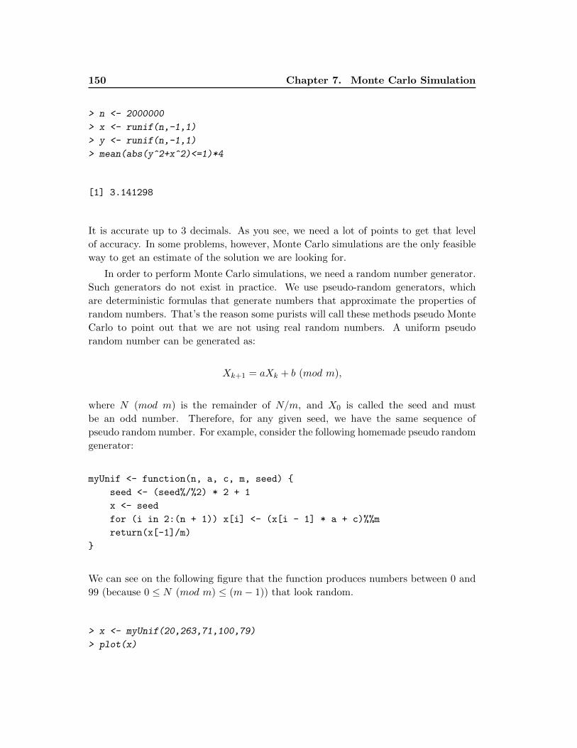
150 Chapter 7. Monte Carlo Simulation
> n <- 2000000
> x <- runif(n,-1,1)
> y <- runif(n,-1,1)
> mean(abs(y^2+x^2)<=1)*4
[1] 3.141298
It is accurate up to 3 decimals. As you see, we need a lot of points to get that level
of accuracy. In some problems, however, Monte Carlo simulations are the only feasible
way to get an estimate of the solution we are looking for.
In order to perform Monte Carlo simulations, we need a random number generator.
Such generators do not exist in practice. We use pseudo-random generators, which
are deterministic formulas that generate numbers that approximate the properties of
random numbers. That’s the reason some purists will call these methods pseudo Monte
Carlo to point out that we are not using real random numbers. A uniform pseudo
random number can be generated as:
Xk+1 = aXk + b (mod m),
where N (mod m) is the remainder of N/m, and X0 is called the seed and must
be an odd number. Therefore, for any given seed, we have the same sequence of
pseudo random number. For example, consider the following homemade pseudo random
generator:
myUnif <- function(n, a, c, m, seed) {
seed <- (seed%/%2) * 2 + 1
x <- seed
for (i in 2:(n + 1)) x[i] <- (x[i - 1] * a + c)%%m
return(x[-1]/m)
}
We can see on the following figure that the function produces numbers between 0 and
99 (because 0 ≤ N (mod m) ≤ (m− 1)) that look random.
> x <- myUnif(20,263,71,100,79)
> plot(x)
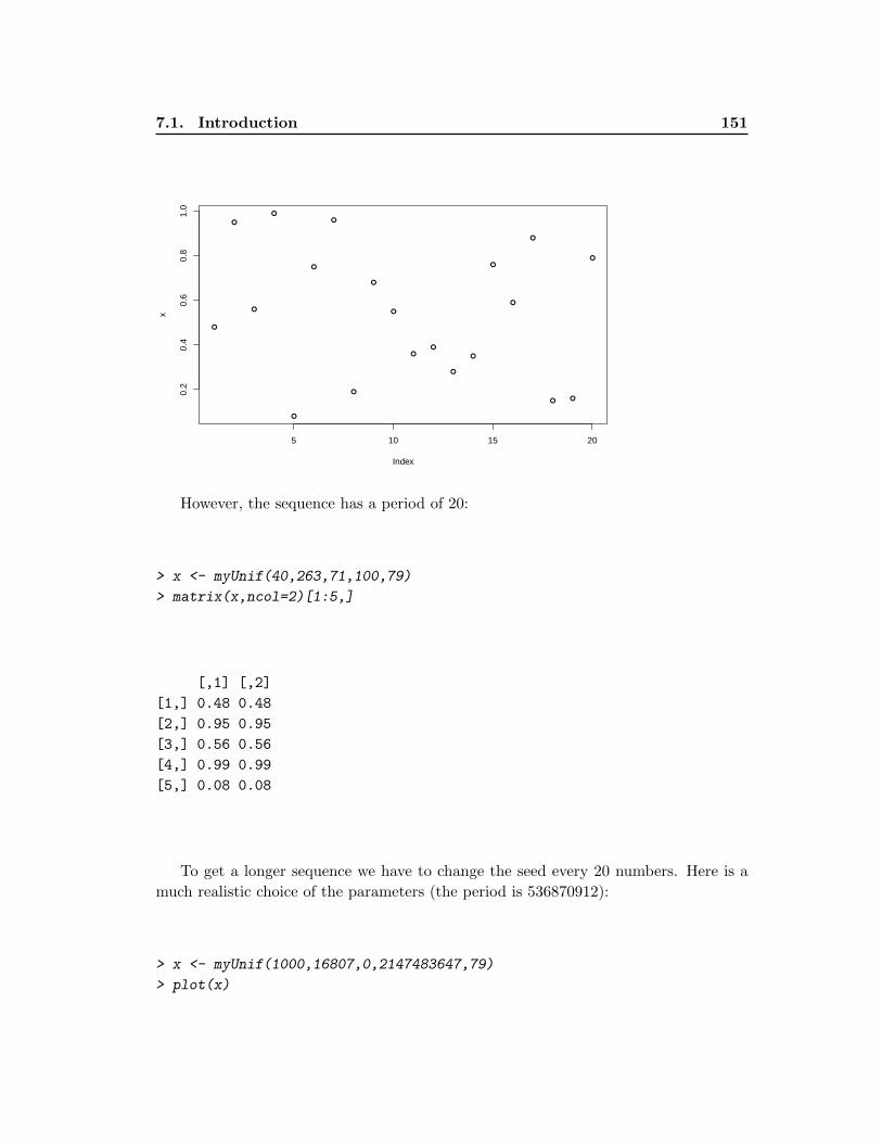
7.1. Introduction 151
●
●
●
●
●
●
●
●
●
●
●
●
●
●
●
●
●
● ●
●
5 10 15 20
0.2
0.4
0.6
0.8
1.0
Index
x
However, the sequence has a period of 20:
> x <- myUnif(40,263,71,100,79)
> matrix(x,ncol=2)[1:5,]
[,1] [,2]
[1,] 0.48 0.48
[2,] 0.95 0.95
[3,] 0.56 0.56
[4,] 0.99 0.99
[5,] 0.08 0.08
To get a longer sequence we have to change the seed every 20 numbers. Here is a
much realistic choice of the parameters (the period is 536870912):
> x <- myUnif(1000,16807,0,2147483647,79)
> plot(x)
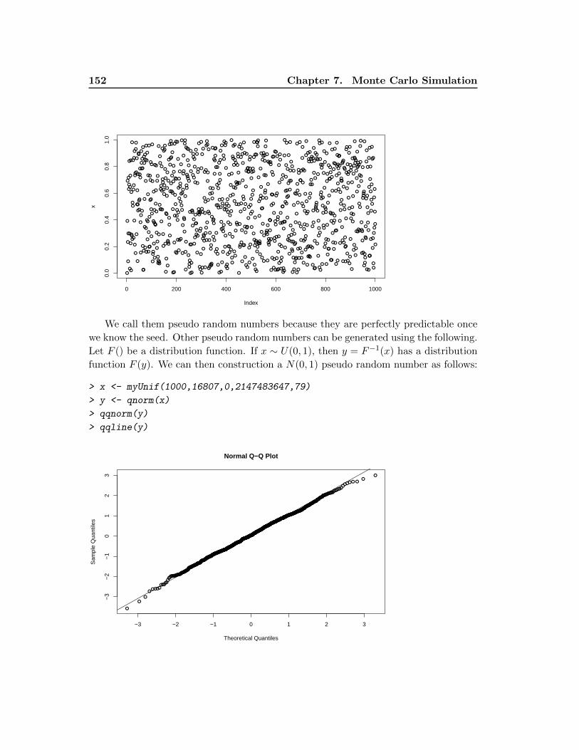
152 Chapter 7. Monte Carlo Simulation
●
●
●
●
●
●
●
●
●
●
●
●
●
●
●
●
●
●
●●
●
●
●●
●
●
●
●
●
●
●
●
●●
●
●
●
●
●
●
●
●
●
●
●
●
●●
●
●
●
●
●
●
●
●
●
●
●
●
●
●
●
●
●
●●
●
●
●
●
●
●
●
●
●
●
●
●
●
●
●
●
●
●
●
●
●
●
●
●
●
●
●
●
●
●
●
●
●
●
●
●
●
●●
●
●
●
●
●
●
●
●●
●
●
●
●
●
●
●
●
●
●
●●
●
●
●●
●
●
●
●
●
●
●
●
●
●
●
●
●●
●
●
●
●
●
●
●●
●
●
●
●
●
●
●
●
●
●
●
●●
●
●
●
●
●
●
●
●
●
●
●
●
●
●
●
●
●
●
●
●
●
●
●
●
●
●
●
●
●
●
●
●
●
●
●
●
●
●
●
●
●
●
●
●
●
●
●
●●
●
●
●
●
●
●
●
●
●
●
●
●
●
●
●●
●
●●
●
●
●
●
●
●●
●
●
●
●
●
●
●
●
●
●●●
●
●
●
●
●
●
●
●
●●●
●
●
●●
●
●
●
●
●
●
●
●
●
●
●
●
●
●
●
●
●
●●
●●
●
●●
●
●
●
●
●
●
●
●
●
●
●
●
●
●
●
●
●●
●
●
●
●
●
●
●
●
●
●
●
●
●
●
●
●
●
●
●
●
●
●
●
●
●
●
●
●●
●●
●
●
●
●
●
●
●
●●
●
●
●
●
●
●
●
●
●
●
●
●
●
●
●
●
●
●
●
●
●
●
●
●
●
●
●
●
●
●
●
●
●
●●
●
●
●
●
●
●
●
●●
●
●
●
●
●
●
●
●
●●
●
●
●
●
●
●
●
●
●
●
●
●
●
●
●
●
●
●
●
●
●
●
●
●
●
●
●
●
●
●
●
●
●
●
●
●
●
●
●
●
●
●
●●
●
●
●
●
●
●
●●
●
●
●
●
●
●
●
●
●
●
●
●
●
●
●
●
●
●
●
●
●
●
●
●
●
●
●●
●
●●●
●
●
●
●
●
●
●
●
●
●
●
●
●
●
●
●
●
●
●
●
●
●
●
●
●
●
●
●
●
●
●●
●
●
●
●
●
●
●
●
●
●
●
●
●
●●
●
●
●
●
●
●
●
●
●
●
●
●
●
●●
●
●
●
●
●
●●
●
●
●
●
●●
●
●
●
●
●
●
●●
●
●
●
●
●
●
●●
●
●
●
●
●
●
●
●
●
●
●
●
●
●
●●
●
●
●
●
●
●
●
●
●
●
●
●●
●
●
●
●
●
●
●
●
●
●
●
●
●
●
●
●
●
●●
●
●●
●
●
●
●
●
●
●
●
●
●
●
●
●
●
●
●
●
●
●
●
●
●
●
●
●
●
●
●
●
●
●
●
●
●
●
●
●
●
●
●
●
●
●
●
●
●
●
●
●
●
●
●
●
●
●
●
●
●
●
●
●●
●
●
●
●
●
●●
●
●
●
●
●
●
●
●
●
●
●
●
●
●
●
●
●
●
●
●
●
●
●
●
●
●
●
●
●
●
●
●
●●
●
●
●
●
●
●
●
●
●
●
●
●
●
●
●
●
●
●
●
●
●
●
●
●
●
●
●●●●
●●
●
●
●
●
●
●
●
●
●
●
●
●
●
●
●
●
●
●
●
●
●
●
●
●
●
●
●
●
●
●
●
●
●
●
●●
●
●
●
●
●
●
●
●
●
●
●
●
●
●
●
●
●
●
●
●
●
●
●
●
●
●
●
●
●
●
●
●
●
●
●
●
●
●
●
●
●
●
●
●
●
●
●
●
●●
●
●
●
●
●
●
●
●
●
●
●●
●
●
●
●
●
●
●
●
●
●
●
●
●
●
●
●
●
●
●
●
●
●
●
●
●
●
●
●
●
●
●
●
●
●
●
●
●
●
●
●
●
●
●
●
●
●
●
●
●
●
●
●
●
●
●●
●
●
●
●
●
●
●
●
●
●
●●
●
●
●
●
●
●
●
●
●
●
●
●
●
●
●
●
●
●
●
●
●●●
●
●
●
●
●
●
●
●
●
●
●
●
●
●
●
●
●
●
●
●
●
●
●
●
●
●
●
●
●
●
●
●
●
●
●
●
●
●
●
●
●
●
●
●
●
●
0 200 400 600 800 1000
0.0
0.2
0.4
0.6
0.8
1.0
Index
x
We call them pseudo random numbers because they are perfectly predictable once
we know the seed. Other pseudo random numbers can be generated using the following.
Let F () be a distribution function. If x ∼ U(0, 1), then y = F−1(x) has a distribution
function F (y). We can then construction a N(0, 1) pseudo random number as follows:
> x <- myUnif(1000,16807,0,2147483647,79)
> y <- qnorm(x)
> qqnorm(y)
> qqline(y)
●
●
●
●
●
●
●
●●
●
●
●
●
●
●
●
●
●
●●
●
●
●●
●
●
●
●
●
●
●
●
●●
●
●
●
●
●
●
●
●
●
●●
●
●●
●●
●
●●
●
●
●
●
●
●●
●
●
●
●
●
● ●
●
●●
●
●
●
●
●
●
●
●
●
●
●
●
●
●
●
●
●
●
●
●
●
●
●
●
●
●
●●
●
●
●
●
●
●
●●
●
●
●
●
●
●
●
●●
●
●
●
●
●
●
●
●
●
●
●●
●
●
●●
●
●
●
●
●
●
●
●
●
●
●
●
●●
●
●
●
●
●●
●
●
●
●
●
●
●
●
●
●●
●
●
●●
●
●
●
●●
●
●
●
●
●
●
●
●
●
●
●
●
●
●
●
●
●●
●
●
●
●
●
●
●
●
●
●
●
●●
●
●
●
●
●
●
●
●
●
●
●
●●
●
●
●
●
●
●
●
●
●
●
●
●
●
●
●●
●
●
●
●
●
●
●
●
●●
●
●
●
●
●
●
●
●
●
●●
●
●
●
●
●
●
●
●
●
●●●
●
●
●●
●
●
●
●
●
●
●
●●
●
●
●●
●
●
●
●
●●
● ●
●
●●
●
●
●
●
●
●
●
●
●
●
●
●
●
●
●
●
●●●
●
●
●
●
●
●
●
●
●
●
●
●
●
●●
●
●
●
●
●
●
●
●
●●
●
●●
●●
●
●●
●
●
●
●
●●
●
●
●
●
●
●
●
●
●
●
●
●
●
●
●
●
●
●
●
●
●
●
●
●●
●
●
●
●
●●
●
●
●●
●
●
●
●
●
●
●
●●
●
●
●
●
●
●
●●
●
●
●
●
●●
●
●
●
●●
●
●●
●
●
●
●
●
●
●
●
●
●
●
●
●
●
●
●
●
●
●
●
●
●
●
●
●
●
●
●
●
●
●●
●
●
●
●
●
●
●●
●
●
●
●
●
●
●
●
●
●
●
●
●
●
●
●
●
●
●
●
●
●
●
●
●
●
●●
●
●●●
●
●
●
●
●
●
●
●
●
●●
●
●
●
●
●
●
●
●
●
●
●
●
●
●
●
●
●
●
●
●●
●
●
●
●
●
●
●
●
●
●
●
●
●
●●
●
●
●
●●
●
●
●
●
●
●
●
●
●●
●
●
●
●●
●●
●
●
●
●
●●
●
●
●
●
●
●
●●
●
●
●
●●
●
●●
●
●
●●
●
●
●
●
●
●
●
●
●
●
●●
●
●
●
●
●
●
●
●
●
●
●
●●
●
●
●
●
●
●
●
●●
●●
●
●
●
●
●
●
●●
●
●
●
●●
●
●
●
●
●
●●
●
●
●
●
●●
●
●
●
●
●
●
●●
●
●●
●
●
●
●
●
●●
●
●
●
●
●
●
●
●
●
●
●
●
●
●
●
●
●
●
●
●
●
●
●●
●
●
●
●●
●
●
●
●
●
●●
●
●
●
●●
●
●
●
●
●
●
●
●
●
●
●
●
●
●
●
●
●
●
●
●
●
●
●
●
●
●
●
●●
●
●
●
●
●●
●
●
●
●●
●
●
●
●
●
●
●
●
●
●
●
●
●
●
●
●●●●
●●
●
●
●
●
●
●
●●
●
●
●
●
●
●
●
●
●●
●
●
●
●
●●
●
●
●
●
●
●
●
●
●
●
●●
●
●
●
●
●
●
●
●
●
●
●
●
●
●
●
●
●
●
●
●
●●
●
●
●
●
●
●
●
●
●
●
●
●●
●
●
●
●
●
●
●
●
●
●
●
●
●
●●
●
●
●
●
●
●
●
●
●●
●●
●
●
●
●
●
●
●
●
●
●
●
●
●
●
●
●
●
●
●
●
●
●
●
●
●
●
●●
●
●
●
●
●
●
●
●
●
●
●
●
●
●
●
●
●
●
●
●
●
●
●
●
●
●
●●
●
●
●
●
●
●
●
●
●
●
●●
●
●
●
●
●
●
●
●
●
●
●●
●●
●
●●
●
●
●
●●●
●
●
●
●
●
●
●
●
●
●
●
●
●
●
●
●●
●
●
●
●
●
●
●
●
●
●
●
●●
●
●
●
●
●
●
●
●
●
●
●
●
●
●
●
●
−3 −2 −1 0 1 2 3
−3
−2
−1
01
23
Normal Q−Q Plot
Theoretical Quantiles
Sam
ple
Qua
ntile
s
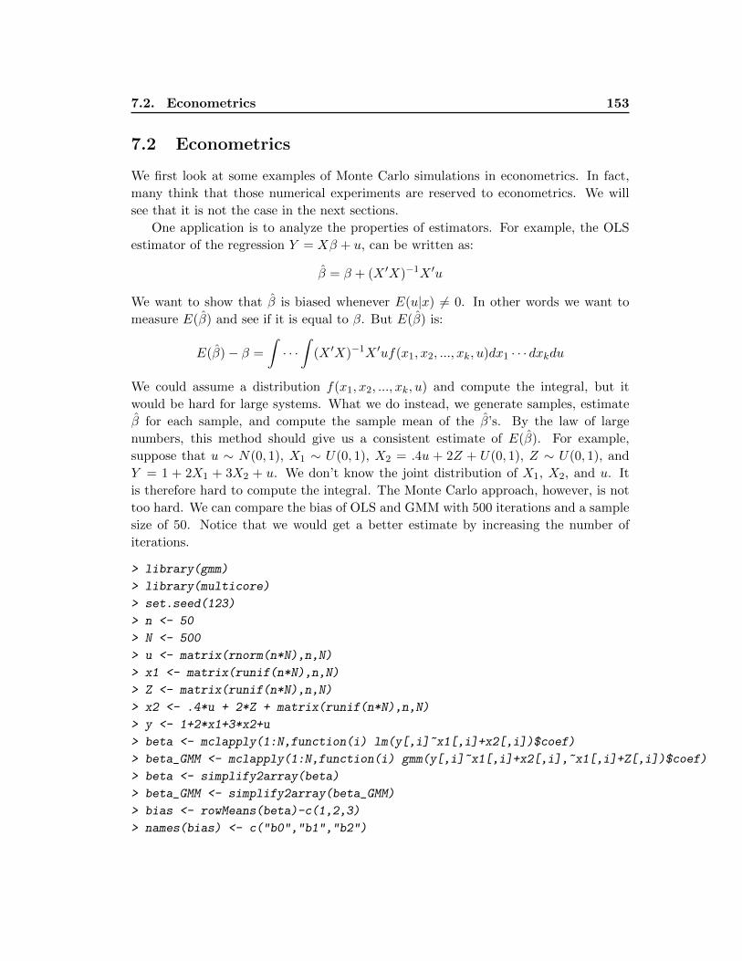
7.2. Econometrics 153
7.2 Econometrics
We first look at some examples of Monte Carlo simulations in econometrics. In fact,
many think that those numerical experiments are reserved to econometrics. We will
see that it is not the case in the next sections.
One application is to analyze the properties of estimators. For example, the OLS
estimator of the regression Y = Xβ + u, can be written as:
β = β + (X ′X)−1X ′u
We want to show that β is biased whenever E(u|x) 6= 0. In other words we want to
measure E(β) and see if it is equal to β. But E(β) is:
E(β)− β =
∫· · ·∫
(X ′X)−1X ′uf(x1, x2, ..., xk, u)dx1 · · · dxkdu
We could assume a distribution f(x1, x2, ..., xk, u) and compute the integral, but it
would be hard for large systems. What we do instead, we generate samples, estimate
β for each sample, and compute the sample mean of the β’s. By the law of large
numbers, this method should give us a consistent estimate of E(β). For example,
suppose that u ∼ N(0, 1), X1 ∼ U(0, 1), X2 = .4u + 2Z + U(0, 1), Z ∼ U(0, 1), and
Y = 1 + 2X1 + 3X2 + u. We don’t know the joint distribution of X1, X2, and u. It
is therefore hard to compute the integral. The Monte Carlo approach, however, is not
too hard. We can compare the bias of OLS and GMM with 500 iterations and a sample
size of 50. Notice that we would get a better estimate by increasing the number of
iterations.
> library(gmm)
> library(multicore)
> set.seed(123)
> n <- 50
> N <- 500
> u <- matrix(rnorm(n*N),n,N)
> x1 <- matrix(runif(n*N),n,N)
> Z <- matrix(runif(n*N),n,N)
> x2 <- .4*u + 2*Z + matrix(runif(n*N),n,N)
> y <- 1+2*x1+3*x2+u
> beta <- mclapply(1:N,function(i) lm(y[,i]~x1[,i]+x2[,i])$coef)
> beta_GMM <- mclapply(1:N,function(i) gmm(y[,i]~x1[,i]+x2[,i],~x1[,i]+Z[,i])$coef)
> beta <- simplify2array(beta)
> beta_GMM <- simplify2array(beta_GMM)
> bias <- rowMeans(beta)-c(1,2,3)
> names(bias) <- c("b0","b1","b2")
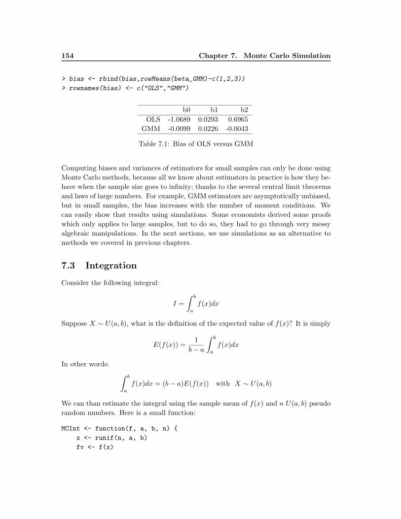
154 Chapter 7. Monte Carlo Simulation
> bias <- rbind(bias,rowMeans(beta_GMM)-c(1,2,3))
> rownames(bias) <- c("OLS","GMM")
b0 b1 b2
OLS -1.0689 0.0293 0.6965
GMM -0.0099 0.0226 -0.0043
Table 7.1: Bias of OLS versus GMM
Computing biases and variances of estimators for small samples can only be done using
Monte Carlo methods, because all we know about estimators in practice is how they be-
have when the sample size goes to infinity; thanks to the several central limit theorems
and laws of large numbers. For example, GMM estimators are asymptotically unbiased,
but in small samples, the bias increases with the number of moment conditions. We
can easily show that results using simulations. Some economists derived some proofs
which only applies to large samples, but to do so, they had to go through very messy
algebraic manipulations. In the next sections, we use simulations as an alternative to
methods we covered in previous chapters.
7.3 Integration
Consider the following integral:
I =
∫ b
af(x)dx
Suppose X ∼ U(a, b), what is the definition of the expected value of f(x)? It is simply
E(f(x)) =1
b− a
∫ b
af(x)dx
In other words: ∫ b
af(x)dx = (b− a)E(f(x)) with X ∼ U(a, b)
We can than estimate the integral using the sample mean of f(x) and n U(a, b) pseudo
random numbers. Here is a small function:
MCInt <- function(f, a, b, n) {
x <- runif(n, a, b)
fv <- f(x)
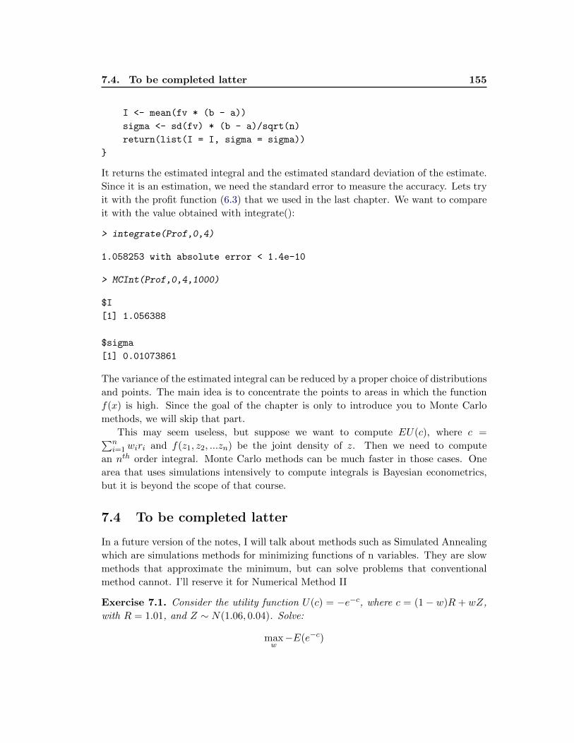
7.4. To be completed latter 155
I <- mean(fv * (b - a))
sigma <- sd(fv) * (b - a)/sqrt(n)
return(list(I = I, sigma = sigma))
}
It returns the estimated integral and the estimated standard deviation of the estimate.
Since it is an estimation, we need the standard error to measure the accuracy. Lets try
it with the profit function (6.3) that we used in the last chapter. We want to compare
it with the value obtained with integrate():
> integrate(Prof,0,4)
1.058253 with absolute error < 1.4e-10
> MCInt(Prof,0,4,1000)
$I
[1] 1.056388
$sigma
[1] 0.01073861
The variance of the estimated integral can be reduced by a proper choice of distributions
and points. The main idea is to concentrate the points to areas in which the function
f(x) is high. Since the goal of the chapter is only to introduce you to Monte Carlo
methods, we will skip that part.
This may seem useless, but suppose we want to compute EU(c), where c =∑ni=1wiri and f(z1, z2, ...zn) be the joint density of z. Then we need to compute
an nth order integral. Monte Carlo methods can be much faster in those cases. One
area that uses simulations intensively to compute integrals is Bayesian econometrics,
but it is beyond the scope of that course.
7.4 To be completed latter
In a future version of the notes, I will talk about methods such as Simulated Annealing
which are simulations methods for minimizing functions of n variables. They are slow
methods that approximate the minimum, but can solve problems that conventional
method cannot. I’ll reserve it for Numerical Method II
Exercise 7.1. Consider the utility function U(c) = −e−c, where c = (1− w)R + wZ,
with R = 1.01, and Z ∼ N(1.06, 0.04). Solve:
maxw−E(e−c)

156 Chapter 7. Monte Carlo Simulation
using a Monte Carlo simulation to compute the expected values. Compare the precision
of your solution for the number of points N = 50, 200, 1000, 5000.
Chapter 8
Differential Equations
Contents
8.1 Introduction . . . . . . . . . . . . . . . . . . . . . . . . . . . . . . 157
8.2 Finite Difference Methods for initial value problems . . . . . . 159
8.2.1 Euler’s Method . . . . . . . . . . . . . . . . . . . . . . . . . . . . . 160
8.2.2 Implicit Euler’s Method . . . . . . . . . . . . . . . . . . . . . . . . 161
8.2.3 Trapezoid Rule . . . . . . . . . . . . . . . . . . . . . . . . . . . . . 162
8.2.4 Runge-Kutta Method . . . . . . . . . . . . . . . . . . . . . . . . . 163
8.2.5 Example: Signaling Equilibrium . . . . . . . . . . . . . . . . . . . 165
8.3 Boundary values and the Shooting Method . . . . . . . . . . . . 167
8.3.1 Infinite Horizon Models . . . . . . . . . . . . . . . . . . . . . . . . 171
8.4 Projection Methods (incomplete) . . . . . . . . . . . . . . . . . . 178
8.5 Partial Differential Equation: The Heat Equation . . . . . . . . 184
8.5.1 Black and Scholes and the Heat Equation . . . . . . . . . . . . . . 189
8.6 R packages for differential equations . . . . . . . . . . . . . . . . 190
8.1 Introduction
In this chapter, we are interested in problems that can be written as:
dy
dx= f(x, y), (8.1)
where x ∈ [a, b], y ∈ Rn, and f : Rn+1 → Rn. This is called a system of first order
”Ordinary Differential Equation” (ODE). This is a very general representation of dif-
ferential equations because higher order equations can always be redefined as a first
order equation be an appropriate change of variable. For example, the second order
differential equation y′′(x) = f(y′(x), y, x) can be written as a system of two first order
differential equations: z′(x) = f(z, y, x), and y′(x) = z. The goal is to obtain the
solution y(x) that satisfies equation 8.1.
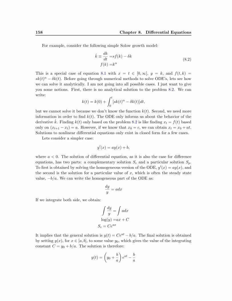
158 Chapter 8. Differential Equations
For example, consider the following simple Solow growth model:
k ≡ dk
dt=sf(k)− δk
f(k) =kα(8.2)
This is a special case of equation 8.1 with x = t ∈ [0,∞], y = k, and f(t, k) =
sk(t)α − δk(t). Before going through numerical methods to solve ODE’s, lets see how
we can solve it analytically. I am not going into all possible cases. I just want to give
you some notions. First, there is no analytical solution to the problem 8.2. We can
write:
k(t) = k(0) +
∫ t
0[sk(t)α − δk(t)]dt,
but we cannot solve it because we don’t know the function k(t). Second, we need more
information in order to find k(t). The ODE only informs us about the behavior of the
derivative k. Finding k(t) only based on the problem 8.2 is like finding xt = f(t) based
only on (xt+1 − xt) = a. However, if we know that x0 = c, we can obtain xt = x0 + at.
Solutions to nonlinear differential equations only exist in closed form for a few cases.
Lets consider a simpler case:
y′(x) = ay(x) + b,
where a < 0. The solution of differential equation, as it is also the case for difference
equations, has two parts: a complementary solution Sc and a particular solution Sp.
To first is obtained by solving the homogeneous version of the ODE, y′(x) = ay(x), and
the second is the solution for a particular value of x, which is often the steady state
value, −b/a. We can write the homogeneous part of the ODE as:
dy
y= adx
If we integrate both side, we obtain: ∫dy
y=
∫adx
log(y) =ax+ C
Sc = Ceax
It implies that the general solution is y(t) = Ceat − b/a. The final solution is obtained
by setting y(x), for x ∈ [a, b], to some value y0, which gives the value of the integrating
constant C = y0 + b/a. The solution is therefore:
y(t) =
(y0 +
b
a
)eat − b
a
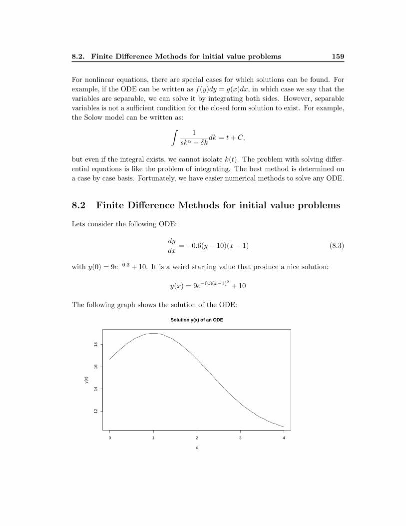
8.2. Finite Difference Methods for initial value problems 159
For nonlinear equations, there are special cases for which solutions can be found. For
example, if the ODE can be written as f(y)dy = g(x)dx, in which case we say that the
variables are separable, we can solve it by integrating both sides. However, separable
variables is not a sufficient condition for the closed form solution to exist. For example,
the Solow model can be written as:∫1
skα − δkdk = t+ C,
but even if the integral exists, we cannot isolate k(t). The problem with solving differ-
ential equations is like the problem of integrating. The best method is determined on
a case by case basis. Fortunately, we have easier numerical methods to solve any ODE.
8.2 Finite Difference Methods for initial value problems
Lets consider the following ODE:
dy
dx= −0.6(y − 10)(x− 1) (8.3)
with y(0) = 9e−0.3 + 10. It is a weird starting value that produce a nice solution:
y(x) = 9e−0.3(x−1)2
+ 10
The following graph shows the solution of the ODE:
0 1 2 3 4
1214
1618
Solution y(x) of an ODE
x
y(x)
160 Chapter 8. Differential Equations
8.2.1 Euler’s Method
Lets consider the general case:
y′(x) = f(x, y),
for x ∈ [a, b], and y(a) = y0. Lets consider n + 1 points xi, i = 0, ..., n, such that
xi = a+ ih, where h is the step size. The Euler’s method is based in the result:
y(xk+1)− y(xk) =
∫ xk+1
xk
f(x, y(x))dx
By the rectangle rule, the right hand side can be approximated by hf(xk, y(xk)), which
gives us the Euler’s algorithm:
yk+1 = yk + hf(xk, yk)
with the stating point (x, y) = (a, y0). The following figure show the result for the
problem 8.3 for different h.
f <- function(x, y) -0.6 * (y - 10) * (x - 1)
myODE <- function(f, n, a, b, y0) {
h <- (b - a)/n
x <- a + h * (0:n)
y <- y0
for (i in 2:(n + 1)) y[i] <- y[i - 1] + h * f(x[i - 1], y[i - 1])
return(list(x = x, y = y, h = h))
}
0 1 2 3 4
1012
1416
1820
The Euler's Method
x
y(x)
Trueh = 0.4h = 0.2h = 0.133
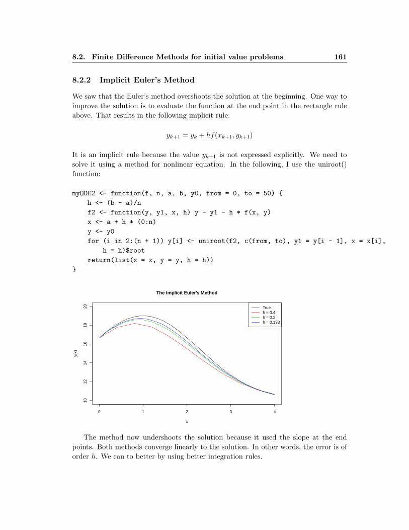
8.2. Finite Difference Methods for initial value problems 161
8.2.2 Implicit Euler’s Method
We saw that the Euler’s method overshoots the solution at the beginning. One way to
improve the solution is to evaluate the function at the end point in the rectangle rule
above. That results in the following implicit rule:
yk+1 = yk + hf(xk+1, yk+1)
It is an implicit rule because the value yk+1 is not expressed explicitly. We need to
solve it using a method for nonlinear equation. In the following, I use the uniroot()
function:
myODE2 <- function(f, n, a, b, y0, from = 0, to = 50) {
h <- (b - a)/n
f2 <- function(y, y1, x, h) y - y1 - h * f(x, y)
x <- a + h * (0:n)
y <- y0
for (i in 2:(n + 1)) y[i] <- uniroot(f2, c(from, to), y1 = y[i - 1], x = x[i],
h = h)$root
return(list(x = x, y = y, h = h))
}
0 1 2 3 4
1012
1416
1820
The Implicit Euler's Method
x
y(x)
Trueh = 0.4h = 0.2h = 0.133
The method now undershoots the solution because it used the slope at the end
points. Both methods converge linearly to the solution. In other words, the error is of
order h. We can to better by using better integration rules.
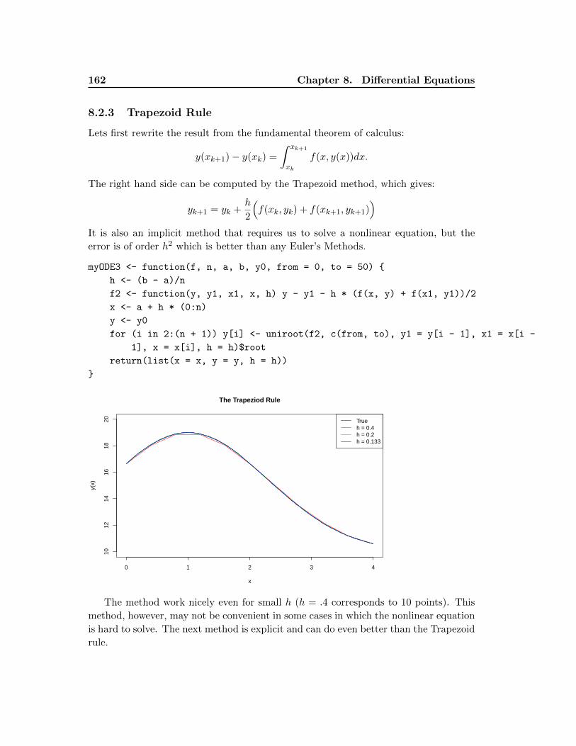
162 Chapter 8. Differential Equations
8.2.3 Trapezoid Rule
Lets first rewrite the result from the fundamental theorem of calculus:
y(xk+1)− y(xk) =
∫ xk+1
xk
f(x, y(x))dx.
The right hand side can be computed by the Trapezoid method, which gives:
yk+1 = yk +h
2
(f(xk, yk) + f(xk+1, yk+1)
)It is also an implicit method that requires us to solve a nonlinear equation, but the
error is of order h2 which is better than any Euler’s Methods.
myODE3 <- function(f, n, a, b, y0, from = 0, to = 50) {
h <- (b - a)/n
f2 <- function(y, y1, x1, x, h) y - y1 - h * (f(x, y) + f(x1, y1))/2
x <- a + h * (0:n)
y <- y0
for (i in 2:(n + 1)) y[i] <- uniroot(f2, c(from, to), y1 = y[i - 1], x1 = x[i -
1], x = x[i], h = h)$root
return(list(x = x, y = y, h = h))
}
0 1 2 3 4
1012
1416
1820
The Trapeziod Rule
x
y(x)
Trueh = 0.4h = 0.2h = 0.133
The method work nicely even for small h (h = .4 corresponds to 10 points). This
method, however, may not be convenient in some cases in which the nonlinear equation
is hard to solve. The next method is explicit and can do even better than the Trapezoid
rule.
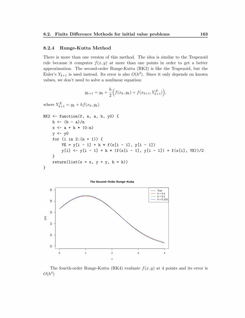
8.2. Finite Difference Methods for initial value problems 163
8.2.4 Runge-Kutta Method
There is more than one version of this method. The idea is similar to the Trapezoid
rule because it computes f(x, y) at more than one points in order to get a better
approximation. The second-order Runge-Kutta (RK2) is like the Trapezoid, but the
Euler’s Yk+1 is used instead. Its error is also O(h2). Since it only depends on known
values, we don’t need to solve a nonlinear equation:
yk+1 = yk +h
2
(f(xk, yk) + f(xk+1, Y
Ek+1)
),
where Y Ek+1 = yk + hf(xk, yk)
RK2 <- function(f, n, a, b, y0) {
h <- (b - a)/n
x <- a + h * (0:n)
y <- y0
for (i in 2:(n + 1)) {
YE = y[i - 1] + h * f(x[i - 1], y[i - 1])
y[i] <- y[i - 1] + h * (f(x[i - 1], y[i - 1]) + f(x[i], YE))/2
}
return(list(x = x, y = y, h = h))
}
0 1 2 3 4
1012
1416
1820
The Second−Order Runge−Kutta
x
y(x)
Trueh = 0.4h = 0.2h = 0.133
The fourth-order Runge-Kutta (RK4) evaluate f(x, y) at 4 points and its error is
O(h4)
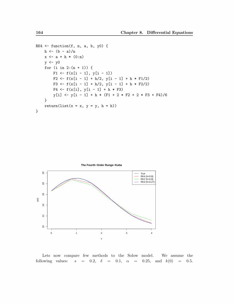
164 Chapter 8. Differential Equations
RK4 <- function(f, n, a, b, y0) {
h <- (b - a)/n
x <- a + h * (0:n)
y <- y0
for (i in 2:(n + 1)) {
F1 <- f(x[i - 1], y[i - 1])
F2 <- f(x[i - 1] + h/2, y[i - 1] + h * F1/2)
F3 <- f(x[i - 1] + h/2, y[i - 1] + h * F2/2)
F4 <- f(x[i], y[i - 1] + h * F3)
y[i] <- y[i - 1] + h * (F1 + 2 * F2 + 2 * F3 + F4)/6
}
return(list(x = x, y = y, h = h))
}
0 1 2 3 4
1012
1416
1820
The Fourth−Order Runge−Kutta
x
y(x)
TrueRK4 (h=0.8)RK2 (h=0.8)RK4 (h=0.27)
Lets now compare few methods to the Solow model. We assume the
following values: s = 0.2, δ = 0.1, α = 0.25, and k(0) = 0.5.
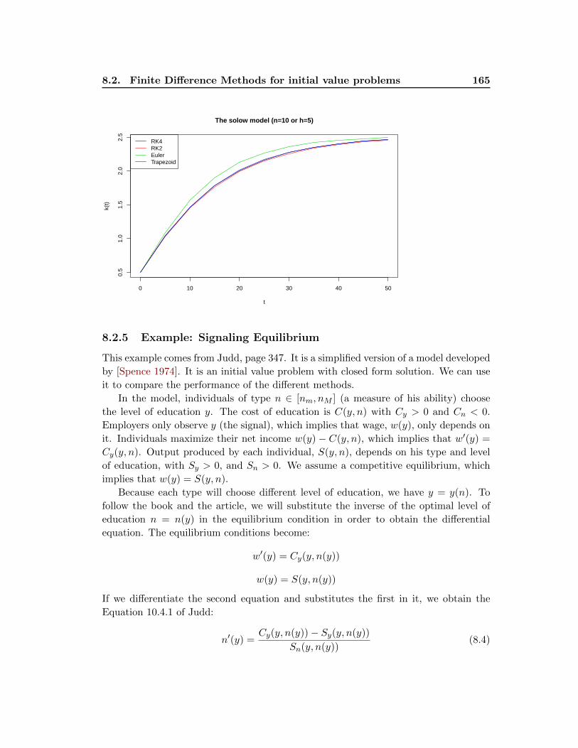
8.2. Finite Difference Methods for initial value problems 165
0 10 20 30 40 50
0.5
1.0
1.5
2.0
2.5
The solow model (n=10 or h=5)
t
k(t)
RK4RK2EulerTrapezoid
8.2.5 Example: Signaling Equilibrium
This example comes from Judd, page 347. It is a simplified version of a model developed
by [Spence 1974]. It is an initial value problem with closed form solution. We can use
it to compare the performance of the different methods.
In the model, individuals of type n ∈ [nm, nM ] (a measure of his ability) choose
the level of education y. The cost of education is C(y, n) with Cy > 0 and Cn < 0.
Employers only observe y (the signal), which implies that wage, w(y), only depends on
it. Individuals maximize their net income w(y) − C(y, n), which implies that w′(y) =
Cy(y, n). Output produced by each individual, S(y, n), depends on his type and level
of education, with Sy > 0, and Sn > 0. We assume a competitive equilibrium, which
implies that w(y) = S(y, n).
Because each type will choose different level of education, we have y = y(n). To
follow the book and the article, we will substitute the inverse of the optimal level of
education n = n(y) in the equilibrium condition in order to obtain the differential
equation. The equilibrium conditions become:
w′(y) = Cy(y, n(y))
w(y) = S(y, n(y))
If we differentiate the second equation and substitutes the first in it, we obtain the
Equation 10.4.1 of Judd:
n′(y) =Cy(y, n(y))− Sy(y, n(y))
Sn(y, n(y))(8.4)
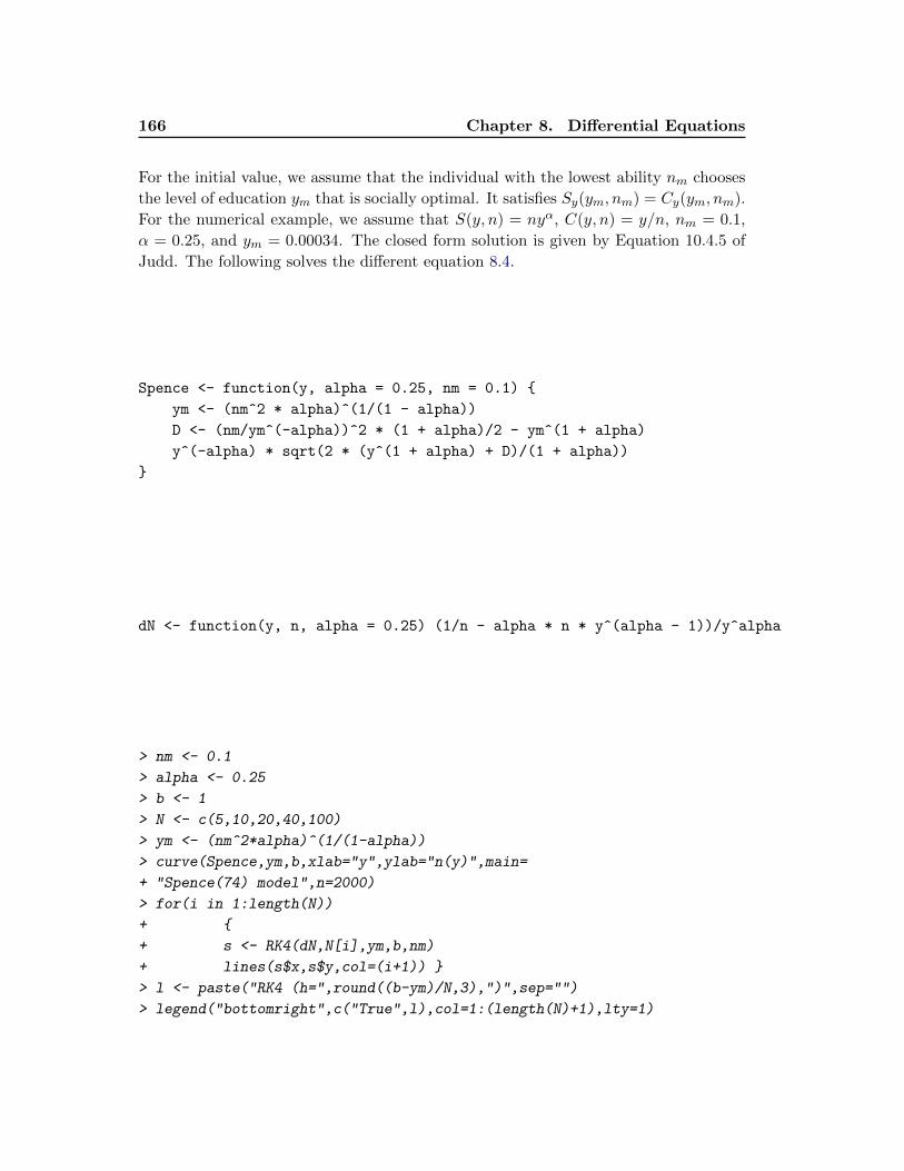
166 Chapter 8. Differential Equations
For the initial value, we assume that the individual with the lowest ability nm chooses
the level of education ym that is socially optimal. It satisfies Sy(ym, nm) = Cy(ym, nm).
For the numerical example, we assume that S(y, n) = nyα, C(y, n) = y/n, nm = 0.1,
α = 0.25, and ym = 0.00034. The closed form solution is given by Equation 10.4.5 of
Judd. The following solves the different equation 8.4.
Spence <- function(y, alpha = 0.25, nm = 0.1) {
ym <- (nm^2 * alpha)^(1/(1 - alpha))
D <- (nm/ym^(-alpha))^2 * (1 + alpha)/2 - ym^(1 + alpha)
y^(-alpha) * sqrt(2 * (y^(1 + alpha) + D)/(1 + alpha))
}
dN <- function(y, n, alpha = 0.25) (1/n - alpha * n * y^(alpha - 1))/y^alpha
> nm <- 0.1
> alpha <- 0.25
> b <- 1
> N <- c(5,10,20,40,100)
> ym <- (nm^2*alpha)^(1/(1-alpha))
> curve(Spence,ym,b,xlab="y",ylab="n(y)",main=
+ "Spence(74) model",n=2000)
> for(i in 1:length(N))
+ {
+ s <- RK4(dN,N[i],ym,b,nm)
+ lines(s$x,s$y,col=(i+1)) }
> l <- paste("RK4 (h=",round((b-ym)/N,3),")",sep="")
> legend("bottomright",c("True",l),col=1:(length(N)+1),lty=1)
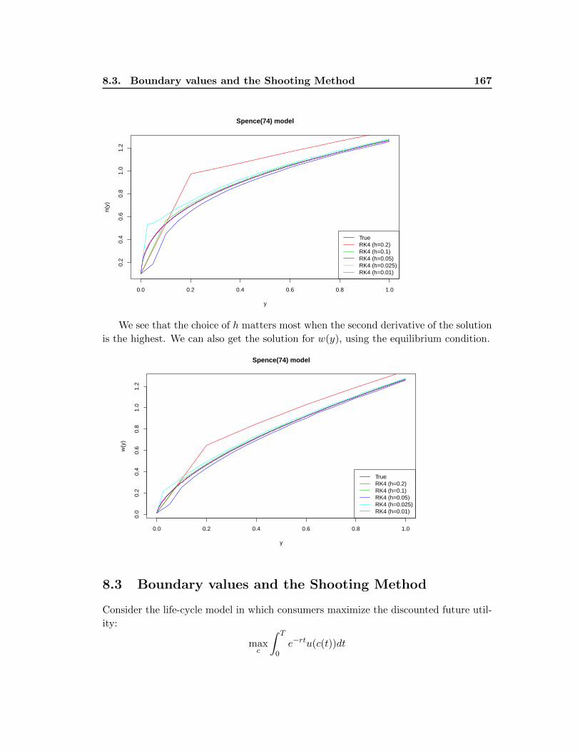
8.3. Boundary values and the Shooting Method 167
0.0 0.2 0.4 0.6 0.8 1.0
0.2
0.4
0.6
0.8
1.0
1.2
Spence(74) model
y
n(y)
TrueRK4 (h=0.2)RK4 (h=0.1)RK4 (h=0.05)RK4 (h=0.025)RK4 (h=0.01)
We see that the choice of h matters most when the second derivative of the solution
is the highest. We can also get the solution for w(y), using the equilibrium condition.
0.0 0.2 0.4 0.6 0.8 1.0
0.0
0.2
0.4
0.6
0.8
1.0
1.2
Spence(74) model
y
w(y
)
TrueRK4 (h=0.2)RK4 (h=0.1)RK4 (h=0.05)RK4 (h=0.025)RK4 (h=0.01)
8.3 Boundary values and the Shooting Method
Consider the life-cycle model in which consumers maximize the discounted future util-
ity:
maxc
∫ T
0e−rtu(c(t))dt
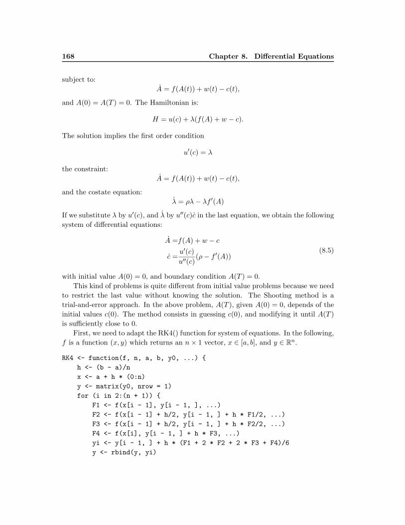
168 Chapter 8. Differential Equations
subject to:
A = f(A(t)) + w(t)− c(t),
and A(0) = A(T ) = 0. The Hamiltonian is:
H = u(c) + λ(f(A) + w − c).
The solution implies the first order condition
u′(c) = λ
the constraint:
A = f(A(t)) + w(t)− c(t),
and the costate equation:
λ = ρλ− λf ′(A)
If we substitute λ by u′(c), and λ by u′′(c)c in the last equation, we obtain the following
system of differential equations:
A =f(A) + w − c
c =u′(c)
u′′(c)(ρ− f ′(A))
(8.5)
with initial value A(0) = 0, and boundary condition A(T ) = 0.
This kind of problems is quite different from initial value problems because we need
to restrict the last value without knowing the solution. The Shooting method is a
trial-and-error approach. In the above problem, A(T ), given A(0) = 0, depends of the
initial values c(0). The method consists in guessing c(0), and modifying it until A(T )
is sufficiently close to 0.
First, we need to adapt the RK4() function for system of equations. In the following,
f is a function (x, y) which returns an n× 1 vector, x ∈ [a, b], and y ∈ Rn.
RK4 <- function(f, n, a, b, y0, ...) {
h <- (b - a)/n
x <- a + h * (0:n)
y <- matrix(y0, nrow = 1)
for (i in 2:(n + 1)) {
F1 <- f(x[i - 1], y[i - 1, ], ...)
F2 <- f(x[i - 1] + h/2, y[i - 1, ] + h * F1/2, ...)
F3 <- f(x[i - 1] + h/2, y[i - 1, ] + h * F2/2, ...)
F4 <- f(x[i], y[i - 1, ] + h * F3, ...)
yi <- y[i - 1, ] + h * (F1 + 2 * F2 + 2 * F3 + F4)/6
y <- rbind(y, yi)
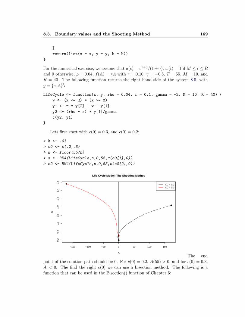
8.3. Boundary values and the Shooting Method 169
}
return(list(x = x, y = y, h = h))
}
For the numerical exercise, we assume that u(c) = c1+γ/(1+γ), w(t) = 1 if M ≤ t ≤ Rand 0 otherwise, ρ = 0.04, f(A) = rA with r = 0.10, γ = −0.5, T = 55, M = 10, and
R = 40. The following function returns the right hand side of the system 8.5, with
y = {c, A}′:
LifeCycle <- function(x, y, rho = 0.04, r = 0.1, gamma = -2, M = 10, R = 40) {
w <- (x <= R) * (x >= M)
y1 <- r * y[2] + w - y[1]
y2 <- (rho - r) * y[1]/gamma
c(y2, y1)
}
Lets first start with c(0) = 0.3, and c(0) = 0.2:
> h <- .01
> c0 <- c(.2,.3)
> n <- floor(55/h)
> s <- RK4(LifeCycle,n,0,55,c(c0[1],0))
> s2 <- RK4(LifeCycle,n,0,55,c(c0[2],0))
−150 −100 −50 0 50 100 150
0.2
0.4
0.6
0.8
1.0
1.2
1.4
1.6
Life Cycle Model: The Shooting Method
A
C
●
●
●
● C0 = 0.2C0 = 0.3
The end
point of the solution path should be 0. For c(0) = 0.2, A(55) > 0, and for c(0) = 0.3,
A < 0. The find the right c(0) we can use a bisection method. The following is a
function that can be used in the Bisection() function of Chapter 5:
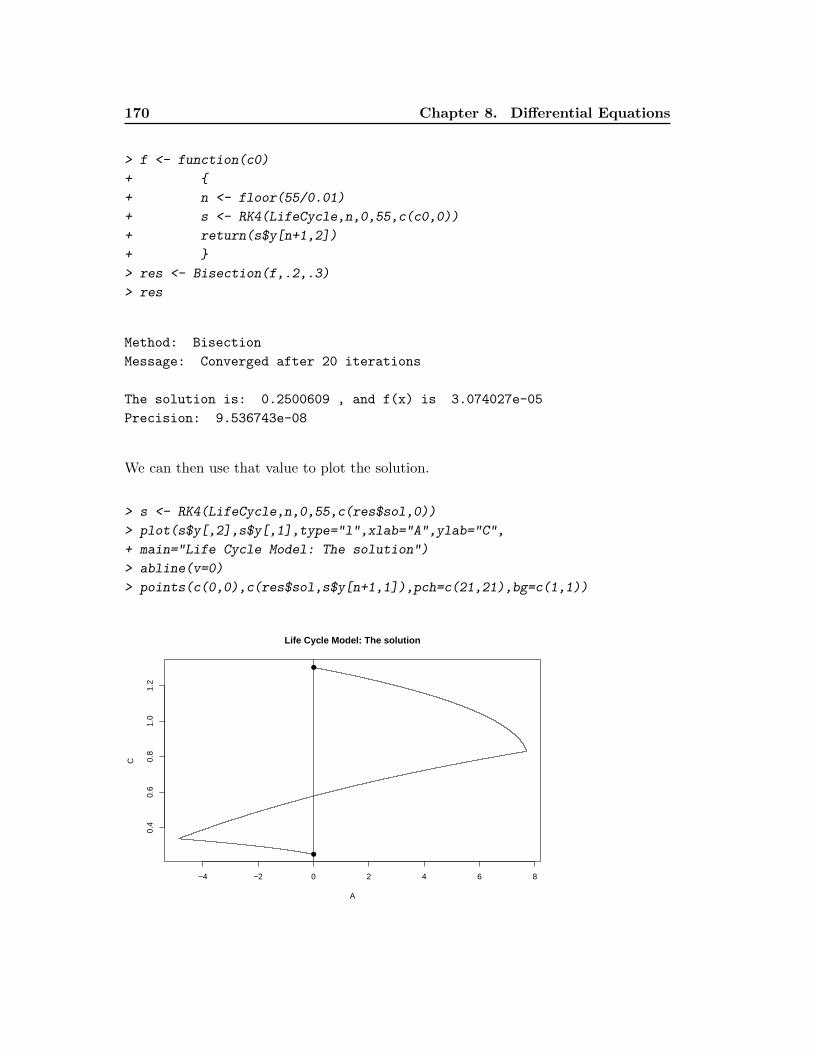
170 Chapter 8. Differential Equations
> f <- function(c0)
+ {
+ n <- floor(55/0.01)
+ s <- RK4(LifeCycle,n,0,55,c(c0,0))
+ return(s$y[n+1,2])
+ }
> res <- Bisection(f,.2,.3)
> res
Method: Bisection
Message: Converged after 20 iterations
The solution is: 0.2500609 , and f(x) is 3.074027e-05
Precision: 9.536743e-08
We can then use that value to plot the solution.
> s <- RK4(LifeCycle,n,0,55,c(res$sol,0))
> plot(s$y[,2],s$y[,1],type="l",xlab="A",ylab="C",
+ main="Life Cycle Model: The solution")
> abline(v=0)
> points(c(0,0),c(res$sol,s$y[n+1,1]),pch=c(21,21),bg=c(1,1))
−4 −2 0 2 4 6 8
0.4
0.6
0.8
1.0
1.2
Life Cycle Model: The solution
A
C
●
●
8.3. Boundary values and the Shooting Method 171
8.3.1 Infinite Horizon Models
Consider the following model:
maxc
∫ ∞0
e−ρtu(c)dt
subject to k = f(k) − c, and k(0) = k0. We don’t have explicit boundary conditions,
but we have to assume that limt→∞ |k(t)| <∞ (which also implies the convergence of
|c(t)|). We know for the above model that the only possible path is the one that will
make k(t) and c(t) converge to their respective steady state values, k∗ and c∗. The first
method is to forward shooting and it consists in choosing the path that leads as close
as possible to the steady state. The following algorithm is the one proposed on page
357 of Judd, and it is for the case in which k0 < k∗. We also use the specification given
on page 359.
growth <- function(x, y) {
y1 <- -(0.05 - 0.05 * y[2]^(-0.75)) * y[1]/2
y2 <- 0.2 * y[2]^0.25 - y[1]
c(y1, y2)
}
RK4G <- function(f, h, y0, maxit = 1000) {
#The difference: it stops when either df/dy<0
x <- 0
y <- matrix(y0, nrow = 1)
i <- 1
while (TRUE) {
F1 <- f(x[i], y[i, ])
F2 <- f(x[i] + h/2, y[i, ] + h * F1/2)
F3 <- f(x[i] + h/2, y[i, ] + h * F2/2)
F4 <- f(x[i] + h, y[i, ] + h * F3)
y1 <- y[i, ] + h * (F1 + 2 * F2 + 2 * F3 + F4)/6
x <- c(x, x[i] + h)
y <- rbind(y, y1)
if (any(f(x[i + 1], y1) < 0))
break
if (i > maxit) {
warning("maxit reached")
break
}
i <- i + 1
172 Chapter 8. Differential Equations
}
return(list(T = i, y = y, x = x))
}
fShooting <- function(f, k0, h = 0.01, eps = 1e-07, maxit = 20) {
cL <- 0
cH <- 0.2 * k0^0.25
cSteady <- 0.2
i <- 1
while (TRUE) {
c0 <- (cL + cH)/2
res <- RK4G(f, h, c(c0, k0), maxit = 2000)
T <- res$T + 1
if (abs(res$y[T, 1] - cSteady) < eps)
break
if (i > maxit) {
warning("Maxit reached")
break
}
ydot <- f(res$x[T], res$y[T, ])
if (ydot[1] < 0)
cL <- c0 else cH <- c0
i <- i + 1
}
return(res)
}
> res <- fShooting(growth,.2,eps=1e-3,maxit=1000,h=.1)
> k <- res$y[,2]
> c <- res$y[,1]
> curve(.2*x^.25,0,1.50,xlab="K(t)",ylab="C(t)",n=1000,xlim=c(-.2,1.8),
+ main="Infinite-Horizon problem with Forward Shooting",lwd=2)
> abline(v=1,lwd=2,col=2)
> text(1.075,.02,expression(dot(C)==0),col=2)
> text(1.6,.22,expression(dot(K)==0),col=1)
> lines(k,c,col=4,lwd=4)
> text(k[20],c[20],"Stable Path",col=4,pos=4)
> points(k[1],c[1],pch=21,bg=4)
> text(k[1]+.05,c[1],paste("(",round(k[1],3),", ",round(c[1],4),")",sep=""),pos=1,col=4)
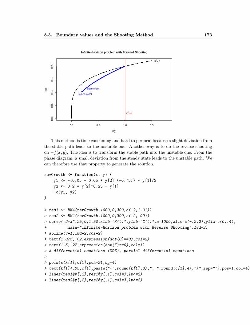
8.3. Boundary values and the Shooting Method 173
0.0 0.5 1.0 1.5
0.00
0.05
0.10
0.15
0.20
Infinite−Horizon problem with Forward Shooting
K(t)
C(t
)
C⋅ = 0
K⋅ = 0
Stable Path●
(0.2, 0.1027)
This method is time consuming and hard to perform because a slight deviation from
the stable path leads to the unstable one. Another way is to do the reverse shooting
on −f(x, y). The idea is to transform the stable path into the unstable one. From the
phase diagram, a small deviation from the steady state leads to the unstable path. We
can therefore use that property to generate the solution.
revGrowth <- function(x, y) {
y1 <- -(0.05 - 0.05 * y[2]^(-0.75)) * y[1]/2
y2 <- 0.2 * y[2]^0.25 - y[1]
-c(y1, y2)
}
> res1 <- RK4(revGrowth,1000,0,300,c(.2,1.01))
> res2 <- RK4(revGrowth,1000,0,300,c(.2,.99))
> curve(.2*x^.25,0,1.50,xlab="K(t)",ylab="C(t)",n=1000,xlim=c(-.2,2),ylim=c(0,.4),
+ main="Infinite-Horizon problem with Reverse Shooting",lwd=2)
> abline(v=1,lwd=2,col=2)
> text(1.075,.02,expression(dot(C)==0),col=2)
> text(1.6,.22,expression(dot(K)==0),col=1)
> # differential equations (ODE), partial differential equations
>
> points(k[1],c[1],pch=21,bg=4)
> text(k[1]+.05,c[1],paste("(",round(k[1],3),", ",round(c[1],4),")",sep=""),pos=1,col=4)
> lines(res1$y[,2],res1$y[,1],col=3,lwd=2)
> lines(res2$y[,2],res2$y[,1],col=3,lwd=2)
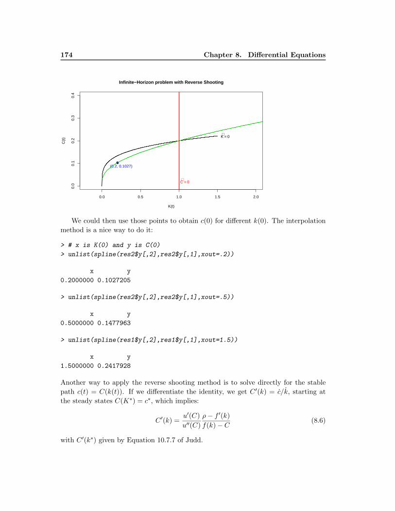
174 Chapter 8. Differential Equations
0.0 0.5 1.0 1.5 2.0
0.0
0.1
0.2
0.3
0.4
Infinite−Horizon problem with Reverse Shooting
K(t)
C(t
)
C⋅ = 0
K⋅ = 0
●
(0.2, 0.1027)
We could then use those points to obtain c(0) for different k(0). The interpolation
method is a nice way to do it:
> # x is K(0) and y is C(0)
> unlist(spline(res2$y[,2],res2$y[,1],xout=.2))
x y
0.2000000 0.1027205
> unlist(spline(res2$y[,2],res2$y[,1],xout=.5))
x y
0.5000000 0.1477963
> unlist(spline(res1$y[,2],res1$y[,1],xout=1.5))
x y
1.5000000 0.2417928
Another way to apply the reverse shooting method is to solve directly for the stable
path c(t) = C(k(t)). If we differentiate the identity, we get C ′(k) = c/k, starting at
the steady states C(K∗) = c∗, which implies:
C ′(k) =u′(C)
u′′(C)
ρ− f ′(k)
f(k)− C(8.6)
with C ′(k∗) given by Equation 10.7.7 of Judd.
8.3. Boundary values and the Shooting Method 175
Exercise 8.1. Replicate Table 10.2 of Judd, using the reverse shooting method applied
to the differential equation 8.6
Exercise 8.2. Answer Exercises 2, 5, and 6 of Judd (Chapter 10)
We conclude the section with an example of reverse shooting for multidimensional
problems. We consider the growth model with 3 sectors presented in exercise 7, with
u(c) = log(c), ρ = 0.05, α1 = 0.25, α2 = 0.35, α3 = 0.4, γ1 = 10, γ2 = 50, γ3 = 100,
and ki(0) = 0.5 for i = 1, 2, 3. First, we need to compute the steady state. I don’t want
to compute it manually, so I will use a method from Chapter 5. First, the solution
implies the following differential equations.
λi = ρλi −ρkαi−1i
C,
ki = Ii,
for i = 1, 2, 3 with
λi =1 + 2γiIi
C
and
C = ρ
(kα11
α1+kα22
α2+kα33
α3
)−(I1 + I2 + I3 + γ1I
21 + γ2I
22 + γ3I
23
)The steady state values are k∗i = 1, I∗i = 0, and λ∗i = 1/C. There is two approaches
to solve the problem. First, we can follow the procedure on page 361 of Judd, and
solve for Ii(t) using the maximum principle (the first order conditions), and substitute
the solution into the differential equations. However, there is no closed form solution
Ii(t). We can solve it using a nonlinear solver but it may be unstable because there are
multiple solutions. The following follows that method:
MGrowth <- function(x, y) {
alpha <- c(0.25, 0.35, 0.4)
rho = 0.05
gamma = c(10, 50, 100)
I0 <- c(0, 0, 0)
I <- function(I, K, Lambda) {
C <- sum(rho * K^alpha/alpha) - sum(I) - sum(gamma * I^2)
C * Lambda - 1 - 2 * gamma * I
}
Iv <- Broyden(I, I0, K = y[1:3], Lambda = y[4:6])$sol
C <- sum(rho * y[1:3]^alpha/alpha) - sum(Iv) - sum(gamma * Iv^2)
dy2 <- rho * y[4:6] - rho * y[1:3]^(alpha - 1)/C
return(-c(Iv, dy2))
}
176 Chapter 8. Differential Equations
> SteadyC <- sum(rho/alpha)
> SteadyK <- c(1,1,1)
> SteadyL <- rep(1/SteadyC,3)
> y <- c(SteadyK*1.001,SteadyL)
> res1 <- RK4(MGrowth, n, 0, T, y)
I am not showing the result because it is not satisfying. In the second method, I
substitute the λi and λi by Ii and Ii. We replace λi by
λi =1 + 2γiIi
C
and λi by
λi = −1 + 2γiIiC2
C +2γiIiC
Because dotC depends on all ki and Ii, we need to solve a linear system of equations
to obtain the 6 differential equations.
MGrowth2 <- function(x, y) {
alpha <- c(0.25, 0.35, 0.4)
rho = 0.05
gamma = c(10, 50, 100)
K <- y[1:3]
I <- y[4:6]
C <- sum(rho * y[1:3]^alpha/alpha) - sum(I) - sum(gamma * I^2)
Ai <- -1/C^2 * (1 + 2 * gamma * I)
Bi <- 2 * gamma/C
Ei <- rho * (1 + 2 * gamma * I)/C - rho * K^(alpha - 1)/C
A <- c(rho * K^(alpha - 1), -(1 + 2 * gamma * I))
W <- Ai %o% A
diag(W[1:3, 4:6]) <- diag(W[1:3, 4:6]) + Bi
W <- rbind(W, cbind(diag(3), 0, 0, 0))
-solve(W, c(Ei, I))
}
> T <- 73
> n <- 400
> SteadyK <- c(1,1,1)
> y <- c(SteadyK*1.01,rep(-0.01,3))
> res <- RK4(MGrowth2, n, 0, T, y)
> y <- c(SteadyK*.99,rep(0.01,3))
> res1 <- RK4(MGrowth2, n, 0, T, y)
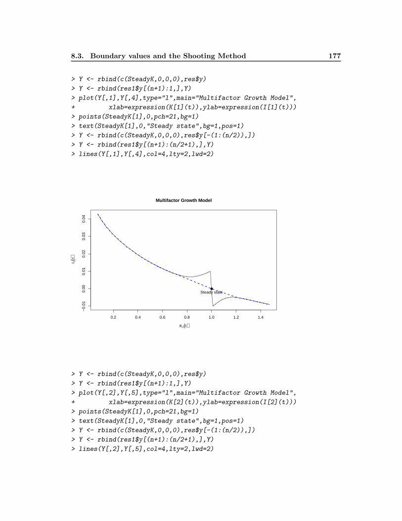
8.3. Boundary values and the Shooting Method 177
> Y <- rbind(c(SteadyK,0,0,0),res$y)
> Y <- rbind(res1$y[(n+1):1,],Y)
> plot(Y[,1],Y[,4],type="l",main="Multifactor Growth Model",
+ xlab=expression(K[1](t)),ylab=expression(I[1](t)))
> points(SteadyK[1],0,pch=21,bg=1)
> text(SteadyK[1],0,"Steady state",bg=1,pos=1)
> Y <- rbind(c(SteadyK,0,0,0),res$y[-(1:(n/2)),])
> Y <- rbind(res1$y[(n+1):(n/2+1),],Y)
> lines(Y[,1],Y[,4],col=4,lty=2,lwd=2)
0.2 0.4 0.6 0.8 1.0 1.2 1.4
−0.
010.
000.
010.
020.
030.
04
Multifactor Growth Model
K1(t)
I 1(t)
●
Steady state
> Y <- rbind(c(SteadyK,0,0,0),res$y)
> Y <- rbind(res1$y[(n+1):1,],Y)
> plot(Y[,2],Y[,5],type="l",main="Multifactor Growth Model",
+ xlab=expression(K[2](t)),ylab=expression(I[2](t)))
> points(SteadyK[1],0,pch=21,bg=1)
> text(SteadyK[1],0,"Steady state",bg=1,pos=1)
> Y <- rbind(c(SteadyK,0,0,0),res$y[-(1:(n/2)),])
> Y <- rbind(res1$y[(n+1):(n/2+1),],Y)
> lines(Y[,2],Y[,5],col=4,lty=2,lwd=2)
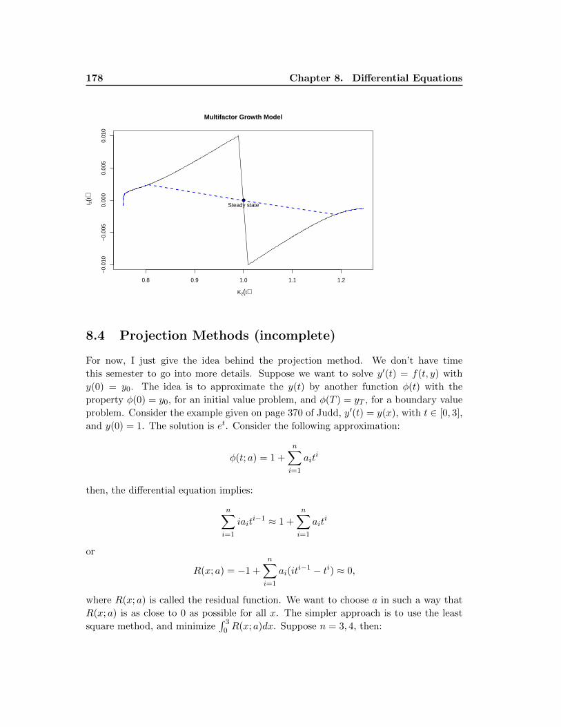
178 Chapter 8. Differential Equations
0.8 0.9 1.0 1.1 1.2
−0.
010
−0.
005
0.00
00.
005
0.01
0
Multifactor Growth Model
K2(t)
I 2(t) ●
Steady state
8.4 Projection Methods (incomplete)
For now, I just give the idea behind the projection method. We don’t have time
this semester to go into more details. Suppose we want to solve y′(t) = f(t, y) with
y(0) = y0. The idea is to approximate the y(t) by another function φ(t) with the
property φ(0) = y0, for an initial value problem, and φ(T ) = yT , for a boundary value
problem. Consider the example given on page 370 of Judd, y′(t) = y(x), with t ∈ [0, 3],
and y(0) = 1. The solution is et. Consider the following approximation:
φ(t; a) = 1 +n∑i=1
aiti
then, the differential equation implies:
n∑i=1
iaiti−1 ≈ 1 +
n∑i=1
aiti
or
R(x; a) = −1 +
n∑i=1
ai(iti−1 − ti) ≈ 0,
where R(x; a) is called the residual function. We want to choose a in such a way that
R(x; a) is as close to 0 as possible for all x. The simpler approach is to use the least
square method, and minimize∫ 30 R(x; a)dx. Suppose n = 3, 4, then:
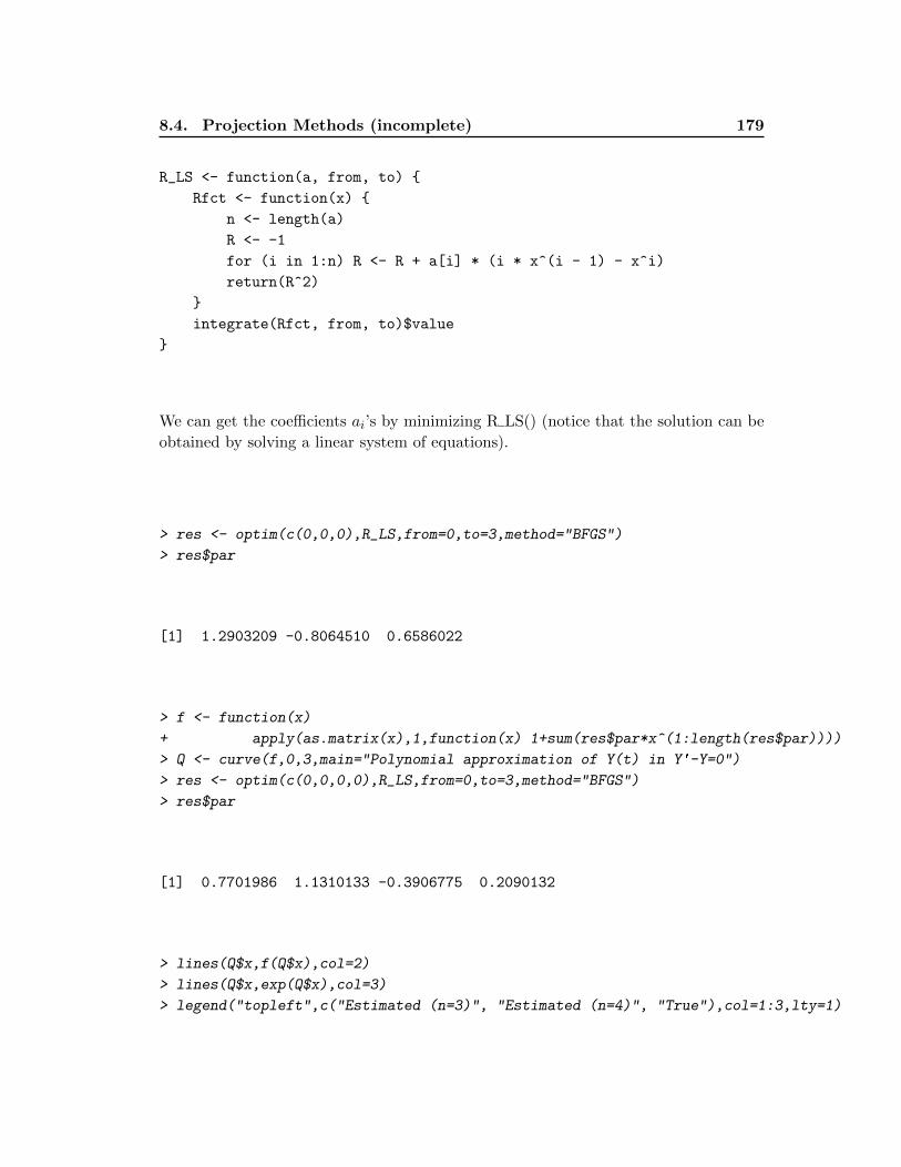
8.4. Projection Methods (incomplete) 179
R_LS <- function(a, from, to) {
Rfct <- function(x) {
n <- length(a)
R <- -1
for (i in 1:n) R <- R + a[i] * (i * x^(i - 1) - x^i)
return(R^2)
}
integrate(Rfct, from, to)$value
}
We can get the coefficients ai’s by minimizing R LS() (notice that the solution can be
obtained by solving a linear system of equations).
> res <- optim(c(0,0,0),R_LS,from=0,to=3,method="BFGS")
> res$par
[1] 1.2903209 -0.8064510 0.6586022
> f <- function(x)
+ apply(as.matrix(x),1,function(x) 1+sum(res$par*x^(1:length(res$par))))
> Q <- curve(f,0,3,main="Polynomial approximation of Y(t) in Y'-Y=0")
> res <- optim(c(0,0,0,0),R_LS,from=0,to=3,method="BFGS")
> res$par
[1] 0.7701986 1.1310133 -0.3906775 0.2090132
> lines(Q$x,f(Q$x),col=2)
> lines(Q$x,exp(Q$x),col=3)
> legend("topleft",c("Estimated (n=3)", "Estimated (n=4)", "True"),col=1:3,lty=1)
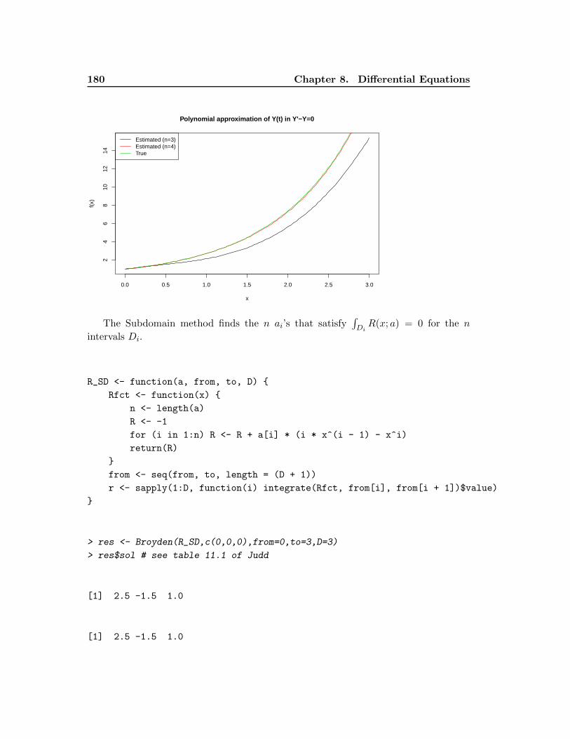
180 Chapter 8. Differential Equations
0.0 0.5 1.0 1.5 2.0 2.5 3.0
24
68
1012
14
Polynomial approximation of Y(t) in Y'−Y=0
x
f(x)
Estimated (n=3)Estimated (n=4)True
The Subdomain method finds the n ai’s that satisfy∫DiR(x; a) = 0 for the n
intervals Di.
R_SD <- function(a, from, to, D) {
Rfct <- function(x) {
n <- length(a)
R <- -1
for (i in 1:n) R <- R + a[i] * (i * x^(i - 1) - x^i)
return(R)
}
from <- seq(from, to, length = (D + 1))
r <- sapply(1:D, function(i) integrate(Rfct, from[i], from[i + 1])$value)
}
> res <- Broyden(R_SD,c(0,0,0),from=0,to=3,D=3)
> res$sol # see table 11.1 of Judd
[1] 2.5 -1.5 1.0
[1] 2.5 -1.5 1.0
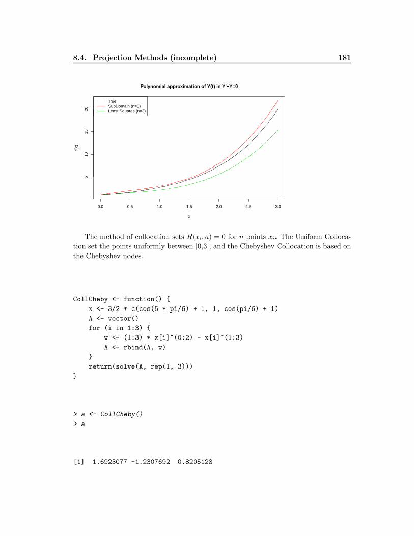
8.4. Projection Methods (incomplete) 181
0.0 0.5 1.0 1.5 2.0 2.5 3.0
510
1520
Polynomial approximation of Y(t) in Y'−Y=0
x
f(x)
TrueSubDomain (n=3)Least Squares (n=3)
The method of collocation sets R(xi, a) = 0 for n points xi. The Uniform Colloca-
tion set the points uniformly between [0,3], and the Chebyshev Collocation is based on
the Chebyshev nodes.
CollCheby <- function() {
x <- 3/2 * c(cos(5 * pi/6) + 1, 1, cos(pi/6) + 1)
A <- vector()
for (i in 1:3) {
w <- (1:3) * x[i]^(0:2) - x[i]^(1:3)
A <- rbind(A, w)
}
return(solve(A, rep(1, 3)))
}
> a <- CollCheby()
> a
[1] 1.6923077 -1.2307692 0.8205128
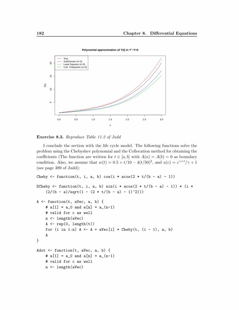
182 Chapter 8. Differential Equations
0.0 0.5 1.0 1.5 2.0 2.5 3.0
510
1520
Polynomial approximation of Y(t) in Y'−Y=0
x
f(x)
TrueSubDomain (n=3)Least Squares (n=3)Coll. Chebyshev (n=3)
Exercise 8.3. Reproduce Table 11.2 of Judd
I conclude the section with the life cycle model. The following functions solve the
problem using the Chebyshev polynomial and the Collocation method for obtaining the
coefficients (The function are written for t ∈ [a, b] with A(a) = A(b) = 0 as boundary
condition. Also, we assume that w(t) = 0.5 + t/10 − 4(t/50)2, and u(c) = cγ+1/γ + 1
(see page 389 of Judd):
Cheby <- function(t, i, a, b) cos(i * acos(2 * t/(b - a) - 1))
DCheby <- function(t, i, a, b) sin(i * acos(2 * t/(b - a) - 1)) * (i *
(2/(b - a)/sqrt(1 - (2 * t/(b - a) - 1)^2)))
A <- function(t, aVec, a, b) {
# a[1] = a_0 and a[n] = a_(n-1)
# valid for c as well
n <- length(aVec)
A <- rep(0, length(t))
for (i in 1:n) A <- A + aVec[i] * Cheby(t, (i - 1), a, b)
A
}
Adot <- function(t, aVec, a, b) {
# a[1] = a_0 and a[n] = a_(n-1)
# valid for c as well
n <- length(aVec)
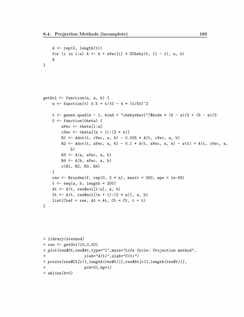
8.4. Projection Methods (incomplete) 183
A <- rep(0, length(t))
for (i in 1:n) A <- A + aVec[i] * DCheby(t, (i - 1), a, b)
A
}
getSol <- function(n, a, b) {
w <- function(t) 0.5 + t/10 - 4 * (t/50)^2
t <- gauss.quad(n - 1, kind = "chebyshev1")$node * (b - a)/2 + (b - a)/2
f <- function(theta) {
aVec <- theta[1:n]
cVec <- theta[(n + 1):(2 * n)]
R1 <- Adot(t, cVec, a, b) - 0.025 * A(t, cVec, a, b)
R2 <- Adot(t, aVec, a, b) - 0.1 * A(t, aVec, a, b) - w(t) + A(t, cVec, a,
b)
R3 <- A(a, aVec, a, b)
R4 <- A(b, aVec, a, b)
c(R1, R2, R3, R4)
}
res <- Broyden(f, rep(0, 2 * n), maxit = 300, eps = 1e-09)
t <- seq(a, b, length = 200)
At <- A(t, res$sol[1:n], a, b)
Ct <- A(t, res$sol[(n + 1):(2 * n)], a, b)
list(Coef = res, At = At, Ct = Ct, t = t)
}
> library(statmod)
> res <- getSol(10,0,50)
> plot(res$Ct,res$At,type="l",main="Life Cycle: Projection method",
+ ylab="A(t)",xlab="C(t)")
> points(res$Ct[c(1,length(res$t))],res$At[c(1,length(res$t))],
+ pch=21,bg=1)
> abline(h=0)
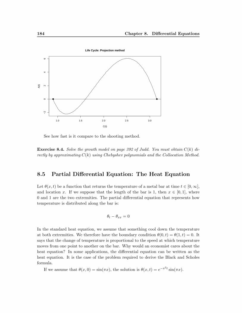
184 Chapter 8. Differential Equations
1.0 1.5 2.0 2.5 3.0
−2
02
46
Life Cycle: Projection method
C(t)
A(t
)
● ●
See how fast is it compare to the shooting method.
Exercise 8.4. Solve the growth model on page 392 of Judd. You must obtain C(k) di-
rectly by approximating C(k) using Chebyshev polynomials and the Collocation Method.
8.5 Partial Differential Equation: The Heat Equation
Let θ(x, t) be a function that returns the temperature of a metal bar at time t ∈ [0,∞],
and location x. If we suppose that the length of the bar is 1, then x ∈ [0, 1], where
0 and 1 are the two extremities. The partial differential equation that represents how
temperature is distributed along the bar is:
θt − θxx = 0
In the standard heat equation, we assume that something cool down the temperature
at both extremities. We therefore have the boundary condition θ(0, t) = θ(1, t) = 0. It
says that the change of temperature is proportional to the speed at which temperature
moves from one point to another on the bar. Why would an economist cares about the
heat equation? In some applications, the differential equation can be written as the
heat equation. It is the case of the problem required to derive the Black and Scholes
formula.
If we assume that θ(x, 0) = sin(πx), the solution is θ(x, t) = e−π2t sin(πx).
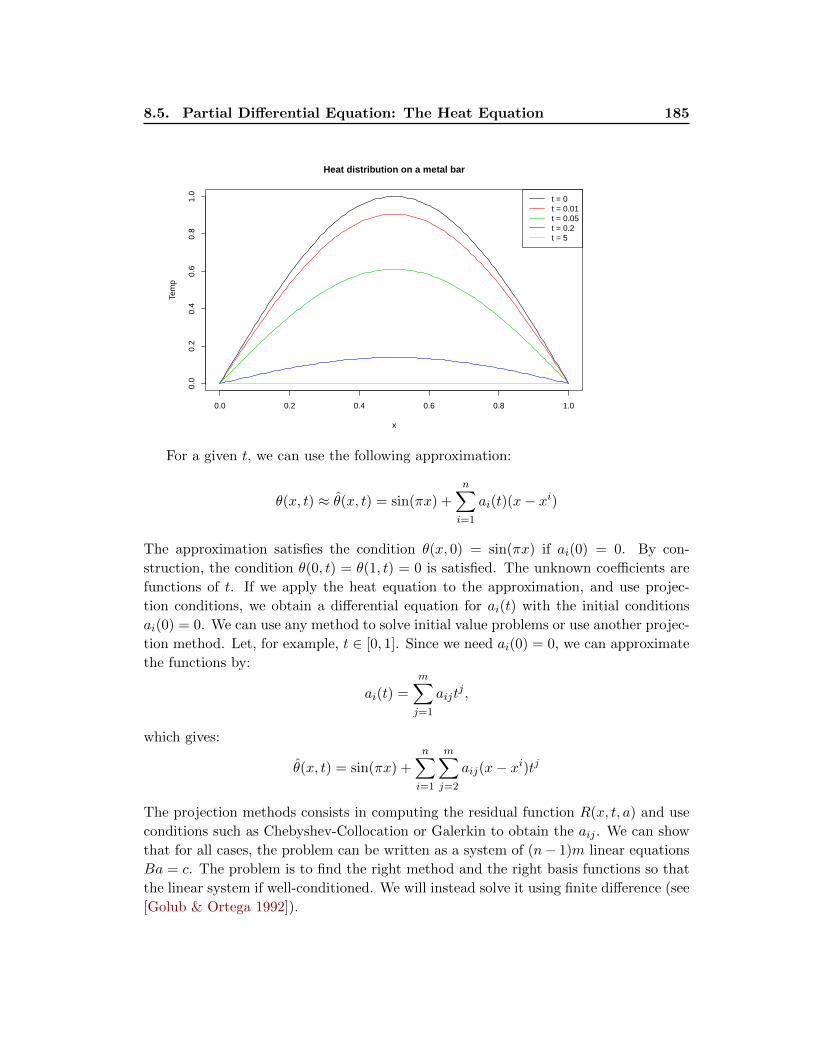
8.5. Partial Differential Equation: The Heat Equation 185
0.0 0.2 0.4 0.6 0.8 1.0
0.0
0.2
0.4
0.6
0.8
1.0
Heat distribution on a metal bar
x
Tem
p
t = 0t = 0.01t = 0.05t = 0.2t = 5
For a given t, we can use the following approximation:
θ(x, t) ≈ θ(x, t) = sin(πx) +n∑i=1
ai(t)(x− xi)
The approximation satisfies the condition θ(x, 0) = sin(πx) if ai(0) = 0. By con-
struction, the condition θ(0, t) = θ(1, t) = 0 is satisfied. The unknown coefficients are
functions of t. If we apply the heat equation to the approximation, and use projec-
tion conditions, we obtain a differential equation for ai(t) with the initial conditions
ai(0) = 0. We can use any method to solve initial value problems or use another projec-
tion method. Let, for example, t ∈ [0, 1]. Since we need ai(0) = 0, we can approximate
the functions by:
ai(t) =
m∑j=1
aijtj ,
which gives:
θ(x, t) = sin(πx) +
n∑i=1
m∑j=2
aij(x− xi)tj
The projection methods consists in computing the residual function R(x, t, a) and use
conditions such as Chebyshev-Collocation or Galerkin to obtain the aij . We can show
that for all cases, the problem can be written as a system of (n− 1)m linear equations
Ba = c. The problem is to find the right method and the right basis functions so that
the linear system if well-conditioned. We will instead solve it using finite difference (see
[Golub & Ortega 1992]).
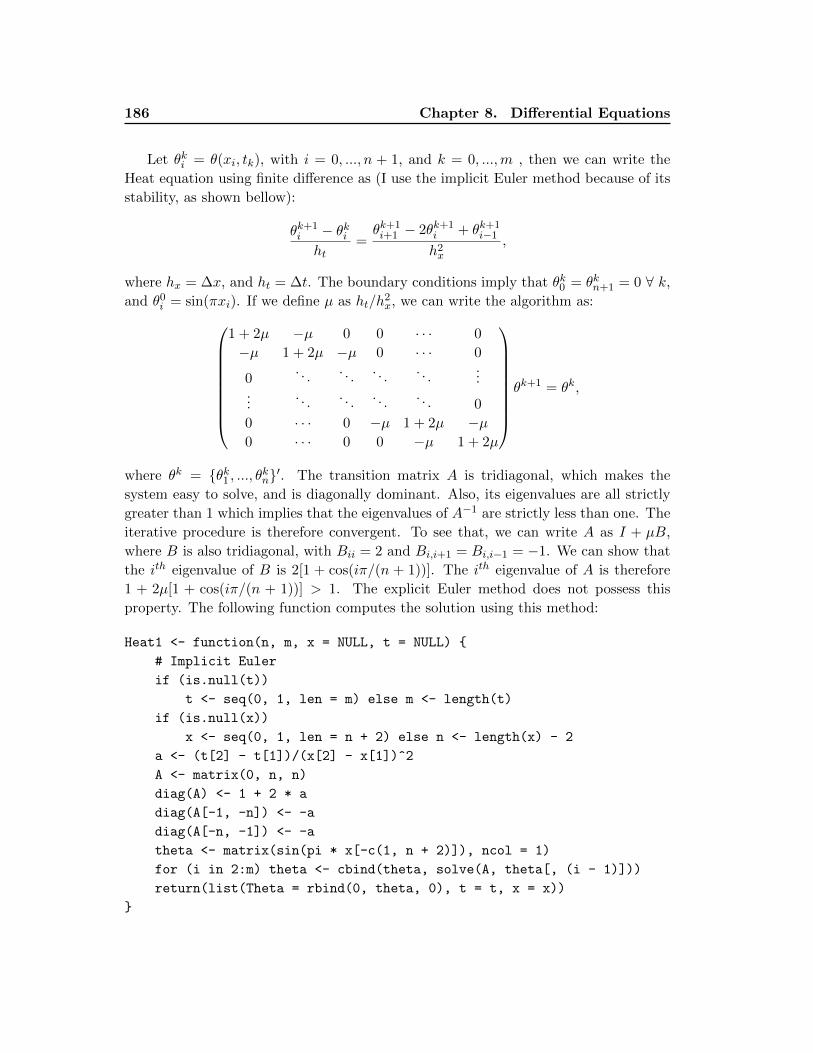
186 Chapter 8. Differential Equations
Let θki = θ(xi, tk), with i = 0, ..., n + 1, and k = 0, ...,m , then we can write the
Heat equation using finite difference as (I use the implicit Euler method because of its
stability, as shown bellow):
θk+1i − θkiht
=θk+1i+1 − 2θk+1
i + θk+1i−1
h2x,
where hx = ∆x, and ht = ∆t. The boundary conditions imply that θk0 = θkn+1 = 0 ∀ k,
and θ0i = sin(πxi). If we define µ as ht/h2x, we can write the algorithm as:
1 + 2µ −µ 0 0 · · · 0
−µ 1 + 2µ −µ 0 · · · 0
0. . .
. . .. . .
. . ....
.... . .
. . .. . .
. . . 0
0 · · · 0 −µ 1 + 2µ −µ0 · · · 0 0 −µ 1 + 2µ
θk+1 = θk,
where θk = {θk1 , ..., θkn}′. The transition matrix A is tridiagonal, which makes the
system easy to solve, and is diagonally dominant. Also, its eigenvalues are all strictly
greater than 1 which implies that the eigenvalues of A−1 are strictly less than one. The
iterative procedure is therefore convergent. To see that, we can write A as I + µB,
where B is also tridiagonal, with Bii = 2 and Bi,i+1 = Bi,i−1 = −1. We can show that
the ith eigenvalue of B is 2[1 + cos(iπ/(n + 1))]. The ith eigenvalue of A is therefore
1 + 2µ[1 + cos(iπ/(n + 1))] > 1. The explicit Euler method does not possess this
property. The following function computes the solution using this method:
Heat1 <- function(n, m, x = NULL, t = NULL) {
# Implicit Euler
if (is.null(t))
t <- seq(0, 1, len = m) else m <- length(t)
if (is.null(x))
x <- seq(0, 1, len = n + 2) else n <- length(x) - 2
a <- (t[2] - t[1])/(x[2] - x[1])^2
A <- matrix(0, n, n)
diag(A) <- 1 + 2 * a
diag(A[-1, -n]) <- -a
diag(A[-n, -1]) <- -a
theta <- matrix(sin(pi * x[-c(1, n + 2)]), ncol = 1)
for (i in 2:m) theta <- cbind(theta, solve(A, theta[, (i - 1)]))
return(list(Theta = rbind(0, theta, 0), t = t, x = x))
}
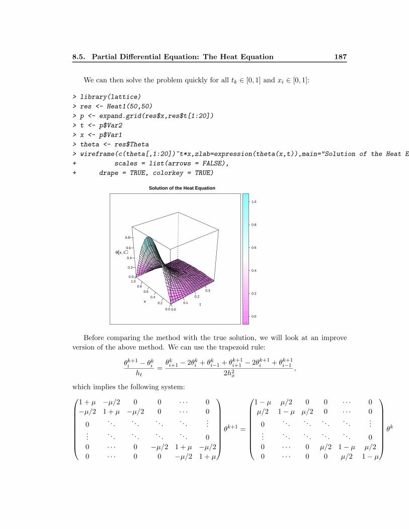
8.5. Partial Differential Equation: The Heat Equation 187
We can then solve the problem quickly for all tk ∈ [0, 1] and xi ∈ [0, 1]:
> library(lattice)
> res <- Heat1(50,50)
> p <- expand.grid(res$x,res$t[1:20])
> t <- p$Var2
> x <- p$Var1
> theta <- res$Theta
> wireframe(c(theta[,1:20])~t*x,zlab=expression(theta(x,t)),main="Solution of the Heat Equation",
+ scales = list(arrows = FALSE),
+ drape = TRUE, colorkey = TRUE)
Solution of the Heat Equation
0.0
0.1
0.2
0.3
0.0
0.2
0.4
0.6
0.8
1.00.0
0.2
0.4
0.6
0.8
tx
θ(x, t)
0.0
0.2
0.4
0.6
0.8
1.0
Before comparing the method with the true solution, we will look at an improve
version of the above method. We can use the trapezoid rule:
θk+1i − θkiht
=θki+1 − 2θki + θki−1 + θk+1
i+1 − 2θk+1i + θk+1
i−12h2x
,
which implies the following system:
1 + µ −µ/2 0 0 · · · 0
−µ/2 1 + µ −µ/2 0 · · · 0
0. . .
. . .. . .
. . ....
.... . .
. . .. . .
. . . 0
0 · · · 0 −µ/2 1 + µ −µ/20 · · · 0 0 −µ/2 1 + µ
θk+1 =
1− µ µ/2 0 0 · · · 0
µ/2 1− µ µ/2 0 · · · 0
0. . .
. . .. . .
. . ....
.... . .
. . .. . .
. . . 0
0 · · · 0 µ/2 1− µ µ/2
0 · · · 0 0 µ/2 1− µ
θk
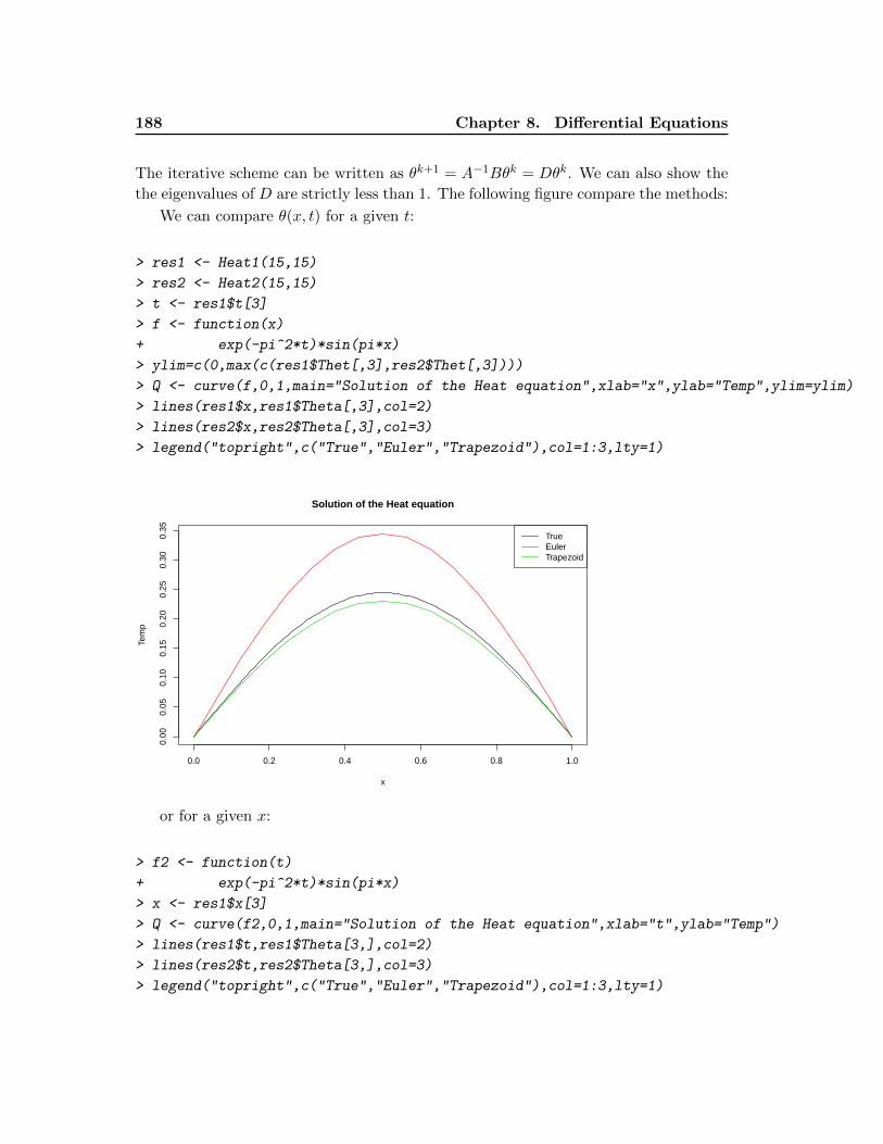
188 Chapter 8. Differential Equations
The iterative scheme can be written as θk+1 = A−1Bθk = Dθk. We can also show the
the eigenvalues of D are strictly less than 1. The following figure compare the methods:
We can compare θ(x, t) for a given t:
> res1 <- Heat1(15,15)
> res2 <- Heat2(15,15)
> t <- res1$t[3]
> f <- function(x)
+ exp(-pi^2*t)*sin(pi*x)
> ylim=c(0,max(c(res1$Thet[,3],res2$Thet[,3])))
> Q <- curve(f,0,1,main="Solution of the Heat equation",xlab="x",ylab="Temp",ylim=ylim)
> lines(res1$x,res1$Theta[,3],col=2)
> lines(res2$x,res2$Theta[,3],col=3)
> legend("topright",c("True","Euler","Trapezoid"),col=1:3,lty=1)
0.0 0.2 0.4 0.6 0.8 1.0
0.00
0.05
0.10
0.15
0.20
0.25
0.30
0.35
Solution of the Heat equation
x
Tem
p
TrueEulerTrapezoid
or for a given x:
> f2 <- function(t)
+ exp(-pi^2*t)*sin(pi*x)
> x <- res1$x[3]
> Q <- curve(f2,0,1,main="Solution of the Heat equation",xlab="t",ylab="Temp")
> lines(res1$t,res1$Theta[3,],col=2)
> lines(res2$t,res2$Theta[3,],col=3)
> legend("topright",c("True","Euler","Trapezoid"),col=1:3,lty=1)
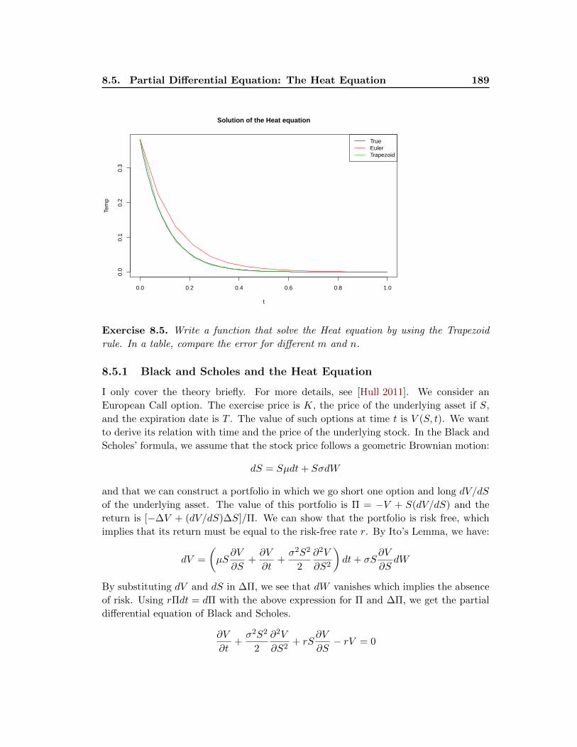
8.5. Partial Differential Equation: The Heat Equation 189
0.0 0.2 0.4 0.6 0.8 1.0
0.0
0.1
0.2
0.3
Solution of the Heat equation
t
Tem
p
TrueEulerTrapezoid
Exercise 8.5. Write a function that solve the Heat equation by using the Trapezoid
rule. In a table, compare the error for different m and n.
8.5.1 Black and Scholes and the Heat Equation
I only cover the theory briefly. For more details, see [Hull 2011]. We consider an
European Call option. The exercise price is K, the price of the underlying asset if S,
and the expiration date is T . The value of such options at time t is V (S, t). We want
to derive its relation with time and the price of the underlying stock. In the Black and
Scholes’ formula, we assume that the stock price follows a geometric Brownian motion:
dS = Sµdt+ SσdW
and that we can construct a portfolio in which we go short one option and long dV/dS
of the underlying asset. The value of this portfolio is Π = −V + S(dV/dS) and the
return is [−∆V + (dV/dS)∆S]/Π. We can show that the portfolio is risk free, which
implies that its return must be equal to the risk-free rate r. By Ito’s Lemma, we have:
dV =
(µS
∂V
∂S+∂V
∂t+σ2S2
2
∂2V
∂S2
)dt+ σS
∂V
∂SdW
By substituting dV and dS in ∆Π, we see that dW vanishes which implies the absence
of risk. Using rΠdt = dΠ with the above expression for Π and ∆Π, we get the partial
differential equation of Black and Scholes.
∂V
∂t+σ2S2
2
∂2V
∂S2+ rS
∂V
∂S− rV = 0
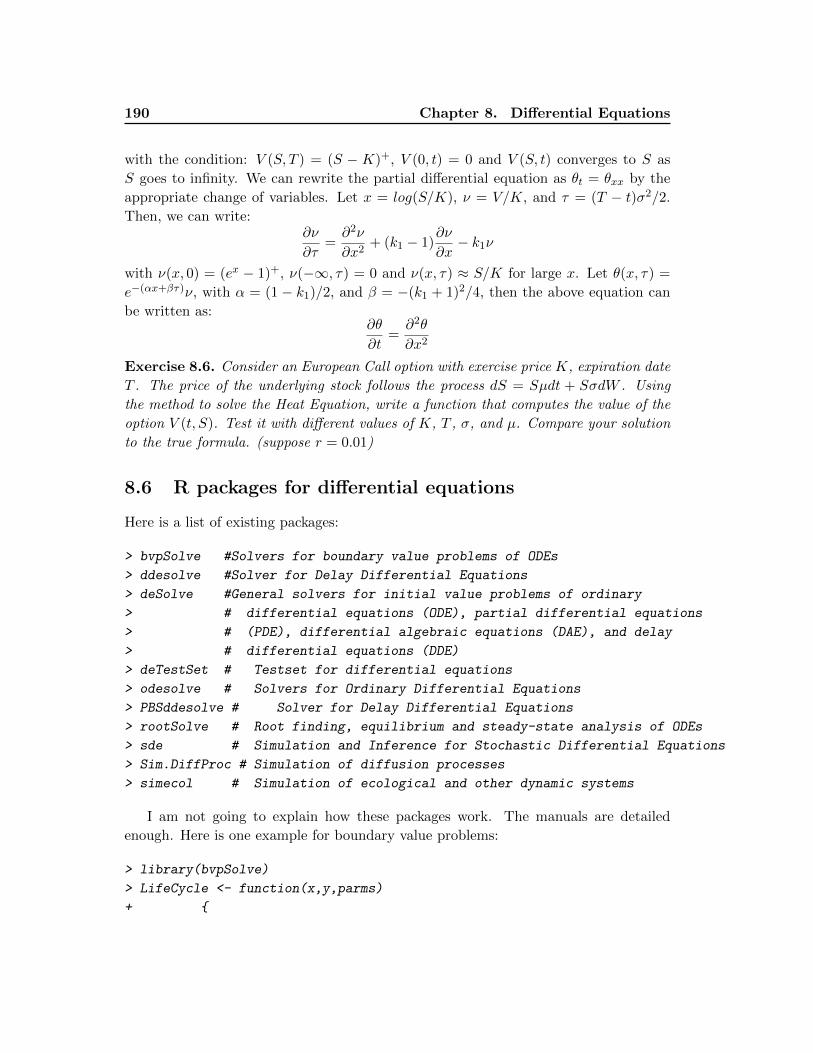
190 Chapter 8. Differential Equations
with the condition: V (S, T ) = (S − K)+, V (0, t) = 0 and V (S, t) converges to S as
S goes to infinity. We can rewrite the partial differential equation as θt = θxx by the
appropriate change of variables. Let x = log(S/K), ν = V/K, and τ = (T − t)σ2/2.
Then, we can write:∂ν
∂τ=∂2ν
∂x2+ (k1 − 1)
∂ν
∂x− k1ν
with ν(x, 0) = (ex − 1)+, ν(−∞, τ) = 0 and ν(x, τ) ≈ S/K for large x. Let θ(x, τ) =
e−(αx+βτ)ν, with α = (1 − k1)/2, and β = −(k1 + 1)2/4, then the above equation can
be written as:∂θ
∂t=∂2θ
∂x2
Exercise 8.6. Consider an European Call option with exercise price K, expiration date
T . The price of the underlying stock follows the process dS = Sµdt + SσdW . Using
the method to solve the Heat Equation, write a function that computes the value of the
option V (t, S). Test it with different values of K, T , σ, and µ. Compare your solution
to the true formula. (suppose r = 0.01)
8.6 R packages for differential equations
Here is a list of existing packages:
> bvpSolve #Solvers for boundary value problems of ODEs
> ddesolve #Solver for Delay Differential Equations
> deSolve #General solvers for initial value problems of ordinary
> # differential equations (ODE), partial differential equations
> # (PDE), differential algebraic equations (DAE), and delay
> # differential equations (DDE)
> deTestSet # Testset for differential equations
> odesolve # Solvers for Ordinary Differential Equations
> PBSddesolve # Solver for Delay Differential Equations
> rootSolve # Root finding, equilibrium and steady-state analysis of ODEs
> sde # Simulation and Inference for Stochastic Differential Equations
> Sim.DiffProc # Simulation of diffusion processes
> simecol # Simulation of ecological and other dynamic systems
I am not going to explain how these packages work. The manuals are detailed
enough. Here is one example for boundary value problems:
> library(bvpSolve)
> LifeCycle <- function(x,y,parms)
+ {
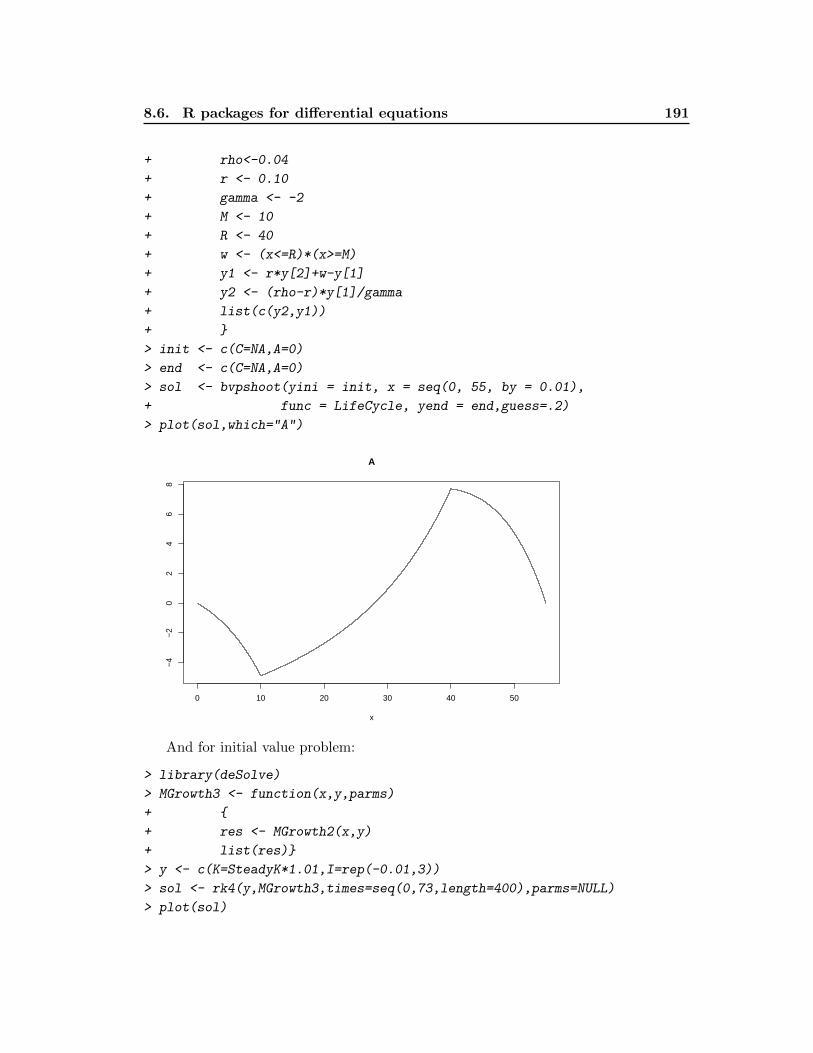
8.6. R packages for differential equations 191
+ rho<-0.04
+ r <- 0.10
+ gamma <- -2
+ M <- 10
+ R <- 40
+ w <- (x<=R)*(x>=M)
+ y1 <- r*y[2]+w-y[1]
+ y2 <- (rho-r)*y[1]/gamma
+ list(c(y2,y1))
+ }
> init <- c(C=NA,A=0)
> end <- c(C=NA,A=0)
> sol <- bvpshoot(yini = init, x = seq(0, 55, by = 0.01),
+ func = LifeCycle, yend = end,guess=.2)
> plot(sol,which="A")
0 10 20 30 40 50
−4
−2
02
46
8
A
x
And for initial value problem:
> library(deSolve)
> MGrowth3 <- function(x,y,parms)
+ {
+ res <- MGrowth2(x,y)
+ list(res)}
> y <- c(K=SteadyK*1.01,I=rep(-0.01,3))
> sol <- rk4(y,MGrowth3,times=seq(0,73,length=400),parms=NULL)
> plot(sol)
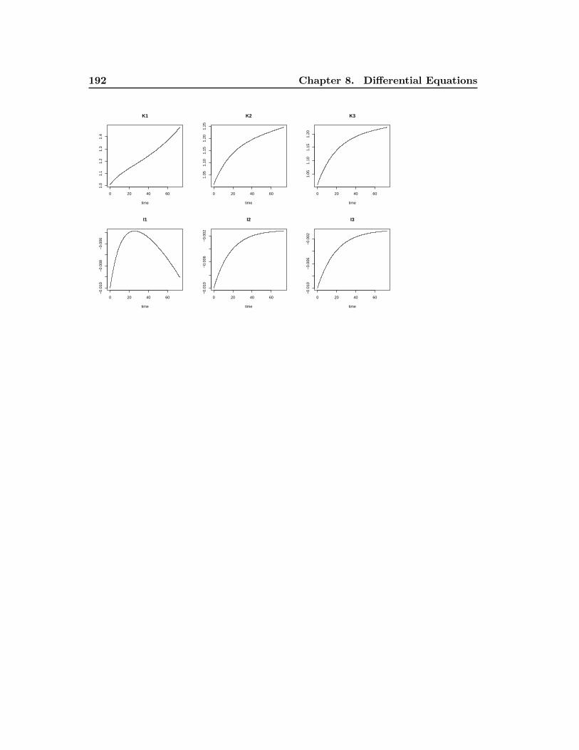
192 Chapter 8. Differential Equations
0 20 40 60
1.0
1.1
1.2
1.3
1.4
K1
time
0 20 40 60
1.05
1.10
1.15
1.20
1.25
K2
time
0 20 40 60
1.05
1.10
1.15
1.20
K3
time
0 20 40 60
−0.
010
−0.
008
−0.
006
I1
time
0 20 40 60
−0.
010
−0.
006
−0.
002
I2
time
0 20 40 60
−0.
010
−0.
006
−0.
002
I3
time
Appendix A
Solution to some Problems
A.1 Chapter 1
Exercise 1.2. In order to do the exercise, you will need to load the data file ”Pri-
ceIndex.rda”, in which you’ll find seven vectors of price index: all, Car, Clothing,
Electricity, Food, NatGas and Gasoline. All vectors are monthly time series going from
January 1949 to September 2011. This exercise makes you use what we have covered
above and more. You may need to use Google, help() or help.search(). That is where
the fun begins
1. Collect the data in a matrix of class ”ts” with the correct starting date and fre-
quency. You can then plot the data and compare the inflation of different items.
> load("../../data/PriceIndex.rda")
> Nvar <- objects() # I only have the loaded variables in the workspace
> CPI <- get(Nvar[1]) # get the variable from its name
> for (i in 2:length(Nvar))
+ CPI <- cbind(CPI,get(Nvar[i]))
> colnames(CPI) <- Nvar
> CPI <- ts(CPI,freq=12,start=c(1949,1))
> INF <- diff(CPI)/lag(CPI,-1)
> colnames(INF) <- colnames(CPI)
> plot(INF, main="Inflation using different price indices")
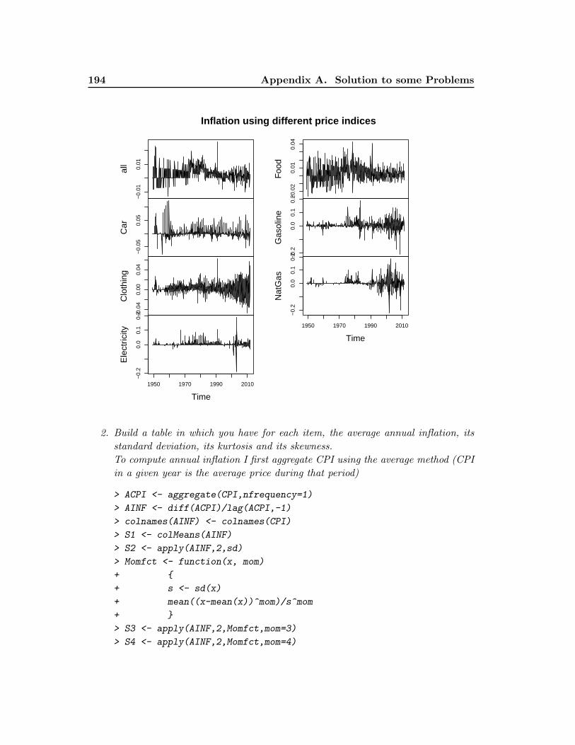
194 Appendix A. Solution to some Problems
−0.
010.
01
all
−0.
050.
05
Car
−0.
040.
000.
04
Clo
thin
g
−0.
20.
00.
10.
2
1950 1970 1990 2010
Ele
ctric
ity
Time
−0.
020.
010.
04
Foo
d
−0.
20.
00.
10.
2
Gas
olin
e
−0.
20.
00.
10.
2
1950 1970 1990 2010
Nat
Gas
Time
Inflation using different price indices
2. Build a table in which you have for each item, the average annual inflation, its
standard deviation, its kurtosis and its skewness.
To compute annual inflation I first aggregate CPI using the average method (CPI
in a given year is the average price during that period)
> ACPI <- aggregate(CPI,nfrequency=1)
> AINF <- diff(ACPI)/lag(ACPI,-1)
> colnames(AINF) <- colnames(CPI)
> S1 <- colMeans(AINF)
> S2 <- apply(AINF,2,sd)
> Momfct <- function(x, mom)
+ {
+ s <- sd(x)
+ mean((x-mean(x))^mom)/s^mom
+ }
> S3 <- apply(AINF,2,Momfct,mom=3)
> S4 <- apply(AINF,2,Momfct,mom=4)
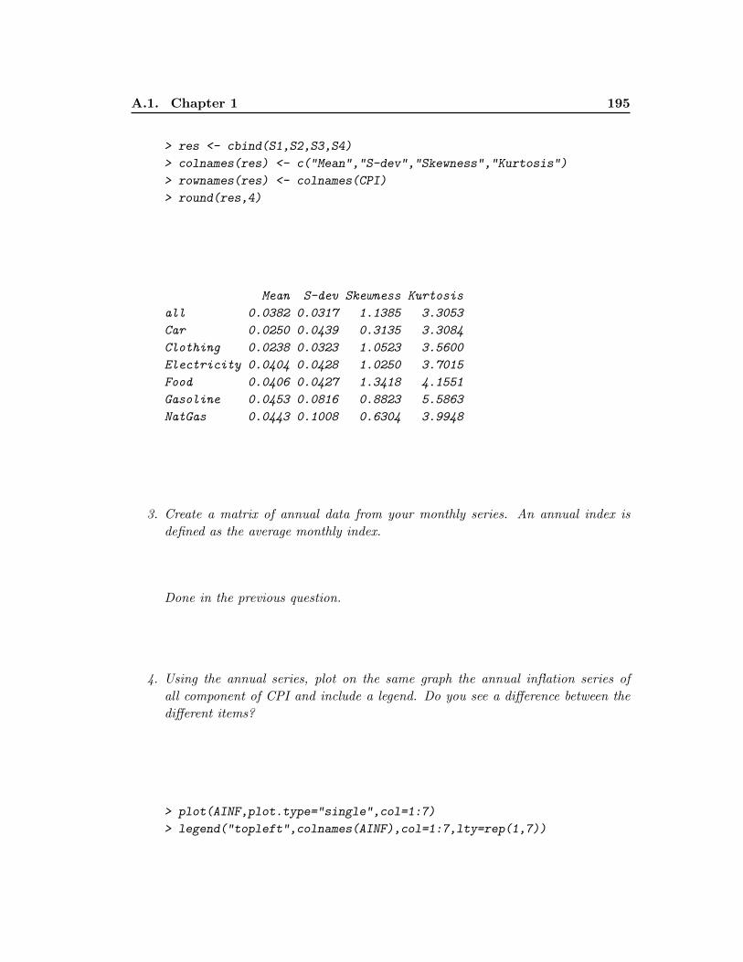
A.1. Chapter 1 195
> res <- cbind(S1,S2,S3,S4)
> colnames(res) <- c("Mean","S-dev","Skewness","Kurtosis")
> rownames(res) <- colnames(CPI)
> round(res,4)
Mean S-dev Skewness Kurtosis
all 0.0382 0.0317 1.1385 3.3053
Car 0.0250 0.0439 0.3135 3.3084
Clothing 0.0238 0.0323 1.0523 3.5600
Electricity 0.0404 0.0428 1.0250 3.7015
Food 0.0406 0.0427 1.3418 4.1551
Gasoline 0.0453 0.0816 0.8823 5.5863
NatGas 0.0443 0.1008 0.6304 3.9948
3. Create a matrix of annual data from your monthly series. An annual index is
defined as the average monthly index.
Done in the previous question.
4. Using the annual series, plot on the same graph the annual inflation series of
all component of CPI and include a legend. Do you see a difference between the
different items?
> plot(AINF,plot.type="single",col=1:7)
> legend("topleft",colnames(AINF),col=1:7,lty=rep(1,7))
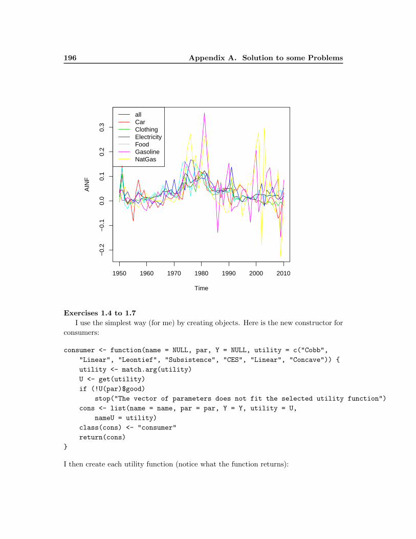
196 Appendix A. Solution to some Problems
Time
AIN
F
1950 1960 1970 1980 1990 2000 2010
−0.
2−
0.1
0.0
0.1
0.2
0.3
allCarClothingElectricityFoodGasolineNatGas
Exercises 1.4 to 1.7
I use the simplest way (for me) by creating objects. Here is the new constructor for
consumers:
consumer <- function(name = NULL, par, Y = NULL, utility = c("Cobb",
"Linear", "Leontief", "Subsistence", "CES", "Linear", "Concave")) {
utility <- match.arg(utility)
U <- get(utility)
if (!U(par)$good)
stop("The vector of parameters does not fit the selected utility function")
cons <- list(name = name, par = par, Y = Y, utility = U,
nameU = utility)
class(cons) <- "consumer"
return(cons)
}
I then create each utility function (notice what the function returns):
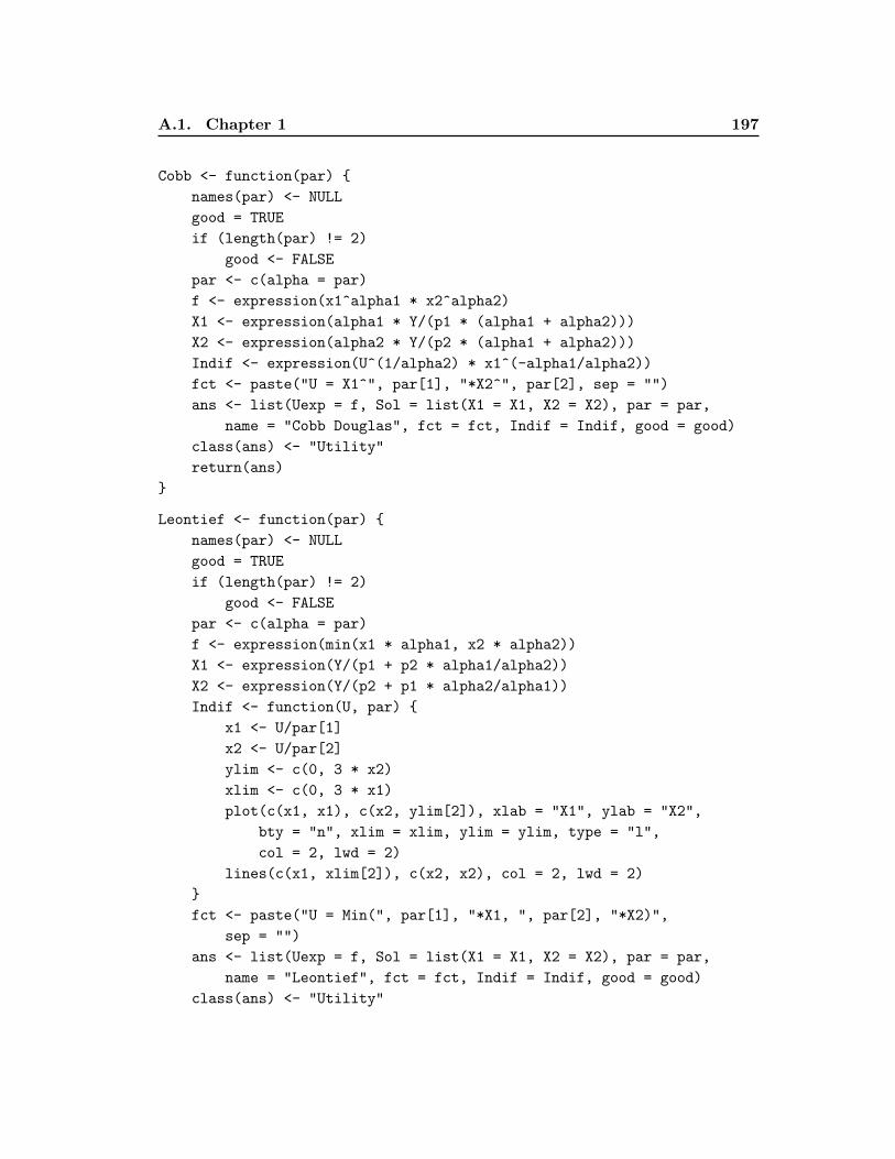
A.1. Chapter 1 197
Cobb <- function(par) {
names(par) <- NULL
good = TRUE
if (length(par) != 2)
good <- FALSE
par <- c(alpha = par)
f <- expression(x1^alpha1 * x2^alpha2)
X1 <- expression(alpha1 * Y/(p1 * (alpha1 + alpha2)))
X2 <- expression(alpha2 * Y/(p2 * (alpha1 + alpha2)))
Indif <- expression(U^(1/alpha2) * x1^(-alpha1/alpha2))
fct <- paste("U = X1^", par[1], "*X2^", par[2], sep = "")
ans <- list(Uexp = f, Sol = list(X1 = X1, X2 = X2), par = par,
name = "Cobb Douglas", fct = fct, Indif = Indif, good = good)
class(ans) <- "Utility"
return(ans)
}
Leontief <- function(par) {
names(par) <- NULL
good = TRUE
if (length(par) != 2)
good <- FALSE
par <- c(alpha = par)
f <- expression(min(x1 * alpha1, x2 * alpha2))
X1 <- expression(Y/(p1 + p2 * alpha1/alpha2))
X2 <- expression(Y/(p2 + p1 * alpha2/alpha1))
Indif <- function(U, par) {
x1 <- U/par[1]
x2 <- U/par[2]
ylim <- c(0, 3 * x2)
xlim <- c(0, 3 * x1)
plot(c(x1, x1), c(x2, ylim[2]), xlab = "X1", ylab = "X2",
bty = "n", xlim = xlim, ylim = ylim, type = "l",
col = 2, lwd = 2)
lines(c(x1, xlim[2]), c(x2, x2), col = 2, lwd = 2)
}
fct <- paste("U = Min(", par[1], "*X1, ", par[2], "*X2)",
sep = "")
ans <- list(Uexp = f, Sol = list(X1 = X1, X2 = X2), par = par,
name = "Leontief", fct = fct, Indif = Indif, good = good)
class(ans) <- "Utility"
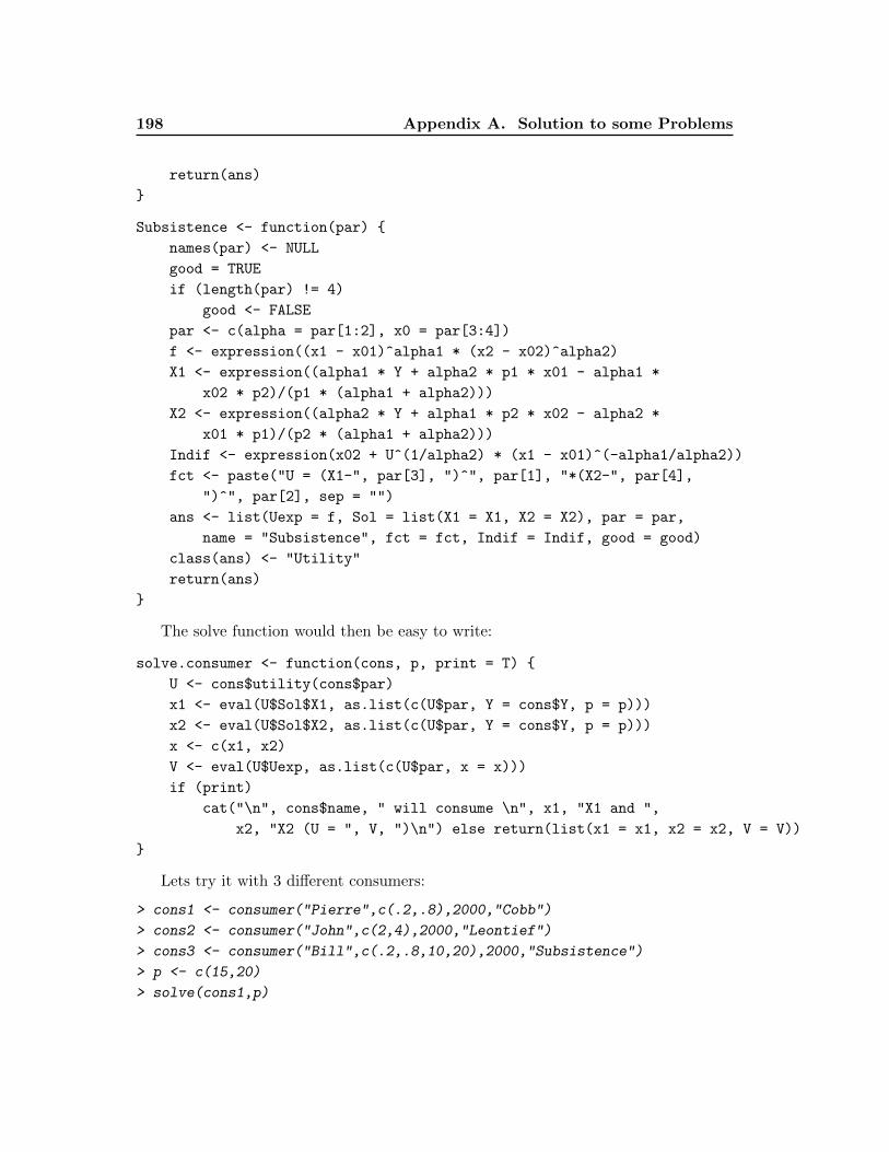
198 Appendix A. Solution to some Problems
return(ans)
}
Subsistence <- function(par) {
names(par) <- NULL
good = TRUE
if (length(par) != 4)
good <- FALSE
par <- c(alpha = par[1:2], x0 = par[3:4])
f <- expression((x1 - x01)^alpha1 * (x2 - x02)^alpha2)
X1 <- expression((alpha1 * Y + alpha2 * p1 * x01 - alpha1 *
x02 * p2)/(p1 * (alpha1 + alpha2)))
X2 <- expression((alpha2 * Y + alpha1 * p2 * x02 - alpha2 *
x01 * p1)/(p2 * (alpha1 + alpha2)))
Indif <- expression(x02 + U^(1/alpha2) * (x1 - x01)^(-alpha1/alpha2))
fct <- paste("U = (X1-", par[3], ")^", par[1], "*(X2-", par[4],
")^", par[2], sep = "")
ans <- list(Uexp = f, Sol = list(X1 = X1, X2 = X2), par = par,
name = "Subsistence", fct = fct, Indif = Indif, good = good)
class(ans) <- "Utility"
return(ans)
}
The solve function would then be easy to write:
solve.consumer <- function(cons, p, print = T) {
U <- cons$utility(cons$par)
x1 <- eval(U$Sol$X1, as.list(c(U$par, Y = cons$Y, p = p)))
x2 <- eval(U$Sol$X2, as.list(c(U$par, Y = cons$Y, p = p)))
x <- c(x1, x2)
V <- eval(U$Uexp, as.list(c(U$par, x = x)))
if (print)
cat("\n", cons$name, " will consume \n", x1, "X1 and ",
x2, "X2 (U = ", V, ")\n") else return(list(x1 = x1, x2 = x2, V = V))
}
Lets try it with 3 different consumers:
> cons1 <- consumer("Pierre",c(.2,.8),2000,"Cobb")
> cons2 <- consumer("John",c(2,4),2000,"Leontief")
> cons3 <- consumer("Bill",c(.2,.8,10,20),2000,"Subsistence")
> p <- c(15,20)
> solve(cons1,p)
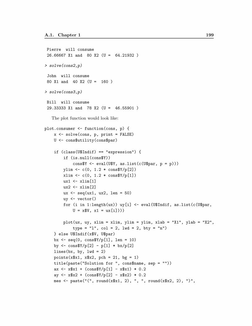
A.1. Chapter 1 199
Pierre will consume
26.66667 X1 and 80 X2 (U = 64.21932 )
> solve(cons2,p)
John will consume
80 X1 and 40 X2 (U = 160 )
> solve(cons3,p)
Bill will consume
29.33333 X1 and 78 X2 (U = 46.55901 )
The plot function would look like:
plot.consumer <- function(cons, p) {
x <- solve(cons, p, print = FALSE)
U <- cons$utility(cons$par)
if (class(U$Indif) == "expression") {
if (is.null(cons$Y))
cons$Y <- eval(U$Y, as.list(c(U$par, p = p)))
ylim <- c(0, 1.2 * cons$Y/p[2])
xlim <- c(0, 1.2 * cons$Y/p[1])
ux1 <- xlim[1]
ux2 <- xlim[2]
ux <- seq(ux1, ux2, len = 50)
uy <- vector()
for (i in 1:length(ux)) uy[i] <- eval(U$Indif, as.list(c(U$par,
U = x$V, x1 = ux[i])))
plot(ux, uy, xlim = xlim, ylim = ylim, xlab = "X1", ylab = "X2",
type = "l", col = 2, lwd = 2, bty = "n")
} else U$Indif(x$V, U$par)
bx <- seq(0, cons$Y/p[1], len = 10)
by <- cons$Y/p[2] - p[1] * bx/p[2]
lines(bx, by, lwd = 2)
points(x$x1, x$x2, pch = 21, bg = 1)
title(paste("Solution for ", cons$name, sep = ""))
ax <- x$x1 + (cons$Y/p[1] - x$x1) * 0.2
ay <- x$x2 + (cons$Y/p[2] - x$x2) * 0.2
mes <- paste("(", round(x$x1, 2), ", ", round(x$x2, 2), ")",
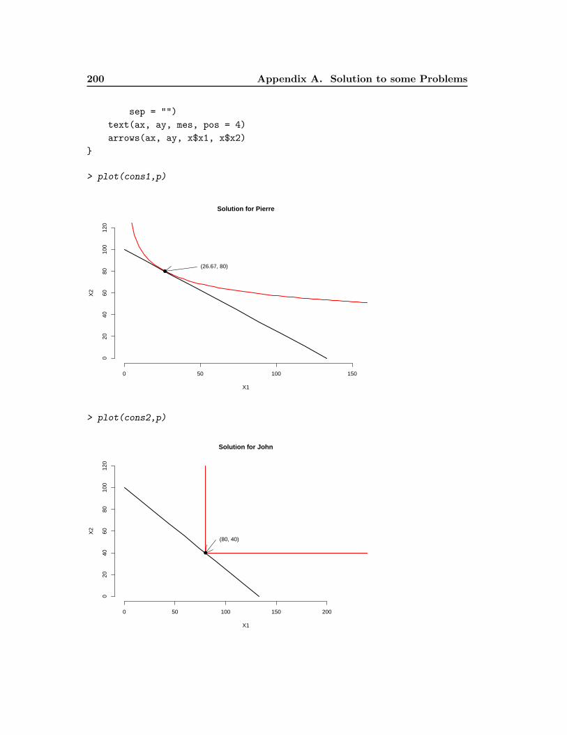
200 Appendix A. Solution to some Problems
sep = "")
text(ax, ay, mes, pos = 4)
arrows(ax, ay, x$x1, x$x2)
}
> plot(cons1,p)
0 50 100 150
020
4060
8010
012
0
X1
X2
●
Solution for Pierre
(26.67, 80)
> plot(cons2,p)
0 50 100 150 200
020
4060
8010
012
0
X1
X2
●
Solution for John
(80, 40)
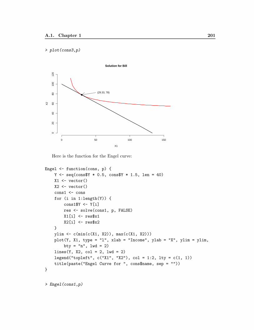
A.1. Chapter 1 201
> plot(cons3,p)
0 50 100 150
020
4060
8010
012
0
X1
X2
●
Solution for Bill
(29.33, 78)
Here is the function for the Engel curve:
Engel <- function(cons, p) {
Y <- seq(cons$Y * 0.5, cons$Y * 1.5, len = 40)
X1 <- vector()
X2 <- vector()
cons1 <- cons
for (i in 1:length(Y)) {
cons1$Y <- Y[i]
res <- solve(cons1, p, FALSE)
X1[i] <- res$x1
X2[i] <- res$x2
}
ylim <- c(min(c(X1, X2)), max(c(X1, X2)))
plot(Y, X1, type = "l", xlab = "Income", ylab = "X", ylim = ylim,
bty = "n", lwd = 2)
lines(Y, X2, col = 2, lwd = 2)
legend("topleft", c("X1", "X2"), col = 1:2, lty = c(1, 1))
title(paste("Engel Curve for ", cons$name, sep = ""))
}
> Engel(cons1,p)
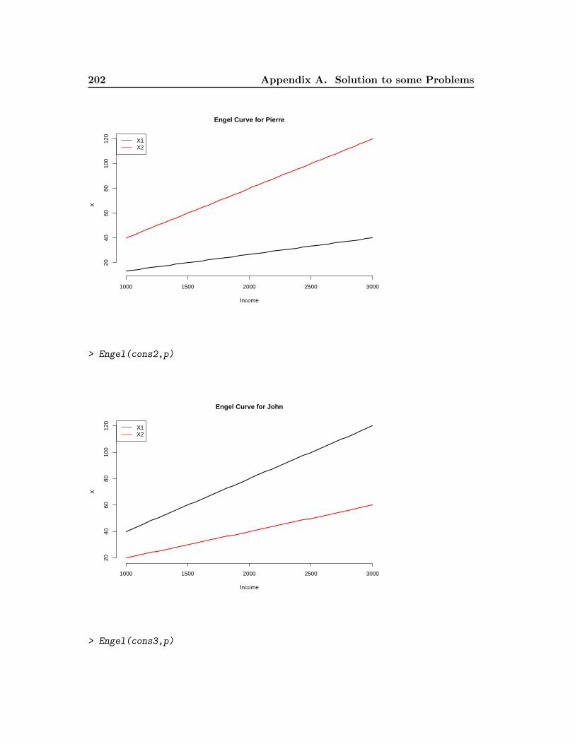
202 Appendix A. Solution to some Problems
1000 1500 2000 2500 3000
2040
6080
100
120
Income
X
X1X2
Engel Curve for Pierre
> Engel(cons2,p)
1000 1500 2000 2500 3000
2040
6080
100
120
Income
X
X1X2
Engel Curve for John
> Engel(cons3,p)
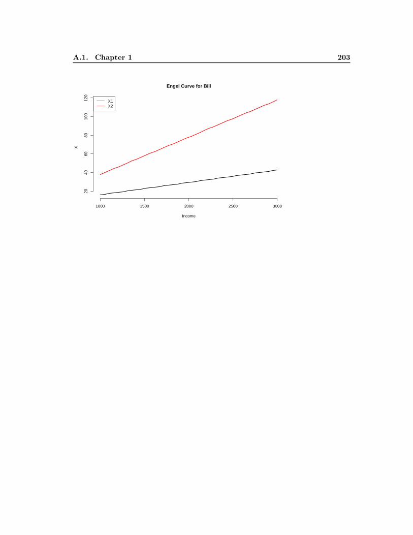
A.1. Chapter 1 203
1000 1500 2000 2500 3000
2040
6080
100
120
Income
X
X1X2
Engel Curve for Bill

Bibliography
[Genz et al. 2011] A. Genz, F. Bretz, T. Miwa, X. Mi, F Leisch, F. Scheipl and
T. Hothorn. mvtnorm: Multivariate Normal and t Distributions. R Foundation
for Statistical Computing, Vienna, Austria, 2011. R package version 0.9-9991.
(Cited on page 6.)
[Goldberg 1991] D. Goldberg. What every Computer Scientist Should Know About
Floating-Point Arithmetic. ACM Computing Surveys, vol. 23, no. 1, pages 5–
48, 1991. (Cited on page 49.)
[Golub & Ortega 1992] G.H. Golub and J.M. Ortega. Scientific computing and differ-
ential equations. Academic Press, 1992. (Cited on page 185.)
[Hasselman 2012] Berend Hasselman. nleqslv: Solve systems of non linear equations,
2012. R package version 1.9.3. (Cited on page 133.)
[Hull 2011] J.C. Hull. Options, futures, and other derivatives. Prentice Hall, 2011.
(Cited on page 189.)
[Judd 1998] K.L. Judd. Numerical methods in economics. The MIT Press, 1998. (Cited
on page 57.)
[Press et al. 2007] W.H. Press, S.A. Teukolsky, W.T. Vetterling and B.P. Flannery.
Numerical recipes, third edition. Cambridge University Press, 2007. (Cited on
page 108.)
[Smyth et al. 2011] Gordon Smyth, Yifang Hu, Peter Dunn and Belinda Phipson. stat-
mod: Statistical Modeling, 2011. R package version 1.4.14. (Cited on page 143.)
[Spence 1974] M.A. Spence. Competitive and optimal responses to signals: An analysis
of efficiency and distribution. Journal of Economic Theory, vol. 7, no. 3, pages
296–332, 1974. (Cited on page 165.)
[Urbanek 2011] Simon Urbanek. multicore: Parallel processing of R code on machines
with multiple cores or CPUs, 2011. R package version 0.1-7. (Cited on page 46.)
[Wuertz et al. 2009] Diethelm Wuertz, many others and see the SOURCE file. fUni-
tRoots: Trends and Unit Roots, 2009. R package version 2100.76. (Cited on
page 13.)


![Lectures on holographic methods for condensed matter physics · arXiv:0903.3246 [hep-th] Lectures on holographic methods for condensed matter physics Sean A. Hartnoll Je erson Physical](https://static.documents.pub/doc/80x56/5b717a757f8b9ae54f8b7fd5/lectures-on-holographic-methods-for-condensed-matter-physics-arxiv09033246.jpg)
