1

Statistics for Economists Lectures 5 & 6

Asrat Temesgen

Stockholm University

2

Chapter 3- Continuous Distributions

3.1. Continuous-Type data

If measurements could come from an interval of possible outcomes, we call

them continuous-type data.

The following guidelines and terminology will be used to group continuous type

data into classes of equal length:

1. Determine the maximum & minimum observations. The Range is R =

maximum – minimum.

2. In general, select from k=5 to k=20 classes, which are usually non

overlapping intervals of equal length. These classes should cover the

interval from the minimum to the maximum.

3. Each interval begins and ends halfway between two possible values of

the measurements, which have been rounded off to a given number of

decimal places.

4. The first interval should begin about as much below the smallest value

as the last interval ends above the largest.

5. The intervals are called class intervals and the boundaries are called

class boundaries or cut points. We shall denote these k class intervals by

(C0, C1), (C1,C2),…,(Ck-1,Ck).

6. The class limits are the smallest and the largest possible observed values

in a class.

7. The class mark is the midpoint of a class.

A frequency table is constructed that lists the class intervals, the class limits, a

tabulation of the measurements in the various classes, the frequency fi of each

class, and the class marks.

3

The function defined by

is called

a relative frequency histogram or density histogram, where fi is the frequency of

the ith class and n is the total number of observations.

Example 3.1-1: The weights in grams of 40 miniature Baby Ruth candy bars,

with the weights ordered, are given in table 3.1-1.

Table 3.1-1: Candy Bar weights

20.5 20.7 20.8 21.0 21.0 21.4 21.5 22.0 22.1 22.5

22.6 22.6 22.7 22.7 22.9 22.9 23.1 23.3 23.4 23.5

23.6 23.6 23.6 23.9 24.1 24.3 24.5 24.5 24.8 24.8

24.9 24.9 25.1 25.1 25.2 25.6 25.8 25.9 26.1 26.7

We shall group these data and then construct a histogram to visualize the

distribution of weights. The range of the data is R=26.7-20.5=6.2. The interval

(20.5, 26.7) could be covered with k=8 classes of width 0.8 or with k=9 classes

of width 0.7. (There are other possibilities.) We shall use k=7 classes of width

0.9. The first class interval will be (20.45, 21.35) and the last class interval will

be (25.85, 26.75). The data are grouped in Table 3.1-2.

Table 3.1-2: Frequency Table of Candy Bar Weighs

Class interval Class

limits

Tabulation Frequency

(fi)

h(x) Class

Marks (ui)

(20.45,21.35) 20.5 - 21.3 |||| 5 5/36 20.9

(21.35,22.25) 21.4 - 22.2 |||| 4 4/36 21.8

(22.25,23.15) 22.3-23.1 |||| ||| 8 8/36 22.7

(23.15,24.05) 23.2-24.0 |||| || 7 7/36 23.6

(24.05,24.95) 24.1-24.9 |||| ||| 8 8/36 24.5

(24.95,25.85) 25.0-25.8 |||| 5 5/36 25.4

(25.85,26.75) 25.9-26.7 ||| 3 3/36 26.3

4

A relative frequency histogram of these data is given in Figure 3.1-1.

Note that the total area of this histogram is equal to 1.

Notes

1. Given a set of measurements, the sample mean is the center of the data

such that the deviations from that center sum to zero; that is,

The sample standard devistion gives a measure of how spread out

the data are from the sample mean.

2. Let x1, x2,…,xn have a sample mean and sample standard deviation s. If

the histogram of these data is “bell shaped”, then

a) approximately 68% of the data are in the interval (

b) approximately 95% of the data are in the interval

c) approximately 99.7% of the data are in the interval

3. For grouped data, we can obtain close approximations of the mean and

variance using the class marks weighted with their respective frequencies.

i.e. we have

0

0,05

0,1

0,15

0,2

0,25

0,3

20,9 21,8 22,7 23,6 24,5 25,4 26,3

Figure 3.1-1: Relative frequency histogram of weights of Candy bard

Series 1

5

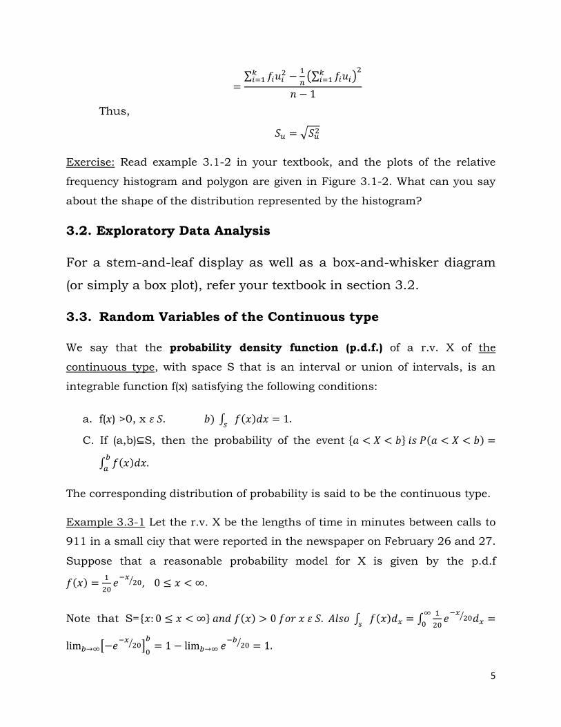
Thus,

Exercise: Read example 3.1-2 in your textbook, and the plots of the relative

frequency histogram and polygon are given in Figure 3.1-2. What can you say

about the shape of the distribution represented by the histogram?

3.2. Exploratory Data Analysis

For a stem-and-leaf display as well as a box-and-whisker diagram

(or simply a box plot), refer your textbook in section 3.2.

3.3. Random Variables of the Continuous type

We say that the probability density function (p.d.f.) of a r.v. X of the

continuous type, with space S that is an interval or union of intervals, is an

integrable function f(x) satisfying the following conditions:

a. f( ) >0, x

C. If (a,b)⊆S, then the probability of the event

The corresponding distribution of probability is said to be the continuous type.

Example 3.3-1 Let the r.v. X be the lengths of time in minutes between calls to

911 in a small city that were reported in the newspaper on February 26 and 27.

Suppose that a reasonable probability model for X is given by the p.d.f

.

Note that S=

6

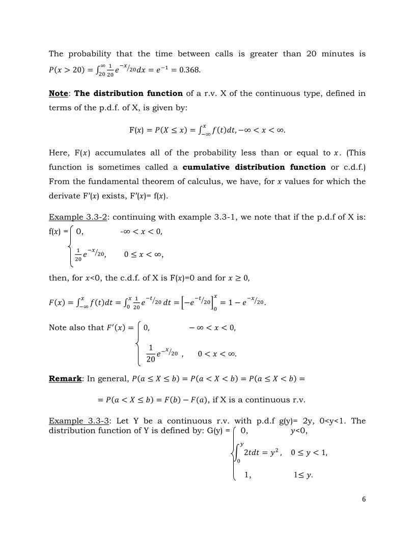
The probability that the time between calls is greater than 20 minutes is

Note: The distribution function of a r.v. X of the continuous type, defined in

terms of the p.d.f. of X, is given by:

F( )

Here, F( ) accumulates all of the probability less than or equal to . (This

function is sometimes called a cumulative distribution function or c.d.f.)

From the fundamental theorem of calculus, we have, for values for which the

derivate F’( ) exists, F’( )= f( ).

Example 3.3-2: continuing with example 3.3-1, we note that if the p.d.f of X is:

f( ) = 0, -

,

then, for <0, the c.d.f. of X is F( )=0 and for

.

Note also that

Remark: In general,

, if X is a continuous r.v.

Example 3.3-3: Let Y be a continuous r.v. with p.d.f g(y)= 2y, 0<y<1. The

distribution function of Y is defined by: G(y) = 0, <0,

1, 1

7

Also, P

and

Note: Let X be a continuous r.v. with a p.d.f f( ). Then the expected value of X,

or the mean of X, is

and the variance of X is:

The standard deviation of X is , and the moment-generating

function, if it exists, is:

M(t) =

Moreover, important results such as

are still valid.

Remark: In both the discrete and continuous cases, note that if the rth

moment, E(Xr), exists and is finite, then the same is true of all lower order

moments, E(Xk), k=1,2,…, r-1. However, the converse is not true; for example,

the first moment can exist and be finite, but the second moment is not

necessarily finite. Moreover, if exists and is finite for –h<t<h, then all

moments exist and are finite, but the converse is not necessarily true.

Example 3.3-4: For the r.v. Y in example 3.3.3

Note: The (100P)th percentile is a number such that the area under f(x) to

the left of is P. That is,

8

. The 50th percentile is called the median. We let

m= which is also called the second quartile. The 25th and 75th

percentiles are called the first and third quartiles, respectively, and are denoted

by

The (100p)th percentile of a distribution is often called the quantile of order P.

So if are the order statistics associated with the sample x1,

x2,….,xn, then yr is called the quantitle of order

th percentile. Also, the percentile of a theoretical

distribution is the quantile of order P. Now, suppose the theoretical distribution

is a good model for the observations. Then if we plot ,

for several values of r (possibly even for all r values, r= 1,2,…,n), we would

expect these points to lie close to a line through the origin with slope

equal to 1 because . If they are not close to that line, then we would

doubt that the theoretical distribution is a good model for the observations. The

plot of for several values of r is called the quantile-quantile plot or the

q-q plot.

Example 3.3-5: The time X in months until failure of a certain product has the

p.d.f. (of the Weibull type)

Its distribution function is

For example, the 30th percentile,

⇨ 1-

⇨ 1-

9

⇨

Likewise,

So

Thus, P(2.84<X<5.28)=0.6.

3.4. The uniform and Exponential Distributions

The r.v. X has a uniform distribution (or rectangular) if its pdf is equal to a

constant on its support. If the support is the interval [a,b], then

Moreover, we shall say that X is U(a,b). The distribution function of X is:

F( )= 0, x<a,

1 ,

Thus, when a< <b, we have f( )= F’( )= .

The mean, variance, and moment-generating function of X are, respectively,

1, t=0.

An important uniform distribution is that for a=0 and b=1, namely, U(0,1). If X

is U(0,1), approximate values of X can be simulated on most computers with

the use of a random-number generator.

Example: Let X have the p.d.f. f( ) = , 0< <100, so that X is U(0,100).

The mean and the variance are, respectively,

10

Definition: The r.v. X has an exponential distribution if its p.d.f. is defined by

Accordingly, the waiting time

W until the first change in a Poisson process has an exponential distribution

with .

Then the m.g.f of X is: M(t)=

=

Thus,

Hence, for an exponential distribution, we have

.

So if λ is the mean number of changes in the unit interval, then is the

mean waiting time for the first change.

Example: Let X have an exponential distribution with a mean of Then

the p.d.f. of X is given by: f( ) =

Let X have an exponential distribution with mean Then the distribution

function of X is F( ) = 0

The median, m, is found by solving F(m) = 0.5; that is,

11

So with

Remark: For an exponential r.v. X, we have

Example: customers arrive in a certain shop according to an approximate

Poisson process at a mean rate of 20 per hour. What is the probability that the

shopkeeper will have to wait more than 5 minutes for the arrival of the first

customer?

Solution: Let X denote the waiting time in minutes until the first customer

arrives, and note that λ , is the expected number of arrivals per minute.

Thus, =

and the median time until the first arrival is m=-3 ln(0.5)=2.0794.

Example: Suppose that a certain type of electronic component has an

exponential distribution with a mean life of 500 hours. If X denotes the life of

this component, then

If the component has been in operation for 300 hours, the conditional

probability that it will last for another 600 hours is:

which is exactly equal to

.

Hence, the exponential distribution is probably not the best model for the

probability distribution of such a life.

12

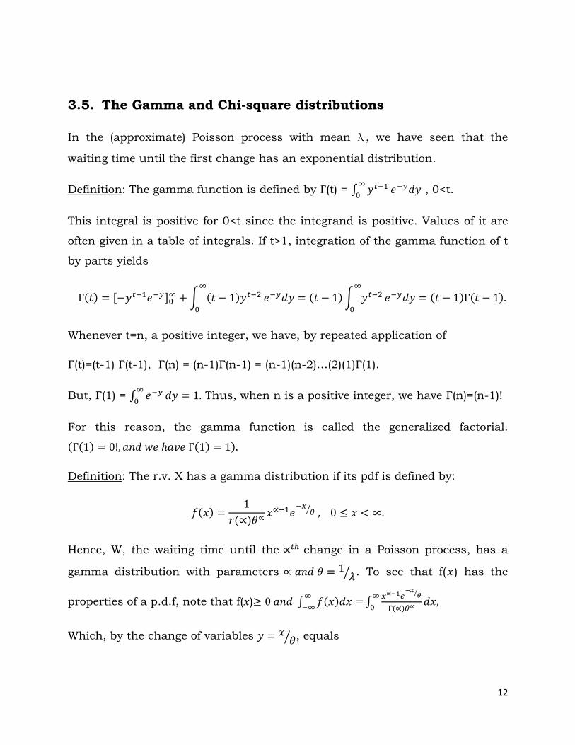
3.5. The Gamma and Chi-square distributions

In the (approximate) Poisson process with mean λ , we have seen that the

waiting time until the first change has an exponential distribution.

Definition: The gamma function is defined by (t) =

, 0<t.

This integral is positive for 0<t since the integrand is positive. Values of it are

often given in a table of integrals. If t>1, integration of the gamma function of t

by parts yields

Whenever t=n, a positive integer, we have, by repeated application of

Г(t)=(t-1) Г(t-1), Г(n) = (n-1)Г(n-1) = (n-1)(n-2)…(2)(1)Г(1).

But, Г(1) =

Thus, when n is a positive integer, we have Г(n)=(n-1)!

For this reason, the gamma function is called the generalized factorial.

Definition: The r.v. X has a gamma distribution if its pdf is defined by:

Hence, W, the waiting time until the change in a Poisson process, has a

gamma distribution with parameters . To see that f( ) has the

properties of a p.d.f, note that f( )

Which, by the change of variables , equals

13

The m.g.f. of X is M(t)

.

The mean and variance are:

Example 3.5-1: Suppose the number of customers per hour arriving at a shop

follows a Poisson process with mean 30. What is the probability that the shop

keeper will wait more than 5 minutes before both of the first two customers

arrive?

Solution: If a minute is our unit, then = If X denotes the waiting time in

minutes until the second customer arrives, then X has a gamma distribution

with . Hence,

Example 3.5-2: Telephone calls arrive at a switchboard at a mean rate of =2

per minute according to a Poisson process. Let X denote the waiting time in

minutes until the fifth call arrives. The p.d.f. of X, with

is

The mean and the variance of X are, respectively, .

Definition: Let X have a gamma distribution with , where r is a

positive integer. The p.d.f. of X is:

14

We say that X has a chi-square distribution with r degrees of freedom, which

we abbreviate by saying that X is x2 (r).

It is a special case of the gamma distribution that plays an important role in

statistics. The mean and the variance of this chi-square distribution are,

respectively,

i.e. the mean equals the number of degrees of freedom, and the variance equals

twice the number of degrees of freedom,

Its m.g.f. is M(t) =

.

Remark: For the chi-square distribution, the values of the distribution function

for selected values of r and x, are given in Table IV.

Example 3.5-3: Let X have a chi-square distribution with r=5 degrees of

freedom (d.f.). Then, using Table IV in the appendix, we obtain

Example: If X is x2(7), then two constants, a and b, such that P(a<X<b)=0.95,

are a=1.690 and b=16.01. Other constants, a and b can be found, and we are

restricted in our choices only by the limited table.

Note: Let be a positive probability (usually less than 0.5), and let X have a

chi-square distribution with r d.f. Then

th percentile (or upper 100 th percent point).

Then the 100 th percentile is the number

That is, the probability to the right of

15

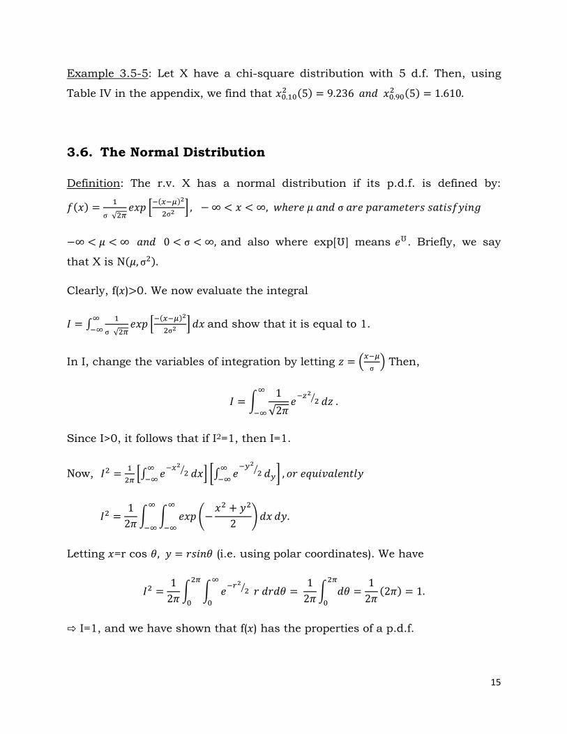
Example 3.5-5: Let X have a chi-square distribution with 5 d.f. Then, using

Table IV in the appendix, we find that

3.6. The Normal Distribution

Definition: The r.v. X has a normal distribution if its p.d.f. is defined by:

and also where exp[ ] means . Briefly, we say

that X is N

Clearly, f( ) 0. We now evaluate the integral

and show that it is equal to 1.

In I, change the variables of integration by letting

Then,

Since I>0, it follows that if I2=1, then I=1.

Now,

Letting =r cos (i.e. using polar coordinates). We have

I=1, and we have shown that f( ) has the properties of a p.d.f.

16

The m.g.f. of X is M(t)=

To evaluate this integral, we complete the square in the exponent:

Note that the integrand in the last integral is like the p.d.f. of a normal

distribution with which integrates to 1. Thus,

.

Now,

, and

Consequently, E(X)= M’(0)=

Var(X)= M’’(0)- .

That is, the parameters in the p.d.f. of X are the mean and the variance

of X.

Example 3.6-1: If the p.d.f. of X is

then X is N(-7,16). That is, X has a normal distribution with a mean

M(t)=exp

Example 3.6-2: If the m.g.f. of X is M(t)=exp

17

Note: If Z is N(0,1), we shall say that Z has a standard normal distribution.

Moreover, the distribution function of Z is:

Φ(Z)= P

Values of Φ (z) for are given in Table Va in the appendix. Because of the

symmetry of the standard normal p.d.f., it is true that Φ(-z)= 1- Φ(z) for all real

z. Moreover, when z>0, Φ(-z)=P(Z can be read directly from Table

Vb.

Example 3.6-3: If Z is N(0,1), then using Table Va in the appendix, we obtain

Now using Table Vb, we find that P(Z>1.24)=0.1075,

P , and using both tables, we obtain

P = 0.7794 - 0.0162=0.7632 .

Example 3.6-4: If the distribution of Z is N(0,1), then find the constants a and b

such that P(Z a)=0.9147 and = 0.0526 .

Solution: From Table Va, we see that a=1.37, and from Table V b, we see that

b= 1.62.

In statistical applications, we are often interested in finding a number

, where Z is N(0,1) and is usually less than 0.5.

Because of the symmetry of the normal p.d.f.,

Also, since the subscript of is the right-tail probability,

For example,

18

Example 3.6-5: To find Thus, z0.0125=2.24,

from Table Vb in the appendix. Also, z0.05=1.645 and z0.025=1.960, from the last

rows of Table Va.

Remark: If Z is N(0,1), then since P it follows that P

th percentile for the standard normal distribution,

N(0,1). For example, z0.05=1.645 is the 100(1-0.05)=95th percentile and

z0.95= -1.645 is the 100(1-0.95)= 5th percentile.

Theorem 3.6-1: If X is N

is N(0,1).

Proof: The distribution function of Z is:

Now, we use the change of variable of integration given by w= (i.e. =

wσ+ to obtain

But this is the expression for (z), a c.d.f. of a standardized normal random

variable. Hence, Z is N (O, 1).

Remark: If E(X)= µ and E = exists and Z = (X-µ)/ ,

Then = E(Z) = E[(X-µ)/ =

= 0, and

= E[(

)]= E[(

)]=

=1.

i.e If X is N(µ, ), then Z is N(0,1).

19

Theorem 3.6-1 can be used to find probabilities relating to X, as follows:

P(a )= P(

)=

) - (

).

Example 3.6-6: If X is N(3,16), then

P( 4 ) = P(

) = (1.25) - (0.25)= 0.8944-0.5987=

0.2957, and P(-2

Example 3.6-7: If X is N(25,36), find a constant c such that P(

Solution: We want P(-C/6

Thus, (

) – [1- (

)] = 0.9544 and ( c/6) =0.9772.

Hence, c/6=2 and c=12.

Theorem 3.6-2: If the r.v. X is N( ),

=( / = is (1).

Example 3.6-8 : If Z is N(0,1), then P( ) =0.95,

and P( from the chi-square table with r=1.