177
Lectures on Topics In Finite Element Solution of Elliptic Problems By Bertrand Mercier Tata Institute of Fundamental Research Bombay 1979
| Date post: | 05-May-2018 |
| Category: |
Documents |
| Upload: | nguyendieu |
| View: | 215 times |
| Download: | 2 times |

Lectures onTopics In Finite Element Solution of
Elliptic Problems
By
Bertrand Mercier
Tata Institute of Fundamental ResearchBombay
1979
Lectures onTopics In Finite Element Solution of
Elliptic Problems
By
Bertrand Mercier
Notes By
G. Vijayasundaram
Published for the
Tata Institute of Fundamental Research, Bombay
Springer-VerlagBerlin Heidelberg New York
1979
AuthorBertrand MercierEcole Polytechnique
Centre de Mathematiques Appliquees91128 Palaiseau (France)
c© Tata Institute of Fundamental Research, 1979
ISBN 3–540–09543–8 Springer-Verlag Berlin. Heidelberg. New YorkISBN 0–387–09543–8 Springer-Verlag New York Heidelberg. Berlin
No part of this book may be reproduced in anyform by print, microfilm or any other means with-out written permission from the Tata Institute ofFundamental Research, Bombay 400 005
Printed by N.S. Ray at The Book Centre Limited,Sion East, Bombay 400 022 and published by H. Goetze
Springer-Verlag, Heidelberg, West Germany
Printed In India

iv

Preface
THESE NOTES SUMMARISE a course on the finite element solutionof Elliptic problems, which took place in August 1978, in Bangalore.
I would like to thank Professor Ramanathan without whom thiscourse would not have been possible, and Dr. K. Balagangadharan whowelcomed me in Bangalore.
Mr. Vijayasundaram wrote these notes and gave them a much betterform that what I would have been able to.
Finally, I am grateful to all the people I met in Bangalore since theyhelped me to discover the smile of India and the depth of Indian civi-lization.
Bertrand MercierParis, June 7, 1979.
v

vi Preface
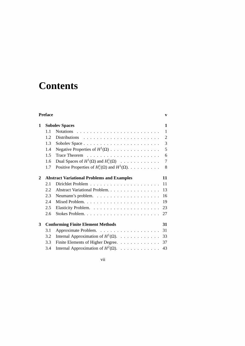
Contents
Preface v
1 Sobolev Spaces 11.1 Notations . . . . . . . . . . . . . . . . . . . . . . . . . 11.2 Distributions . . . . . . . . . . . . . . . . . . . . . . . 21.3 Sobolev Space . . . . . . . . . . . . . . . . . . . . . . . 31.4 Negative Properties ofH1(Ω) . . . . . . . . . . . . . . . 51.5 Trace Theorem . . . . . . . . . . . . . . . . . . . . . . 61.6 Dual Spaces ofH1(Ω) andH1
(Ω) . . . . . . . . . . . . 71.7 Positive Properties ofH1
(Ω) andH1(Ω). . . . . . . . . . 8
2 Abstract Variational Problems and Examples 112.1 Dirichlet Problem . . . . . . . . . . . . . . . . . . . . . 112.2 Abstract Variational Problem. . . . . . . . . . . . . . . . 132.3 Neumann’s problem. . . . . . . . . . . . . . . . . . . . 162.4 Mixed Problem. . . . . . . . . . . . . . . . . . . . . . . 192.5 Elasticity Problem. . . . . . . . . . . . . . . . . . . . . 232.6 Stokes Problem. . . . . . . . . . . . . . . . . . . . . . . 27
3 Conforming Finite Element Methods 313.1 Approximate Problem. . . . . . . . . . . . . . . . . . . 313.2 Internal Approximation ofH1(Ω). . . . . . . . . . . . . 333.3 Finite Elements of Higher Degree. . . . . . . . . . . . . 373.4 Internal Approximation ofH2(Ω). . . . . . . . . . . . . 43
vii

viii CONTENTS
4 Computation of the Solution of the Approximate Problem 494.1 Introduction . . . . . . . . . . . . . . . . . . . . . . . . 494.2 Steepest Descent Method . . . . . . . . . . . . . . . . . 504.3 Conjugate Gradient method . . . . . . . . . . . . . . . . 524.4 Computer Representation of a Triangulation . . . . . . . 554.5 Computation of the Gradient. . . . . . . . . . . . . . . . 564.6 Solution by Direct Methods . . . . . . . . . . . . . . . . 58
5 Review of the Error Estimates for the... 65
6 Problems with an Incompressibility Constraint 716.1 Introduction . . . . . . . . . . . . . . . . . . . . . . . . 716.2 Approximation Via Finite Elements of Degree 1 . . . . . 726.3 The Fraeijs De Veubeke - Sander Element . . . . . . . . 756.4 Approximation of the Stokes Problem... . . . . . . . . . 776.5 Penalty Methods. . . . . . . . . . . . . . . . . . . . . . 786.6 The Navier-Stokes Equations. . . . . . . . . . . . . . . 786.7 Existence and Uniqueness of Solutions of... . . . . . . . 796.8 Error Estimates for Conforming Method . . . . . . . . . 82
7 Mixed Finite Element Methods 857.1 The Abstract Continuous Problem . . . . . . . . . . . . 857.2 The Approximate Problem . . . . . . . . . . . . . . . . 917.3 Application to the Stokes Problem . . . . . . . . . . . . 937.4 Dual Error Estimates foru− uh . . . . . . . . . . . . . . 967.5 Nonconforming Finite Element Method for... . . . . . . 987.6 Approximate Brezzi Condition . . . . . . . . . . . . . . 1047.7 Dual Error Estimate for the Multiplier . . . . . . . . . . 1077.8 Application to Biharmonic Problem . . . . . . . . . . . 1087.9 General Numerical Methods for the... . . . . . . . . . . 1107.10 Equilibrium Elements for the Dirichlet Problem . . . . . 1137.11 Equilibrium Elements for the Plate Problem . . . . . . . 118
8 Spectral Approximation for Conforming Finite... 1298.1 The Eigen Value Problem . . . . . . . . . . . . . . . . . 1298.2 The Operator⊤ . . . . . . . . . . . . . . . . . . . . . . 130

CONTENTS ix
8.3 Example . . . . . . . . . . . . . . . . . . . . . . . . . . 1308.4 Approximate Problem . . . . . . . . . . . . . . . . . . . 1318.5 Convergence and Error Estimate for the Eigen Space. . . 1328.6 Error Estimates for the Eigen Values. . . . . . . . . . . . 1348.7 Improvement of the Error Estimate for the... . . . . . . . 136
9 Nonlinear Problems 1419.2 Generalization . . . . . . . . . . . . . . . . . . . . . . . 1469.3 Contractive Operators. . . . . . . . . . . . . . . . . . . 1479.4 Application to Unconstrained Problem . . . . . . . . . . 1549.5 Application to Problems with Constraint. . . . . . . . . 156
Bibliography 163

x CONTENTS

Chapter 1
Sobolev Spaces
IN THIS CHAPTER the notion of Sobolev spaceH1(Ω) is introduced. 1
We state the Sobolev imbedding theorem, Rellich theorem, and Tracetheorem forH1(Ω), without proof. For the proof of the theorems thereader is referred to ADAMS [1].
1.1 Notations
LetΩ ⊂ Rn(n = 1, 2 or 3) be an open set. LetΓ denote the boundary ofΩ, it is assumed to be bounded and smooth. Let
L2(Ω) =
f :∫
Ω
| f |2 dx< ∞
and
( f , g) =∫
Ω
f g dx
ThenL2(Ω) is a Hilbert space with (· , · ) as the scalar product.
1

2 1. Sobolev Spaces
1.2 Distributions
Let D(Ω) denote the space of infinitely differentiable functions withcompact support inΩ. D(Ω) is a nonempty set. If
f (x) =
exp(
1|x|2−1
)
if |x| < 1
0 if |x| ≥ 1
then f (x)ǫD(Ω),Ω = R.The topology chosen forD(Ω) is such that a sequence of elements
φn in D(Ω) converges to an elementφ belonging toD(Ω) in D(Ω) ifthere exists a compact setK such that
supp φn, supp φ ⊂ K
Dαφn → Dαφ uniformly for each multi-indexα = (α1, . . . , αn) where2
Dαφ stands for∂α1+...+αnφ
∂α1 x1 · · · ∂αn xn.
A continuous linear functional onD(Ω) is said to be adistribution.The space of distributions is denoted byD ′(Ω). We use<· , ·> for theduality bracket betweenD ′(Ω) andD(Ω).
EXAMPLE 1. (a) A square integrable function defines a distribu-tion: If f ǫL2(Ω) then
〈 f , φ〉 =∫
Ω
fφdx for all φǫD(Ω)
can be seen to be a distribution. We identifyL2(Ω) as a space ofdistribution, i.e.
L2(Ω) ⊂ D′(Ω).
(b) The dirac massδ, concentrated at the origin, defined by
〈δ, φ〉 = φ(0) for all φǫD(Ω)
defines a distribution.
1.3. Sobolev Space 3
DEFINITION. Derivation of a DistributionIf f is a smooth function andφǫD(Ω) then using integration by parts
we obtain∫
Ω
∂ f∂xi
φdx= −∫
Ω
f∂φ
∂xidx.
This gives a motivation for defining the derivative of a distribution. 3
If TǫD ′(Ω) andα is a multi index then DαTǫD ′(Ω) is defined by
〈DαT, φ〉 = (−1)|α|〈T,Dαφ〉 ∀φǫD(Ω).
If Tn,TǫD ′(Ω) then we say Tn→ T in D ′(Ω) if
〈Tn, φ〉 → 〈T, φ〉 for all φǫD(Ω).
The derivative mapping Dα : D ′ → D ′ is continuous since if Tn →T in D ′ then
〈DαTn, φ〉 = (−1)|α|〈Tn,Dαφ〉
→ (−1)|α|〈T,Dαφ〉= 〈DαT, φ〉 for all φǫD(Ω).
1.3 Sobolev Space
The Sobolev spaceH1(Ω) is defined by
H1(Ω) =
vǫL2(Ω) :∂v∂xi
ǫL2(Ω), 1 ≤ i ≤ n
where the derivatives are taken in the sense of distribution.
f ǫL2(Ω) need not imply∂ f∂xi
ǫL2(Ω).
EXAMPLE 2. LetΩ = [−l, l]
f (x) =
−1 if x < 0
0 if x ≥ 0.
Then f ǫL2[−l, l]; but d f/dx = δ is not given by a locally integrablefunction and hence not by anL2 function.
4 1. Sobolev Spaces
We define an inner product (· , · )1 in H1(Ω) as follows: 4
(u, v)1 = (u, v) +n
∑
i=1
(
∂u∂xi
,∂v∂xi
)
for all u, vǫH1(Ω).
Let ‖· ‖1 be the norm associated with this inner product. Then
LEMMA 1. H1(Ω) with ‖· ‖1 is a Hilbert spaces.
Proof. Let u j be a Cauchy sequence inH1(Ω). This imply
u j,
∂u j
∂xi
i = 1, 2, . . . , n
are Cauchy inL2. Hence there existsv, viǫL2(Ω)1 ≤ i ≤ n such that
u j → v in L2(Ω),
∂u j
∂xi→ vi in L2(Ω), 1 ≤ i ≤ n,
For anyφǫD(Ω),⟨
∂u j
∂xi, φ
⟩
= −⟨
u j ,∂φ
∂xi
⟩
→ −⟨
u,∂φ
∂xi
⟩
=
⟨
∂u∂xi
, φ
⟩
.
But⟨
<∂u j
∂xi, φ
⟩
→ 〈vi , φ〉 .
Hence
vi =∂u∂xi
.
Thus
u j → u in L2(Ω)
∂u j
∂xi→
∂u∂xi
in L2(Ω).
This provesu j → u in H1(Ω). 5

1.4. Negative Properties ofH1(Ω) 5
1.4 Negative Properties ofH1(Ω)
(a) The functions inH1(Ω) need not be continuous except in the casen = 1.
EXAMPLE 3. Let
Ω =
(x, y)ǫR2 : x2+ y2 < r2
, r < 1.
f (r) = (log 1/r)k, k < 1/2 where
r = (x2+ y2)1/2.
Then f ǫH1(Ω) but f is not continuous at the origin.
In the casen = 1, if uǫH1(Ω),Ω ⊂ R1 thenu can be shown to becontinuous using the formula
u(y) − u(x) =
y∫
x
dudx
(s) ds
wheredu/dsdenotes the distributional derivative ofu.
(b) D(Ω) is not dense inH1(Ω). To see this letuǫ(D(Ω))⊥ in H1 andφǫD(Ω). We have
(u, φ)1 = (u, φ) +n
∑
i=1
(
∂u∂xi
,∂φ
∂xi
)
= 0
i.e. 〈u, φ〉 +n
∑
i=1
⟨
−∂2u
∂x2i
, φ
⟩
= 0
Thus
〈−∆u+ u, φ〉 = 0 for all φǫD(Ω).
Hence
−∆u+ u = 0 in D′(Ω).
6 1. Sobolev Spaces
LetΩ = xǫRn : |x| < 1, 6
u(x) = er.x where rǫRn,
∆u(x) = |r |2er.x= |r |2u.
= u if |r | = 1.
Thus whenn = 1, u with r = ±1 belongs toD(Ω))⊥, whenn > 1there are infinitely manyr′s(rǫSn−1) such thatuǫ(D(Ω))⊥. Moreoverthese functions for differentr ’s are linearly independent. Therefore
dimension (D(Ω))⊥ ≥ 2 if n = 1
dimension (D(Ω))⊥ = ∞ if n > 1.
This proves the claim (b).We shall defineH1
(Ω) as the closure ofD(Ω) in H1(Ω). We havethe following inclusions
D(Ω) ⊂dense
H1(Ω) ⊂ H1(Ω) ⊂
denseL2(Ω).
1.5 Trace Theorem
Let Ω be a bounded open subset ofRn with a Lipschitz continuousboundaryΓ : i.e. there exists finite number of local chartsa j , 1 ≤ j ≤ Jfrom y′ǫRn−1 : |y′| < α into Rn and a numberβ > 0 such that
Γ =
J⋃
j=1
(y′, yn) : yn = a j(y′), |y′| < α
,
(y′, yn) : a j(y′) < yn < a j(y
′) + β, |y′| < α
⊂ Ω, 1 ≤ j ≤ J,
(y′, yn) : a j(y′) − β < yn < a j(y
′), |y′| < α
⊂ CΩ, 1 ≤ j ≤ J.
It can be proved thatC∞(Ω) is dense inH1(Ω). If f ǫC∞(Ω) we7
define the trace off , namelyγ f , by
γ f = f |Γ. Note γ f ǫL2(Γ) if f ǫC∞(Ω)
1.6. Dual Spaces ofH1(Ω) andH1(Ω) 7
γ : C∞(Ω)→ L2(Γ) is continuous and linear with norm‖ γu ‖L2(Γ)≤C ‖ u ‖1. Hence this can be extended as continuous linear map fromH1(Ω) to L2(Γ).
H1(Ω) is characterised by
THEOREM 2.H1(Ω) = vǫH1(Ω) : γV = 0
1.6 Dual Spaces ofH1(Ω) and H1(Ω)
The mapping
I : H1(Ω)→ (L2(Ω))n+1 defined by
I (v) =
(
v,∂v∂x1
, . . . ,∂v∂xn
)
is easily seen to be an isometric isomorphism ofH1(Ω)) into subspaceof (L2(Ω))n+1. If f ǫ(H1(Ω))′ thenF : I (H1(Ω))→ R with F(Iu) = f (u)is a continuous linear functional onI (H1(Ω)). Hence by Hahn Ba-nach theoremF can be extended to (L2(Ω))n+1. Therefore, there exists(v, v1, . . . , vn)ǫ(L2(Ω))n+1 such that
f (u) = F(Iu) = (v, u) +n
∑
i=1
(vi , ∂u/∂xi).
This representation is not unique sinceF cannot be extended uniquelyto (L2(Ω))n+1 For allφǫD(Ω) we have
f (φ) = 〈v, u〉 −n
∑
i=1
⟨
∂vi
∂xi, φ
⟩
,
Thus 8
f |D(Ω) = v−n
∑
i=1
∂vi
∂xi.
Conversely ifTǫD ′(Ω) is given by
T = v−n
∑
i=1
∂vi
∂xi,
8 1. Sobolev Spaces
wherev, viǫL2(Ω), 1 ≤ i ≤ n thenT can be extended as a continuouslinear functional onH1(Ω) by the prescription
T(u) = (v, u) +n
∑
i=1
(
vi ,∂u∂xi
)
for all uǫH1(Ω).
The extension ofT to H1(Ω) need not be unique. But we will provethat the extension ofT to H1
(Ω) is unique. LetTǫ(H1 (Ω))′ be such that
T |D(Ω) = T.Let uǫH1
(Ω). Then there existsumǫD(Ω) such thatum → u in H1.Now
T(u) = T( limin H1
um) = limm
T(um)
= limm
T(um)
= limm
(v, um) +n
∑
i=1
(
vi ,∂um
∂xi
)
= (v, u) +n
∑
i=1
(
vi ,∂u∂xi
)
ThusT = T on H1
(Ω).
Hence we identify (H1(Ω))′ with a space of distribution and we de-9
note it byH−1(Ω). That is
H−1(Ω) =
v−n
∑
i=1
∂vi
∂xi: (v, v1, . . . , vn)ǫ(L2(Ω))n+1
⊂ D′(Ω).
EXERCISE 1. Show that∂/∂xi : L2(Ω)→ H−1(Ω) is continuous.
1.7 Positive Properties ofH1(Ω) and H1(Ω).
THEOREM 3. (Poincare’s Inequality). LetΩ be an open boundedsubset ofRn. Then there exists a constant C(Ω) such that
∫
Ω
v2 dx≤ C(Ω)∫
Ω
|∇v|2 dx for all vǫH1 (Ω).

1.7. Positive Properties ofH1(Ω) andH1(Ω). 9
Proof. We shall prove the inequality for the functions inD(Ω) and usethe density ofD(Ω) in H1
(Ω).SinceΩ is bounded, we have
Ω ⊂ [a1, b1] × . . . × [an, bn].
For anyu(x)ǫD(Ω), we have
u(x) =
xi∫
ai
∂u∂xi
(x1, . . . , xi−1, t, xi+1, . . . , xn) dt.
Thus
|u(x)| ≤ (bi − ai)1/2
bi∫
ai
∣
∣
∣
∣
∣
∂u∂xi
∣
∣
∣
∣
∣
2
dt
1/2
Squaring both sides and integrating we obtain
b1∫
a1
· · ·bn
∫
an
|u(x)|2 dx≤ (bi − ai)2
b1∫
a1
· · ·bn
∫
an
∣
∣
∣
∣
∣
∂u∂xi
∣
∣
∣
∣
∣
2
dx.
Thus 10∫
Ω
|u(x)|2 dx≤ C(Ω)∫
Ω
|∇u|2 dx
whereC(Ω) = (b1 − a1)2
+ · · · + (bn − an)2.
Let vǫH1 (Ω). Then there existsunǫD(Ω) such thatun → v in H1,
which impliesun → v in L2 and∂un
∂xi→
∂v∂xi
in L2. Using this and the
inequality for smooth functions we arrive at the result.
REMARK 1. The theorem is not true for functions in H1(Ω). For ex-ample a nonzero constant function belongs to H1(Ω) but does not satisfythe above inequality.
We state Sobolev imbedding theorem and Rellich’s theorem, whichhave many important applications.

10 1. Sobolev Spaces
SOBOLEV IMBEDDING THEOREM 4. If Ω is an open bounded sethaving a Lipschitz continuous boundary then we have the imbedding
H1(Ω) → Lp(Ω),
p < q or p≤ q according as n= 2 or n > 2 where
1/q = 1/2− 1/n.
RELLICH’S THEOREM 5. The above imbedding is compact forp < q.
Chapter 2
Abstract VariationalProblems and Examples
IN SECTION 1 OF this chapter, we give a variational formulation of the 11
Dirichlet problem. In section 2 we prove the existence and uniquenessresults for the abstract variational problem. In the remaining sections,we deal with the Neumann problem, Elasticity problem, Stokes problemand Mixed problem and their variational formulations.
2.1 Dirichlet Problem
The Dirichlet problem is to findu such that
−∆u = f in Ω (2.1)
u = 0 on Γ (2.2)
whereΩ ⊂ Rn is a bounded open set with smooth boundaryΓ and f is agiven function.
Multiplying equation (2.1) by a smooth functionv which vanishesonΓ and integrating, we obtain
∫
Ω
−∆u.v dx=∫
Ω
f .v dx (2.3)
11
12 2. Abstract Variational Problems and Examples
Formally, using integration by parts and the fact thatv = 0 onΓ, wesee that
∫
Ω
∇v.∇u dx=∫
Γ
∂u∂n
v dΓ −∫
Ω
∆u v dx=∫
Ω
−∆u.v dx (2.4)
Equations (2.3) and (2.4) give∫
Ω
∇u.v dx=∫
Ω
f v dx.
Now, setting
a(u, v) =∫
Ω
∇u.∇v dx
and12
L(v) =∫
Ω
f v dx,
problem (2.1) can be formulated thus:Find uεV such that
a(u, v) = L(v) for all vεV, (2.5)
whereV has to be chosen suitably.Sincea(· , · ) is symmetric, (2.5) is Euler’s condition for the mini-
mization problemJ(u) = inf
vεVJ(v), (2.6)
whereJ(v) = 1/2a(v, v) − L(v).
If u is the solution of the minimization problem then it can be shownthat
(J′(u), v) = 0 for all vεV, (2.7)
where (J′(u), v) is the Gateaux derivative ofJ in the directionv.When a(· , · ) is symmetric one can show that problems (2.5) and
(2.6) are equivalent.
2.2. Abstract Variational Problem. 13
To haveJ(v) finite, we want our spaceV to be such that∇v εL2(Ω),fεL2(Ω) for all vεV. The largest space satisfying the above conditionsand (2.2) isH1
(Ω) and hence we chooseV to beH1(Ω).
If u is a solution of (2.5) then∫
Ω
∇u.∇v dx=∫
Ω
f v dx for all vεD(Ω) ⊂ H1(Ω).
This implies that 13
〈−∆u, v〉 = 〈 f , v〉 for all vεD(Ω);
so− ∆u = f in D
′. (2.8)
Conversely, ifuεH1(Ω) satisfies (2.8), retracing the above steps we
obtaina(u, v) = f (v) for all vεD(Ω). (2.9)
SinceD(Ω) is dense inH1(Ω), (2.9) holds for allvεV = H1
(Ω). Thusuis the solution of (2.5).
2.2 Abstract Variational Problem.
We now prove the existence and uniqueness theorem for the abstractvariational problem.
THEOREM 1. Let V be a Hilbert space and a(· , · ) : V × V → R becontinuous and bilinear. Further, assume that a(· , · ) is coercive: thereexistsα > 0 such that a(v, v) ≥ α ‖ v ‖2V for all vεV. Let L be acontinuous linear functional on V. Then the problem:
To find uεV such that
a(u, v) = L(v), for all vεV (2.10)
has a unique solution.
14 2. Abstract Variational Problems and Examples
Proof. (i) Uniqueness. Let u1, u2εV be two solutions of (2.10).Therefore
a(u1, v) = L(v),
a(u2, v) = L(v), for all vεV.
Subtracting one from the other, takingv = u2 − u1 and usingV-14
coercivity ofa(· , · ), we obtain
α ‖ u1 − u2 ‖2V≤ a(u1 − u2, u1 − u2) = 0,
Thusu1 = u2.
(ii) Existence whena(· , · ) is symmetric. Sincea(· , · ) is symmetric,the bilinear forma(u, v) is a scalar product onV and the associatednorma(v, v)1/2 is equivalent to the norm inV. Hence, by the Rieszrepresentation theorem there existsσLεV such that
a(σL, v) = L(v) for all vεV.
Hence the theorem is true in the symmetric case.
(iii) Existence in the general case.Let wεV. The functionLw : V →R defined by
Lw(v) = (w, v) − ρ(a(w, v) − L(v))
is linear and continuous. Hence by the Riesz representationtheo-rem there exists auεV such that
Lw(v) = (u, v).
Let T : V → V be defined by
Tw= u
whereu is the solution of the equation
Lw(v) = (u, v) for all vεV.
2.2. Abstract Variational Problem. 15
we will show thatT is a contraction mapping. HenceT has a unique15
fixed point which will be the solution of (2.10).Let
u1 = Tw1, u2 = Tw2.
Thus
(u1 − u2, v) = (w1 − w2, v) − ρa(w1 − w2, v) ∀vεV (2.11)
Let A : V → V, whereAu is the unique solution of
(Au, v) = a(u, v) for all vεV,
which exists by the Riesz representation theorem.
‖ Au ‖= supvεV
|(Au, v)|‖ v ‖
= supvεV
|a(u, v)|‖ v ‖
≤ M ‖ u ‖,
where|a(u, v)| ≤ M ‖ u ‖‖ v ‖. SoA is continuous. Equation (2.11) canbe written as
(u1 − u2, v) = (w1 − w2.v) − ρ(A(w1 − w2)v) for all vεV,
which implies that
u1 − u2 = (w1 − w2) − ρA(w1 − w2).
So
‖ u1 − u2 ‖2 =‖ w1 − w2 ‖2 −2ρ(A(w1 − w2),w1 − w2)
+ ρ2 ‖ A(w1 − w2) ‖2
≤‖ w1 − w2 ‖2 −2ρa(w1 − w2,w1 − w2)
+ ρ2M2 ‖ w1 − w2 ‖2, (using the continuity ofA)
≤‖ w1 − w2 ‖2 −2ρα ‖ w1 − w2 ‖2 +ρ2M2 ‖ w1 − w2 ‖2,
since 16
a(w1 − w2,w1 − w2) ≥ α ‖ w1 − w2 ‖2 .
16 2. Abstract Variational Problems and Examples
So‖ u1 − u2 ‖2≤ (1− 2ρα + ρ2M2) ‖ w1 − w2 ‖2 .
That is,
‖ Tw1 − Tw2 ‖≤√
(1− 2ρα + ρ2M2) ‖ w1 − w2 ‖ .
Choosingρ in ]0, α/2M[, we obtain thatT is a contraction.
This proves the theorem.
REMARK 1. This theorem also gives an algorithm to find the solutionof equation(2.10). Let uεV be given. Let un+1
= Tun. Then un → w,which is the fixed point of T, and also the solution of(2.10).
2.3 Neumann’s problem.
Neumann’s problem is to find anu such that
−∆u+ cu= f in Ω, (2.12)
∂u∂n= g on Γ. (2.13)
We now do the calculations formally to find out the bilinear form a (·, ·),the linear functionalL(·) and the spaceV.
For smoothv, (2.12) implies∫
Ω
(−∆u+ cu)v dx=∫
Ω
f v dx. (2.14)
From Green’s formula,17∫
Ω
∇u.∇v dx=∫
Γ
∂u∂n
v dΓ −∫
Ω
v∆u dx,
and by (2.14) we obtain∫
Ω
(∇u.∇v+ cuv) dx =∫
Ω
f v dx+∫
Γ
∂u∂n
v dΓ =∫
Ω
f v dx+∫
Γ
gv dΓ,
2.3. Neumann’s problem. 17
since∂u∂n= g onΓ, by (2.13). This suggests the definitions:
a(u, v) =∫
Ω
(∇u.∇v+ cuv) dx (2.15)
L(v) =∫
Ω
f v dx+∫
Γ
gv dΓ, (2.16)
V = H1(Ω), (2.17)
where fεL2(Ω) andgεL2(Γ).Clearlya(u, v) is bilinear, continuous and symmetric.
a(v, v) =∫
Ω
(
(∇v)2+ cv2
)
dx
≥ min1, c ‖ v ‖21,
which showsa(·, ·) is H1(Ω)-coercive.L(·) is a continuous linear functional onH1(Ω). Hence by the theo-
rem there exists a uniqueuεV = H1(Ω) such that∫
Ω
(∇u.∇v+ cuv) dx=∫
Ω
f v dx+∫
Γ
for all vεH1(Ω) (2.18)
From (2.18) we obtain that for allvεD(Ω), 18
〈−∆u+ cu, v〉 = 〈 f , v〉.
Hence
−∆u+ cu= f in D′(Ω) (2.19)
To find the boundary condition we use Green’s formula:∫
Ω
∇u.∇v dx=∫
Ω
−∆u.v dx+∫
Γ
∂u∂n
v dΓ,

18 2. Abstract Variational Problems and Examples
which holds for alluεH2(Ω) and for allvεH1(Ω).Assuming that our solutionuεH2(Ω), from (2.19) we have
∫
Ω
(−∆u+ cu)v =∫
Ω
f v for all vεH1(Ω).
Using Green’s formula we obtain∫
Ω
(∇u∇v+ cuv) dx =∫
Γ
∂u∂n
v dx+∫
Ω
f v dx.
This, together with (2.18), implies∫
Γ
(
g− ∂u∂n
)
v dΓ = 0 for all vεH1(Ω).
Hence we get the desired boundary condition
∂u∂n= g on Γ.
If uεH2(Ω), these are still valid in “some sense” which is given inLIONS–MAGENES [29].
REMARK 2. Even when g= 0 we cannot take the space
V1 =
vεH1(Ω) :∂v∂n= 0 on Γ
to be the basic space V, since V1 is not closed. In the Neumann problem19
2.3, we obtain the boundary condition from Green’s formula.In the caseof Dirichlet problem 2.1, we impose the boundary condition in the spaceitself.
REGULARITY THEOREM (FOR DIRICHLET PROBLEM) 2. IfΓ is C2 or Ω is a convex polygon and fεL2(Ω), then the solution u of theDirichlet problem(2.1), (2.2)belongs to H2(Ω).
REGULARITY THEOREM (FOR THE NEUMANN PROBLEM)3. If Γ is C2 or Ω is a convex polygon, fεL2(Ω) and g belongs to aspace finer than L2(Ω) (for example gεH1(Γ)), then the solution u of theNeumann problem(2.12), (2.13)belongs to H2(Ω).
For a proof of these theorems the reader is referred to NECAS [33].

2.4. Mixed Problem. 19
2.4 Mixed Problem.
In Sections 2.1 and 2.3 we found the variational formulationfrom thepartial differential equation. In the general case it is difficult to formulatethe variational problem from the p.d.e. In fact a general p.d.e. neednot give rise to a variational problem. So in this section, wewill takea general variational problem and find out the p.d.e. satisfied by itssolution.
Let Ω be a bounded open set with boundaryΓ. Let Γ = Γ ∪ Γ1 20
whereΓ andΓ1 are disjoint. Let
V =
vεH1(Ω) : v = 0 on Γ
. (2.20)
It is easy to see thatV is closed and hence a Hilbert space with‖· ‖1norm
Figure 2.1:
We will use summation convention here afterwards. Let
a(u, v) =∫
Ω
(
ai j (x)∂u∂xi
∂v∂x j+ a uv
)
dx, (2.21)
L(v) =∫
Ω
f v dx+∫
Γ
gv dΓ, (2.22)

20 2. Abstract Variational Problems and Examples
wherea > 0, ai j are smooth and there exists two constantsα andα1
such that
α1ξiξi ≥ ai j (x)ξiξ j ≥ αξiξi for allxεΩ, ξεRn (2.23)
i.e. the quadratic formai j (x)ξiξ j is uniformly continuous and uniformlypositive definite.
Inequality (2.23) implies that the bilinear forma(· , · ) is continuousandV-coercive. Formally we have
a(u, v) =∫
Ω
[
−∂
∂x j
(
ai j∂u∂xi
)
v+ auv
]
dx+∫
Γ
ai j∂u∂xi
n jv dΓ (2.24)
Let21∂u∂vA= ai j
∂u∂xi
n j ,
and
Au= −∂
∂x j
(
ai j∂u∂xi
)
.
If vεD(Ω) then the equation
a(u, v) = L(v) (2.25)
becomes〈Au, v〉 = 〈 f , v〉.
ThereforeAu= f in D
′(Ω). (2.26)
Now for all vεV, we have
a(u, v) =∫
Ω
Au.v+∫
Γ
∂u∂vA
v dΓ
=
∫
Ω
Au.v+∫
Γ1
∂u∂vA
v dΓ
L(v) =∫
Ω
f v dx+∫
Γ1
gv dΓ.

2.4. Mixed Problem. 21
Equations (2.25) and (2.26) imply, for allvεV,∫
Γ1
∂u∂vA
v dΓ =∫
Γ1
g v dΓ.
From this we obtain formally
∂u∂vA= g on Γ1. (2.27)
Thus the boundary value problem corresponding to the variational 22
problema(u, v) = L(v) for all vεV,
with a(· , · ), L(· ) andV given by the equations (2.20) - (2.22) is
Au= f in Ω,
∂u∂vA= g on Γ1,
u = 0 on Γ.
(2.28)
REMARK 3. Even when f and g are smooth the solution u of the prob-lem (2.28)may not be in H2(Ω). In general, we will have a singularityat the transition points A, B onΓ. But if Γ andΓ1 make a corner thenthe solution u may be in H2(Ω) provided that the boundary functionsf , g satisfy some compatibility conditions. For regularity theorems thereader is referred to an article by PIERRE GIRSVARD [22].
EXERCISE 1. Transmission Problem. Let Ω,Ω1,Ω2 be open setssuch thatΩ = Ω1 ∪ Ω2 ∪ S whereΩ1 andΩ2 are disjoint subsets ofΩ andS is the interface between them. Let
a(u, v) =2
∑
i=1
∫
Ωi
ai∇u.∇v dx,
L(v) =∫
Ω
f v dx,
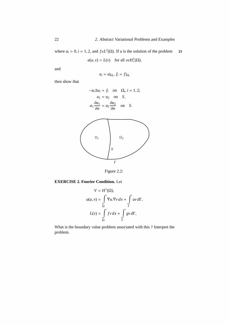
22 2. Abstract Variational Problems and Examples
whereai > 0, i = 1, 2, and fεL2(Ω). If u is the solution of the problem 23
a(u, v) = L(v) for all vεH1(Ω),
andui = u|Ωi , fi = f |Ωi
then show that
−ai∆ui = fi on Ωi , i = 1, 2;
u1 = u2 on S,
a1∂u1
∂n= a2
∂u2
∂non S.
Figure 2.2:
EXERCISE 2. Fourier Condition. Let
V = H1(Ω),
a(u, v) =∫
Ω
∇u.∇v dx+∫
Γ
uv dΓ,
L(v) =∫
Ω
f v dx+∫
Γ
gv dΓ,
What is the boundary value problem associated with this ? Interpret theproblem.

2.5. Elasticity Problem. 23
2.5 Elasticity Problem.
(a) 3-DIMENSIONAL CASE. LetΩ ⊂ R3 be a bounded, connected24
open set. LetΓ be the boundary ofΩ and letΓ be split into twopartsΓ andΓ1. LetΩ be occupied by an elastic medium, whichwe assume to be continuous. Let the elastic material be fixedalongΓ. Let (fi) be the body force acting inΩ and (gi ) be thepressure load acting alongΓ1. Let (ui (x)) denote the displacementat x.
Figure 2.3:
In linear elasticity the stress-strain relation is
σi j.(u) = λ(div u)δi j + 2µεi j (u), εi j (u) =12
(
∂ui
∂x j+∂u j
∂xi
)
, (2.29)
whereσi j andεi j denote the components of the stress and straintensors respectively.
The problem is to findσi j andui , given (fi) in Ω, (gi) on Γ1 and(ui) = 0 onΓ.
The equations of equilibrium are
∂
∂x jσi j + fi = 0 in Ω, (2.30)

24 2. Abstract Variational Problems and Examples
σi j n j = gi on Γ1, i = 1, 2, 3 (2.30b)
ui = 0 on Γ. (2.30c)
We have used the summation convention in the above equations.25
We choose
v =
vε(H1(Ω))3 : v = 0 on Γ
, (2.31)
a(u, v) =∫
Ω
σi j (u)εi j (v) dx, (2.32)
L(v) =∫
Γ1
givi dΓ +∫
Ω
fivi dx. (2.33)
Using (2.29),a(u, v) can be written as
a(u, v) =∫
Ω
(λdiv u. div v+ 2µεi j (u)εi j (v)) dx,
from which it is clear thata(· , · ) is symmetric. Thata(· , · ) is V-elliptic is a nontrivial statement and the reader can refer to CIAR-LET [9]. Formal application of Green’s formula will show that theboundary value problem corresponding to the variational problem(2.31) - (2.33) is (2.30).
a(· , · ) can be interpreted as the internal work andL(· ) as the workof the external loads. Thus, the equation
a(u, v) = L(v) for all vεV
is a reformulation of the theorem of virtual work.
(b) PLATE PROBLEM. Let 2η be the thickness of the plate. By al-26
lowing η→ 0 in (a) we obtain the equations for the plate problem.It will be a two dimensional problem.
We have to find the bending momentsMi j and displacement (ui ).These two satisfy the equations:
Mi j = α∆uδi j + β∂2u
∂xi ∂x j, (2.34)
2.5. Elasticity Problem. 25
∂2Mi j
∂xi ∂x j= f in Ω, (2.35)
u = 0 on Γ, (2.36)
and
∂u∂n= 0 if the plate is clamped, (2.37)
Mi j nin j = 0 if the plate is simply supported (2.37a)
We take
V =
H2(Ω) =
vεH2 : V = ∂v∂n = 0 on Γ
,
if the plate is clamped;
H2(Ω) ∩ H1(Ω), if the plate is simply supported
(2.38)Formally, using Green’s formula we obtain
∫
Ω
∂2Mi j
∂xi∂x jv dx= −
∫
Ω
∂Mi j
∂x j
∂v∂xi
dx+∫
Γ
∂Mi j
∂x jvni dΓ
=
∫
Ω
Mi j∂2v
∂xi∂x jdx−
∫
Γ
Mi j n j∂v∂xi
dΓ
+
∫
Γ
∂Mi j
∂x jvni dΓ for all vεV. (2.39)
But 27
∫
Γ
∂Mi j
∂x jvni dΓ = 0 for all vεV, since v = 0 on Γ,
and∫
Γ
Mi j n j∂v∂xi
dΓ =∫
Γ
Mi j n j
(
ni∂v∂n+ si
∂v∂s
)
dΓ,
26 2. Abstract Variational Problems and Examples
where∂v/∂n denotes the normal derivative ofv and∂v/∂sdenotesthe tangential derivative. By (2.37) and (2.37a) we have
∫
Γ
Mi j n j∂v∂xi
dΓ = 0.
Hence
∫
Ω
f v dx=∫
Ω
∂2Mi j
∂xi∂x jv dx=
∫
Ω
Mi j∂2v
∂xi∂x jdx for all vεV.
We therefore choose
a(u, v) =∫
Ω
Mi j∂2v
∂xi∂x jdx=
∫
Ω
(
α∆u.∆v+ β∂2u∂xi∂x j
∂2v∂xi∂x j
)
dx
(2.39)and
L(v) =∫
Ω
f v dx. (2.40)
a(· , · ) can be proved to beV-coercive ifβ ≥ 0 andα ≥ 0.
REGULARITY THEOREM 4. WhenΩ is smooth and fεL2(Ω), thenthe solution u of the problem
−∆u = f in Ω,
u = 0 on Γ,
belongs to H2(Ω). Moreover, we have28
‖ u ‖2≤ C ‖ f ‖= C ‖ ∆u ‖,
where C is a constant.
This proves the coerciveness ofa(u, v) above forβ = 0 andα > 0.

2.6. Stokes Problem. 27
2.6 Stokes Problem.
The motion of an incompressible, viscous fluid in a regionΩ is governedby the equations
−∆u+ ∇p = f in Ω, (2.41)
div u = 0 in Ω, (2.42)
u = 0 in Γ; (2.43)
whereu = (ui)i=1,...,n denotes the velocity of the fluid andp denotes thepressure. We have to solve foru andp, given f .
We impose the condition (2.42) in the spaceV itself. That is, wedefine
V = vε(H1(Ω))n : div v = 0 (2.44)
Taking the scalar product on both sides of equation (2.41) with vεV andintegrating, we obtain
∫
Ω
f .v dx=∫
Ω
∂ui
∂x j
∂vi
∂x j,
since
−∫
Ω
v.∆u = −∫
Ω
v j∂2u j
∂xi∂xi
=
∫
Ω
∂v j
∂xi.∂u j
∂xi−
∫
Γ
v j∂u j
∂xini ,
and 29∫
Ω
∇p.v =∫
Ω
∂p∂xi
vi = −∫
Ω
p∂vi
∂xi+
∫
Γ
pvini = 0
asvεV. Therefore we define
a(u, v) =∫
Ω
∂ui
∂x j
∂vi
∂x jdx (2.45)

28 2. Abstract Variational Problems and Examples
L(v) =∫
Ω
f .v dx. (2.46)
We now have the technical lemma.
LEMMA 5. The space
ϑ =
vε(D(Ω))n : div v = 0
is dense in V.
The proof of this Lemma can be found in LADYZHENSKAYA [27].The equationa(u, v) = L(v) for all vεV with a(, ), L( ), v defined by
(2.44) - (2.46) is then equivalent to
〈∆u+ f , φ〉 = 0 for all φεϑ, (2.47)
where〈, 〉 denotes the duality bracket between (D ′(Ω))n and (D(Ω))n.Notice that (2.46) is not valid for allφε(D(Ω))n since (D(Ω))n is notcontained inϑ. To prove conversely that the solution of (2.46) satisfies(2.41), we need
THEOREM 6. The annihilatorϑ⊥ of ϑ in (D ′(Ω))n is given byϑ⊥ =v : there exists a pεD ′(Ω) such that v= ∇p.
Theorem 2.6 and Equation (2.46) imply that there exists apεD ′(Ω)30
such that∆u+ f = ∆p.
Since
uε(H1(Ω))n and fε(L2(Ω))n,∆u+ fε(H−1(Ω))n.
Therefore∇pε(H−1(Ω))n.
We now state
THEOREM 7. If pεD ′(Ω) and∇pε(H−1(Ω))n, then pεL2(Ω) and
‖ p ‖L2(Ω)/R≤ C ‖ ∇p ‖(H−1(Ω))n
where C is a constant.

2.6. Stokes Problem. 29
From this Theorem we obtain thatpεL2(Ω). Thus, if fεL2(Ω) andΩis smooth, we have proved that the problem (2.44) - (2.46) hasa solutionuεV andpεL2(Ω).

30 2. Abstract Variational Problems and Examples
Chapter 3
Conforming Finite ElementMethods
IN CHAPTER 2 WE dealt with the abstract variational problemsand 31
some examples. In all our examples the function spaceV is infinite di-mensional. Our aim is to approximateV by means of finite dimensionalsubspacesVh and study the problem inVh. Solving the variational prob-lem in Vh will correspond to solving some system of linear equations.In this Chapter we will study an error estimate, the construction of Vh
and examples of finite elements.
3.1 Approximate Problem.
The abstract variational problem is:
find uεV such thata(u, v) = L(v). for all vεV, (3.1)
wherea(· , · ), L(· ),V are as in Chapter 2.Let Vh be a finite dimensional subspace ofV. Then the approximate
problem corresponding to (3.1) is:
find uhεVh such thata(uh, v) = L(v) for all vεVh. (3.2)
By the Lax-Milgram Lemma (Chapter 2, Theorem 2.1), (3.2) hasaunique solution.
31
32 3. Conforming Finite Element Methods
Let dimension (Vh) = N(h) and let (wi)i=1,...,N(h) be a basis ofVh. Let
uh =
N(h)∑
i=1
uiwi , vh =
N(h)∑
j=1
v jw j ,
whereui , v jεR, 1 ≤ i, j ≤ N(h). Substituting these in (3.2), we obtain32
N(h)∑
i, j=1
uiv j a(wi ,w j) =N(h)∑
j=1
L(w j)v j (3.3)
LetAT= (a(wi ,w j))i, j ,U = (ui)i , V = (vi)i , b = (L(wi))i
Then (3.3) can be written as
VTAU = VTb.
This is true for allVεRN(h). Hence
AU = b. (3.4)
If the linear system (3.4) is solved, then we know the solution uh
of (3.2). This approximation method is called the Rayleigh-Galerkinmethod.
A is positive definite since
VTAV =N(h)∑
i, j=1
a(wi ,w j)vi v j = a
N(h)∑
i=1
wivi ,
N(h)∑
j=1
w jv j
≥ α ‖∑
viwi ‖2 for all VεRN(h).
A is symmetric if the bilinear forma(· , · ) is symmetric.From the computational point of view it is desirable to haveA as a
sparse matrix, i.e.A has many zero elements. Usuallya(· , · ) will be33
given by an integral and the matrixA will be sparse if the support of thebasis functions is “small”. For example, if
a(u, v) =∫
Ω
∇u.∇v dx,

3.2. Internal Approximation ofH1(Ω). 33
thena(wi ,w j) = 0 if Supp wi ∩ Supp w j = φ.Now we will prove a theorem regarding the error committed when
the approximate solutionuh is taken instead of the exact solutionu.
THEOREM 1. If u and uh denote the solutions of(3.1) and (3.2) re-spectively, then we have
‖ u− uh ‖V≤ C infvhεVh
‖ u− vh ‖V
Proof. We have
a(u, v) = L(v) for all vεV,
a(uh, v) = L(v) for all vεVh;
soa(u− uh, v) = 0 for all vεVh (3.5)
By theV-coerciveness ofa(· , · ) we obtain
‖ u− uh ‖2 ≤ 1/α a(u− uh, u− uh)
= 1/α a(u− uh, u− v+ v− uh), for all vεVh
= 1/α a(u− uh, u− v), by (3.5)
≤ M/α ‖ u− uh ‖ ‖ u− v ‖
This proves the theorem withC = M/α. 34
3.2 Internal Approximation of H1(Ω).
LetΩ ⊂ R2 be a polygonal domain. LetTh be a triangulation ofΩ: thatis Th a finite collection of triangles such that
Ω =
⋃
KεTh
K and K ∩ K′ = φ for K,K′εTh,K , K′.
Let P(K) be a function space defined onK such thatP(K) ⊂ H1(K).Usually we takeP(K) to be the space of polynomials of some degree.We have
34 3. Conforming Finite Element Methods
THEOREM 2. If
Vh =
vhεC(Ω) : vh|KεP(K),KεTh
where P(K) ⊂ H1(K), then Vh ⊂ H1(Ω).
Proof. Let uεVh and vi be a function defined onΩ such thatvi |K =∂
∂xi(u|K). This makes sense sinceu|KεH1(K). MoreoverviεL2(Ω), since
vi |K =∂
∂xi(u|K)εL2(K). We will show thatvi =
∂u∂xi
in D ′(Ω).
For anyφεD(Ω), we have
〈vi , φ〉 =∫
Ω
viφdx=∑
KεTh
∫
K
viφdx=∑
KεTh
∫
K
∂
∂xi(u|K)φdx
=
∑
KεTh
−∫
K
(u|K)∂φ
∂xidx+
∫
K
(u|K)φ nKi dΓ,
wherenKi is theith component of the outward drawn normal to∂K. So35
〈vi , φ〉 = −∫
Ω
u∂φ
∂xidx+
∑
KεTh
∫
∂K
(u|K)φnKi dΓ (3.6)
The second term on the right hand side of (3.6) is zero sinceu iscontinuous inΩ and if K1 andK2 are two adjacent triangles thennK1
i =
−nK2i . Therefore
〈vi , φ〉 = −∫
Ω
u.∂φ
∂xidx=
⟨
∂u∂xi
, φ
⟩
which implies
vi =∂u∂xi
in D′(Ω).
HenceuεH1(Ω). ThusVh ⊂ H1(Ω).We assume that the triangulationTh is such that ifK1,K2εTh are
distinct, then eitherK1 ∩ K2 is empty or equal to the common edge of
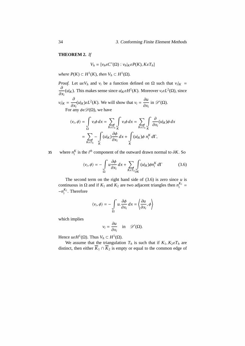
3.2. Internal Approximation ofH1(Ω). 35
the trianglesK1 andK2. By this assumption we eliminate the possibilityof a triangulation as shown in figure.
Figure 3.1:
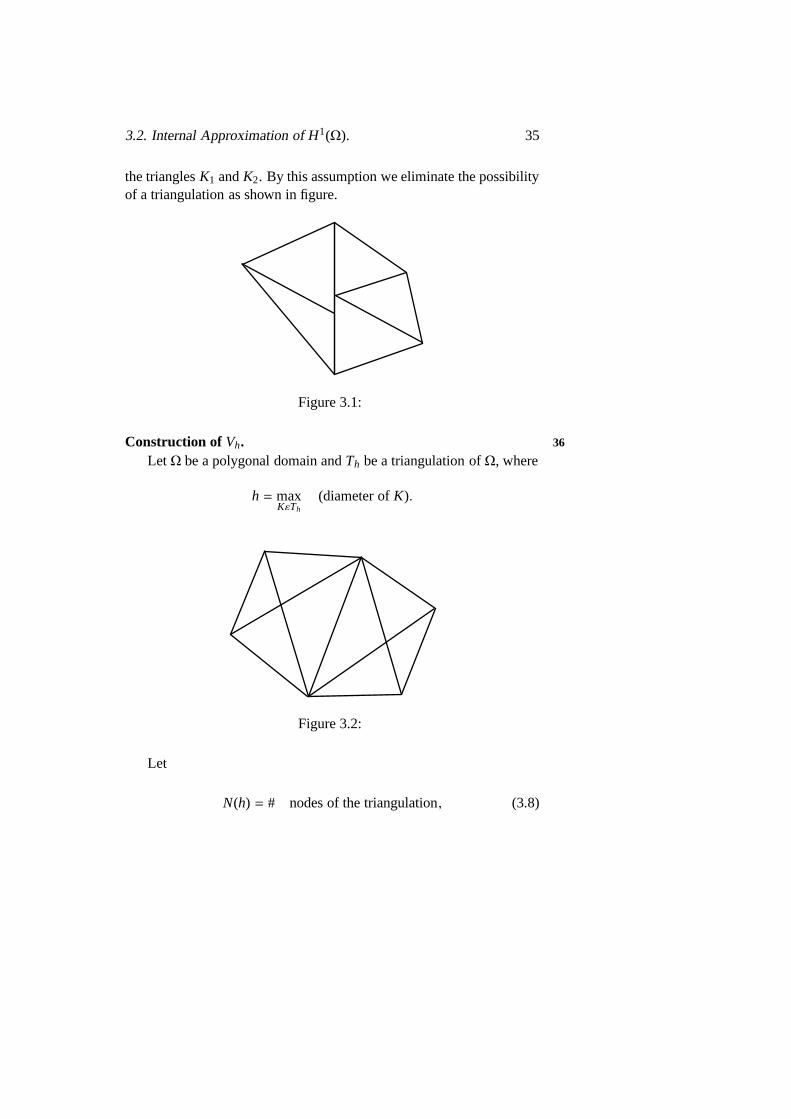
Construction of Vh. 36
LetΩ be a polygonal domain andTh be a triangulation ofΩ, where
h = maxKεTh
(diameter ofK).
Figure 3.2:
Let
N(h) = # nodes of the triangulation, (3.8)
36 3. Conforming Finite Element Methods
P(K) = P1(K) = polynomial of degree less than or equal to
1 in x and y(3.9)
LetVh = vh : vh|KεP1(K),KεTh (3.10)
We know that a polynomial of degree 1 inx andy is uniquely de-termined if its values on three non-collinear points are given. Using thiswe construct a basis forVh. A function inVh is uniquely determined ifits value at all the nodes of the triangulation is given. Let the nodes ofthe triangulation be numbered1, 2, . . . ,N(h). Let WiεVh be
wi =
1 at the ith node,
0 at other nodes.(3.11)
It is easy to see thatwi are linearly independent. IfvεVh, then37
v =N(h)∑
i=1
viwi (3.12)
wherevi the value ofv at theith node. This proves thatwi1,...,N(h) is abasis ofVh and dimension ofVh = N(h).
Moreover, Suppwi ⊂ ∪K, where the union is taken over all thetriangles whose one of the vertices is theith node.
Hence if ith node andjth node are not the vertices of a triangleK,for anyKεTh, then
Suppwi ∩ Suppw j = φ.
We will show thatVh given by (3.10) is contained inC(Ω). LetvεVh
and letK1,K2εTh be adjacent triangles. Let ‘ℓ′ be the side common toboth K1 andK2. v|K1 andV|K2 are polynomials of degree less than orequal to one inx and y. Let v1 and v2 be the extensions ofv|K1 andv|K2 to K1 and K2 respectively. ˜v1|ℓ and v2|ℓ can be thought of as apolynomial of degree less than or equal to one in asingle variableandhence can be determined uniquely if their values at two distinct pointsare known. But, by the definition ofVh in (3.10), v1|ℓ and v2|ℓ agree at38
the common vertices ofK1 andK2. Hence ˜v1|ℓ = v2|ℓ. This proves thatv is continuous acrossK1 andK2. ThusvεC(Ω). HenceVh ⊂ C(Ω).
3.3. Finite Elements of Higher Degree. 37
Using the theorem 3.2 we conclude thatVh ⊂ H1(Ω). When weimpose certain restrictions onTh, it is possible to prove thatd(u,Vh) →0 ash→ 0 whered(u,Vh) is the distance between the solutionu of (3.1)and the finite dimensional spaceVh. The reader can refer to CIARLET[9]. ThusVh “approximates”H1(Ω).
The finite element method and the finite difference scheme are the“same” when the triangulation is uniform. For elliptic problems the fi-nite element method gives better results than the finite differencescheme.
3.3 Finite Elements of Higher Degree.
DEFINITION . Let K be a triangle with vertices(ai , i = 1, 2, 3). Letthe coordinates of ai be ai j , j = 1, 2. For any xεR, the barycentriccoordinatesλi(x), i = 1, 2, 3, of x are defined to be the unique solutionof the linear system
3∑
i=1
λi ai j = x j , j = 1, 2;
3∑
i=1
λi = 1
(3.13)
Notice that the determinant of the coefficient matrix of the system39
(3.13) is twice the area of the triangleK. It is easy to see that thebarycentric coordinates ofa1, a2, a3 are (1, 0, 0), (0, 1, 0) and (0, 0, 1)respectively. The barycentric coordinate of the centroidG of K is (1/3,1/3, 1/3).
Using Cramer rule we find from (3.13) that
λ1 =
∣
∣
∣
∣
∣
∣
∣
∣
∣
x1 a21 a31
x2 a22 a32
1 1 1
∣
∣
∣
∣
∣
∣
∣
∣
∣
∣
∣
∣
∣
∣
∣
∣
∣
∣
a11 a21 a31
a12 a22 a32
1 1 1
∣
∣
∣
∣
∣
∣
∣
∣
∣

38 3. Conforming Finite Element Methods
i.e. λ1 =area of the triangle xa2a3
area of the triangle a1a2a3
Similarly, λ2 =area of the triangle a1xa3
area of the triangle a1a2a3
λ3 =area of the triangle a1a2xarea of the triangle a1a2a3
This geometric interpretation of the barycentric coordinates will behelpful in specifying the barycentric coordinates of a point. For exam-ple, the equation of the sidea2a3 in barycentric coordinates isλ1 = 0.
DEFINITION. A finite element is a triple (K,PK,∑
K), where K is a40
polyhedron, PK is polynomial space whose dimension is m and∑
K is aset of distributions, whose cardinality is m. Further
∑
K = LiεD′; i =
1, 2, . . . ,m is such that for given diεR, 1 ≤ i ≤ m, the equations
Li(p) = di , 1 ≤ i ≤ m
have a unique solution pεPK.The elements Li are calleddegree of freedom ofP.
EXAMPLE 1. (Finite Element of Degree 1). LetK = a triangle,
PK = P1(K) = Polynomials of degree≤ 1.
= Span 1, x, y
dim PK = 3,∑
K = δai : ai vertices, i = 1, 2, 3,whereδai denotes the dirac mass at the pointai . Then (K,PK ,
∑
K) is afinite element.
Figure 3.3:
3.3. Finite Elements of Higher Degree. 39
This follows from the fact thatpεP1(K) is uniquely determined if itsvalues at three non collinear points are given.
δai (λ j) = λ j(ai ) = δi j .
Henceλ j , j = 1, 2, 3, form a basis forP1(K) and if pεP1(K) then 41
p =3
∑
i=1
p(ai )λi
REMARK 1. In the definition, dimension of PK is m and we requirethat the equations
Li(p) = di , 1 ≤ i ≤ m, for given diεR have a solution. So, inexamples, to prove existence we have to prove only uniqueness. To provethe uniqueness it is enough to show that
Li(p) = 0, 1 ≤ i ≤ m, implies p≡ 0.
REMARK 2. If p jεPK , 1 ≤ j ≤ m, are such that
Li(p j) = δi j , 1 ≤ i ≤ m, 1 ≤ j ≤ m,
thenp j form a basis for PK and any pεPK can be written as
p =m
∑
i=1
Li(p)Pi .
EXAMPLE 2. (Finite Element of Degree 2). LetK = a triangle,
PK = P2(K) = Span 1, x, y, x2, xy, y2,∑
K
= δai , 1 ≤ i ≤ 3, δai j : 1 ≤ i < j ≤ 3,
whereai denote the vertices ofK andai j denote the mid point of thesideaia j .
40 3. Conforming Finite Element Methods
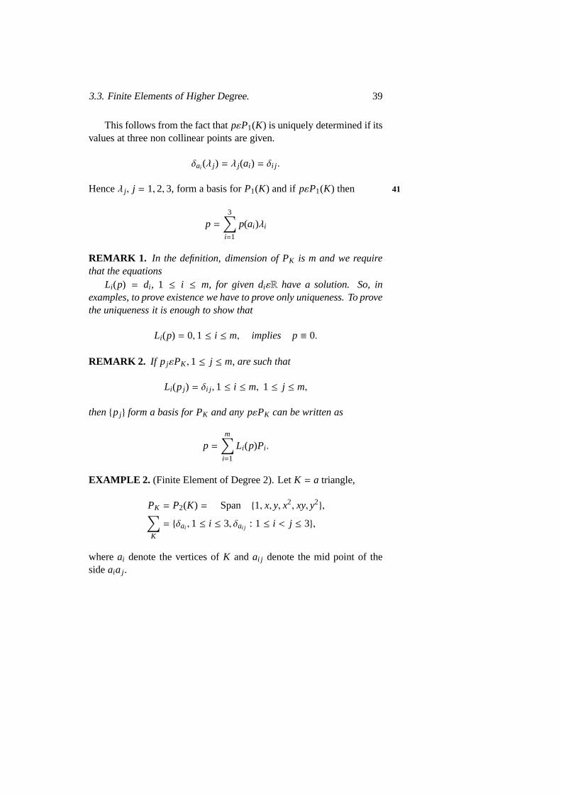
Figure 3.4:
The equations of the linesa3a2 anda13a12 areλ1 = 0 andλ1 = 1/242
respectively. Hence the functionλ1(λ1 − 1/2) vanishes at the pointsa2, a3, a12, a23, a13. The value ofλ1(λ1 − 1/2) at a1 is 1/2. Henceλ1(2λ1 − 1) takes the value 1 ata1 and 0 at other nodes.
The equations of the linesa1a3 anda2a3 areλ2 = 0 andλ1 = 0respectively. Therefore the functionλ1λ2 vanishes ata1, a2, a13, a23, a3
and takes the value 1/4 at a12. Thus 4λ1λ2 is 1 ata12 and zero at theother nodes.
Thus anypεP2(K) can be written in the form
p =3
∑
i=1
p(ai )λi(2λi − 1)+3
∑
i< ji, j=1
4p(ai j )λiλ j .
EXAMPLE 3. (Finite Element of Degree 3). LetK = a triangle,
PK = P3(K) = Span 1, x, y, x2, xy, y2, x3, x2y, xy2, y3.
Thus dimP3 = 10.
∑
K
= δai , 1 ≤ i ≤ 3; δaii j 1 ≤ i ≤ j ≤ 3, δa123.
whereai denote the vertices ofK andaii j =23
ai +13
a j .

3.3. Finite Elements of Higher Degree. 41
Figure 3.5:
It is easy to see that 43
pi = 1/2 λi(3λi − 1) (3λi − 2),
pii j = 9/2 λiλ j (3λi − 1),
p123 = 27 λ1λ2λ3,
1 ≤ i, j ≤ 3, is a basis ofP3(K).Moreover,pi is 1 at the nodeai and zero at the other nodes;pii j is 1 atthe nodeaii j and vanishes at the other nodes;p123 is zero at all nodesexcepta123 where its value is 1.
REMARK 3. In the above three examples∑
K contains only Diracmasses and not derivatives of Dirac masses. All the above three finiteelements are calledLagrange finite elements.
LetΩ be a polygonal domain and let Th be a triangulation ofΩ, i.e.Ω =
⋃
KεTh
K. Let PK = Pℓ(K) consists of polynomials of degree≤ ℓ. Let
(K,PK,∑
K) be a finite element for each KεTh. Let∑
h =⋃
KεTh
∑
K and
Vh = vh : vh|KεPK,KεTh
From the definition of finite element it follows that a function in Vh 44
is uniquely determined by the distributions in∑
h.

42 3. Conforming Finite Element Methods
REMARK 4. In the example∑
h = δai : ai is a vertex of a triangle in the triangulation. Weproved in Sec. 3.2 that Vh ⊂ H1(Ω). In this case we say that the finiteelement isconforming.
REMARK 5. The Vh so constructed above need not be contained inH1(Ω). If Vh 1 H1(Ω) we say that the finite element method isnon-conforming.
Let K be a triangle, PK = P1(K) and
∑
K
= δai j : 1 ≤ i < j ≤ 3.
Then(K,PK,∑
K) will be a finite element, but the space Vh 1 H1(Ω).
Figure 3.6:
When (K,PK,∑
K) is as in Example 2, we will prove thatVh ⊂45
C(Ω). This together with theorem 3.2 impliesVh ⊂ H1(Ω). Thus thefinite element in Example 2 is conforming.
To prove thatVh ⊂ C(Ω), let K1 andK2 be two adjacent trianglesin the triangulation.

3.4. Internal Approximation ofH2(Ω). 43
Figure 3.7:
A polynomial of degree 2 inx andy when restricted to a line in theplane is a polynomial of degree 2 in a single variable and hence can bedetermined on the line if the value of the polynomial at threedistinctpoints on the line are known. LetvhεVh. Let v1 andv2 be the continuousextension ofvh|K1 and vh|K2 to K1 and K2 respectively; ˜v1 and v2 arepolynomials of degree 2 in one variable along the common side; v1 andv2 agree at the two common vertices and at the midpoint of the commonside. Hence ˜v1 = v2 on the common side. This showsvh is continuous.HenceVh ⊂ C(Ω).
Exercise 1.Taking (K,PK ,∑
K) as in Example 3, show thatVh ⊂ H1(Ω).
3.4 Internal Approximation of H2(Ω).
In this section we give an example of a finite element which is such that 46
the associated spaceVh is contained inH2(Ω). This finite element canbe used to solve some fourth order problems. We need
THEOREM 3. If Vh = vh : vh|KεPK ⊂ H2(K), for all KεTh is con-tained in C1(Ω) then Vh is contained in H2(Ω).
The proof of this theorem is similar to that of theorem 2 of thissection.

44 3. Conforming Finite Element Methods
EXAMPLE 4. Let K be a triangle
PK = P3(K) = Span 1, x, y, x2, xy, y2, x3, x2y, xy2, y3,∑
K
=
δai ,∂
∂xδai ,
∂
∂yδai , δa123, 1 ≤ i ≤ 3
whereai are vertices ofK, a123 is the centroid ofK and
dim PK = Card∑
K
= 10.
Figure 3.8:
The arrows in the figure denote that the values of the derivatives atthe vertices are given. Using the formula
p =3
∑
i=1
(
−2λ3i + 3λ2
i − 7λ1λ2λ3
)
p(ai ) + 27λ1λ2λ3p(a123)
+
∑
1≤i< j≤3
λiλ j(2λi + λ j − 1)Dp(ai )(a j − ai) for all pεP3
47

3.4. Internal Approximation ofH2(Ω). 45
where
Dp(ai ) =
(
∂p∂x
(ai),∂p∂y
(ai )
)
.
We obtain thatp ≡ 0 if
p(ai ) = p(a123) =∂p∂x
(ai ) =∂p∂y
(ai) = 0, 1 ≤ i ≤ 3.
Hence (K,PK,∑
K) is a finite element.The correspondingVh is in C(Ω) but not inC1(Ω). This shows that
Vh 1 H2(Ω). Hence this is not a conforming finite element for fourthorder problems.
We now give an example of a finite element withVh ⊂ H2(Ω).
EXAMPLE 5. The Argyris Triangle . The Argyris triangle has 21 de-grees of freedom. Here the values of the polynomial, its firstand secondderivatives are specified at the vertices; the normal derivative is given atthe mid points.
In the figure we denote the derivatives by circles and normal deriva-tive by a straight lines.
Figure 3.9:48
We takePK = P5 = Space of polynomials of degree less than or
equal to5.
dim PK = 21;∑
K
=
δai ,∂
∂xδai ,
∂
∂yδai ,
∂2
∂x2δai ,

46 3. Conforming Finite Element Methods
∂2
∂x ∂yδai ,
∂2
∂y2δai , 1 ≤ i ≤ 3,
∂
∂nδai j 1 ≤ i < j ≤ 3
,
whereai denote the vertices ofK, ai j the midpoint of the line joiningai
anda j , and∂/∂n, the normal derivative.Let pεPK be such thatL(p) = 0, Lε
∑
K We will prove thatp = 0 inK. p is a polynomial of degree 5 in one variable along the sidea1a2. Byassumptionp, and its first and second derivatives vanish ata1 anda2.Hencep = 0 alonga1a2. Consider∂p/∂n alonga1a2. By assumption∂p/∂n vanishes ata1a2 anda12. Since the second derivatives ofp vanishata1, a2 we have the first derivatives of∂p/∂nvanish ata1 anda2; ∂p/∂nis polynomial of degree 4 in one variable alonga1a2. Hence∂p/∂n = 0alonga1a2. Sincep = 0 alonga1a2, ∂p/∂τ = 0 alonga1a2, where∂/∂τdenote the tangential derivative, i.e. derivative alonga1a2. Therefore wehavep and its first derivatives zero alonga1a2.49
Figure 3.10:
The equation ofa1a2 is λ3 = 0. Hence we can choose a line per-pendicular toa1a2 as theλ3 axis. Letτ denote the variable alonga1a2.Changing the coordinates from (x, y) to (y3, τ) we can write the polyno-mial p as
p =5
∑
i=0
λi3qi(τ)
3.4. Internal Approximation ofH2(Ω). 47
whereqi (τ) is a polynomial inτ of degree≤ 5− i. Now
∂p∂λ3=
5∑
i=1
iλi−13 qi(τ).
Sincep and its first derivatives vanish alonga1a2 we have
0 = p(0, τ) = q(τ),
0 =∂p∂λ3
(0, τ) = q1(τ)
Hence
p = λ23
5∑
i=2
λi−23 qi(τ).
Thusλ23 is a factor ofp. By taking the other sides we can prove that
λ21 andλ2
2 are also factors ofp. Thus
p = cλ21λ
22λ
23.
But λ21λ
22λ
23 is a polynomial of degree 6 which does not vanish identi-50
cally in K and p is a polynomial of degree 5. Hencec = 0. Thereforep ≡ 0 in K. Thus (K,PK ,
∑
K) is a finite element with 21 degrees offreedom.
THEOREM 4. If Vh is the space associated with the Argyris finite ele-ment, then Vh ⊂ C1(Ω).
Proof. Let K1,K2 be two adjacent finite elements in the triangulation.Let vεVh and letp1 = v|K1, p2 = v|K2. We denote the continuous exten-sions ofp1 and p2 to K1 andK2 also byp1 and p2. We have to showthat
p1 = p2,Dp1 = Dp2
along the common sideQ of K1 andK2.

48 3. Conforming Finite Element Methods
Figure 3.11:
SincevεVh, p1, p2 their first and second derivatives agree at the twocommon vertices ofK1 andK2. p1 andp2 are polynomials of degree 551
in one variable along the common sideQ. Hence, alongQ,
p1 = p2. (3.14)
Therefore∂p1
∂τ=∂p2
∂τalong Q. (3.15)
The normal derivatives∂p1
∂nand
∂p2
∂nare polynomials of degree 4
in one variable alongQ. SincevεVh,∂p1
∂n=∂p2
∂nat the two common
vertices and at the midpoint of the common sideQ. Moreover, the first
derivatives of∂p1
∂nand
∂p2
∂ncoincide at the common vertices. Hence
∂p1
∂n=∂p2
∂nalong Q. (3.16)
Equations (3.14) - (3.16) show that
p1 = p2,Dp1 = Dp2 along Q.
This proves thatv and its first derivative are continuous acrossQ.ThereforevεC1(Ω). HenceVh ⊂ C1(Ω).
Theorems 3.3 and 3.4 imply thatVh ⊂ H2(Ω). For other examplesof finite element, the reader can refer to CIARLET [9].

Chapter 4
Computation of the Solutionof the Approximate Problem
4.1 Introduction
THE SOLUTION OF THE APPROXIMATE PROBLEM. FinduhεVh 52
such that
a(uh, vh) = L(vh) ∀vhεVh, (4.1)
can be found using either iterative methods or direct methods. We de-scribe these methods in this chapter.
Let wi1≤i≤N(h) be a basis ofVh. Let A = (a(wi ,w j)) andb = (L(wi)).If a(· , · ) is symmetric, then (4.1) is equivalent to the minimizationprob-lem
J(uh) = minvhεVh
J(vh), (4.2)
whereJ(v) = 12vTAv− vTb, vεRN(h). Here we identifyVh andRN(h)
through the basiswi and the natural basisei of RN(h). uh is a solutionof (4.2) iff Auh = b. Iterative methods are applicable only whena(· , · )is symmetric.
49

50 4. Computation of the Solution of the Approximate Problem
4.2 Steepest Descent Method
Let J : RN → R be differentiable.In the steepest descent method, at each iteration we move along the
direction of the negative gradient to a point such that the functional valueof J is reduced. That is, letx•εRN be given. KnowingxnεRN, we definexn+1εRN by
xn+1= xn − λn J′(xn), (4.3)
whereλn minimizes the functional
φ(λ) = J(
xn − λJ′(xn))
(4.4)
53
In the caseJ(x) = 1/2 xTAx− xTb,
λn can be computed explicitly. It is easy to see that
J′(x) = Ax− b.
Sinceλn minimizesφ(λ), we have
φ′(λn) =(
J′(xn − λnJ′(xn)),−J′(xn))
= 0 (4.5)
Letrn= J′(xn) = Axn − b.
Then (4.5) implies
λn=
(rn, rn)(Arn, rn)
. (4.6)
For proving an optimal error estimate for this scheme we needKan-torovich’s inequality which is left as an exercise.
Exercise 1.(See LUENBERGER [30]).Prove the Kantorovich’s inequality
(Ax, x) (A−1x, x)
‖ x ‖4≤
(M +m)2
4mM(4.7)

4.2. Steepest Descent Method 51
whereA is symmetric, positive definite matrix with
m= Infx,0
(Ax, x)
‖ x ‖2> 0,M = Sup
x,0
(Ax, x)
‖ x ‖2
THEOREM 1. For any xεX the sequencexn defined by
xn+1 = xn +(rn, rn)
(rn,Arn)rn,
where 54
rn = b− Axn,
converges to the unique solutionx of Ax= b. Furthermore, defining
E(x) = ((x− x),A(x− x))
we have the estimate
‖ xn − x ‖2≤1m
E(xn) ≤1m
( M −mM +m
)2n
E(x).
Proof. We have
E(x) = (x− x,A(x− x))
= 2J(x) + (x, Ax),
where
J(x) = 1/2(x,Ax) − (b, x).
It is easy to see that
E(xn) − E(xn+1)E(xn)
=(rn, rn)2
(rn,Arn)(rn,A−1rn)≥
4Mm
(M +m)2
by Kantorovich inequality. Therefore
E(xn+1)E(xn)
≤( M −mM +m
)2
.
52 4. Computation of the Solution of the Approximate Problem
This implies
E(xn+1) ≤(M −mM +m
)2(n+1)
E(x).
From the definition ofmwe obtain 55
‖ xn − x ‖2≤1m
E(xn) ≤1m
(M −mM +m
)2.n
E(x).
The condition number ofA is defined by Cond(A) = Mm . We have
( M −mM +m
)2
∼ 1− 2mM= 1− 2
Cond(A)
If the condition number ofA is smaller, then the convergence isfaster. The steepest descent method is not a very good methodfor finiteelements, since Cond(A) ∼ C/h2 whenVh ⊂ H1(Ω).
4.3 Conjugate Gradient method
DEFINITION. The directions w1,w2εRN are said to beconjugatewith
respect to the matrix A if wT1 A w2 = 0.In the conjugate gradient method, we construct conjugate directions
using the gradient of the functional. Then the functional isminimized byproceeding along the conjugate direction. We have
THEOREM 2. Let w1,w2, . . . ,wN be N mutually conjugate directions.Let
xk+1= xk − λkwk
whereλk minimizes
φ(λ) = J(xk − λwk), λεR.
When x1εRN is given, we have56
xN+1= x∗
whereAx∗ = b.

4.3. Conjugate Gradient method 53
Proof. Letrn= −J′(xn) = b− Axn.
Sinceλk minimizesφ(λ) we have
φ(λk) = (J′(xk − λkwk),−wk) = 0.
This gives
λk=
(rk)Twk
(wk)TAwk(4.8)
Sincew1,w2, . . . ,wN are mutually conjugate directions, they are lin-early independent. Therefore there existαi , 1 ≤ i ≤ N, such that
x1 − x∗ =N
∑
k=1
αk wk.
From this, using the fact thatw j are mutually conjugate, we obtain
(x1 − x∗)TAwj= α j(w
j)T Awj .
This gives
α j =(x1 − x∗)T Awj
(w j)T Awj. (4.9)
Using induction we show that 57
αk = λk.
SinceAx∗ = b, we have
r1= Ax1 − b = A(x1 − x∗).
This shows thatα1 = λ
1.
Let αi = λi for 1 ≤ i ≤ k− 1.
From the definition ofxk we obtain
xk= x1 −
k−1∑
i=1
λiwi= x1 −
k−1∑
i=1
αi wi ,
54 4. Computation of the Solution of the Approximate Problem
(by induction hypothesis). Since
(wi)T Awk= 0 for 1≤ i ≤ k− 1,
we get(xk − x1)T Awk
= 0
This together with (4.8) and (4.9) shows that
αk = λk
Thusαk = λk for 1 ≤ k ≤ N.
The definition ofxk implies
xN+1= x1 −
N∑
i=1
λi wi= x1 −
N∑
i=1
αiwi= x∗
Algorithm for Conjugate Gradient Method
THEOREM 3. Let xεRN. Define w1= b−Ax1. Knowing xn and wn−158
we define xn+1 and wn by
xn+1= xn
+ αnwn
wn= rn+ βnwn−1,
where
rn= b− Axn, αn =
(rn,wn)(wn,Awn)
, βn =(rn, rn)
(rn−1, rn−1)
Then wn are mutually conjugate directions and xN+1 is the uniquesolution of Ax= b.
A proof of this theorem can be found in LUENBERGER [31]. Itcan be shown that
xn − xN+1 ∼(
1−√
c
1+√
c
)n
,
wherec = m/M. Thus the convergence rate in the conjugate gradi-ent method is faster than in the steepest descent method, at least forquadratic functionals.

4.4. Computer Representation of a Triangulation 55
4.4 Computer Representation of a Triangulation
1
2
3
4
5
6
7
8
5
6
81
3
4
7
2
Figure 4.1:
Let Th be a triangulation of the domainΩ. We number the nodes of the59
triangulation and the triangles inTh. Let
NS = # of nodes of Th,
NT = # of triangles in Th.
The triangulation is uniquely determined by the two matrices
Q(2, NS) = (qi j ) and ME(3, NS) = (mjk),
whereqi j denotes theith coordinate of thejth node andmjk denotes thejth vertex of thekth triangle.
The matrixME, corresponding to the triangulation in the above fig-ure is
ME =
1 1 2 2 2 6 4 62 5 4 6 5 5 6 83 2 3 4 6 8 7 7
In some problems it is better to know the boundary nodes. The arrayNG(NS) defined by
NG(i) =
1 if iεΓ
0 otherwise
56 4. Computation of the Solution of the Approximate Problem
is used for picking boundary nodes.
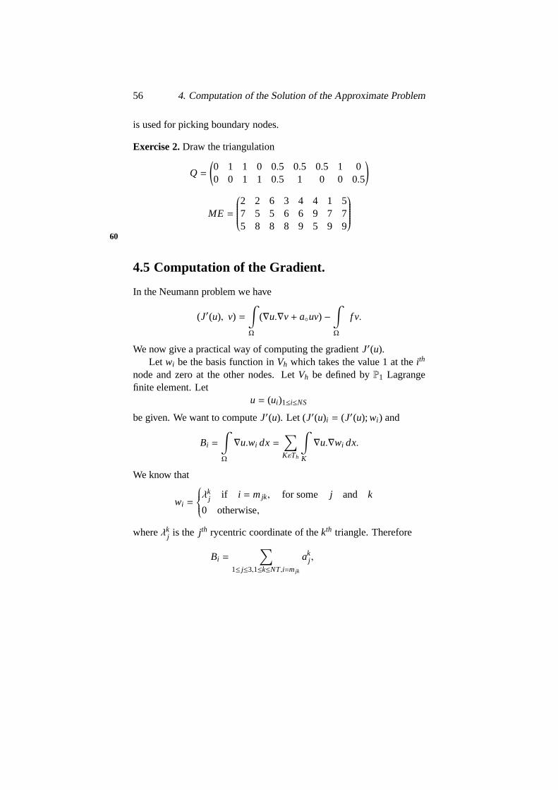
Exercise 2.Draw the triangulation
Q =
(
0 1 1 0 0.5 0.5 0.5 1 00 0 1 1 0.5 1 0 0 0.5
)
ME =
2 2 6 3 4 4 1 57 5 5 6 6 9 7 75 8 8 8 9 5 9 9
60
4.5 Computation of the Gradient.
In the Neumann problem we have
(J′(u), v) =∫
Ω
(∇u.∇v+ auv) −∫
Ω
f v.
We now give a practical way of computing the gradientJ′(u).Let wi be the basis function inVh which takes the value 1 at theith
node and zero at the other nodes. LetVh be defined byP1 Lagrangefinite element. Let
u = (ui)1≤i≤NS
be given. We want to computeJ′(u). Let (J′(u)i = (J′(u); wi ) and
Bi =
∫
Ω
∇u.wi dx=∑
KεTh
∫
K
∇u.∇wi dx.
We know that
wi =
λkj if i = mjk, for some j and k
0 otherwise,
whereλkj is the jth rycentric coordinate of thekth triangle. Therefore
Bi =
∑
1≤ j≤3,1≤k≤NT,i=mjk
akj ,
4.5. Computation of the Gradient. 57
akj =
∫
Kk
∇u.∇λkj dx, where Kk
is the triangle corresponding to thekth element. 61
Algorithm to Compute B.
Set B = 0for k = 1, 2, . . . ,NT;for j = 1, 2, 3,do Bmjk = Bmjk + ak
j .
Computation of the akj′ s.
Sinceu = (ui)1≤i≤NS and we takeP1 Lagrange finite elements, we have
u =3
∑
j=1
λkjumjk in Kk,
= ax+ by+ c, say.
Let (ξi , ηi), 1 ≤ i ≤ 3, be the coordinates of the vertices ofKk. Letw j = umjk . Thena, b are found from the equations
aξ1 + bη1 + c = w1,
aξ2 + bη2 + c = w2,
aξ3 + bη3 + c = w3,
(4.10)
as
a =(w1 − w3)(η2 − η3) − (w2 − w3)(η1 − η3)
C2(4.11)
b = − (w1 − w3)(ξ2 − ξ3) − (w2 − w3)(ξ1 − ξ3)C2
(4.12)
whereC2 = (ξ1 − ξ3)(η2 − η3) − (ξ1 − ξ2)(η1 − η3).
58 4. Computation of the Solution of the Approximate Problem
Hence∇u =(
ab
)
is determined. 62
If λkj = a j x+b jy+c, thena j andb j are got from (4.11) and (4.12) by
takingwi = δi j . Note thatC2 = 1/2 areaKk. Thenakj = C2/2 (aaj+bbj ).
4.6 Solution by Direct Methods
In Section 4.6.2 and 4.6.3 we gave algorithms to solve the equationAx=b whenA is symmetric and positive definite. WhenA is not symmetricor A is sparse, direct methods can be used to solve the equationAx= b.
4.6.1 Review of the Properties of Gaussian Elimination
The principle of Gaussian elimination is to decomposeA into a productLU whereL is lower triangular andU is upper triangular so that thelinear system
Ax= b
is reduced to solving 2 linear systems with triangular matrices
Ly = b,
Ux = y.
Each of these is very easy to solve. ForLy = b, y = (yi), y1 is givenby the first equation, hencey2 is given by the second sincey1 is alreadyknown, etc.
To decomposeA into LU, one proceeds iteratively. Let
A(k)=
(
a(k)i j
)
1 ≤ i, j ≤ N ’
be such that63
a(k)i j = 0 for 1≤ j ≤ k − 1 and i > j.
4.6. Solution by Direct Methods 59
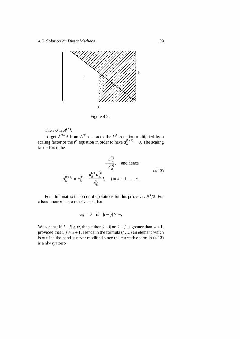
Figure 4.2:
ThenU is A(N).
To get A(k+1) from A(k) one adds thekth equation multiplied by ascaling factor of theith equation in order to havea(k+1)
ik = 0. The scalingfactor has to be
−a(k)
ik
a(k)kk
, and hence
a(k+1)i j = a(k)
i j −a(k)
ik a(k)k j
a(k)kk
i, j = k + 1, . . . , n.
(4.13)
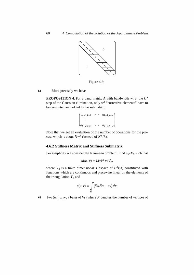
For a full matrix the order of operations for this process isN3/3. Fora band matrix, i.e. a matrix such that
ai j = 0 if |i − j| ≥ w,
We see that if|i − j| ≥ w, then either|k− i| or |k− j| is greater thanw+1,provided thati, j ≥ k+1. Hence in the formula (4.13) an element whichis outside the band is never modified since the corrective term in (4.13)is a always zero.
60 4. Computation of the Solution of the Approximate Problem
Figure 4.3:
More precisely we have64
PROPOSITION 4. For a band matrixA with bandwidthw, at thekth
step of the Gaussian elimination, onlyw2 “corrective elements” have tobe computed and added to the submatrix.
ak+1,k+1 · · · ak+1,k+w...
ak+w,k+1 · · · ak+w,k+w
Note that we get an evaluation of the number of operations forthe pro-cess which is aboutNw2 (instead ofN3/3).
4.6.2 Stiffness Matrix and Stiffness Submatrix
For simplicity we consider the Neumann problem. FinduhεVh such that
a(uh, v) = L(v)∀ vεVh,
whereVh is a finite dimensional subspace ofH1(Ω) constituted withfunctions which are continuous and piecewise linear on the elements ofthe triangulationTh and
a(u, v) =∫
Ω
(∇u.∇v+ uv) dx.
For (wi)1≤i≤N, a basis ofVh (whereN denotes the number of vertices of65
4.6. Solution by Direct Methods 61
Th), we have
a(u, v) =N
∑
i, j=1
uiai j v j ,
wherevi (respectivelyui) denote the value ofv (respectivelyu) at theith
vertex ofTh and
ai j =
∫
Ω
(∇wi ∇w j + wiw j) dx.
But this is not a practical way to compute the elementsai j of thematrix A of the linear system to be solved, since the support of thewi
involves several elements ofTh. Instead one writes
a(u, v) =∑
KεTh
∫
K
(∇u.∇v+ uv) dx.
Hence, as
u(x) =3
∑
α=1
umαKλKα (x),
v(x) =3
∑
β=1
vmβKλKβ (x),
in the elementK, where (mαK)α=1,2,3 denotes the 3 vertices of the ele-mentK andλK
α (x) the associated barycentric coordinates. One has
N∑
i, j=1
uiai j v j =
∑
KεTh
3∑
α,β=1
umαK vmβK aKαβ,
where 66
aKαβ =
∫
K
(∇λKα .∇λK
β + λKα λ
Kβ ) dx.
The matrixAK= (aK
αβ)1≤α,β≤3 is called theelement stiffness matrixof K.

62 4. Computation of the Solution of the Approximate Problem
A convenient algorithm to computeA is then the followingAssem-bling algorithm.
1. Set A = 0
2. For KεTh, computeAK and forα, β = 1, 2, 3 make
amαK ,mβK = amαK ,mβK + aKαβ.
Exercise 3.Write a Fortran subroutine performing the assembling al-gorithm (without the computation of the element stiffness matricesAK
which will be assumed to be computed in another subroutine).
4.6.3 Computation of Element Stiffness Matrices
We shall consider more sophisticated elements, e.g. the triangular, qua-dratic element with 6 nodes.
The midside points have to be included in the numbering of thever-tices to describe properly the triangulation. For each elementK, one hasto give the 6 numbers of its 6 nodes in the global numbering,
mαK , α = 1, . . . , 6.
67
The assembling algorithm of last section is still valid except thatαandβ range now from 1 to 6 and thatλK
α has to be replaced bypKα , α =
1, 2, . . . , 6, the local basis functions of the interpolation (see chapter 3).To compute the element stiffness matrix
AK=
(
aKαβ
)
α,β=1,...,6,
one introduces the mapping,
F : K → K
whereK is the triangle (0, 0), (1, 0), (0, 1). SinceF is affine, we have
F(ξ) = Bξ + b,
whereB is 2× 2 matrix andbεR2.

4.6. Solution by Direct Methods 63
Let u(ξ) = u(F(ξ)) andv(ξ) = v(F(ξ)). One has∫
K
uv dx=∫
K
uv det(B) dξ (4.14)
In the same way one has
∇u|ξ = BT ∇u|F(ξ) ,
sinceBT is the Jacobian matrix ofF. Therefore,∫
K
∇u.∇v dx=∫
K
(B−T∇u).(B−T ∇v) det(B) dξ (4.15)
Finally to compute the coefficientsaKαβ
of the element stiffness ma-
trix AK, one notices that
u(ξ) =6
∑
α=1
umαK pα(ξ),
where (pα(ξ), α = 1, . . . , 6) are the basis functions ofK which are 68
easily computed once for all. Note that
λ1 = 1− ξ1 − ξ2, λ2 = ξ1,λ3 = ξ2.
As p are polynomials (even for higher degree elements) the integralsin (4.14) and (4.15) can be computed by noticing that
∫
K
ξi1ξ
j2 dξ =
i! j!(i + j + 2)!
However, for the simplicity of the programming they are usuallycomputed by numerical integration: every integral of the type
∫
K
f (ξ) dξ
is replaced byL
∑
ℓ=1
wℓ f (bℓ)

64 4. Computation of the Solution of the Approximate Problem
where (bℓ)ℓ=1,...,L are called the nodes of the numerical integration for-mula and (wℓ)ℓ=1,...,L the coefficients.
The programming is easier since one may compute (in view of (4.14)and (4.15) only the values ofpα and∂pα/∂ξi at the pointsbℓ. For moredetails and model programs we refer to Mercier – Pironneau [32].

Chapter 5
Review of the ErrorEstimates for the FiniteElement Method
THE PURPOSE OF this chapter is to state the theorems on error esti- 69
mates which are useful for our future analysis. The proof of the theo-rems can be found in CIARLET [9].
DEFINITION. LetΩ ⊂ Rn be an open subset, m≥ 0 be an integer and1 ≤ p ≤ +∞. Then the Sobolev Space Wm,p(Ω) is defined by
Wm,p(Ω) = vεLp(Ω) : ∂αvεLp(Ω), for all |α| ≤ m.
On the space Wm,p(Ω) we define a norm‖ ‖m,p,Ω by
‖ v ‖m,p,Ω=
∫
Ω
∑
|α|≤m
|Dαv|p dx
1/p
,
and a semi norm| |m,p,Ω by
|v|m,p,Ω =
∫
Ω
∑
|α|=m
|Dαv|p dx
1/p
.
65

66 5. Review of the Error Estimates for the...
If k is an integer, then we consider the quotient space
W−k+1,p(Ω) =Wk+1,p(Ω)/pk(Ω)
with the quotient norm
‖ v ‖k+1,p,Ω= InfℓεPk
‖ v+ ℓ ‖k+1,p,Ω,
wherev is the equivalence class containing v.70
We introduce a semi norm inWk+1,p(Ω) by
|v|k+1,p,Ω = |v|k+1,p,Ω.
Then we have
THEOREM 1. (CIARLET - RAVIART). In Wk+1,p(Ω) the semi norm|v|k+1,p,Ω is a norm equivalent to the quotient norm‖ v ‖k+1,p,Ω.
Using this theorem it is easy to prove
THEOREM 2. Let Wk+1,p(Ω) and Wm,q(Ω) be such that Wk+1,p(Ω) →Wm,q(Ω) (continuous injection). Let
π ∈ L (Wk+1,p(Ω), Wm,q(Ω))
be such that for each pεPk, πp = p. Then there exists a c= c(Ω, π) suchthat for each v∈Wk+1,p(Ω)
|v− πv|m,q,Ω ≤ c|v|k+1,p,Ω.
DEFINITION. Two open subsetsΩ,Ω ofRn are said to be affine equiv-alent if there exists an affine map F fromΩ ontoΩ such that F(x) =Bx+ b, where B is a n× n non singular matrix and bεRn.
We have
THEOREM 3. LetΩ,Ω be affine equivalent with F as their affine map.Then there exist constantsc, c such that for all vεWm,p(Ω),71
|v|m,p,Ω ≤ c ‖ B ‖m |detB|−1/p|v|m,p,Ω,
67
and for all vεWm,p(Ω),
|v|m,p,Ω ≤ c ‖ B−1 ‖m |detB|1/p |v|m,p,Ω,
wherev = v • F.
If h (resp. h) is the diameter ofΩ (resp. Ω) and p (resp. p) isthe supremum of the diameters of all balls that can be inscribed inΩ(resp. Ω), then we have
THEOREM 4. ‖ B ‖≤ h/ρ and‖ B−1 ‖≤ h/ρ.
DEFINITION . Two finite elements(K, Σ, P) and (K,Σ,P) are said tobe affine equivalent if there exists an affine map Fx = Bx + b onRn,where B is an n× n non singular matrix, and bεRn such that
(i) F (K) = K
(ii) p = p = p F : pεP,
(iii) Σ = φ = F−1 φ : φεΣ
whereF−1 φ(p) = φ(p F−1).
DEFINITION . Let (K,Σ,P) be a finite element and v: K → R be a 72
smooth function on K. Then by virtue of the P-unisolvency ofΣ thereexists a unique element, say,πKv ∈ P, such thatφ(πKv) = φ(v) for allφ ∈ Σ. The functionπKv is called the P-interpolate function of v and theoperatorπK : C∞(K)→ P is called the P-interpolation operator.
Now we state an important theorem which is often used.
THEOREM 5. Let (K, Σ, P) be a finite element. Let s(= 0, 1, 2) be themaximal order of derivatives occurring inΣ. Assume that
(i) Wk+1,p(K) → Cs(K),
(ii) Wk+1,p(K) →Wm,q(K),

68 5. Review of the Error Estimates for the...
(iii) P k ⊂ P ⊂Wm,q(K),
Then there exists a constant C= C(K, Σ, P) such that for all affineequivalent finite elements(K,Σ,P) we have
|v− πKv|m,q,K ≤ C (measK)1/q−1/p hk+1K
ρmK
|v|k+1,p,K
for all v ∈ Wk+1,p(K), whereπK is a P-interpolate operator, hK is thediameter of K andρK is the supremum of diameter of all balls inscribedin K.
DEFINITION. A family(Th) of triangulations ofΩ is regular if
(i) for all h and for each KεTh the finite elements(K,Σ,P) are all73
affine equivalent to a single finite element(K, Σ, P);
(ii) there exists a constantσ such that for all Th and for each KεTh
we havehK
ρK≤ σ;
(iii) for a given triangulation Th, if
h = maxKεTh
hK ,
then h→ 0.
Exercise 1.Prove that there exists a constantC independent ofh suchthat
|p|1,k ≤ C/h |p|,K for all pεPk.
A theorem which gives a global error bound is the following.
THEOREM 6. Let us assume that
(i) πh : Hk+1(Ω)→ Vh, the restriction ofπh to Vh being the identity,
(ii) Vh ⊂ πKεTh
Pk(K),
69
(iii) Vh ⊂ Hm(Ω),74
(iv) u ∈ Hm(Ω) (regularity assumption),
Then we have‖ u− πhu ‖m,Ω≤ C hk+1−m|u|k+1,Ω,
where C is a constant independent of h and(Th) is a regular family oftriangulations.
For stating a theorem onL2 -error estimates we need the definitionof a regular adjoint problem.
DEFINITION . Let V = H1(Ω) or H1(Ω), H = L2(Ω). The adjoint
problem:
Find φεV such that
a(v, φ) = (g, v) for all vεV,
is said to be regular if
(i) for all gεL2(Ω), the solutionφ of the adjoint problem for g belongsto H2(Ω) ∩ V;
(ii) there exists a constant C such that
‖ φ ‖2,Ω≤ C|g|,Ω.
We now have
THEOREM 7. Let (Th) be a regular family of triangulations onΩwithreference finite element(K, Σ, P). Let s= 0 and n≤ 3. Suppose there75
exists an integer k≥ 1 such that uεHk+1(Ω) Pk ⊂ p ⊂ H1(K). Assumefurther that the adjoint problem is regular. Then there exists a constantC independent of h such that
|u− uh|,Ω ≤ C hk+1 |u|k+1,Ω.

70 5. Review of the Error Estimates for the...

Chapter 6
Problems with anIncompressibility Constraint
6.1 Introduction
We recall the variational formulation of the Stokes problem(see Chapter 76
2).FinduεV such that
a(u, v) = L(v) ∀ vεV,
where
a(u, v) =∫
Ω
∇u.∇v dx,
L(v) =∫
Ω
f .v dx, fε (L2(Ω))n,
andV = vε(H1
(Ω))n : div v = 0.
It is difficult to construct internal approximations ofV because ofthe constraint divv = 0. In two dimensional problem we know that
71

72 6. Problems with an Incompressibility Constraint
vεV ⇔ there existsψεH2(Ω) such that
v = rotψ,
where
rotψ =
(
∂ψ
∂x2,−
∂ψ
∂x1
)
Therefore, it seems logical that the difficulties we encountered inapproximatingH2(Ω) in a conforming way are transferred to the con-forming approximation ofV.
6.2 Approximation Via Finite Elements of Degree 1
Let Wh = vh ε (C(Ω))2 : vh|K ε(P1(K))2, for KεTh, vh = 0 on∂Ω It is77
natural to try forVh the space
vh ε Wh : div vh = 0.
But for most triangulations,Vh = 0. This is due to the fact that thenumber of equations due to the constraint divvh = 0 is greater than thenumber of degrees of freedom ofWh. In fact,
Dimension of Wh = 2 (# internal vertices).
Number of equations due to the constraint divvh = 0 is equal to numberof triangles.
HenceVh cannot be a good approximation toV. However, if the triangu-lationTh is obtained by first taking quadrilaterals and then dividingeachquadrilateral into four triangles by joining the diagonals(see figure 6.1),we obtain a ‘good space’Vh. In this case only 3 of the four equationsdiv vh = 0 are independent.

6.2. Approximation Via Finite Elements of Degree 1 73
Figure 6.1:
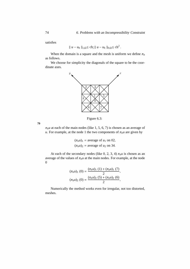
Exercise 1.Let K be a quadrilateral. Let it be divided into four triangles78
Ti , 1 ≤ i ≤ 4, by
Figure 6.2:
joining the diagonals ofK. Let vεC(K) such that
v|Ti εP1(Ti), 1 ≤ i ≤ 4. Let di = div v|Ti 1 ≤ i ≤ 4.
Then show thatd1 + d3 = d2 + d4.When the mesh isuniform, it is possible to prove convergence and
to construct an interpolation operator,
πh : V → Vh
such that‖ v− πh v ‖1,Ω≤ ch ‖ v ‖2,Ω .
Therefore the solutionvh of the approximate problem
a(uh, vh) = L(vh) ∀ vh ε Vh,
74 6. Problems with an Incompressibility Constraint
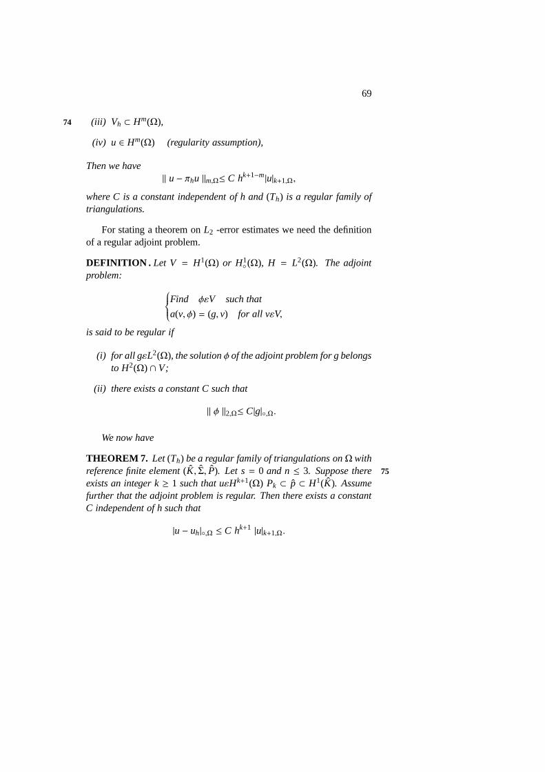
satisfies‖ u− uh ‖1,Ω≤ ch;‖ u− uh ‖0,Ω≤ ch2 .
When the domain is a square and the mesh is uniform we defineπh
as follows.We choose for simplicity the diagonals of the square to be thecoor-
dinate axes.
2 3
1 54
0
6 7
Figure 6.3:79
πhu at each of the main nodes (like 1, 5, 6, 7) is chosen as an average ofu. For example, at the node 1 the two components ofπhu are given by
(πhu)1 = average ofu1 on 02,
(πhu)2 = average ofu2 on 34.
At each of the secondary nodes (like 0, 2, 3, 4)πhu is chosen as anaverage of the values ofπhu at the main nodes. For example, at the node0
(πhu)1 (0) =(πhu)1 (1)+ (πhu)1 (7)
2,
(πhu)2 (0) =(πhu)2 (5)+ (πhu)2 (6)
2,
Numerically the method works even for irregular, not too distorted,meshes.
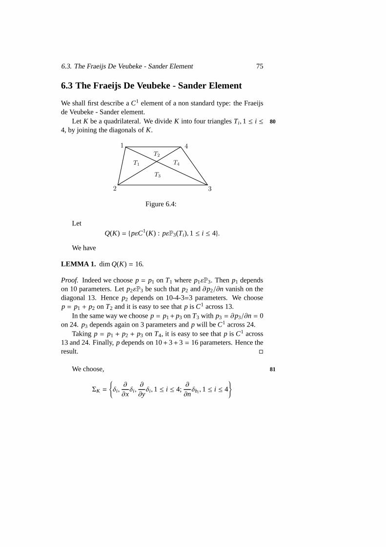
6.3. The Fraeijs De Veubeke - Sander Element 75
6.3 The Fraeijs De Veubeke - Sander Element
We shall first describe aC1 element of a non standard type: the Fraeijsde Veubeke - Sander element.
Let K be a quadrilateral. We divideK into four trianglesTi , 1 ≤ i ≤ 80
4, by joining the diagonals ofK.
1
2 3
4
Figure 6.4:
Let
Q(K) = pεC1(K) : pεP3(Ti), 1 ≤ i ≤ 4.
We have
LEMMA 1. dimQ(K) = 16.
Proof. Indeed we choosep = p1 on T1 wherep1εP3. Thenp1 dependson 10 parameters. Letp2εP3 be such thatp2 and∂p2/∂n vanish on thediagonal 13. Hencep2 depends on 10-4-3=3 parameters. We choosep = p1 + p2 on T2 and it is easy to see thatp is C1 across 13.
In the same way we choosep = p1+ p3 onT3 with p3 = ∂p3/∂n = 0on 24. p3 depends again on 3 parameters andp will be C1 across 24.
Taking p = p1 + p2 + p3 on T4, it is easy to see thatp is C1 across13 and 24. Finally,p depends on 10+ 3+ 3 = 16 parameters. Hence theresult.
We choose, 81
ΣK =
δi ,∂
∂xδi ,
∂
∂yδi , 1 ≤ i ≤ 4;
∂
∂nδbi , 1 ≤ i ≤ 4

76 6. Problems with an Incompressibility Constraint
as the set of degrees of freedom. Herebi denotes the midpoint of a sideof the quadrilateralK.
12
34
Figure 6.5:
We refer the reader to CIAVALDINI-NEDELEC [11] to prove thatthis is an admissible choice of degrees of freedom.
Let Qh denote a regular family ofquadrangulationsof the polygonaldomainΩ. Let
χh = φhεC1(Ω) : φh|KεQ(K), φh =
∂φh
∂n= 0 on ∂Ω.
Then the following result has been proved by CIAVALDINI-NEDELEC[11].
THEOREM 2. The operatorπh : H3(Ω) → χh defined by the abovechoice of degrees of freedom satisfies
‖ φ − πhφ ‖2,Ω≤ chs ‖ φ ‖s+2,Ω,
where s= 1, 2.
As a consequence of this result the spaceχh can be used to approxi-82
mate any variational problem onH2(Ω) and in particular the biharmonic
problem associated to the Stokes problem. However, as is thecase withany Hermite finite element, the programming of the Fde V-S element isdifficult and it is easier to use the corresponding element in the velocityformulation, which is quadratic.
6.4. Approximation of the Stokes Problem... 77
6.4 Approximation of the Stokes Problem ViaQuadratic Elements
Let Th be the triangulation associated toQh by dividing each quadrilat-eral ofQh into four triangles in the usual way. Let
Wh =
vh εC(Ω)2 : vh|T ε(P2(T))2,TεTh, vh = 0 on ∂Ω
andVh = vhεWh : div vh = 0.
Obviously vhεVh implies that there existsψhεχh such thatvh =
rotψh. Therefore we can state
THEOREM 3. There exists a constant c such that, for uεV ∩ Hs+1(Ω)(s= 1 or 2),
InfvhεVh
‖ u− vh ‖1,Ω≤ chs ‖ u ‖s+1,Ω .
Proof. As uεV, there existsψεHs+2(Ω) ∩ H2(Ω) such thatu = rotψ.
Then choosingvh = rotπhψ we obtain the result.
Numerically, one may solve the approximate problem: 83
find uh εVh such that
a(uh, vh) = L(vh) ∀ vh εVh,
via a penalty method.Let ε > 0 and
aε (u, v) = a(u, v) + 1/ε∫
Ω
div vdiv u dx.
The penalised problem is:
Find uh εWh such that
aε(uεh, vh) = L(vh) ∀ vh εWh.
This problem is much easier to solve. We shall see in Chapter 7that theorder of the error due to penalization is only
0(ε) :‖ uεh − uh ‖1≤ c.ε,
wherec may depend onh.

78 6. Problems with an Incompressibility Constraint
6.5 Penalty Methods.
We now come back to the case of finite elements of degree 1 wherethespaceWh is
Wh =
vh ε (C(Ω))2 : vh|K ε (P1(K))2,K ε Th, vh = 0 on∂Ω
.
The approximate problem can be taken as
Find uεh ε Wh such that
aε(uεh, vh) = L(vh) for all vh ε Wh.
We have
THEOREM 4. Assume that uεH2(Ω). Then there exists a constant c84
such that‖ uεh − u ‖21≤ c[h2(1+ 1/ε) + h+
√ε].
Hence by choosingε = h4/3 we obtain
‖ uεh − u ‖1≤ ch1/3 .
Exercise 2.Prove the above theorem.Note that the above convergence rate is very poor, which is con-
firmed by the poor numerical results obtained with this method.
6.6 The Navier-Stokes Equations.
The stationary flow of a viscous, Newtonian fluid subjected togravityloads in a bounded regionΩ of R3 is governed by the following dimen-sionless equations.
−γ∆u+3
∑
i=1
ui∂u∂xi+ ∇p = f in Ω,
div u = 0 in Ω,
u = 0 in ∂Ω,
(6.1)
6.7. Existence and Uniqueness of Solutions of... 79
whereu represents the velocity,p the pressure andf is the body force.All these quantities are in dimensionless form andγ =
µ
DVρ=
1Re where
Re is called the Reynolds number. Here is the viscosity of the fluid Da length characterizing the domainΩ,V a characteristic velocity of the85
flow andρ the density of the fluid (For more details the reader is referredto BIRD-STEWART-LIGHTFOOR ‘Transport Phenomena, Wiley Ed.p. 108).
The Reynolds number is the only parameter in the equation anditmeasures how far the Navier-Stokes model is from the Stokes model.The limiting caseγ = 0 corresponds to Euler’s equations for inviscidfluids. However, at high Reynolds number, the flow develops a bound-ary layer near the boundary. Moreover, instability and bifurcation phe-nomena can be observed which correspond physically to turbulence. Weare going to study only the flows atlow Reynolds number.
6.7 Existence and Uniqueness of Solutions ofNavier-Stokes
EQUATIONS AT LOW REYNOLDS NUMBERS. The variational for-mulation of Navier-Stokes equations is:
Find uεV such that
a(u, v) + b(u, u, v) = ( f , v) ∀vεV,(6.2)
where
a(u, v) = γ∫
Ω
∇u.∇v dx,
b(u, v,w) =∫
Ω
3∑
i, j=1
ui∂v j
∂xiw j dx
and
V = vε (H1(Ω))3 : div v = 0.

80 6. Problems with an Incompressibility Constraint
Exercise 3.Show that ifu is a solution of (6.2), then there exists a86
pεL2(Ω) such thatu, p is a solution of (6.1) in the sense of distri-butions.
Exercise 4.Show that for allu, v,wεV one has
b(u, v,w) = −b(u,w, v),
b(u, v, v) = 0.
As H1(Ω) → L4(Ω) (see LADYZHENSKAYA [27] for a proof ofthis), using Schwarz inequality twice we obtain
b(u, v,w) ≤‖ u ‖0,4‖ v ‖1‖ w ‖0,4≤ c ‖ u ‖1‖ v ‖1‖ w ‖1 .
Hence
β = Supu,v,wεV
b(u, v,w)‖ u ‖‖ v ‖‖ w ‖
< ∞.
where‖ u ‖= |u|1. We have
THEOREM 5. Assume thatβ/γ2 ‖ f ‖∗< 1. Then the problem(6.2)has a unique solution.
Proof. Let uiεV, i = 1, 2. Letvi , i = 1, 2 be the solution
a(vi ,w) + b(ui , vi ,w) = ( f ,w) ∀wε V i = 1, 2 (6.3)
Note that (6.3) is a linear problem and has a unique solution by virtue ofthe Lax-Milgram Lemma.
Choosingw = vi in (6.3) it is easy to see that87
γ ‖ vi ‖2≤ ( f , vi) ≤‖ f ‖∗‖ vi ‖ .,
Thus
‖ vi ‖≤‖ f ‖∗γ
Takingw = v2 − v1, we obtain
γ ‖ w ‖2≤ a(v2 − v1,w) = b(u1, v1,w) − b(u2, v2,w) = b(u1,−w,w)+
+b(u1 − u2, v2,w) ≤ 0+ β ‖ v2 ‖ ‖ w ‖‖ u1 − u2 ‖ .

6.7. Existence and Uniqueness of Solutions of... 81
Hence we obtain
‖ v1 − v2 ‖≤ β
γ2‖ f ‖∗‖ u1 − u2 ‖ .
Since β
γ2 ‖ f ‖∗< 1, the mappingT : ui → vi is a strict contractionand has a fixed point which obviously is the unique solution of(6.2)
REMARK 1. The proof is constructive in the sense that the algorithmun+1
= Tun gives a sequence which converges to the solution. At eachstep of this algorithm one has to solve the linearised problem (6.3).
REMARK 2. If γ2 ≥ β ‖ f ‖∗ then there exists atleast one solution to(6.2). The solution of(6.2) in this case may not be unique (see LIONS[28]). Note that problem(6.2) is equivalent to solving a non-linear88
equation F(u) = 0 where F: V → V′ is given by
F(u)(v) = a(u, v) + b(u, u, v) − ( f , v).
Let Gu be the linear operator which is tangent to F, i.e.
(Guw, v) = limθ→0
1θ
(F(u+ θw)− F(u), v) = a(w, v) + b(u,w, v) + b(w, u, v).
If Gu is not singular, then u is an isolated solution, otherwise there maybe a bifurcation. The eigenvalue problem associated to the linearisedproblem is:
Find wεV, λ ε 6C such that
a(w, v) + b(u,w, v) + b(w, u, v) = λ(w, v) v εV
and a study of this problem is of fundamental interest.We refer the reader to BREZZI-RAPPAZ-RAVIART [6] for a studyof
the convergence in the case where u is an isolated solution. In the nextsection we restrict ourselves to the case where u is unique.
82 6. Problems with an Incompressibility Constraint
6.8 Error Estimates for Conforming Method
Let Vh ⊂ V. We consider the approximate problem:
Find uh εVh such that
a(uh, vh) + b(uh, uh, vh) = ( f , vh) ∀ vh ε Vh(6.4)
Let
βh = Supu,v,wεVh
b(u, v,w)‖ u ‖‖ v ‖‖ w ‖
and89
‖ f ‖h∗= SupuεVh
( f , v)‖ v ‖
.
Then it is easy to see that (6.4) has a unique solution when
βh
γ2‖ f ‖h∗< 1.
The iterative method mentioned in Remark 1 converges for allγ satis-fying γ2 > βh ‖ f ‖h∗ Note thatβh ≤ β and‖ f ‖h∗≤‖ f ‖∗; however,JAMET-RAVIART [23] proved thatβh → β and ‖ f ‖h∗→‖ f ‖∗ ash→ 0.
THEOREM 6. Assume that
β
γ2‖ f ‖∗< 1− δ
with 0 < δ < 1; then one has
‖ u− uh ‖≤ 3/δ ‖ u− vh ‖ ∀ vh εVh.
Proof. Let wh = vh − uh. Then
γ ‖ wh ‖2≤ a(vh − u,wh) + a(u− uh,wh),
a(u,wh) = ( f ,wh) − b(u, u,wh),
a(uh,wh) = ( f ,wh) − b(uh, uh,wh),
a(u− uh,wh) = b(uh, uh − u,wh)
6.8. Error Estimates for Conforming Method 83
+b(uh − u, u,wh) ≤ β ‖ uh ‖‖ vh − u ‖‖ wh ‖ +β ‖ uh − u ‖ ‖ u ‖‖ wh ‖ since b(uh, uh − vh,wh) = 0.
But we know that
‖ u ‖≤ 1/γ ‖ f ‖∗, ‖ uh ‖≤ 1/γ ‖ f ‖∗ .
Therefore we obtain 90
‖ wh ‖2≤ (‖ vh − u ‖ +(1− δ) ‖ vh − u ‖ +(1− δ) ‖ uh − u ‖) . ‖ wh ‖ .
As
‖ u− uh ‖≤‖ u− vh ‖ + ‖ wh ‖
we get
δ ‖ wh ‖2≤ (3− 2δ) ‖ vh − u ‖‖ wh ‖ .
Hence
‖ u− uh ‖≤‖ vh − u ‖ +3− 2δδ‖ u− vh ‖ .
This gives the desired result.
An immediate consequence of Theorem 6 is that, when the solutionu of (6.2) is sufficiently regular, we obtain the same error estimate forNavier-Stokes equations at low Reynolds number as for Stokes.
The method described in Section 6.4 is probably one of the bestmethods for Navier-Stokes equations at low Reynolds number.
However, when the Reynolds number is large, a major disadvantageis that the velocity field is required to be continuous (sinceour methodis conforming) and this is not good to take into account boundary layerphenomena.
Indeed the velocity profile near the boundary has the behaviour as 91
shown in figure.

84 6. Problems with an Incompressibility Constraint
Figure 6.6:
∈ is called the thickness of the boundary layer. In fact,∈= γ1/2, so thatfor high Reynolds number, this requires a very high refinement of themesh near the boundary and therefore very expensive computer time.This can be partly avoided with mixed finite element since we shall workwith discontinuous velocity fields.

Chapter 7
Mixed Finite ElementMethods
7.1 The Abstract Continuous Problem
Let V,M,H be Hilbert spaces withV → H. The continuous problem is:92
Find u, λ εV × M such that
a(u, v) + b(v, λ) = ( f , v) ∀ v εV, (7.1)
b(u, µ) = (φ, µ) ∀ µ εM, (7.1b)
wherea(· , · ) : H × H → R andb(· , · ) : V × M → R are continuousbilinear forms andfεV′, φεM′.
Let a(· , · ) andb(· , · ) satisfy
a(v, v) ≥ α ‖ v ‖2H ∀ v εH ellipticity , (7.2)
SupvεV
b(v, µ)‖ v ‖V
≥ β ‖ µ ‖M Brezzi’s condition (7.3)
|a(u, v)| ≤ |a| ‖ u ‖‖ v ‖, |b(v, µ)| ≤ |b| ‖ v ‖‖ µ ‖. We have
THEOREM 1. If H = V then, under the above assumptions problem(7.1)has a unique solution.
85
86 7. Mixed Finite Element Methods
Proof. Let us consider the regularised problem:
a(uε, v) + b(v, λε) = ( f , v) ∀ v ε V, (7.4)
− b(uε, µ) + ε(λε, µ) = −(φ, µ) ∀ µ εM, (7.4b)
LetΦ = u, λ,Ψ = v, µεV × M. We define
Aε(Φ,Ψ) = a(u, v) + b(v, λ) − b(u, µ) + ε(λ, µ), L(Ψ) = ( f , v) − (φ, µ)
ThenAε(Φ,Ψ) is V × M coercive andL(Ψ) is a continuous, linear form93
on V × M.It is easy to see that problem (7.4) is equivalent to:
Find ΦεV × M such that
Aε(Φ,Ψ) = L(Ψ) ∀ ΨεV × M
(7.5)
By Lax-Milgram Lemma, problem (7.5) has a unique solution whichimplies that the regularized problem (7.4) has a unique solution.
Taking v = uε in (7.4), µ = λε in (7.4b) and adding and using thecontinuity of bilinear forms andH-ellipticity of a(· , · ), we get
α ‖ uε ‖2 +ε ‖ λε ‖2≤ C (‖ uε ‖ + ‖ λε ‖) , (7.6)
whereC is a constant.Since
b(v, λε) = ( f , v) − a(uε, v) ≤ (‖ f ‖∗ +|a| ‖ uε ‖) ‖ v ‖
we obtain, using Brezzi’s condition,
β ‖ λε ‖≤ SupvεV
b(v, λε)‖ v ‖
≤‖ f ‖∗ +|a| ‖ uε ‖ .
This implies‖ λε ‖≤ C (1+ ‖ uε ‖) . (7.7)
From (7.6) and (7.7) we obtain
‖ uε ‖≤ C and ‖ λε ‖≤ C,

7.1. The Abstract Continuous Problem 87
whereC is a constant. Hence there exists a subsequence∈′, u ∈ V,94
λ ∈ M, such thatu∈′ u and λ∈′ λ.
Obviouslyu, λ is a solution of (7.1).If u1, λ1 andu2, λ2 are solutions of (7.1), then
a(u1 − u2, v) + b(v, λ1 − λ2) = 0 ∀v ∈ V,
b(u1 − u2, µ) = 0 ∀µ ∈ M.(7.8)
Takingv = u1 − u2 andµ = λ1 − λ2, we obtain
α ‖ u1 − u2 ‖2≤ a(u1 − u2, u1 − u2) = 0.
Thereforeu1 = u2.
Sinceu1 = u2, using Brezzi’s condition, we obtain from (7.8) that
λ1 = λ2.
Hence the solution of (7.1) is unique.
REMARK 1. We now give an error estimate for the solution of(7.1)and the regularized problem(7.4). We have
a(u− uε, v) + b(v, λ − λε) = 0 ∀v ∈ V.
Henceβ ‖ λ − λ∈ ‖≤ |a|. ‖ u− u∈ ‖ . (7.9)
From (7.1b)and (7.4b)we obtain
b(u− u∈, µ)+ ∈ (λ∈, µ) = 0∀µ ∈ M.
Choosing v= u− u∈, µ = λ − λ∈, we get 95
α ‖ u− u∈ ‖2≤ a(u− u∈, u− u∈) =∈ (λ∈, λ − λ∈) ≤∈‖ λ∈ ‖‖ λ − λ∈ ‖
Thus, using(7.7)‖ u− u∈ ‖≤ C ∈ .

88 7. Mixed Finite Element Methods
Thus from(7.9)we get
‖ λ − λ∈ ‖≤ C ∈ .
So we obtain
‖ u− u∈ ‖= 0(∈) and ‖ λ − λ∈ ‖= 0(∈).
REMARK 2. Let B : V → M be such that
(Bv, µ)M = b(v, µ) ∀ µ ∈ M.
One has, from(7.4b)and (7.4),
λ∈ = 1/ ∈ (Bu∈ − φ),
a(u∈, v) + 1/ ∈ (Bv, Bu∈ − φ) = ( f , v) ∀ v ∈ V,
which correspond to penalization of(7.1b).
REMARK 3. We proved the existence and uniqueness of(7.1) onlyunder the assumption V= H. If V , H then we do not have a generalexistence theorem. But existence theorems for particular examples whenV , H are proved.
We now give examples of(7.1).
EXAMPLE 1. The Stokes Problem.We recall that the Stokes problem96
is:Find u, p such that
−γ∆u+ ∇p = f in Ω,
div u = 0 in Ω,
u = 0 on Γ.
Without loss of generality we can takeγ = 1. Using the standardtechnique of integration by parts we find that this corresponds to theproblem:
Findu, p ε (H1
(Ω))n × (L2(Ω)/R)
7.1. The Abstract Continuous Problem 89
such that
a(u, v) + b(v, p) = ( f , v) ∀ v ε (H1(Ω))n,
b(u, µ) = 0 ∀ µ ε L2(Ω)/R;
where
a(u, v) =∫
Ω
∇u.∇v dx,
b(v, µ) = −∫
Ω
µ div v dx.
We take
V = H = (H1(Ω))n,
M = (L2(Ω)/R).
Clearly a(· , · ) is H-elliptic, continuous and bilinear. Let us proveBrezzi’s condition,
SupvεV
b(v, λ)‖ v ‖V
= Supvε(H1
(Ω))n
−∫
Ω
λdiv v
‖ v ‖V= Sup
vε(H1 (Ω))n
< ∇λ, v >‖ v ‖V
=‖ ∇λ ‖(H−1(Ω))n≥1C‖ λ ‖L2(Ω)/R
where〈, 〉 denotes the duality between (H1(Ω))n and (H−1(Ω))n. 97
Thus Stokes problem has a unique solution.
EXAMPLE 2. The Biharmonic Problem. Let
V = H1(Ω), M = H1(Ω), H = L2(Ω).
Consider the problem:Find
u, λ ε H1(Ω) × H1(Ω)
90 7. Mixed Finite Element Methods
such that
a(u, v) + b(v, λ) = 0 ∀ v ε H1(Ω), (7.10)
b(u, µ) =∫
Ω
φµ dx ∀ µ ε H1(Ω). (7.11)
where
a(u, v) =∫
Ω
uv dx, b(v, µ) =∫
Ω
∇v.∇µ dx
andφ ε L2(Ω).Using integration by parts, we obtain from (7.10) that
∫
Ω
uv dx−∫
Ω
∆λ.v dx+∫
Γ
∂λ
∂nv dΓ = 0,
which impliesu− ∆λ = 0 in Ω,
∂λ
∂n= 0 on Γ.
(7.12)
From (7.11) we get98
− ∆u = φ. (7.13)
Thus we have, from (7.12) and (7.13), the biharmonic problem
∆2λ = 0 in Ω,
∂λ∂n = 0 on Γ,
λ = 0 on Γ.
(7.14)
In the variational form of the biharmonic equation, we notice thatV = H1(Ω) , L2(Ω) = H. It is easy to see when (7.10), (7.11) has onesolution. If a solutionλ of (7.14) is inH3(Ω)∩H2
(Ω) thenu defined by(7.13) is inH1(Ω). Moreover, one can check that thisu, λ is a solutionof (7.10), (7.11).
7.2. The Approximate Problem 91
7.2 The Approximate Problem
Let Vh ⊂ V and Mh ⊂ M be two families of finite-dimensional spacesapproximatingV andM. We shall study the approximate problem:
Finduh, λh ε Vh × Mh
such that
a(uh, vh) + b(vh, λh) = ( f , vh) ∀ vh ε Vh, (7.15)
b(uh, µh) = (φ, µh) ∀ µh ε Mh. (7.15b)
99
Exercise 1.Show that the problem (7.15) leads to solving a linear sys-tem with matrix
(
A BT
B 0
)
whereA is am×mpositive definite matrix andB is n×mmatrix wherem= dimVh andn = dim Mh.
SinceVh is finite-dimensional, the norms‖· ‖v and ‖· ‖H on Vh areequivalent, that is there exists a functionS(h) such that
‖ vh ‖v≤ S(h) ‖ vh ‖H ∀ vh ε Vh. (7.16)
We introduce the affine spaces
Zh(φ) = vh ε Vh : b(vh, µh) = (φ, µh) ∀ µh ε MhZ(φ) = v ε V : b(v, µ) = (φ, µ) ∀ µ ε M
Exercise 2.Let φ = 0. Show that (7.1) is equivalent to the problem:Find
u ε Z = Z(0) such that
a(u, v) = ( f , v) ∀ v ε Z
(7.17)
In the same way show that (7.15) is equivalent to:Find
uh ε Zh = Zh(0) such that
a(uh, vh) = ( f , vh) ∀ vh ε Zh(7.18)
92 7. Mixed Finite Element Methods
100
The present framework allows us to deal withZh 1 Z and hence wecan consider non-conforming approximations of (7.17).
We now give an error bound inH-norm.
THEOREM 2. Assuming that the continuous problem has at least onesolutionu, λ one has the error bound
‖ u− uh ‖H≤(
1+|a|α
)
infvhεZh(φ)
‖ u− vh ‖H +|b|α
S(h) infµhεMh
‖ λ − µh ‖M(7.19)
Proof. Let wh = vh − uh and we have
a(wh,wh) = a(vh − u,wh) + a(u− uh,wh)
From (7.1) and (7.15), we obtain
a(u− uh,wh) = b(wh, λh − λ) ∀ wh ε Vh.
We notice that forvhεZh(φ),
b(vh − uh, µh) = 0 ∀ µh ε Mh
and hence
a(u− uh, vh − uh) = b(vh − uh, µh − λ) ∀ vh ε Zh(φ), µh ε Mh.
Using theH-coerciveness ofa(· , · ) and the continuity ofa(· , · ) andb(· , · ) we obtain
α ‖ vh − uh ‖2H≤ |a| ‖ vh − uh ‖H‖ vh − u ‖H +|b| ‖ λ − µh ‖M‖ vh − uh ‖V≤ |a| ‖ vh − uh ‖H‖ vh − u ‖H +|b| ‖ λ − µh ‖M S(h). ‖ vh − uh ‖H
Hence101
‖ vh − uh ‖H≤|a|α‖ vh − u ‖H +
|b|α
S(h) ‖ λ − µh ‖M .
We get the desired result by noticing that
‖ u− uh ‖H≤‖ u− vh ‖H + ‖ vh − uh ‖H

7.3. Application to the Stokes Problem 93
REMARK 4. If Zh(0) ⊂ Z(0) then the error estimate(7.19)reduces to
‖ u− uh ‖H≤(
1+|a|α
)
infvhεZh(φ)
‖ u− vh ‖H , (7.20)
using the fact b(vh − uh, λh − λ) = 0 as vh − uh ε Zh(0) ⊂ Z(0).Whenφ = 0, the error estimate(7.20) is obvious, inview of exercise
2. Then(7.20)is the error bound obtained in the conforming case.
7.3 Application to the Stokes Problem
In what followsTh will denote a regular family of triangulations of thepolygonal domainΩ, ϑh will denote the set of vertices ofTh,mh the setof mid side points andEh the set of edges.
We consider the Stokes problem (example 1) whereu is the velocity 102
andλ is the pressure.We shall choose forVh a conformingP2 space and forMh a piece-
wise constant space, namely
Vh = vh ε (C(Ω))n : vh|K ε(P2(K))n,K ε Th, vh = 0 on ∂Ω
andMh = µh ε L2(Ω) : µh|K ε P0(K),K ε Th.
We notice thatdimVh = n (# internal vertices+ # internal edges) and chooseΣh
for the set of degrees of freedom in each component where
Σh = δN, N εϑh; Mγ, γ ε Eh,
Mγ(p) = 1|γ|
∫
γ
p dsdenoting theaverageon the edge.
With this choice ofΣh, the interpolation operator
πh : (H2(Ω))n→ Vh
defined by
δN(πhu) = δN(u), N εϑh;

94 7. Mixed Finite Element Methods
Mγ(πhu) = Mγ(u), γ ε Eh,
will have some nice properties. Note thatπh is defined only on a subsetof V sinceu(N) is not defined for allu in (H1
(Ω))n; πh is defined onV ∩ (H2(Ω))n since the functions in (H2(Ω))n are continuous.103
Exercise 3.Let K be a triangle.Let PK = P2(K) and
ΣK = δai , Mγi , 1 ≤ i ≤ 3,
whereai are the vertices ofK andγi are edges ofK. Mγi is defined by
Mγi (p) =1|γi |
∫
γi
p d s.
Show thatΣK is PK unisolvent.We have
LEMMA 3. One has∫
K
div (πhv) dx=∫
K
div v dx ∀ v ε (H2(Ω))n
Proof. Indeed, by Green’s formula,∫
K
div (πhv) dx=∫
∂K
(πhv.n) ds
=
∫
∂K
v.n ds
sincen is constant on each side ofK.Applying again Green’s formula we get the desired result.
Error Estimates for ‖ u − uh ‖1 If uεH2(Ω) (which is true whenΩ is104
convex) then, sinceuεZ(0) (i.e. divu = 0) andMh contains functions
7.3. Application to the Stokes Problem 95
which are piecewise constant, we have, by Lemma 3,πhuεZh(0). Hencewe obtain
infvhεZh(0)
‖ u− vh ‖1≤‖ u− πhu ‖1≤ ch ‖ u ‖2 .
If the solutionuεH3(Ω) (which is unlikely sinceΩ is a polygon) theerror bound becomes ch2 ‖ u ‖3. Indeed, the interpolation operatorπh
leaves invariant the polynomial spaceP2(K) on each elementK and theabove error bound follows from Chapter 5.
However, we have
infuhεMh
‖ λ − µh ‖0≤ ch ‖ λ ‖1,
provided that the pressureλεH1(Ω).Finally, Theorem 2 gives
‖ u− uh ‖1≤ ch(‖ u ‖2 + ‖ λ ‖1),
which is only 0(h) due to the low degree of approximation for the mul-tiplier.
Other Choices for Vh and Mh.
Let
Q(K) = P2(K) + λ1 λ2 λ3,
whereλ1λ2λ3 is called thebubblefunction. Note that the dimension of105
Q(K) is 7.The choice
Vh =
vh ε (C(Ω))2, vh|K ε (Q(K))2,K ε Th, vh = 0 on ∂Ω
Mh = ΠKP1(K)
leads to the error estimates
‖ u− uh ‖1≤ ch2, ‖ u− uh ‖0≤ ch3 .

96 7. Mixed Finite Element Methods
(See CROUZEIX - RAVIART [14].The choice
Vh =
vh ε (C(Ω))2 : vh|K ε (P2(K),K ε Th, vh = 0 on ∂Ω
Mh =
µh ε C(Ω) : µh|K ε P1(K), K ε Th
,
in which Mh contains continuous piecewise linear functions, leads to thesame error estimates. (See BERCOVIER-PIRONNEAU [3]).
This last method, due to TAYLOR-HOOD [42], is widely used byengineers.
7.4 Dual Error Estimates for u− uh
Let
V2 → V → V0
M1 → M.
We denote by‖· ‖i the norms inVi (i = 0, 2) and‖· ‖1 the norm inM1. We106
assume thatV0 ≡ V′0. (In practical applicationsV0 will be a L2 space)and thatH = V (i.e. a(· , · ) is V-coercive).
Let gεV0 andw, ψεV × M satisfy
a(v,w) + b(v, ψ) = (g, v) ∀ v ε V, (7.21)
b(w, µ) = 0 ∀ µ ε M. (7.21b)
We assume (regularity result) that
‖ w ‖2 + ‖ ψ ‖1≤ c ‖ g ‖0 (7.22)
and
infvhεZh(φ)
‖ w− vh ‖V≤ e(h) ‖ w ‖2, (7.23)
infµhεMh
‖ µ − µh ‖M≤ e(h) ‖ ψ ‖1 . (7.24)
A V0-error estimate is given by

7.4. Dual Error Estimates foru− uh 97
THEOREM 4. Under the above assumptions, we have
‖ u− uh ‖0≤ ce(h)
(
‖ u− vh ‖V + infµhεMh
‖ λ − µh ‖M)
.
Proof. We know that
‖ u− uh ‖0= SupgεV0
(g, u− uh)‖ g ‖0
(7.25)
From (7.21) we have
(g, u− uh) = a(u− uh,w) + b(u− uh, ψ) (7.26)
Moreover, we have 107
a(u− uh, vh) + b(vh, λ − λh) = 0 ∀ vh ε Vh,
a(u− uh, vh) + b(vh, λ − µh) = 0 ∀ vh ε Zh(φ), ∀ µh ε Mh, (7.27)
andb(u− uh, νh) = 0 ∀ νh ε Mh. (7.28)
From (7.26), (7.21b), (7.27) and (7.28) we obtain
(g, u− uh) = a(u− uh,w− vh) + b(w− vh, λ − µh) + b(u− uh, ψ − νh)
∀ vh ε Zh(φ),
∀ µh, νh ε Mh.
Using the continuity ofa(· , · ) andb(· , · ) we get
(g, u− uh) ≤ c (‖ u− uh ‖V‖ w− vh ‖V + ‖ w− vh ‖V‖ λ − µh ‖M ++ ‖ u− uh ‖V‖ ψ − νh ‖M) ∀ vh ε Zh(φ), ∀ µh, νh ε Mh.
Taking the infimum overvhεZh(φ) andµh, νhεMh and using (7.23),(7.24), we obtain
(g, u− uh) ≤ c[‖ w ‖2(
‖ u− uh ‖V + infµhεMh
‖ λ − µh ‖M)
+
+ ‖ u− uh ‖V‖ ψ ‖1] e(h)
Finally, using the regularity result (7.22) and (7.25) we get the de-sired result.

98 7. Mixed Finite Element Methods
Application to Stokes Problem.
We choose
V0 = (L2(Ω))n,V2 = (H2(Ω))n, M1 = H1(Ω).
From the error estimates of section 7.3, we have108
infvhεZh(0)
‖ w− vh ‖1≤ ch ‖ w ‖2
andinfµhεMh
‖ ψ − µh ‖0≤ ch ‖ ψ ‖1 .
The regularity result (7.22) is nothing but the regularity result forthe Stokes problem.
Hence applying Theorem 4, we obtainL2-error estimate.
‖ u− uh ‖0≤ ch2 (‖ u ‖2 + ‖ λ ‖1) .
7.5 Nonconforming Finite Element Method forDirichlet Problem
We recall that the variational formulation of the Dirichletproblem
−∆u = f in Ω
u = 0 on ∂Ω
(7.29)
is:Find uεH1
(Ω) such that
a(u, v) = ( f , v) ∀ v ε H1(Ω), (7.30)
where
a(u, v) =∫
Ω
∇u.∇v =∑
KεTh
∫
K
∇u.∇v,
7.5. Nonconforming Finite Element Method for... 99
( f , v) =∫
Ω
f v,
andTh is a triangulation ofΩ.109
We like to consider the nonconforming finite element approximationof (7.30), namely
FinduhεZh such that
a(uh, vh) = ( f , vh) ∀ vh ε Zh, (7.31)
whereZh = vh : vh|KεP1(K),KεTh, vh is continuous
across the midside points of internal edges,vh = 0 on∂Ω.
Notice thatZh 1 H1(Ω).
We will construct a mixed finite element which is equivalent to(7.31). Multiplying the first equation in (7.29) byvεΠ
KH1(K) and in-
tegrating we obtain, using integration by parts in each triangleK,
∑
K
∫
K
∇u.∇v−∑
K
∫
∂K
(∇u.n) v =∫
Ω
f v.
This suggests
a(u, v) =∑
K
∫
K
∇u.∇v, (7.32)
b(v, µ) = −∑
K
∫
K
(µ.n) v, (7.33)
whereµ belongs to somesuitable space.We have to construct finite-dimensional subspacesVh andMh such
that the problem
Find uh, λh ε Vh × Mh with
a(uh, vh) + b(vh, λh) = ( f , vh) ∀ vh ε Vh
b(uh, µh) = 0 ∀ µh ε Mh
(7.34)

100 7. Mixed Finite Element Methods
is equivalent to (7.31). Herea(· , · ), b(· , · ) are as in (7.32) and (7.33). 110
We takeVh = ΠKP1(K).
It is easy to see that if (µh.n) is constant and continuous along inter-nal edges, thenb(vh, µh) = 0 ∀vhεZh.
DefineQ(K) ⊂ (P1(K))2
byQ(K) = q = (q1, q2) : q1 = a+ bx, q2 = c+ by.
If αx+ βy = ℓ is the equation of an edgeγ thenq.n is constant onγ forqεQ(K), wheren is normal toγ. The set
∑
K = (q.n)(ai j ) : ai j are mid points of the sides ofK is Q(K)-unisolvent. Hence
Mh = q ε (L2(Ω))2 : q|K ε Q(K),K ε Th, div q ε L2(Ω)= q ε (L2)2 : q|K ε Q(K), K ε Th, q.n
is continuous across the edges ofTh
serves our purpose.
Exercise 4.With the above constructedVh andMh show that (7.31) and111
(7.34) are equivalent. Further show thatZh(0) = Zh.
(Recall Zh(0) = vh ε Vh : b(vh, µh) = 0 ∀ µh ε Mh)
The continuous problem corresponding to (7.34) can be obtained asfollows:
It is natural to takeV = Π
KH1(K).
Whenµ is smooth we can write
b(v, µ) = −∑
K
∫
∂K
(µ.n)v
= −∑
K
∫
K
div µ.v+∫
K
µ.∇v
7.5. Nonconforming Finite Element Method for... 101
Hence we take
M =
µ ε (L2(Ω))2 : div µ ε L2(Ω)
.
Thus the continuous problem is:
Find u, λ ε V × M such that
a(u, v) + b(v, λ) = ( f , v) ∀ v ε V,
b(u, µ) = 0 ∀ µ ε M,
(7.35)
where
a(u, v) =∑
K
∫
K
∇u.∇v.
We have the characterisation:
LEMMA 5.
Z = v ε V : b(v, µ) = 0 ∀ µ ε M = H1(Ω).
112
Proof. Let vεD(Ω). Then
b(v, µ) = −∑
K
∫
K
div µ.v+∫
K
µ.∇v
= −
∫
Ω
div µ.v+∫
Ω
µ.∇v
= −〈div µ, v〉 − 〈µ, ∇v〉= −〈div µ, v〉 + 〈div µ, v〉= 0.
Sinceb(· , · ) is continuous onV × M andD(Ω) is dense inH1(Ω) in the
‖· ‖1 norm topology, we obtain
H1(Ω) ⊂ Z
102 7. Mixed Finite Element Methods
We have to prove the other inclusion. LetvεZ. Define
vi by vi |K =∂
∂xi(v|K), ∀ K ε Th.
Then vi ε L2(Ω).
Let φεD(Ω). Then
〈v1, φ〉 =∑
K
∫
K
v1φ =∑
K
∫
K
∂v∂x1
φ
=
∑
K
−∫
K
v∂φ
∂x1+
∫
∂K
v φ n1
= −⟨
v,∂φ
∂x1
⟩
+
∑
K
∫
∂K
v φ n1.
SincevεZ, b(v, µ) = 0 ∀µεM. Takingµ = (φ, 0), we obtain113
0 = b(v, µ) = −
∑
K
∫
K
div µ.v+∫
K
∇v.µ
= −∑
K
∫
∂K
(µ.n)v since µ is smooth
= −∑
K
∫
∂K
φv n1.
Therefore,
〈v1, φ〉 = −⟨
v,∂φ
∂x1
⟩
.
Hencev1 =∂v∂x1
in D ′. Similarly we havev2 =∂v∂x2
in D ′. Therefore
vεH1(Ω). Further
0 = b(v, µ) = −∑
K
∫
∂K
(µ.n)v ∀ µ ε (H1(Ω))2 ⊂ M

7.5. Nonconforming Finite Element Method for... 103
This impliesv = 0 on∂Ω. ThusvεH1(Ω). HenceZ ⊂ H1
(Ω).If u, λ is a solution of (7.35) then Lemma 5 and the second equa-
tion in (7.35) imply thatuεH1(Ω). The first equation in (7.35) gives
that−∆u = f in D ′. Thus if u, λ is a solution of (7.35), thenu is thesolution of the Standard Dirichlet problem:
−∆u = f in Ω
u = 0 on ∂Ω,(7.36)
andλ is the Lagrange multiplier for the continuity constraint for u from 114
one element to the other; (7.35) is called theprimal hybrid formulationof the Dirichlet problem.
If u is the solution of the Dirichlet problem (7.36) thenu,−∇u is asolution of (7.35). Note that whenλ is smooth thenb(· , · ) contains onlythe trace ofλ.n on the edgesγ, so thatλ is certainly not unique and theBrezzi condition does not hold.
Error Estimates for u− uh.
We notice that the interpolation operator
πh : H2(Ω)→ Zh
such thatπhu = u at the mid side points ofTh satisfies
‖ u− πhu ‖1,K≤ ch ‖ u ‖2,K .
Therefore‖ u− πhu ‖V≤ ch ‖ u ‖2 . (7.37)
On the other hand, we define
π′h : (H1(Ω))2→ Mh
onγ by
(π′hµ).n =1|γ|
∫
γ
λ.n
We now state a theorem whose proof can be found in RAVIART-THOMAS [38].

104 7. Mixed Finite Element Methods
THEOREM 6. There exists a constant c such that 115
‖ µ − π′hµ ‖M≤ ch(‖ µ ‖1 + ‖ div µ ‖1) , (7.38)
‖ π′hµ ‖M≤ c ‖ µ ‖1 .Using Theorem 2,(7.37)and (7.38)we obtain
‖ u− uh ‖V≤ ch ‖ u ‖2 . (7.39)
The dual error estimate of section 7.4 together with(7.39)gives
‖ u− uh ‖0≤ ch2 ‖ u ‖2 (7.40)
REMARK 5. In practice, one solves the approximate problem;
Find uh ε Zh such that
a(uh, vh) = ( f , vh) ∀ vh ε Zh,
since Zh is a simple finite element space. The fact that Zh 1 H1(Ω)
has no importance for practical purposes. The same Zh can be usedto approximate the Stokes problem. One chooses Vh = (Zh)2 (for thevelocities) and piecewise constant pressure; i.e. Mh as in section 7.3.For the error analysis we refer the reader to CROUZEIX-RAVIART [14].
REMARK 6. Other primal hybrid finite elements can be obtained withother choices for VhE Mh, some of them giving other well known non-conforming finite elements. (See RAVIART-THOMAS [37]).
7.6 Approximate Brezzi Condition
We assume that the approximate Brezzi condition116
SupvhεVh
b(vh, µh)‖ vh ‖V
≥ γ ‖ µh ‖M ∀ µh ε Mh, (7.41)
whereγ is independent ofh, holds. The approximate Brezzi conditionguarantees a unique solution for the approximate problem. Notice thatthe continuous Brezzi condition need not imply the approximate Brezzicondition.
We have the following result:

7.6. Approximate Brezzi Condition 105
THEOREM 7. Under the assumption(7.41) there exists a constant c1
such thatInf
vhεVh(φ)‖ u− vh ‖V≤ c1 Inf
whεVh
‖ u− wh ‖V (7.42)
Proof. We will show that for eachwhεVh there exists avhεZh(φ) suchthat
‖ u− vh ‖≤ c ‖ u− wh ‖,
wherec is a constant. This will imply (7.42).Let whεVh. Let yh, νhεVh × Mh be the solution of
(yh, vh)V + b(vh, νh) = 0 ∀ vh ε Vh,
b(yh, µh) = b(u− wh, µh) ∀ µh ε Mh.
Using the approximate Brezzi condition and the continuity of b(, ), 117
it is easy to prove that
‖ νh ‖M ≤ 1/γ ‖ yh ‖V,‖ yh ‖V ≤ |b|/γ ‖ u− wh ‖V .
Let vh = yh + wh. Then
b(vh, µh) = b(u− wh, µh) + b(wh, µh)
= b(u, µh).
HencevhεZh(φ). Further
‖ u− vh ‖V ≤‖ u− wh ‖V + ‖ yh ‖V≤ (1+ |b|/γ) ‖ u− wh ‖V .
Hence the theorem.
We now give an error estimate for the multiplier.
THEOREM 8. If (7.41)holds then one has the error estimate
‖ λ − λh ‖M≤ c
(
‖ u− uh ‖H + InfµhεMh
‖ λ − µh ‖M)
(7.43)

106 7. Mixed Finite Element Methods
Proof. We have
b(vh, λh − µh) = b(vh, λh − λ) + b(vh, λ − µh)
= a(u− uh, vh) + b(vh, λ − µh)
From (7.41) we obtain
γ ‖ λh − µh ‖M ≤ SupvhεVh
b(vh, λh − µh)‖ vh ‖V
≤ |a|c ‖ u− uh ‖H +|b| ‖ λ − µh ‖M . (7.44)
Further118
‖ λ − λh ‖M≤‖ λ − µh ‖M + ‖ λh − µh ‖M (7.45)
From (7.44) and (7.45) we obtain (7.43).
We now give a practical way of verifying the approximate Brezzicondition (7.41).
LEMMA 9. If b(· , · ) satisfies continuous Brezzi condition and if
Λh : V → Vh
is such that
b(v− Λhv, µh) = 0 ∀ µh ε Mh (7.46)
(in factΛh maps Z(φ) into Zh(φ)) and
‖ Λhv ‖V≤ c ‖ v ‖V, (7.47)
then(7.41)holds withγ = β/c.
Exercise 5.Prove Lemma 9.For further details see FORTIN [18].

7.7. Dual Error Estimate for the Multiplier 107
7.7 Dual Error Estimate for the Multiplier
This section is an analogue to Section 7.4. We assume thatV2 → V and119
M3 → M → M0. Further, we assume thatM′0 = M0 and that forgεM0,the problem:
Find w, ψ εV × M such that
a(v,w) + b(v, ψ) = 0 ∀ v εV (7.48)
b(w, µ) = (g, µ) ∀ µ ε M (7.48b)
has one solution such that
‖ w ‖2 + ‖ ψ ‖3≤ c ‖ g ‖0 (7.49)
We also assume that
InfvhεVh
‖ w− vh ‖V ≤ e(h) ‖ w ‖2, (7.50)
InfµhεMh
‖ ψ − µh ‖M ≤ ε(h) ‖ ψ ‖3 . (7.51)
Here‖ ‖0, ‖ ‖2, ‖ ‖3 denote the norms inM0,V2,M3 respectively. Thedual error estimate is given by
THEOREM 10. One has
‖ λ − λh ‖0≤ ce(h) (‖ λ − λh ‖M + ‖ u− uh ‖H)+
+ c ε(h)
(
S(h) ‖ u− uh ‖H + InfyhεVh
(‖ u− yh ‖V +S(h) ‖ u− yh ‖H)
)
(7.52)
Proof. We have
‖ λ − λh ‖0= SupgεM0
(g, λ − λh)‖ g ‖0
and 120
(g, λ − λh) = b(w, λ − λh)
= b(w− vh, λ − λh) − a(u− uh, vh).
108 7. Mixed Finite Element Methods
where the above is obtained from (7.1) and (7.15). Usingb(u−uh, νh) =0 ∀ νh ε Mh and (7.48), we obtain
(g, λ − λh) = b(w− vh, λ − λh) + a(u− uh,w− vh) + b(u− uh, ψ − νh)
This implies,
(g, λ−λh) ≤ c(e(h)(‖ λ−λh ‖M + ‖ u−uh ‖H)+ ‖ u−uh ‖V ε(h)) ‖ g ‖0 .
Here (7.49) - (7.51) are used.To estimate‖ u− uh ‖V, we remark that
‖ u− uh ‖V ≤‖ u− yh ‖V + ‖ yh − uh ‖V,‖ yh − uh ‖V ≤ S(h) ‖ yh − uh ‖H
≤ S(h)(‖ yh − u ‖H + ‖ u− uh ‖H).
Finally,
‖ λ − λh ‖0≤ c[e(h)(‖ λ − λh ‖M + ‖ u− uh ‖H)+
ε(h)(S(h) ‖ u− uh ‖H + InfyhεVh
(‖ u− yh ‖V +S(h) ‖ u− yh ‖H))]
7.8 Application to Biharmonic Problem
We shall now study a finite element approximation to the biharmonic121
problem. (Example 2, Section 7.1). We recall that in the variationalformulation of the biharmonic problem
∆2λ = −φ in Ω,
λ =∂λ
∂n= 0 on ∂Ω,
we have
V = H1(Ω), M = H1(Ω),H = L2(Ω),

7.8. Application to Biharmonic Problem 109
a(u, v) =∫
Ω
uv dx, b(v, µ) = −∫
Ω
∇v.∇µ
and f = 0.In the terminology of hydrodynamicsλ = ψ is called thestream
functionandw = −∆ψ = u is called theVortexfunction.For bothVh and Mh we shall use standard Lagrange finite element
space of degreek:
Vh =
vh ε C(Ω) : vh|K ε Pk(K), ∀ K ε Th
andMh = µh ε Vh : µh = 0 on ∂Ω .
We immediately notice that the approximate Brezzi condition (7.41)holds. Indeed,
SupvhεVh
∫
Ω
∇vh.∇µh
‖ vh ‖1≥
∫
Ω
|∇µh|2
‖ µh ‖1≥ γ ‖ µh ‖1 .
sinceMh ⊂ Vh. Hereγ is the constant occurring in Poincare’s inequality.122
Moreover, assuming that the triangulation satisfies the uniformitycondition
h ≤ cρK , ∀ K ε Th,
whereρK denotes the diameter of the largest ball included inK andc isa constant independent ofh, one always has
‖ v ‖1≤c
minρKKεTh
‖ vh ‖0 .
Therefore one has the inverse inequality‖ vh ‖1≤ ch ‖ vh ‖0 which gives
an evaluation ofS(h).We can state a convergence result fork > 2.
THEOREM 11. If λεHm+1(Ω) and uεHm(Ω) then one has
‖ u− uh ‖0 + ‖ λ − λh ‖1≤ chm−1 (‖ u ‖m + ‖ λ ‖m+1)
for m= 2, . . . , k and
‖ λ − λh ‖0≤ chm (‖ u ‖m + ‖ λ ‖m+1)

110 7. Mixed Finite Element Methods
The above result is a consequence of Theorems 2, 7, 8, 10. We notethat the result is not optimal since with polynomials of degree k, weshould get an error bound inhk for ‖ λ − λh ‖1 provided thatλεHk+1.
These results have been recently improved by SCHOLTZ [41] who123
is able to give an error estimate in the casek = 1.Note that the matrixA of the bilinear form onVh has to be computed
exactly in this case. (The use of a 1-point formula for the computationof
∫
K
uv dxleads to a diagonal matrixA but there is no convergence).
REMARK 7. Due to the inclusion Mh ⊂ Vh, the matrix B of the bilinearform b(· , · ) on Vh × Mh has the particular form B= (B1, B2) where B1
is the matrix of b(· , · ) on Mh × Mh and therefore B1 is invertible. Thelinear system corresponding to the approximate problem canbe writtenas
A1 A2 BT1
AT2 A3 BT
2B1 B2 0
u1
u2
λ
=
00φ
One can eliminate u1 from the last equation(u1 = −B−11 B2 u2) andλ
from the first one. This gives a linear system of equations in u2 whichcan be solved by any of the standard method.
The advantage is that the size of the linear system is p× p where pis the number of boundary points which is relatively small.
7.9 General Numerical Methods for the Solution ofthe Approximate Problem
As we have noticed in Exercise 1, the approximate problem is equivalent124
to solving(
A BT
B 0
) (
uλ
)
=
(
fφ
)
(7.53)
where the matrix on the left is invertible (provided thatB has a maxi-mal rank, i.e. the approximate Brezzi condition holds at least for γ de-pendent onh) and symmetric ifa(· , · ) is symmetric but not positive.
7.9. General Numerical Methods for the... 111
Alternatively one can use the matrix
(
A BT
−B 0
)
which is positive but not symmetric.
a) Solution of the Linear System(7.53)by Direct Methods. TheGaussian elimination of (7.53) can be performed without pivot-ing. However, due to storage considerations, it is often much bet-ter to permute rows and columns to get a band matrix after a suit-able ordering of the unknowns. (For finite elements, we ordertheunknowns following the ordering that we give to the associatednodes, with no distinction betweenλi ’s andui ’s). In this case astrategy of partial pivoting may be necessary.
b) Solution of the Approximate Problem by Penalty Methods. 125
First solve
(A+ 1/ ∈ BTB) u∈ = f + 1/ ∈ BT φ,
and then findλ∈ = 1/ ∈ (Bu∈ − φ).
If Bhas maximal rank the error is only 0(∈) (see proof of Theorem1), which is certainly small compared to the discretizationerror if∈= 10−4 or 10−6.
However, the condition number of the matrix
A+ 1/ ∈ BTB
might be quite big and it is wise in such a case to use direct meth-ods and then to compute explicitly the matrixBTB, which is easyonly if
Mh = πK(Pk(K))d
for some positivek andd; in otherwords, no continuity require-ments has to be asked forλh between two elements. (ThenBTB

112 7. Mixed Finite Element Methods
can be computed by assembling some stiffness matrices). Other-wise the computation ofBTB is too costly. Note that this methodis possible even ifB has not a maximal rank (and the error is thenonly 0(
√∈)).
c) Solution of the Problem by Iterative Methods. The conjugategradient method has been successfully extended to the case ofmatrices such as (7.53) by PAIGEand SAUNDERS [35].126
Another way of applying the conjugate gradient method isto notice thatu can be eliminated from (7.53):
u = A−1 f − A−1BTλ.
Then we getCλ = b
whereC = BA−1 BT, b = BA−1 f − φ.
As C is symmetric and positive definite (ifa(· , · ) is sym-metric) then the conjugate gradient method can be applied tothematrix C, but one has never to compute the matrix C explicitly.(This is too costlyunless Ais block diagonal and thereforeVh isa finite element space with no continuity requirements between 2elements. LetAK denote the element matrix ofa(· , · ) on K andBK that of b(· , · ); the matrixC is computed by assembling theBKA−1
K BTK ’s. This is the case for hybrid elements).
Indeed what one needs for the conjugate gradient methodis to be able to computey = Cz for any column vectorz and thisis done in the following way:
Compute z1 = BT ;
Solve Az2 = z1 ;
Compute y = Bz2 .
Note that it is not necessary forB to have maximal rank.127

7.10. Equilibrium Elements for the Dirichlet Problem 113
7.10 Equilibrium Elements for the Dirichlet Prob-lem
Let us consider the following problem:Find u, λ such that
u− ∇λ = 0 in Ω
div u = φ in Ω
λ = 0 in ∂Ω
(7.54)
If u, λ is a solution of (7.54) thenλ is the solution of the StandardDirichlet Problem:
∆λ = φ in Ω
λ = 0 on ∂Ω(7.55)
Multiplying (7.54) byv ∈ (L2(Ω))2 and using integration by partswe obtain an equivalent problem:
Find u, λ ∈ (L2(Ω))2 × H1(Ω) such that
a(u, v) + b(v, λ) = 0 ∀ v ∈ (L2(Ω))2,
b(u, µ) =∫
Ω
φµ ∀ µ ∈ H1(Ω),
where
a(u, v) =∫
Ω
u.v dx,
b(v, µ) = −∫
Ω
v.∇µ dx.
If Mh = C(Ω) ∩ πKPk(K) then a natural choice forVh is 128
Vh = πK(Pk−1(K))2.
Note that the operator∇mapsMh into VH. This implies that the approx-imate Brezzi condition holds.
114 7. Mixed Finite Element Methods
Problem (7.54) can be formulated in another way also.Find u, λ ∈ H(div, Ω) × L2(Ω) such that
∫
Ω
uv+∫
Ω
λdiv v = 0 ∀ v ∈ H (div, Ω),
∫
Ω
µ div u = (µ, φ) ∀ µ ∈ L2(Ω),
whereH (div,Ω) = v ∈ (L2(Ω))2 : div v ∈ L2(Ω).
We notice that
a(u, v) =∫
Ω
u.v dx
is coercive onH = (L2(Ω))2.
To prove thatb(· , · ) satisfies Brezzi condition, we use the fact thatifµεL2(Ω) then the solutionψ of the Dirichlet problem:
∆ψ = µ in Ω
ψ = 0 on ∂Ω,
satisfies‖ ψ ‖1≤ c ‖ µ ‖0.129
Therefore,
Supvε(L2(Ω))2
∫
Ω
µ. div v
‖ v ‖V≥
∫
Ω
µ div (∇ψ)
‖ ∇ψ ‖V≥
∫
Ω
µ2 dx
c ‖ µ ‖0=
1c‖ µ ‖0 .
As approximate spaces, we choose
Vh = v ε V : v|K ε Q(K), v.n is
continuous across the sides ofTh.
(See Section 7.5 for the definition ofQ(K)).
Mh = πKP0(K).
7.10. Equilibrium Elements for the Dirichlet Problem 115
As div : Vh → Mh, we see thatZh(0) ⊂ Z(0). (Hence the nameequi-librium elements:uh will satisfy equilibrium equations divuh = φ for φpiecewise constant).
We may then apply the error estimate derived in Section 7.2 anduse the improvement given in Remark 4, sinceZh(0) ⊂ Z(0). We shallchoosevh = π
′hvwhereπ′h is the interpolation operator defined in Section
7.5.Indeed, we have
∫
γ
(π′h v).n ds=∫
γ
v.n ds for each edge γ of Th.
Therefore, 130
∫
Ω
µh div π′h v =∑
K
∫
∂K
(π′hv).nµh dΓ
=
∑
K
∫
∂K
(v.n) µh dΓ =∫
Ω
µh div v dx ∀ µh ε Mh.
This shows thatvεZ(φ)⇒ π′h v ε Zh(φ).Finally we get
‖ u− uh ‖0≤ c ‖ u− π′h u ‖0≤ ch,
where we have used the estimate given in Theorem 6.To get an error estimate for‖ λ − λh ‖0, we shall make use of the
results in Section 7.6 and construct the operatorπh occurring in Lemma9.
Let v in V be given andφ satisfy
∆φ = div v in Ω,
φ = 0 on ∂Ω.
LetΛ : V → (H1(Ω))2
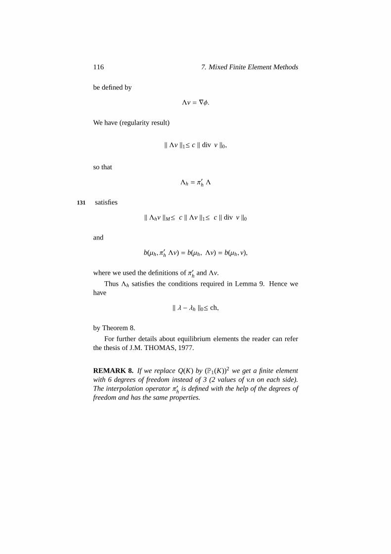
116 7. Mixed Finite Element Methods
be defined by
Λv = ∇φ.
We have (regularity result)
‖ Λv ‖1≤ c ‖ div v ‖0,
so that
Λh = π′h Λ
satisfies131
‖ Λhv ‖M≤ c ‖ Λv ‖1≤ c ‖ div v ‖0
and
b(µh, π′h Λv) = b(µh, Λv) = b(µh, v),
where we used the definitions ofπ′h andΛv.
ThusΛh satisfies the conditions required in Lemma 9. Hence wehave
‖ λ − λh ‖0≤ ch,
by Theorem 8.
For further details about equilibrium elements the reader can referthe thesis of J.M. THOMAS, 1977.
REMARK 8. If we replace Q(K) by (P1(K))2 we get a finite elementwith 6 degrees of freedom instead of 3 (2 values of v.n on each side).The interpolation operatorπ′h is defined with the help of the degrees offreedom and has the same properties.
7.10. Equilibrium Elements for the Dirichlet Problem 117
Figure 7.1:
In fact,π′h is defined by 132
∫
γ
p(π′hv).n ds=∫
γ
p(v.n) ds ∀ p ε P1(γ)
However, the error estimates now become
‖ u− uh ‖0 ≤ ch2
‖ λ − λh ‖0 ≤ ch
REMARK 9. The present finite element method can be extended to theelasticity equation where v represents the stress tensorσi j . The difficultylies in the required symmetry ofσi j but can be surmounted. See C.JOHNSON-B. MERCIER [25] and AMARA-THOMAS[2].
REMARK 10. Aposteriori Error Estimate. Let us consider the fol-lowing optimization problem:
Inf J(v, µ)
v ε Z(φ)
µ ε M
where J(v, µ) = 1/2 ‖ v − ∇µ ‖2. Clearly the optimal value is zero andcorresponds to v= u andµ = λ solution of (7.54). Since vεZ(φ), we

118 7. Mixed Finite Element Methods
also have
J(v, µ) = 1/2 ‖ ∇µ ‖2 +(φ, µ) + 1/2 ‖ v ‖2 .
Since J(u, λ) ≤ J(vh, λ) ∀ vh ε Z(φ), we obtain
1/2 ‖ u ‖2≤ 1/2 ‖ vh ‖2 .
Adding133
1/2 ‖ ∇µh ‖2 +(φ, µh)
to both sides, whereµhεM, we get
J(u, µh) ≤ J(vh, µh) ∀ µh ε M, vh ε Z(φ).
That is,‖ ∇(λ − µh) ‖0≤‖ vh − ∇µh ‖0 ∀ vh ε Z(φ).
Suppose thatµh is a solution of Dirichlet problem with a conformingfinite element method, then an upper bound for the error in theenergynorm is given by
‖ vh − ∇µh ‖0
wherevh ε Zh(φ)
is arbitrary. One can choose vh = uh, a solution of the present equilib-rium finite element approximation to Dirichlet problem.
7.11 Equilibrium Elements for the Plate Problem
We recall that the equations of the plate problem are:Findσi j ,w such that
σi j = λ∆wδi j + 2µ∂2w
∂xi ∂x jin Ω ⊂ R2 (7.57)
∂2σi j
∂xi ∂x j= f in Ω (7.57b)

7.11. Equilibrium Elements for the Plate Problem 119
w = 0 on∂Ω (7.57c)
and134
∂w∂n = 0 on ∂Ω clamped case
σi j ni n j = 0 on ∂Ω simply supported plate problem(7.57d)
The summation convention is used in the above equations.
Exercise 6.Show that (7.57) is equivalent to a biharmonic problem forwalone, and write the variational formulation of that biharmonic problem.Notice that in the clamped case several bilinear forms may bechosenunlike in the simply supported case.
It is easy to check that (7.57) is equivalent to
ασi j + β(σkk) δi j =∂2w
∂xi ∂x j, (7.58)
where
α = 1/2µ and β =−λ
2µ(2λ + 2µ).
Let
a(σ, τ) =∫
Ω
(ασi jτi j + β(σkk)(τℓℓ)) dx
and
Dw =
(
∂2w∂xi ∂x j
)
.
Then problem (7.57) is equivalent to: 135
Find σε (L2(Ω))4s, w ε H2
(Ω) such that
a(σ, τ) −∫
Ω
τ Dw dx= 0 ∀ τε (L2(Ω))4s,
∫
Ω
σ Dv =∫
Ω
f v dx. ∀
v ε H2(Ω).
v ε H2(Ω) ∩ H1(Ω).
120 7. Mixed Finite Element Methods
(L2(Ω))4s denotes the set of symmetric 2× 2 tensors which are inL2(Ω).
However, as noticed in Section 7.10, to approximate this problem inthe usual way does not represent any progress on the usual conformingapproximations since one has to approximateH2
(Ω).We have, by Green’s formula,
∫
K
τ Dv =∫
K
τi j∂2v
∂xi∂x jdx
=
∫
∂K
τi j n j∂v∂xi−
∫
K
∂τi j
∂x j
∂v∂xi
dx
Since∂v∂xi=∂v∂n
ni +∂v∂s
si
where (si) are the components of the unit tangent vector, we obtain
∫
Ω
τ Dv =∑
K
∫
∂K
Mn(τ)∂v∂n+
∑
K
∫
∂K
Mns(τ)∂v∂s−
∫
K
∂τi j
∂x j
∂v∂xi
dx
HereMn(τ) = τi j ni n j , Mns(τ) = τi j n j si .
We define136
b(τ, v) =∑
K
∫
K
∂τi j
∂x j
∂v∂xi
dx−∫
∂K
Mns(τ)∂v∂s
ds
,
V = τ : τ|K ε (H1(K))4s, K ε Th,Mn(τ)
is continuous across inter element boundaries.Then
∫
Ω
τ Dv = b(v, τ) ∀ v ε H2(Ω), τ ε V.
In fact,b(· , · ) is continuous overV×M whereM =W1,p (Ω)(p > 2)
so that (7.57) (clamped case) is equivalent to:

7.11. Equilibrium Elements for the Plate Problem 121
Find σ,w ε V × M such that
a(σ, τ) + b(τ,w) = 0 ∀ τ ε V,
b(σ, v) = −( f , v) ∀ v ε M.(7.59)
We takeH = (L2(Ω))4
s.
The Brezzi condition holds only onH1(Ω), since ifv is smooth and
τi j = vδi j , then
Mns(τ) = v (δi j n j si) = 0,
Mn(τ) = v,
and 137
b(v, τ) =∫
Ω
|∇v|2 dx≥ α ‖ v ‖21≥ c ‖ v ‖1‖ τ ‖ .
For the proof of existence of solutions of (7.59) and modifiederrorestimates see BREZZI-RAVIART [7].
We choose
Vh = τ : τ ε (P(K))4s, K ε Th, Mn(τ) is continuous.
Sincev ε W1,p
(Ω) ⊂ C(Ω)
we find that after integration by parts on each of∂K, b(τ, v) involvesonly the values ofv at the vertices ofTh:
b(τ, v) =∑
K
∫
∂K
Mns(τ)∂v∂s=
∑
N
R(τ,N) v(N) ∀ τ ε Vh. (7.59b)
Notice that only the value ofv at the vertices has to be taken; there-fore, we choose
Mh =
vh ε C(Ω) : vh|K ε P1(K),K ε Th, vh = 0 on ∂Ω

122 7. Mixed Finite Element Methods
so that, ifτεVh, then
b(τ, vh) = 0 ∀ vh ε Mh⇒ b(τ, v) = 0 ∀ v ε M.
Therefore,Zh(0) ⊂ Z(0). Hence
‖ σ − σh ‖0≤ InfτhεZh(− f )
‖ σ − τh ‖ .
Hereσh,whεVh × Mh is the solution of the approximate problem.
a(σh, τh) + Σ R(τh,N) wh(N) = 0 ∀ τh ε Vh,
Σ R(σh,N) vh(N) = −( f , vh) ∀ vh ε Mh(7.60)
138
Interpolation Operator.
The interpolation operator
πh : (H1(Ω))4→ Vh
is defined by∫
γ
Mn(πh, σ) ds=∫
γ
Mn(σ) ds,
for each edgeγ of the triangulation.We have the estimate
THEOREM 12. There exists a constant c independent of h such that
‖ πhv ‖V≤ c ‖ v ‖V (7.61)
and
‖ πhv− v ‖0,Ω≤ ch ‖ v ‖1.Ω ∀ v ε (H1(Ω))4. (7.62)
The proof of this is found in C.JOHNSON [24].
7.11. Equilibrium Elements for the Plate Problem 123
Properties ofTh.
We have
b(πhσ, vh) =∑
K
∫
∂K
Mn(πhσ)∂vh
∂n−
∫
K
(πhσ) D vh
=
∑
K
∫
∂K
Mn(σ)∂vh
∂n, ∀ vh ε Mh
= b(σ, vh).
Hence 139
b(πhσ − σ, vh) = 0 ∀ vh ε Mh (7.63)
Thereforeπh mapsZ(φ) into Zh(φ).Equations (7.61) and (7.63) imply that the discrete Brezzi condition
is satisfied.We have the error estimate
‖ w− wh ‖1≤ c
(
‖ σ − σh ‖0 + InfvhεMh
‖ w− vh ‖1,p)
(See BREZZI-RAVIART [7]).The above method is called Hermann-Johnson method.
Morley Nonconforming Method.
LetWh = vh : vh|K ε P2(K), K ε Th,
vh continuous at the vertices,
∂vh
∂ncontinuous at the mid side point,
vh = 0 at the boundary vertices,
∂vh
∂n= 0 at the mid point of boundary edges
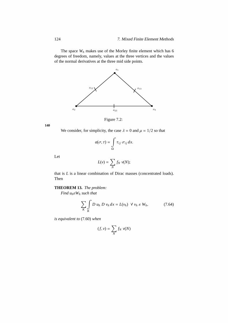
124 7. Mixed Finite Element Methods
The spaceWh makes use of the Morley finite element which has 6degrees of freedom, namely, values at the three vertices andthe valuesof the normal derivatives at the three mid side points.
Figure 7.2:140
We consider, for simplicity, the caseλ = 0 andµ = 1/2 so that
a(σ, τ) =∫
Ω
τi j σi j dx.
LetL(v) =
∑
N
fN v(N);
that isL is a linear combination of Dirac masses (concentrated loads).Then
THEOREM 13. The problem:Find uhεWh such that
∑
K
∫
K
D uh D vh dx= L(vh) ∀ vh ε Wh, (7.64)
is equivalent to(7.60)when
( f , v) =∑
N
fN v(N)

7.11. Equilibrium Elements for the Plate Problem 125
in the sense that
uh(N) =Wh(N) at the vertices N,
andσh|K = Duh|K , K ε Th.
Proof. Let uh be a solution of (7.64). 141
Define
σ∗h|K = Duh|K and w∗hεMh by w∗h(N) = uh(N).
We will show thatσ∗h(N),w∗h is the solution of (7.60). Sinceuh is asolution (7.64), we have
∑
K
∫
K
σ∗h Dvh dx= L(vh) ∀ vh ε Wh (7.65)
Using Green’s formula, we obtain
∑
K
∫
∂K
Mn(σ∗h)∂vh
∂n+
∫
∂K
Mns(σ∗h)∂vh
∂s
= L(vh) ∀ vh ε Wh (7.66)
If bi is one mid side point, then substitutingvh satisfying:
vh = 0 at the vertices
∂vh
∂n=
1 at bi
0 at the other nodesb j , j , i
in the above equation we obtain thatMn(σ∗h) is continuous atbi (by using7.59b). This proves that∗
hεVh.
Sinceσ∗hεVh, equation (7.66) gives
∑
K
∫
∂K
Mns(σ∗h)∂vh
∂s=
∑
N
fNvh(N) ∀ vh ε Wh
126 7. Mixed Finite Element Methods
But∑
K
∫
K
Mns(σ∗h)∂vh
∂s= −
∑
N
R(σ∗h, N) vh(N).
Hence 142∑
K
R(σ∗h,N) vh(N) = −∑
N
fN vh(N) ∀ vh ε Wh. (7.67)
Let vhεMh. Consider ˜vhεVh defined by
vh(N) = vh(N),∂
∂nvh(bi) = 0.
Then (7.67) gives∑
K
R(σ∗h,N) vh(N) = −∑
N
fN vh(N)
Therefore∑
N
R(σ∗h,N) vh(N) = −∑
N
fN vh(N) ∀ vh ε Mh.
This is nothing but the second equation in (7.60) withσh replaced byσ∗h. Now
a(σ∗h, τ) =∑
K
∫
K
(σ∗h)i j τi j
=
∑
K
∫
K
∂2uh
∂xi ∂x jτi j
=
∑
K
∫
K
Mn(τ)∂uh
∂n+
∫
K
Mns(τ)∂uh
∂s∀ τ ε Vh
by Green’s formula.The first term in the right side is zero sinceuhεWh andτεVh. The
second term equals−∑
NR(τ,N)uh(N). Hence we obtain
a(σ∗h, τ) +∑
N
R(τ,N) w∗h(N) = 0 ∀ τ ε Vh,
7.11. Equilibrium Elements for the Plate Problem 127
sinceuh(N) = w∗h(N).Thusσ∗h,w
∗h is a solution of (7.60). By uniqueness we haveσh =143
σ∗h andw∗h = wh.Thus we have proved that (7.64)⇒ (7.60). Letσh,wh be the solu-
tion of (7.60). We will show thatuh defined by
uh(N) = wh(N) for each vertex N (7.68)
Duh|K = σh|K for each K ε Th (7.69)
is the solution of (7.64).It is easy to see that (7.68) and (7.69) define a uniqueuh such that
uh|K ε P2(K) for eachKεTh. We will prove that thisuhεWh.From the first equation in (7.60), we obtain
∑
K
∫
∂K
Mn(τ)∂uh
∂n= 0 ∀ τ ε Vh.
This implies∂uh/∂n is continuous at mid side points and∂uh/∂n = 0at the boundary mid side points. HenceuhεWh.
Let vhεWh. Then there existsvhεMh such that ˜vh(N) = vh(N). Hencethe second equation in (7.60) gives
∑
R(σh, N) vh(N) = −∑
fN vh(N).
This shows∑
K
∫
K
Duh Dvh =
∑
N
fN vh.
This proves (7.60)⇒ (7.64).Thus the Hermann-Johnson method and the Morley nonconforming 144
method are equivalent, in this particular case where the load is a sum ofconcentrated loads.
Exercise 7.Let K be a triangle. LetPK = P2(K) and
∑
K
=
δai ,∂
∂nδai j , 1 ≤ i < j ≤ 3
,
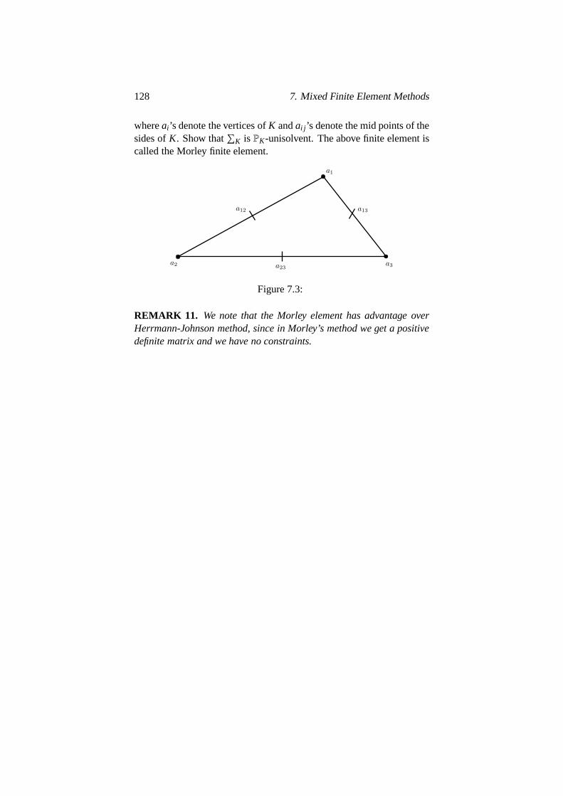
128 7. Mixed Finite Element Methods
whereai ’s denote the vertices ofK andai j ’s denote the mid points of thesides ofK. Show that
∑
K is PK-unisolvent. The above finite element iscalled the Morley finite element.
Figure 7.3:
REMARK 11. We note that the Morley element has advantage overHerrmann-Johnson method, since in Morley’s method we get a positivedefinite matrix and we have no constraints.

Chapter 8
Spectral Approximation forConforming Finite ElementMethod
8.1 The Eigen Value Problem
Let V andH be Hilbert spaces such thatV → H. We also assume that145
this imbedding is compact. Let‖· ‖1 denote the norm inV. The normin H is denoted by‖· ‖ or ‖· ‖0 and the scalar product inH is (· , · ). Weidentify H with its dualH′.
Let a(· , · ) : V × V → R be a continuous, symmetric bilinear formwhich isV-coercive withα as the coercive constant.
We shall consider the eigen value problem:FinduεV, µεR such that
a(u, v) = µ(u, v) ∀ v ε V (8.1)
In the following, for an operator⊤ : H → H, we write
‖ ⊤ ‖= SupfεH, f,0
‖ ⊤ f ‖‖ f ‖
.
129

130 8. Spectral Approximation for Conforming Finite...
8.2 The Operator⊤
The operator⊤ : H → V is defined as follows. IffεH then⊤ f isdefined to be the unique solution of the variational equation
a(⊤ f , v) = ( f , v) ∀ v ε V.
By Lax-Milgram Lemma⊤ f is well defined for all fεH. As theimbeddingV → H is compact we obtain that⊤, considered as an oper-146
ator fromH into H, is compact. The symmetry ofa(· , · ) implies that⊤is symmetric. It is easy to see that (8.1) is equivalent to:
Find uεV andλεR such that
⊤u = λu (8.2)
Theµ andλ in (8.1) and (8.2) have the relation
λµ = 1.
From the Spectral Theorem for compact self-adjoint operators wehave:
Sp(⊤) is a countable set with no accumulation point other than zero.Every point in Sp(⊤) other than zero is an eigenvalue of⊤ with finitemultiplicity.
8.3 Example
The model problem for (8.1) is
V = H1(Ω), H = L2(Ω)
whereΩ is a smooth bounded open subset ofRn,
a(u, v) =∫
Ω
∇u.∇v
The compactness of the imbeddingH1(Ω) → L2(Ω) is well known.Problem (8.1) corresponds to:
8.4. Approximate Problem 131
FinduεH1(Ω), µεR such that
−∆u = u in Ω,
u = 0 on ∂Ω(8.3)
We note that⊤ is the inverse of−∆. 147
8.4 Approximate Problem
Let Vh → V be a finite element subspace ofV. We consider the approx-imate eigen value problem:
Finduh ε Vh, µh ε R such that
a(uh, vh) = µh(uh, vh) ∀ vh ε Vh (8.4)
Here again, we introduce an operator⊤h : H → H where⊤h f is theunique solution of
a(⊤h f , vh) = ( f , vh) ∀ vh ε Vh. (8.5)
As in the continuous case, we have‖ ⊤h ‖≤ c/α which shows that⊤h is uniformly bounded. Again (8.4) is equivalent to:
FinduhεVh andλh = 1/µh such that
⊤h uh = λh uh (8.6)
It is obvious that⊤h is a self-adjoint, compact operator.We assume that
‖ ⊤ − ⊤h ‖≤ ε(h) (8.7)
and‖ (⊤ − ⊤h) f ‖≤ e(h) (8.8)
for all smoothf and⊤ f . Further, we assume 148
0 ≤ e(h) ≤ ε(h) and ε(h)→ 0 (8.9)

132 8. Spectral Approximation for Conforming Finite...
EXAMPLE. Let
Vh = vh ε H1(Ω) : vh|K ε Pk(K), K ε Th
whereTh is a regular family of triangulations ofΩ. We have (cf. Chapter5)
‖ ⊤ f − ⊤h f ‖0,Ω≤ chs+1 ‖ f ‖s−1,Ω, 1 ≤ s≤ k, (8.10)
provided thatΩ is a convex polygon and that
‖ ⊤ f ‖s+1≤ c ‖ f ‖s−1,Ω . (8.11)
From GRISVARD [22] this is atleast true fors = 1, which showsthatε(h) = ch2 ande(h) = 0(hk+1).
8.5 Convergence and Error Estimate for the EigenSpace.
Assumption (8.7) (8.9) show that⊤h→ ⊤ in norm.From KATO [26] (Chapter 5. Section 4.3) we know that the spec-
trum of ⊤h converges to the spectrum of⊤ in the following sense:For all non-zeroλεSp(⊤) with multiplicity m and for eachh such thatε(h) < d/2, where
d = minλ′εSp(⊤)
|λ − λ′|,
there exist exactlym eigen valuesλihεSp(⊤h) (counted according tomultiplicity) such that
|λ − λih| ≤ ε(h).
149
Let Γ = zεC : |z− λ| = d/2. We know that
P = −1
2πi
∫
Γ
Rz(⊤) dz, (8.12)
Ph = −1
2πi
∫
Γ
Rz(⊤h) dz, ε(h) < d/2, (8.13)

8.5. Convergence and Error Estimate for the Eigen Space. 133
whereRz(⊤) = (⊤ − z)−1, are the spectral projections on to the eigen-spacesE andEh associated withλ andλih’s. The dimension of each ofthe spacesE andEh is m (See KATO [26], Chapter 4, Section 4.3).
LEMMA 1. For uεE, we have
‖ u− Phu ‖≤ c2 ‖ (⊤ − ⊤h) u ‖ . (8.14)
Proof. We consider
Rz(⊤) − Rz(⊤h) = Rz(⊤h)(⊤h − z)Rz(⊤) − Rz(⊤h)(⊤ − z)Rz(⊤)
= Rz(⊤h)(⊤h − ⊤)Rz(⊤).
Hence
P− Ph = −1
2πi
∫
Γ
Rz(⊤h)(⊤h − ⊤)Rz(⊤) dz.
Let uεE. Then we have
Pu= u,⊤u = λu and Rz(⊤)u1
λ − zu.
Therefore 150
u− Phu = −1
2πi
∫
Γ
Rz(⊤h)λ − z
dz (⊤ − ⊤h) u.
We show that the integral on the right is bounded. Indeed, forzεΓandε(h) < d/2 we have
⊤h − z= ⊤h − ⊤ + ⊤ − z
= ((⊤h − ⊤) Rz(⊤) + I ) (⊤ − z),
which impliesRz(⊤h) = Rz(⊤) (I + Ah)−1,
whereAh = (⊤h − ⊤) Rz(⊤).

134 8. Spectral Approximation for Conforming Finite...
If P(⊤) denotes the resolvent set of⊤ then, asRz(⊤) is continuousin zεP(⊤) andΓ is a compact subset ofP(⊤), we obtain
‖ Rz(⊤) ‖≤ c1 for all z εΓ,
and‖ Ah ‖≤ c1ε(h), wherec1 is a constant. This implies
‖ (I + Ah)−1 ‖≤ 2 for ε(h) ≤1
2c1.
Thus‖ u− Phu ‖≤ c2 ‖ (⊤ − ⊤h) u ‖ .
LEMMA 2. If the eigen vectors in E are smooth enough, we have
δ(E, Eh) ≤ c e(h), (8.15)
where151
δ(E, Eh) = Supd(u,Eh) : u ε E, ‖ u ‖= 1.
Remark 1. In this chapter we follow closely OSBORN [34]. We willuse the result: “In a Hilbert spaceH, δ(E,Eh) = δ(Eh,E)”. Osborn,however, considers the more general case of a non-self-adjoint operatorin a Banach space, which involves more complicated arguments.
8.6 Error Estimates for the Eigen Values.
Let Qh = Ph|E, the restriction ofPh to E. ThenQh mapsE into Eh. Weprove thatQh is invertible for smallh.
Indeed, forh small enough we have dimE = dim Eh.Let fεE be such thatQh f = 0. Then
‖ f ‖=‖ f − Qh f ‖=‖ f − Ph f ‖≤ c2ε(h) ‖ f ‖,
where we have used Lemma 1. Therefore, forc2ε(h) < 1 we have‖ f ‖= 0. HenceQh is invertible forε(h) < min(d/2, 1/c2).
8.6. Error Estimates for the Eigen Values. 135
Let us evaluate‖ Q−1h ‖. If fεE with ‖ f ‖= 1, then
1− ‖ Qh f ‖≤‖ f − Ph f ‖≤ c2 ε(h).
Therefore‖ Qh f ‖≥ 1/2, if ε(h) ≤ 1/2c2
and 152
‖ Q−1h ‖≤ 2, for ε(h) ≤ 1/2c2.
Let ⊤h : E→ E be defined by
⊤h = Q−1h ⊤h Qh.
The eigenvalues of⊤h are againλih, i = 1, 2, . . . ,m (but the eigenvectorsof ⊤h are different from those of⊤h).
Let WjhεE, ‖ Wjh ‖= 1 be an eigen vector of⊤h associated with theeigen valueλ jh. Therefore,
λ − λ jh = ((λ − λ jh) w jh, w jh)
= ((⊤ − ⊤h) w jh, w jh)
≤ SupφεE,‖φ‖=1
((⊤ − ⊤h) φ, φ).
Now
⊤ − ⊤h = ⊤ − Q−1h ⊤h Qh = ⊤ − Q−1
h ⊤h Ph
= ⊤ − Q−1h Ph ⊤h.
Hence⊤ − ⊤h = Q−1
h Ph (⊤ − ⊤h), (8.16)
sincePh commutes with⊤h andQ−1h Phu = u for uεE. Hence
‖ (⊤ − ⊤h)φ ‖≤ 2 ‖ (⊤ − ⊤h)φ ‖ for all φεE
since‖ Q−1
h ‖≤ 2, ‖ Ph ‖≤ 1 for ε(h) ≤ 1/2c1.
Therefore 153
136 8. Spectral Approximation for Conforming Finite...
|λ − λ jh| ≤ 2e(h) for ε(h) ≤ min(1/2c1, d/2) (8.17)
Application. In the example given in Section 8.3, where⊤ is the inverseof the negative Laplace operator, we get
|λ − λih| ≤ chk+1, 1 ≤ i ≤ m, (8.18)
d(E,Eh) ≤ chk+1, (8.19)
sincee(h) ≤ chk+1 provided that the eigen functions inE are inHk+1
(This may happen even thoughΩ is a polygon: IfΩ =]0, 1[2 the eigenfunctions are known explicitly and they areC∞. In fact, the eigen func-tions are
unm = Sin nπx.Sin mπx.
However, the error estimate for|λ − λ jh| can be improved as will beshown in the following section. One indeed has
|λ − λ jh| ≤ ch2k .
8.7 Improvement of the Error Estimate for theEigen Values.
We denote bySh the projection onEh alongE⊥. We notice that
Rh = Q−1h Ph
is the projection onE alongE⊥h .

8.7. Improvement of the Error Estimate for the... 137
Figure 8.1:154
Sh andRh are related by
LEMMA 3. Sh = R∗h.
Proof. Foru, vεH, we have
(u,Shφ) = (Phu,Shφ), since PhSh = Sh and P∗h = Ph,
= (PhRhu,Shφ), since Rh is the projection onE alongE⊥h ;
= (Rhu,Shφ)
= (Rhu,PShφ), since PRh = Rh and P = P∗,
= (Rhu,Pφ), since PSh = P,
= (Rhu, φ).
We will now prove a Lemma which will give an upper bound for‖ P− Sh ‖.
LEMMA 4. We have
‖ P− Sh ‖≤δ(Eh,E)
1− δ(Eh,E)(8.20)
155
138 8. Spectral Approximation for Conforming Finite...
Proof. SinceSh is the projection onEh alongE⊥ we haveP = PSh. IfxεEh and‖ x ‖= 1 then
‖ x− Px ‖= d(x,E) ≤ SupxεEh,‖x‖=1
d(x,E) = δ(Eh,E).
Therefore,
‖ y− Py ‖≤ δ(Eh,E) ‖ y ‖ for all y εEh (8.21)
Now, for anyxεH,
‖ Shx ‖ ≤‖ Shx− PShx ‖ + ‖ PShx ‖≤ δ(Eh,E) ‖ Shx ‖ + ‖ Px ‖ .
Thus
‖ Shx ‖≤1
1− δ(Eh,E)‖ x ‖ (8.22)
Hence we obtain
‖ (P− Sh)x ‖ =‖ PShx− Shx ‖≤ δ(Eh,E) ‖ Shx ‖, by (8.21),
≤ δ(Eh,E)1− δ(Eh,E)
‖ x ‖, using (8.22)
Therefore
‖ P− Sh ‖≤δ(Eh,E)
1− δ(Eh,E).
Finally we have from (8.16),
((⊤ − ⊤h) φ, φ) = (Rh (⊤ − ⊤h)φ, φ)
= ((⊤ − ⊤h) φ, Shφ)
= ((⊤ − ⊤h)φ, φ) + ((⊤ − ⊤h)φ,Shφ − φ),
whereφεE and‖ φ ‖= 1.156
8.7. Improvement of the Error Estimate for the... 139
ForφεE, using Lemma 4 and Lemma 2, we obtain
‖ φ − Sh ‖≤δ(Eh,E)
1− δ(Eh,E)≤ k e(h),
for sufficiently smallh, wherek is a constant.We know that for allφεE with ‖ φ ‖= 1
λ − λih = ((⊤ − ⊤h) φ, φ).
Hence|λ − λih| ≤ Sup
φεE,‖φ‖=1((⊤ − ⊤h)φ, φ) + k(e(h))2.
Thus we have proved
THEOREM 5. When E is a smooth subset of H and h is sufficientlysmall we have
|λ − λih| ≤ SupφεE,‖φ‖=1
((⊤ − ⊤h)φ, φ) + k(e(h))2, (8.23)
where k is a constant.
Application. In the case of the example in Section 8.3, we give an157
estimate ofαh = Sup
φεE,‖φ‖=1((⊤ − ⊤h)φ, φ).
Let w be the solution of
a(v,w) = (φ, v) ∀ v ε V, (8.24)
whereφεE and‖ φ ‖= 1.We have
((⊤ − ⊤h)φ, φ) = a((⊤ − ⊤h)φ, w)
= a((⊤ − ⊤h)φ,w− vh) for all vh ε Vh,
sincea((⊤ − ⊤h)φ, vh) = 0 for all vh ε Vh.
140 8. Spectral Approximation for Conforming Finite...
If wεHk+1(Ω), we get
‖ w− vh ‖1≤ chk ‖ w ‖k+1≤ chk ‖ φ ‖k−1,
using regularity theorem and the error estimates in Chapter5.SinceE is finite-dimensional there exists a constantc such that
‖ φ ‖k−1≤ c ‖ φ ‖= c.
Finally, we have
αh ≤ chk ‖ (⊤ − ⊤h)φ ‖1≤ ch2k,
provided thatE ⊂ Hk+1.158
Thus we have proved
THEOREM 6. For the model problem (See Section 8.3) we have
|λ − λih| ≤ ch2k,
provided E⊂ Hk+1(Ω), the solution of(8.24) is in Hk+1(Ω) and h issmall.
REMARK 2. Error estimates for the semi-discrete approximation toparabolic equation of the form
(
dudt, v
)
+ a(u, v) = ( f , v) for all v ε V,
u(0) = v, v ε V,
can be obtained using spectral approximation. The reader isreferred toTHOMEE [44], [45].
Chapter 9
Nonlinear Problems
Introduction.
We consider here problems of the following type: 159
FinduεC such that
J(u) ≤ J(v) for all v ε V, (9.1)
whereC is a closed, convex subset of a Banach spaceV andJ : V → Ris a convex, lower semi-continuous (l.s.c.) function.
We denote by (· , · ) the duality pairingV′−V and‖· ‖ the norm inV.We write (9.1) in the form:
FinduεC such thatJ(u) = Inf
vεCJ(v). (9.2)
The existence and uniqueness of the solutions of (9.2) is given by
THEOREM 1. Assume that J is coercive on C, that is
J(v)→ ∞ if ‖ v ‖→ ∞, v ε C. (9.3)
Then problem(9.2)has atleast one solution provided that V is reflexive.If J is strictly convex, then(9.2)has almost one solution.
The proof of theorem 1 can be found in EMELAND-TEMAN [15].
141
142 9. Nonlinear Problems
Exercise 1.If J is Gateaux-differentiable, thenu is a solution of (9.2) 160
iff
(J′(u), v− u) ≥ 0 for all v ε C.
If C is affine linear, (9.1) implies
(J′(u), v− u) = 0 ∀ v ε C.
Approximation.Let Vh be a finite-dimensional subspace ofV andCh a closed, con-
vex subset ofVh. Then the approximate problem corresponding to (9.2)is:
Find uh ε Ch such that
J(uh) = InfvhεCh
J(vh). (9.4)
We assume thatJ is strictly convex and coercive. Moreover, weassume thatCh approximatesC.
For all v ε C there exists vh ε Ch
such that vh→ v (strongly) as h→ 0;
(9.5)
If wh w ε V as h→ 0 and wh ε Ch
then w ε C.
(9.6)
Then one can easily prove that the solutionuh of (9.4) converges weaklyto u, the solution of (9.2).
Note that (9.5) implies thatCh has to be sufficiently big and (9.6)demandsCh to be sufficiently small.
To get strong convergence ofuh to u, one needs some strong mono-161
tonicity; there existsα, γ > 0 such that
(J′(u) − J′(v), u− v) ≥ α ‖ u− v ‖γ,∀u, v ε C (9.7)
143
Case 1.We obtain an error estimate when Ch = C∩ Vh. From Exercise1, we have
(J′(u), v− u) ≥ 0 ∀ v ε C, (9.8)
(J′(uh), vh − uh) ≥ 0 ∀ vh ε Ch. (9.9)
As Ch = C∩Vh, choosing v= uh in (9.8)and adding to(9.9), we get
(J′(u) − J′(uh), uh − u) + (J′(uh), vh − u) ≥ 0.
Therefore (assuming J to be continuously differentiable)
α ‖ uh − u ‖γ≤ (J′(uh), vh − u) ≤ c ‖ vh − u ‖,
since uh is bounded. Finally,
‖ uh − u ‖≤ c InfvhεCh
‖ vh − u ‖1/γ, (9.10)
provided J′ is weakly continuous.Note that
InfvhεCh
‖ vh − u ‖
measures how good is the approximation Ch to C. Note also that, as uh
is bounded, it is enough if(9.7)holds on bounded subsets of C.
Exercise 2.Let φ : V → R be Lipschitz but not differentiable. Then 162
J(u) = InfvεC
[J(v) + φ(v)]
is equivalent to
(J′(u), v− u) + φ(v) − φ(u) ≥ 0 ∀ v ε C.
Derive an error estimate similar to (9.10).
Case 2.When C is of the form
C = v ε V : b(v, µ) = (φ, µ) ∀ µ ε M, (9.11)
144 9. Nonlinear Problems
where M is a Hilbert space, b(· , · ) is a continuous, bilinear form onV × M andφεM satisfying Brezzi’s condition (See Chapter 7), Problem(9.1) is equivalent to:
Find u, λ ε V × M such that
< J′(u), v > +b(v, λ) = 0 ∀ v ε V, (9.12)
b(u, µ) = (φ, µ) ∀ µ ε M. (9.13)
We notice that(9.11) is affine linear and from Exercise 1 we obtainthat (9.1) is equivalent to
(J′(u), v− u) = 0 ∀ v ε C. (9.14)
Let B : V → M be defined by
(Bv, µ) = b(v, µ) ∀ v ε V, µ ε M.
Clearly C= v+ KerB, where vεC. This together with(9.14)implies163
J′(u) ε (KerB)⊥ = Im B∗,
which is closed from Brezzi’s condition. Hence there existsλεM suchthat
J′(u) = −B∗λ.
Thus(J′(u), v) + b(v, λ) = 0 ∀ v ε V.
uεC implies b(u, µ) = (φ, µ)∀µεM.So we have proved that(9.1) implies(9.12)and (9.13).If (9.12)and (9.13)hold, then uεC and
(J′(u), u) = −b(u, λ) = −b(v, λ) ∀ v ε C
Hence〈J′(u), v− u〉 = 0 ∀vεC, which is equivalent to(9.1).Thus we proved the equivalence of(9.1)and (9.12) (9.13).A natural approximation Ch to C will be
Ch = v ε V : b(v, µh) = (φ, µh) ∀ µh ε Mh,
where Mh approximates M. In this case
Ch 1 C.

145
EXAMPLE 1. Nonlinear Dirichlet Problem.164
V =W1,p(Ω),C = V
J(v) =1p
∫
Ω
|∇v|p dx−∫
Ω
f v dx,
wheref ε Lq, 1/p+ 1/q = 1
For 1< p < ∞,W1.p(Ω) is reflexive andJ(v) → ∞ as‖ v ‖→ ∞. Onehas
(J′(u), v) =∫
Ω
|∇u|p−2∇u.∇v dx−∫
Ω
f v dx,
and some strong monotonicity results of the type (9.7) are proved inGLOWINSKI-MARROCCO [19].
EXAMPLE 2. The Obstacle Problem.
V = H1(Ω),
C = v ε H1(Ω) : v ≥ 0 a. e. on Ω,
J(v) =12
∫
Ω
|∇v|2 dx−∫
Ω
f v dx.
Existence and uniqueness of the solution of the minimization prob-lem are straightforward.
Let Vh be the standard Lagrange finite element space of degree 1andCh = C∩Vh. One has (9.10) withγ = 2; therefore it seems that onegets
‖ u− uh ‖= 0(√
h)
since the interpolateπhuεCh as long asuεC. However, one has 165
(J′(uh), vh − u) = (J′(u), vh − u) + (J′(uh) − J′(u), vh − u)
≤ (−∆u− f , vh − u) +Mε
2‖ uh − u ‖21 +
M2ε‖ vh − u ‖21 .

146 9. Nonlinear Problems
Hence‖ u− uh ‖21≤ c
(
‖ vh − u ‖20 + ‖ vh − u ‖21)
Therefore‖ u− uh ‖1= 0(h).
EXAMPLE 3. Elasto - Plastic Torsion.J andV as is Example 2,
C = v ε H1(Ω) : |∇v| ≤ 1 a. e. on Ω,
Vh same as in Example 2 andCh = C ∩ Vh.In this case the interpolateπhu is not inCh whereasu is in C. One
gets 0(h1/2−ε).
EXAMPLE 4. The Flow of a Bingham Fluid in a Cylindrical Pipe. Thisis a particular case of Exercise 2 withJ,V as above and
φ(v) =∫
Ω
|∇v|dx.
9.2 Generalization
Note thatJ′ : V → V′ satisfies
(J′(u) − J′(v), u− v) ≥ 0 ∀ u, v ε V.
166
An operatorA : V → V′ is said to bemonotoneif
(Au− Av, u− v) ≥ 0 ∀ u, v ε V. (9.15)
A is boundedif A maps bounded sets ofV into bounded sets ofV′.A is hemi-continuousif
limλ→0
(A(u+ λw), v) = (A(u), v) ∀ u, v,w ε V. (9.16)
A is coerciveif
(A(v), v)‖ v ‖
→ ∞ if ‖ v ‖→ ∞ for v ε C. (9.17)
We have

9.3. Contractive Operators. 147
THEOREM 2. If A is a monotone, bounded hemi continuous and co-ercive operator then the problem:
Find uεC such that
(A(u), v− u) ≥ 0 ∀ v ε C (9.18)
has atleast one solution.
For a proof of this Theorem see LIONS [28]. The problem (9.18)hasat most one solution ifA is strongly monotone, i.e. there existsα, γ > 0such that
α ‖ u− v ‖γ≤ (A(u) − A(v), u− v) ∀ u, v ε C (9.19)
The error analysis can be carried out in the same way.
9.3 Contractive Operators.
Let T : C → C be a mapping, whereC is a closed, convex subset of a167
Hilbert spaceH. The scalar product inH is denoted by (· , · ).We callT contractiveiff
‖ T x− Ty ‖≤‖ x− y ‖, ∀ x, y ε C. (9.20)
T is strictly contractiveiff there exists aθ with 0 < θ < 1 such that
‖ T x− Ty ‖≤ θ ‖ x− y ‖ ∀ x, y ε C. (9.21)
We say thatT is firmly contractiveiff (cf. BROWDER-PETRYSHN [8])
‖ T x− Ty ‖2≤ (T x− Ty, x− y) ∀ x, y ε C (9.22)
T is quasi firmly contractiveiff there exists aθ, 0 < θ < 1 such that
‖ T x− Ty ‖2≤ θ(T x− Ty, x− y) + (1− θ) ‖ x− y ‖2 (9.23)
Note that (9.22)⇒ (9.23)⇒ (9.20) and (9.21)⇒ (9.20).
Geometrical Interpretation of the Above Definitions Let yεC be afixed point ofT, i.e. Ty= y. If T is contractive andxεC thenT x lies in
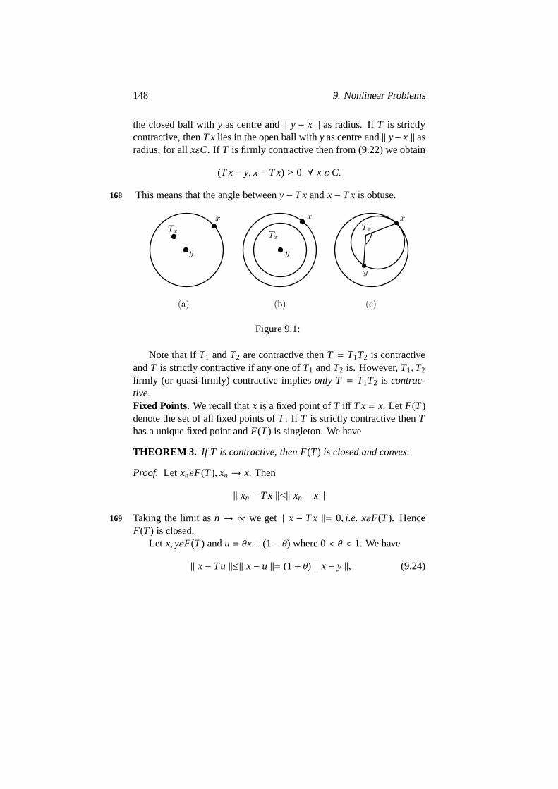
148 9. Nonlinear Problems
the closed ball withy as centre and‖ y − x ‖ as radius. IfT is strictlycontractive, thenT x lies in the open ball withy as centre and‖ y− x ‖ asradius, for allxεC. If T is firmly contractive then from (9.22) we obtain
(T x− y, x− T x) ≥ 0 ∀ x ε C.
This means that the angle betweeny− T xandx− T x is obtuse.168
(a) (b) (c)
Figure 9.1:
Note that ifT1 andT2 are contractive thenT = T1T2 is contractiveandT is strictly contractive if any one ofT1 andT2 is. However,T1,T2
firmly (or quasi-firmly) contractive impliesonly T = T1T2 is contrac-tive.Fixed Points.We recall thatx is a fixed point ofT iff T x= x. Let F(T)denote the set of all fixed points ofT. If T is strictly contractive thenThas a unique fixed point andF(T) is singleton. We have
THEOREM 3. If T is contractive, then F(T) is closed and convex.
Proof. Let xnεF(T), xn→ x. Then
‖ xn − T x ‖≤‖ xn − x ‖
Taking the limit asn → ∞ we get‖ x − T x ‖= 0, i.e. xεF(T). Hence169
F(T) is closed.Let x, yεF(T) andu = θx+ (1− θ) where 0< θ < 1. We have
‖ x− Tu ‖≤‖ x− u ‖= (1− θ) ‖ x− y ‖, (9.24)

9.3. Contractive Operators. 149
‖ y− Tu ‖≤‖ y− u ‖= θ ‖ x− y ‖, (9.25)
‖ x− y ‖≤‖ x− Tu ‖ + ‖ y− Tu ‖≤‖ x− y ‖, (9.26)
SinceH is strictly convex, we obtain using (9.24) and (9.25),
x− Tu= c(y− Tu) (9.27)
‖ x− Tu ‖2= c(y− Tu, x− Tu), (9.28)
‖ x− y ‖2=‖ x− Tu ‖2 + ‖ y− Tu ‖2 +2 ‖ x− Tu ‖ ‖ y− Tu ‖,
by (9.26),
‖ x− y ‖2 =‖ x− Tu+ Tu− y ‖2
=‖ x− Tu ‖2 + ‖ Tu− y ‖2 +2(x− Tu,Tu− y)
So(x− Tu,Tu− y) =‖ x− Tu ‖ ‖ y− Tu ‖> 0. (9.29)
From (9.28) and (9.29) we obtainc < 0.Equations (9.26) and (9.27) imply
‖ y− Tu ‖= 11+ |c|
‖ x− y ‖ .
This with (9.25) gives|c| ≥ (1 − θ)θ−1. Similarly using (9.24), (9.26)and (9.27) we obtain|c| ≤ (1− θ)θ−1. Thus
|c| = (1− θ) θ−1.
Hence 170
θ(x− Tu) = −(1− θ)(y− Tu).
ThereforeTu= θx+ (1− θ)y = u,
that isu ε F(T).
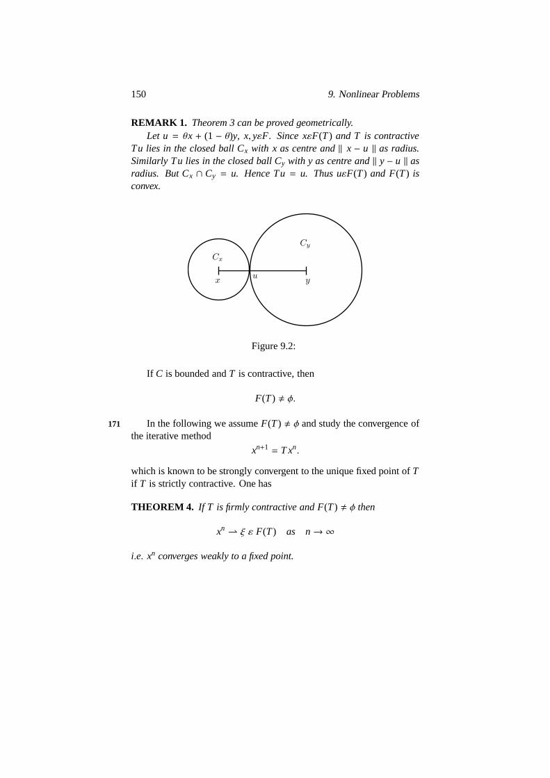
150 9. Nonlinear Problems
REMARK 1. Theorem 3 can be proved geometrically.Let u = θx + (1 − θ)y, x, yεF. Since xεF(T) and T is contractive
Tu lies in the closed ball Cx with x as centre and‖ x − u ‖ as radius.Similarly Tu lies in the closed ball Cy with y as centre and‖ y− u ‖ asradius. But Cx ∩ Cy = u. Hence Tu= u. Thus uεF(T) and F(T) isconvex.
Figure 9.2:
If C is bounded andT is contractive, then
F(T) , φ.
In the following we assumeF(T) , φ and study the convergence of171
the iterative method
xn+1= T xn.
which is known to be strongly convergent to the unique fixed point of Tif T is strictly contractive. One has
THEOREM 4. If T is firmly contractive and F(T) , φ then
xn ξ ε F(T) as n→ ∞
i.e. xn converges weakly to a fixed point.

9.3. Contractive Operators. 151
Proof. Let yεF(T). We have
‖ xn+1 − y ‖2≤ (xn+1 − y, xn − y)
But
12‖ xn+1 − xn ‖2 = 1
2‖ xn+1 − y ‖2 +1
2‖ xn − y ‖2 −(xn+1 − y, xn − y)
≤12‖ xn − y ‖2 −
12‖ xn+1 − y ‖2 .
Therefore
‖ xn+1 − y ‖2 + ‖ xn+1 − xn ‖2≤‖ xn − y ‖2,
‖ xN+1 − y ‖2 +N
∑
n=0
‖ xn+1 − xn ‖2≤‖ x − y ‖2,
which proves that‖ xn+1− xn ‖→ 0 andxn is a bounded sequence. Letxn′ x be a weakly convergent subsequence.
Since 172
(T x− Ty, T x− Ty+ y− x) ≤ 0
choosingy = xn′−1 we obtain(
T x− xn′ , T x− xn′+ xn′−1 − x
)
≤ 0
As n′ → ∞, we get(T x− x, T x− x) ≤ 0,
and hencexεF(T).As ‖ xn − y ‖2 is a decreasing sequence for anyyεF(T) it converges
to some numberP(y), and we conclude from the following Lemma thatthe whole sequencexn converges.
OPAL’S LEMMA 5. Let F ⊂ H be a subset of a Hilbert space H andxn a sequence such that
(i) ‖ xn − y ‖2→ P(y) as n→ ∞ for any yεF
152 9. Nonlinear Problems
(ii) any weakly converging subsequence xn′ z is such that z belongsactually to F.
Then xn ξεF.
Proof. Let xm′ y, xn′ zbe two converging subsequences, we have
‖ xn − y ‖2 =‖ xn − z+ z− y ‖2
=‖ xn − z ‖2 +2(xn − z, z− y)+ ‖ z− y ‖2
hence taking the limit followingm
P(y) = P(z) + 2(y− z, z− y)+ ‖ z− y ‖2= P(z)− ‖ z− y ‖2
and taking the limit followingn′173
P(y) = P(z) + 0+ ‖ z− y ‖2
hence‖ z− y ‖2= 0⇒ z= y.
Exercise 3.Prove Theorem 4 whenT is quasi firmly contractive.
THEOREM 6. Let T = QS where S is quasi-firmly contractive and Qis firmly contractive. Then
xn x ε F(T),
provided that F(T) is non-empty.
Proof. Let yεF(T). We have
‖ S xn − S y‖2≤ θ(S xn − S y, xn − y) + (1− θ) ‖ xn − y ‖2,
(S xn − S y, xn − y) =12‖ S xn − S y‖2 +1
2‖ xn − y ‖2
−12‖ S xn − S y+ y− xn ‖2 .
Therefore,
(1− θ2
) ‖ S xn−S y‖2 + θ2‖ S xn−S y+y−xn ‖2≤ (1− θ
2) ‖ xn−y ‖2 (9.30)
9.3. Contractive Operators. 153
In the same way,
‖ QS xn − y ‖2≤ (QS xn − y, S xn − S y)
=12‖ QS xn − y ‖2 +1
2‖ S xn − S y‖2
− 12‖ QS xn − y+ S y− S xn ‖2,
i.e. 174
12‖ xn+1 − y ‖2 +1
2‖ xn+1 − y+ S y− S xn ‖2≤ 1
2‖ S xn − S y‖2 (9.31)
From (9.30) and (9.31) we obtain
‖ xn+1−y ‖2 + ‖ xn+1−y+S y−S xn ‖2 +α ‖ S xn−S y+y−xn ‖2≤‖ xn−y ‖2
where
α =θ
2− θThis implies
‖ xN+1 − y ‖2 +N
∑
n=0
(
‖ xn+1 − y+ S y− S xn ‖2 +
+α ‖ S xn − S y+ y− xn ‖2)
≤‖ x − y ‖2 .
Therefore,
xn+1 − S xn→ y− S y,
S xn − xn→ S y− y,
xn+1 − xn→ 0.
Let xn′ x, T being contractive, we have
‖ T xn′ − T x ‖2≤‖ xn′ − x ‖2
that is(
xn′+1 − xn′+ x− T x, xn′+1
+ xn′ − T x− x)
≤ 0

154 9. Nonlinear Problems
and to the limit
(x− T x, x+ x− T x− x) ≤ 0
x = T x.
Once again we apply Opial’s Lemma to get the convergence of the175
whole sequencexn to a fixed point ofT.
Exercise 4.Let C ⊂ V be a closed convex subset of a Hilbert spaceV,then show that the projection mapPc : V → C is firmly contractive.
9.4 Application to Unconstrained Problem
We shall apply the previous results to the solution of
A(u) = 0.
whereA is a monotone operator fromD(A) into H; i.e.
(Au− Av, u− v) ≥ 0 ∀ u, v ε D(A).
A is said to bemaximal monotoneif E ⊂ H × H, GraphA ⊂ E,
(x1 − x2, y1 − y2) ≥ 0 ∀xi , yi ε E, i = 1, 2
impliesGraph A = E.
It is proved inBREZIS [4] that
THEOREM 7. A maximal monotoneiff
R(I + λA) = H for λ ≥ 0.
EXAMPLE 5. Let A : V → V′ satisfy (9.15) - (9.17) with176
V → Hdense
→ V′
Then the restriction ofA to
D(A) = v ε V : Av ε H
is a maximal monotone operator.

9.4. Application to Unconstrained Problem 155
Exercise 5.Use Theorem 6 to prove that the operator defined in Exam-ple 5 is monotone.
We have
LEMMA 8. If A is maximal monotone then
T = (I + λA)−1
is firmly contractive.
Proof. Let(I + λA)x = (I + λA)y.
Thenλ(A(x) − A(y)) = −(x− y)
Therefore− ‖ x− y ‖2= λ(A(x) − A(y), x− y) ≥ 0.
Hencex = y. This proves (I + λA) is one-one.From Theorem 6, we obtainR(I + λA) = H. Hence (I + λA)−1 is 177
well defined onH.Let
ui = T xi , xi ε H, i = 1, 2.
Thenui + λAui = xi .
We have to prove that
‖ T x1 − T x2 ‖2≤ (T x1 − T x2, x1 − x2),
i.e.(T x1 − T x2,T x1 − T x2 + x2 − x1) ≤ 0,
i.e.(u1 − u2, (u1 − u2) − (u1 − u2) − λ(Au1 − Au2)) ≤ 0,
i.e.−λ(u1 − u2,Au1 − Au2) ≤ 0,
which is true sinceA is monotone.
156 9. Nonlinear Problems
COROLLARY 1. The algorithm
xn+1= (I + λA)−1 xn (9.34)
converges weakly to a solution of
A(u) = 0 (9.35)
Note that algorithm(9.34)can be written as
xn+1 − xn
λ+ A(xn+1) = 0 (9.36)
and corresponds to an implicit scheme for178
∂u∂t+ A(u) = 0. (9.37)
Proof. SinceT = (I +λA)−1 is firmly contractive, algorithm (9.34) con-verges weakly to a fixed point ofT which is a solution of (9.35).
REMARK 2. Algorithm (9.34) is called aproximal point algorithm.Note that computing xn+1 at each step might be as difficult as the origi-nal problem except in some special cases.
REMARK 3. If A : V → V′ where V is a Hilbert space, then it is betterto choose H= V. Let J : V′ → V be the Riesz isometry. Then one hasto replace A by JA. Then algorithm(9.34)is an implicit scheme for
∂u∂t+ JA(u) = 0.
9.5 Application to Problems with Constraint.
We want to solve the problem
(A(u), v− u) ≥ 0 ∀ v ε C. (9.38)
If u is a solution of (9.38) then for anyλ > 0 we have
(u− λA(u) − u, v− u) ≤ 0 ∀ v ε C
9.5. Application to Problems with Constraint. 157
which impliesu = PCS u, where179
S u= u− λA(u).
Conversely ifu is a fixed point ofPCS, thenu is a solution of (9.38).We like to solve (9.38) via the algorithm
xn+1= PCS xn = PC(xn − λA(xn)). (9.39)
Note that ifJ is a convex,l.s.c., Gateaux differentiable function andA = J′ then (9.38) is the gradient algorithm with projection for solving
InfvεC
J(v).
We will now give some conditions onA andλ which will ensure theconvergence of the algorithm (9.39) to a solution of (9.38).
THEOREM 9. If A is strongly monotone, i.e.
(A(u) − A(v), u− v) ≥ α ‖ u− v ‖2 ∀ u, v ε C (9.40)
and Lipshitzian,
‖ A(u) − A(v) ‖≤ c ‖ u− v ‖ ∀ u, v ε C (9.41)
then the algorithm(9.39) converges strongly to the solution(9.38) forall 0 < λ < 2α/c.
Proof. S is strictly contractive for 0< λ < 2α/c. Indeed 180
‖ S u− S v‖2=‖ u− v ‖2 −2λ(A(u) − A(v), u− v)+
+λ2 ‖ A(u) − A(v) ‖2≤‖ u− v ‖2 (1− 2λα + λ2c2)
by (9.40) and (9.41) and
1− 2αλ + λ2c2 < 1 for 0< λ <2α
c2
From exercise 4, we know thatPC is firmly contractive. ThereforePCS is strictly contractive for 0< λ < 2α/c2. Thus the algorithm (9.39)converges strongly to the solution of (9.38).

158 9. Nonlinear Problems
We will now give a condition onA which will imply weak conver-gence of the algorithm (9.39).
THEOREM 10. If A−1 is coercive, namely
(A(u) − A(v), u− v) ≥ α ‖ A(u) − A(v) ‖2 ∀ u, v ε C (9.42)
then for0 < λ < 2α the algorithm(9.39)converges weakly to a solutionof (9.38).
Proof. We claim thatS is quasi firmly contractive forα < λ < 2α. Infact,
‖ S u− S v‖2 ≤‖ u− v ‖2 +(
λ2
α− 2λ
)
(A(u) − A(v), u− v) by (9.42)
= (1− θ) ‖ u− v ‖2 +θ(S u− S v, u− v)(9.43)
where181
θ = 2− λ/α.
Whenα < λ < 2α, we have 0< θ < 1.When 0< λ < α we obtainS to be firmly contractive. To prove
this use (9.43), the Schwarz inequality and the fact thatθε[1, 2] when0 < λ < α. ThusS is quasi firmly contractive for 0< λ < 2α. UsingTheorem 5, we obtain the conclusion of the Theorem.
REMARK 4. When A satisfies(9.42)and0 < λ < 2α, we obtain fromthe proof of Theorem 5 that
λA(xn) = xn − S xn→ x− S x= λA(x),
i.e. A(xn)→ A(x), (Strong convergence)whereas
xn→ x. (Weak convergence)
We also notice that x−S x is unique and therefore A(x) (x, the solu-tion of (9.38), need not be unique).

9.5. Application to Problems with Constraint. 159
EXAMPLE 6. Letf : H → R be convex,l.s.c. differentiable andA : V → H be a linear operator.We want to solve
InfvεV
f (Av). (9.44)
Note that (9.44) is equivalent to 182
InfyεC
f (y), (9.45)
whereC = R(A), the range ofA.Now apply the algorithm (9.39). The projection onC is easy to
compute. In fact,PC = A(A∗A)−1 A∗.
The nonlinear Dirichlet problem and the Minimal surface problemare particular cases of the abstract problem.
EXAMPLE 7. Let us consider
∂u∂t+ Au= 0,
u(0) = u,(9.46)
which has a solution providedA is maximal monotone.We like to solve this problem via the algorithm
un+1= F(λ) un. (9.47)
In BREZIS [4] one can find the proof of
THEOREM 11. If F (λ) is a contraction and if
limλ→0
x− F(λ)xλ
= A(x) exists, (9.48)
then 183
(F(t/n))n u → u(t) uniformly.
160 9. Nonlinear Problems
Applications:
1. If F(λ) = I − λA, whereA satisfies (9.40), thenF(λ) is a con-traction for 0< λ < 2α. The limit in (9.48) exists and hence thealgorithm (9.47) converges.
2. Let F(λ) = (I + λA)−1, whereA is maximal monotone. Thenby Lemma 7,F(λ) is firmly contractive and hence contractive.Existence of the limit (9.48) is proved inBREZIS [4] In this casealso algorithm (9.47) converges.
REMARK 5. Theorem 11 can be used to prove that F(λ) = PC(I −λA)gives a sequence converging to the solution of
(
dudt+ Au, v− u
)
≥ 0 ∀ v ε C,
u(0) = u.
REMARK 6. If A is linear, monotone and closed then A is maximalmonotone.
EXAMPLE 8. The Flow of a Bingham Fluid: Consider the problem:Findσε(L2(Ω)), uεH1
(Ω) such that
J′(σ) − ∇u = 0 (9.49)
(σ,∇v) = ( f , v) ∀ v ε H1(Ω),
where184
J(σ) =12‖ σ − PKσ ‖2 (L2(Ω))n,
K = σ ε (L2(Ω))n : |σ(x)| ≤ 1 a. e. in Ω.
It is possible to prove that (9.49) is equivalent to the Bingham flowgiven in Example 4. It can be proved that
J′(σ) = σ − PKσ.
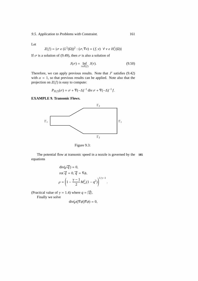
9.5. Application to Problems with Constraint. 161
LetZ( f ) = σ ε (L2(Ω))2 : (σ,∇v) = ( f , v) ∀ v ε H1
(Ω)
If σ is a solution of (9.49), thenσ is also a solution of
J(σ) = InfτεZ( f )
J(τ). (9.50)
Therefore, we can apply previous results. Note thatJ′ satisfies (9.42)with α = 1, so that previous results can be applied. Note also that theprojection onZ( f ) is easy to compute:
PZ( f )(σ) = σ + ∇(−∆)−1 divσ + ∇(−∆)−1 f .
EXAMPLE 9. Transonic Flows.
Figure 9.3:
The potential flow at transonic speed in a nozzle is governed by the 185
equations
div(ρ−→q ) = 0,
rot−→q = 0,−→q = ∇φ,
ρ =
(
1−γ − 1
2M2∞(1− q2)
)1/γ−1
.
(Practical value ofγ = 1.4) whereq = |−→q |.Finally we solve
div(ρ(|∇φ|)∇φ) = 0,
162 9. Nonlinear Problems
φ|Γ1 = φ,
∂φ
∂n|Γ2 = 0
Let M = q/a, wherea = ργ−1
M2∞
. M is called theMach number.The equation is elliptic forM < 1 and hyperbolic forM > 1.WhenM < 1 continuous piecewise linear finite element can be used.
For M > 1, we do not know much (see COURANT- FRIEDRICHS[13]).
The reader can refer to GLOWINSKI-PIRONNEAU [20],[21],RAVIART [36], CIAVALDINI-POGU-TOURNEMINE [12],J. ROUX [40].

Bibliography
[1] ADAMS, R.A.: Sobolev Spaces, Academic Press, 1976. 186
[2] AMARA, M. and J.M. THOMAS:Une methode d’elements finisequilibre pour le probleme de l’elasticite lineaire, C.R. Acad. Sci.Paris, Serie A, Seance du 3 Avril 1978.
[3] BERCOVIER, M. and O. PIRONNEAU:Estimations d’erreurpour la resolution du probleme de STokes en elements finis con-formes de Lagrange, C.R. Acad. Sci. Paris, t 285 Serie A (1977),557 – 559.
[4] BREZIS, H.: Operateurs Maximaux Monotones, Lecture Notes #5, North Holland, 1975, RAIRO, 1974.
[5] BREZZI, F.: On the existence, Uniqueness and Approximationof Saddle point problems arising from lagrangian multipliers,RAIRO, Vol. 8, 1974, 129 – 151.
[6] BREZZI, F.; J. RAPPAZ and P.A. RAVIART:Finite element ap-proximation of bifurcation problem (to appear).
[7] BREZZI, F. and P.A. RAVIART:Mixed finite element methods for4th order elliptic equations, Topics in Numerical Analysis III, ed.by John, J.H. Miller, Academic Press, 33 – 57.
[8] BROWDER, F.E. and W.V. PETRYSHN:Construction of fixedpoints of nonlinear mappings in Hilbert Spaces, J. Math. Anal.Appl., 20 (1977), 197 – 228.
163

164 BIBLIOGRAPHY
[9] CIARLET, P.G.:The Finite Element Method for elliptic problems,187
North Holland, 1978.
[10] CIARLET, P.G. and P.A. RAVIART:A Finite Element Method forthe Biharmonic Equation, Mathematical Aspects of Finite Ele-ments in Partial Differential Equations, by Carl de Boor, AcademicPress, 1974, 125 – 146.
[11] CIAVALDINI, J.F. and J.C. NEDELEC:Sur l’element de Fraeijsde Veubeke et Sander, Serie Analyse Numerique, RAIRO, 1974,29 – 46.
[12] CIAVALDINI, J.F.: M.POGU and G. TOURMINE:Une nouvelleapproche daus le plan physique pour le calcul d’elements sub-critiques et Stationnaires autour d’un profil portant, Journal demecanique, 16 (1977) 257 – 288.
[13] COURANT, R and K.O. FRIEDRICHS:Supersonic flow andShock Waves, J. Wiley, 1948.
[14] CROUZEIX, M. and P.A. RAVIART:Conforming and Noncon-forming Finite Elements Methods for solving the StationaryStokesEquations, RAIRO, 1974, 1 – 53.
[15] EKELAND, I. and R. THEMAN:Convex Analysis and VariationalProblems, North-Holland, 1976.
[16] FORTIN, M.: Approximation des Fonctions a Divergence Nullepar la Methode des Elements Fini, Springer-Verlag Lecture Notesin Physics, # 18, 1972, 99 – 103.
[17] FORTIN, M.: Resolution Numerique des Equations de Navier-188
Stokes par des Elements Fini de type Mixte, IRIA Report, # 184,1976.
[18] FORTIN, M: Analysis of the convergence of mixed finite elementmethods, Serie Numerical Analysis, RAIRO, 1977 341 – 354.
BIBLIOGRAPHY 165
[19] GLOWINSKI, R. and MARROCCO:Approximation par elementsFinis d’ordre un et resolution par penalisation dualite d’une classede problemes nonlinearies, Serie Analyse Numerique, RAIRO,1975, 41 – 76.
[20] GLOWINSKI, R.; J. PERIAUX and O. PIRONNEAU:Use of Op-timal Control Theory for the Numerical Simulation of TransonicFlow by the Method of Finite Elements, Springer-Verlag, LectureNotes in Physics, # 59, 1976, 205 – 211.
[21] GLOWINSKI, R. and O. PIRONNEAU:Calcul d ecoulementstransoniques par des methodes d’elements finis et de controle opti-mal, Springer-Verlag Lecture Notes in Economics and Mathemat-ical systems, # 134, 1975, 276 – 296.
[22] GRISVARD, P.:Behaviour of the solutions of an Elliptic Bound-ary Value Problem in a polygonal or polyhedral Domain, Numer-ical Solution of Partial Differential Equations III, Synspade, 1975,ed. by Vert Hubbard, Academic Press, 1976, 207 – 274.
[23] JAMET, P. and P.A. RAVIART:Numerical solution of the station-189
ary Navier-Stokes Equations by finite element methods, Springer-Verlag Lecture Notes in Computer Science, # 10, 1973, 193 – 223.
[24] JOHNSON, C:On the convergence of some mixed finite elementmethods in plate bending problems, Num. Math. 21 (1973), 43 –62.
[25] JOHNSON, C. and B. MERCIER:Some mixed finite elementmethods for elasticity problems, Num. Math., 30 (1978) 103 – 116.
[26] KATO, T.: Perturbation Theory for linear operators, Springer-Verlag 1976.
[27] LADYZHENSKAYA, O.A.: The Mathematical Theory of ViscousIncompressible Flow, Gorden and Breach, 1969.
[28] LIONS, J.L.: Quelques methodes de resolution des problems auxlimites nonlinearies, Paris, Dunod, 1969.

166 BIBLIOGRAPHY
[29] LIONS, J.L. and E. MAGENES:Non Homogeneous BoundaryValue Problems and Applications, Vol. I, Springer-Verlag, 1973.
[30] LUENBERGER, D.G.:Introduction to linear and nonlinear pro-gramming, Addison-Wesley, 1973.
[31] LUENBERGER, D.G.: Optimization by Vector Space Methods,John Wiley, 1969.
[32] MERCIER, B. and O. PIRONNEAU:Some Examples of imple-mentation and of application of the finite element method,
[33] NECAS, J:Les methodes directes en theorie des equations ellip-190
tiques, Masson, 1967.
[34] OSBORN, J.E.:Spectral approximation for compact operators,Mathematics of Computations, 29 (1975) 712 – 725.
[35] PAIGE, C.C. and M.A. SAUNDERS:Solution of sparse indefinitesystems equations, SIAM, J. Num. Analysis, 12 (1975), 617 – 629.
[36] RAVIART, P.A.: Journees elements finis, Conference, Rennes,1978.
[37] RAVIART, P.A. and J.M. THOMAS:Primal hybrid finite elementmethods for2nd order Elliptic equations, Mathematics of Compu-tations, 31 (1977), 391 – 413.
[38] RAVIART, P.A. and J.M. THOMAS:A mixed finite elementmethod for second order elliptic problems, Springer-Verlag Lec-ture Notes, # 606, ed. by Galligani, I. and E. Magenes (1975),292– 315.
[39] de RHAM, G.:Varietes differentiables, Hermann, 1950.
[40] ROUX, J.: Resolution Numerique d’un probleme d EcoulementSubsonique de Fluides Compressibles, Springer-Verlag LectureNotes in Physics, # 59, 1976, 360 – 369.
BIBLIOGRAPHY 167
[41] SCHOLZ, R.:A mixed method for4th order problems using linearfinite elements, Serie Numerical Analysis, RAIRO, Vol. 12, 1978,85 – 90.
[42] TAYLOR, C. and P. HOOD:A numerical solution of the Navier-191
Stokes Equation using the finite elements technique, Computersand Fluids, Vol. I, 1973, 73 – 100.
[43] TEMAN, R.: On the theory and numerical analysis of Navier-Stokes equations, North-Holland, 1977.
[44] THOMEE, V. : Some convergence results for Galerkin Methodsfor Parabolic Boundary Value Problems, Mathematical Aspects ofFinite Elements in Partial Differential Equations, ed. by Carl deBoor, Academic Press, 1974, 55 – 88.
[45] THOMEE, V.: Some Error Estimates in Galerkin Methods forParabolic Equations, Springer-Verlag Lecture Notes in Mathemat-ics, # 606, 1975, 343 – 352.
[46] YOSIDA, K.: Functional Analysis, Springer-Verlag, 1974.
[47] SIENKIEWICZ, O.C.: Why Finite Elements?Finite elements inFluids, Vol. I, ed. by Gallagher, John Wiley, 1975, 1 – 24.


