Lee-Carter mortality forecasting: a multi-country comparison … · Lee-Carter mortality...

Demographic Research a free, expedited, online journalof peer-reviewed research and commentaryin the population sciences published by theMax Planck Institute for Demographic ResearchKonrad-Zuse Str. 1, D-18057 Rostock · GERMANYwww.demographic-research.org

DEMOGRAPHIC RESEARCH

VOLUME 15, ARTICLE 9, PAGES 289-310PUBLISHED 20 OCTOBER 2006http://www.demographic-research.org/Volumes/Vol15/9/DOI: 10.4054/DemRes.2006.15.9

Research Article

Lee-Carter mortality forecasting:a multi-country comparisonof variants and extensions

Heather Booth

Rob J. Hyndman

Leonie Tickle

Piet de Jong

c© 2006 Booth et al.

This open-access work is published under the terms of the Creative CommonsAttribution NonCommercial License 2.0 Germany, which permits use,reproduction & distribution in any medium for non-commercial purposes,provided the original author(s) and source are given credit.See http://creativecommons.org/licenses/by-nc/2.0/de/

Table of Contents

1 Introduction 290

2 The five methods 2912.1 The Lee-Carter method 2912.2 The Lee-Miller variant 2922.3 The Booth-Maindonald-Smith variant 2932.4 The Hyndman-Ullah functional data method 2932.5 The De Jong-Tickle LC(smooth) method 294

3 Data and accuracy measures 295

4 Forecast evaluation of the five methods 296

5 Decomposition of differences among the three LC variants 301

6 Discussion and conclusions 304

7 Acknowledgments 307

References 308

Demographic Research – Volume 15, Article 9

research article

Lee-Carter mortality forecasting:a multi-country comparison of variants and extensions

Heather Booth 1

Rob J. Hyndman 2

Leonie Tickle 3

Piet de Jong 4

Abstract

We compare the short- to medium-term accuracy of five variants or extensions of theLee-Carter method for mortality forecasting. These include the original Lee-Carter, theLee-Miller and Booth-Maindonald-Smith variants, and the more flexible Hyndman-Ullahand De Jong-Tickle extensions. These methods are compared by applying them to sexspe-cific populations of 10 developed countries using data for 1986-2000 for evaluation. Allvariants and extensions are more accurate than the original Lee-Carter method for fore-casting log death rates, by up to 61%. However, accuracy in log death rates does notnecessarily translate into accuracy in life expectancy. There are no significant differencesamong the five methods in forecast accuracy for life expectancy.

1Demography and Sociology Program, Research School of Social Sciences, Australian National University,Canberra ACT 0200, Australia. Email: [email protected]

2Department of Econometrics and Business Statistics, Monash University.Email: [email protected]

3Department of Actuarial Studies, Macquarie University. Email: [email protected] of Actuarial Studies, Macquarie University. Email: [email protected]

http://www.demographic-research.org 289

Booth et al.: Lee-Carter mortality forecasting

1. Introduction

The future of human survival has attracted renewed interest in recent decades. The his-toric rise in life expectancy shows little sign of slowing, and increased survival is a sig-nificant contributor to population ageing. In this context, forecasting mortality has gainedprominence. The future of mortality is of interest not only in its own right, but also inthe context of population forecasting, on which economic, social and health planning isbased. The future provision of health and social security for ageing populations is now acentral concern of countries throughout the developed world.

This renewed interest in mortality forecasting has been accompanied by the devel-opment of new and more sophisticated methods; for a review, see Booth (2006). A sig-nificant milestone was the publication of the Lee-Carter method (Lee and Carter, 1992),although a principal components approach had previously been employed by Bell andMonsell (1991); see also Bell (1997). The Lee-Carter method is regarded as among thebest currently available and has been widely applied (e.g., Lee and Tuljapurkar, 1994;Wilmoth, 1996; Tuljapurkar et al., 2000; Li et al., 2004; Lundström and Qvist, 2004;Buettner and Zlotnik, 2005). The Lee-Carter method was a significant departure fromprevious approaches: in particular it involves a two-factor (age and time) model and usesmatrix decomposition to extract a single time-varying index of the level of mortality,which is then forecast using a time series model. The strengths of the method are itssimplicity and robustness in the context of linear trends in age-specific death rates. Whileother methods have subsequently been developed (e.g., Brouhns et al., 2002; Renshawand Haberman, 2003a,b; Currie et al., 2004; Bongaarts, 2005; Girosi and King, 2006), theLee-Carter method is often taken as the point of reference.

The underlying principle of the Lee-Carter method is the extrapolation of past trends.The method was designed for long-term forecasting based on a lengthy time series ofhistoric data. However, significant structural changes have occurred in mortality patternsover the twentieth century, reducing the validity of experience in the more distant past forpresent forecasts. Thus, judgement is inevitably involved in determining the appropriatefitting period. If a longer fitting period is not advantageous, the heavy data demandsof the Lee-Carter method can be somewhat relaxed. Whether length of fitting periodsignificantly affects forecast accuracy has not been systematically evaluated.

Indeed, evaluation is limited by the lengthy forecast horizon. However, the forecastcan be evaluated in the shorter term using historical data to evaluate out-of-sample fore-casts. Shorter term evaluation is relevant to the increasing number of applications thatadopt the Lee-Carter method for short- to medium-term forecasting. Shorter term evalu-ation also informs the longer term prospects of the forecast because errors in forecastingtrends can be identified.

Two modifications of the original Lee-Carter method have been proposed: the first

290 http://www.demographic-research.org

Demographic Research: Volume 15, Article 9

by Lee and Miller (2001) and the second by Booth et al. (2002). These three variantsof the Lee-Carter method were first evaluated by Booth et al. (2005). In addition, therehave been several extensions of the Lee-Carter method, retaining some of its flavour butadding additional statistical features such as non-parametric smoothing, Kalman filteringand multiple principal components. Two such extensions are by Hyndman and Ullah(2007) and De Jong and Tickle (2006). It is not known how these extensions performcompared with the Lee-Carter method and its variants.

This paper presents the results of an evaluation of these five mortality forecastingmethods: Lee-Carter, Lee-Miller, Booth-Maindonald-Smith, Hyndman-Ullah andDe Jong-Tickle. Each method is applied to data by sex for ten countries. The evalua-tion involves fitting the different methods to data up to 1985, forecasting for the period1986–2000, and comparing the forecasts with actual mortality in that period. This paperdoes not address forecast uncertainty, which has been a recent research focus particularlyin relation to long-term forecasting (see Lutz and Goldstein, 2004; Booth, 2006). Rather,it focuses on short- to medium-term forecast accuracy.

2. The five methods

2.1 The Lee-Carter method

The Lee-Carter method of mortality forecasting combines a demographic model of mor-tality with time-series methods of forecasting. The method is generally interpreted asmaking the use of the longest available time series of data. The Lee-Carter model ofmortality is

lnmx,t = ax + bxkt + εx,t (1)

where mx,t is the central death rate at age x in year t, kt is an index of the level ofmortality at time t, ax is the average pattern of mortality by age across years, bx is therelative speed of change at each age, and εx,t is the residual at age x and time t. Theax are calculated as the average of lnmx,t over time, and the bx and kt are estimatedby singular value decomposition (Trefethen and Bau, 1997). Constraints are imposed toobtain a unique solution: the ax are set equal to the means over time of ln mx,t and thebx sum to 1; the kt sum to zero.

The Lee-Carter method adjusts kt by refitting to total observed deaths. This adjust-ment gives greater weight to ages at which deaths are high, thereby partly counterbalanc-ing the effect of using the logarithm of rates in the Lee-Carter model. The adjusted kt

is extrapolated using ARIMA time series models (e.g., Makridakis et al., 1998). Lee andCarter used a random walk with drift model. The model is

kt = kt−1 + d + et (2)



where d is the average annual change in kt, and et are uncorrelated errors. Lee and Carterused a dummy variable to take account of the outlier resulting from the 1918 influenzaepidemic. Forecast age-specific death rates are obtained using extrapolated kt and fixedax and bx. In this case, the jump-off rates (i.e., the rates in the last year of the fittingperiod or jump-off year) are fitted rates.

It should be noted that the Lee-Carter method does not prescribe the linear time seriesmodel of a random walk with drift for all situations. However, this model has been judgedto be appropriate in almost all cases; even where a different model was indicated, themore complex model was found to give results which were only marginally different tothe random walk with drift (Lee and Miller, 2001). Further, Tuljapurkar et al. (2000)found that the rate of decline in mortality was constant (i.e., kt was linear) for the G7countries, reinforcing the use of a random walk with drift as an integral part of the Lee-Carter method.

2.2 The Lee-Miller variant

The Lee-Miller variant differs from this basic Lee-Carter method in three ways:

1 the fitting period is reduced to commence in 1950;2 the adjustment of kt involves fitting to e(0) in year t;3 the jump-off rates are taken to be the actual rates in the jump-off year.

In their evaluation of the Lee-Carter method, Lee and Miller (2001) noted that forUS data the forecast was biased when using the fitting period 1900–1989 to forecast theperiod 1990–1997. The main source of error was the mismatch between fitted rates forthe last year of the fitting period (1989) and actual rates in that year; this jump-off error orbias amounted to 0.6 years in life expectancy for males and females combined (Lee andMiller, 2001, p.539). Jump-off bias was avoided by constraining the model such that kt

passes through zero in the jump-off year.It was also noted that the pattern of change in mortality was not fixed over time, as

the Lee-Carter model assumes. Based on different age patterns of change (or bx patterns)for 1900–1950 and 1950–1995, Lee and Miller (2001) adopted 1950 as the first year ofthe fitting period. This solution to evolving age patterns of change had been adopted byTuljapurkar et al. (2000).

The adjustment of kt by fitting to e(0) was adopted to avoid the use of population dataas required for fitting to Dt (Lee and Miller, 2001).



2.3 The Booth-Maindonald-Smith variant

The Booth-Maindonald-Smith variant also differs from the Lee-Carter method in threeways:

1 the fitting period is chosen based on statistical goodness-of-fit criteria under theassumption of linear kt;

2 the adjustment of kt involves fitting to the age distribution of deaths;3 the jump-off rates are taken to be the fitted rates based on this fitting methodology.

Booth et al. (2002) fitted the Lee-Carter model to Australian data for 1907–1999 andfound that the ‘universal pattern’ (Tuljapurkar et al., 2000) of constant mortality declineas represented by linear kt did not hold over that fitting period. In addition, problemswere encountered in meeting the assumption of constant bx in the underlying Lee-Cartermodel. Taking assumption of linearity in kt as a starting point, the Booth-Maindonald-Smith variant seeks to maximize the fit of the overall model by restricting the fittingperiod to maximize fit to the linearity assumption, which also results in the assumptionof constant bx being better met. The choice of fitting period is based on the ratio of themean deviances of the fit of the underlying Lee-Carter model to the overall linear fit:this ratio is computed for all possible fitting periods (i.e., varying the starting year butholding the jump-off year fixed) and the chosen fitting period is that for which this ratiois substantially smaller than for periods starting in previous years.

The procedure for the adjustment of kt was modified. Rather than fit to total deaths,Dt, the Booth-Maindonald-Smith variant fits to the age distribution of deaths, Dx,t, usingthe Poisson distribution to model the death process and the deviance statistic to measuregoodness of fit (Booth et al., 2002). The jump-off rates are taken to be the fitted ratesunder this adjustment.

2.4 The Hyndman-Ullah functional data method

The approach of Hyndman and Ullah (2007) uses the functional data paradigm (Ramsayand Silverman, 2005) for modelling log death rates. It extends the Lee-Carter method inthe following ways:

1 mortality is assumed to be a smooth function of age that is observed with error;smooth death rates are estimated using nonparametric smoothing methods;

2 more than one set of (kt, bx) components is used;3 more general time series methods than random walk with drift are used for fore-

casting the coefficients; state space models for exponential smoothing are used;4 robust estimation can be used to allow for unusual years due to wars or epidemics;5 it does not adjust kt.



The Hyndman-Ullah approach can be expressed using the equation

lnmx,t = a(x) +J∑

j=1

kt,jbj(x) + et(x) + σt(x)εx,t (3)

where a(x) is the average pattern of mortality by age across years, bj(x) is a “basisfunction” and kt,j is a time series coefficient. The use of a(x) rather than ax is intendedto show that a(x) is a smooth function of age where age is a continuous quantity. It isestimated by applying penalized regression splines (Wood, 2000) to each year of data andaveraging the results. The pairs (kt,j ,bj(x)) for j = 1, . . . , J are estimated using principalcomponent decomposition. The error term σt(x)εx,t accounts for observational error thatvaries with age; i.e., it is the difference between the observed rates and the spline curves.The error term et(x) is modelling error; i.e., it is the difference between the spline curvesand the fitted curves from the model.

In our implementation of the Hyndman-Ullah method, we do not use robust estima-tion. Rather, the fitting period is restricted to 1950 on, thus avoiding outliers. This wasfound to give slightly more accurate forecasts than using all the data with robust estima-tion. We use J = 6 for all data sets. The results seem relatively insensitive to the choiceof J provided J is large enough. We forecast the time series coefficients kt,j for eachj using damped Holt’s method based on the state space formulation of Hyndman et al.(2002).

2.5 The De Jong-Tickle LC(smooth) method

The approach of De Jong and Tickle (2006) uses the state space framework (Harvey,1989) for modelling log death rates. State space models encompass a wide range of flex-ible multivariate time series models of which the Lee-Carter model is a special case. Thegeneral framework admits a host of specialisations and generalisations, and includes esti-mation of unknown parameters, inference, diagnostic checking and forecasting includingforecast error calculations.

The Lee-Carter model (1) may be written in the form

yt = a + bkt + εt (4)

where yt is the vector of the log-central death rates at each age in year t, a and b arevectors of the corresponding Lee-Carter parameters for each age, kt is an index of thelevel of mortality in year t as in the Lee-Carter model, and εt is a vector of error terms ateach age in year t.

De Jong and Tickle (2006) developed the more general specification

yt = Xa + Xbkt + εt (5)



where X is a known “design” matrix with more rows than columns, unless X = I inwhich case the model reduces to (4). Model (5) addresses an issue with LC model (4)where there is an a and a b parameter for each age, which means that the kt time serieshas an independent impact at each age. In model (5), X having fewer columns than rowsmeans that there are fewer a and b parameters than there are age groups. The effects ofthe kt time series are not independent across age but are constrained by the structure ofX , imposing across-age smoothness. The authors thus termed the model LC(smooth).

It is possible to include several time series components in which case kt is a vectorand b is a matrix with one column for each component of kt. Various forms of the matrixX and the time series kt are possible. In the current analysis, the matrix X is based onB-splines (Hastie and Tibshirani, 1990) which impose a quadratic form on log-mortalitybetween knots at various ages. A single random walk with drift time series has beenused. Maximum likelihood estimates of the model are derived using Kalman filteringand smoothing (Harvey, 1989). The a parameters are derived from the average of therates in the jump-off year and the previous year, with the effect that the jump-off rates aresmoothed average actual rates. As for Hyndman-Ullah, the fitting period is restricted to1950 on to avoid outliers.

3. Data and accuracy measures

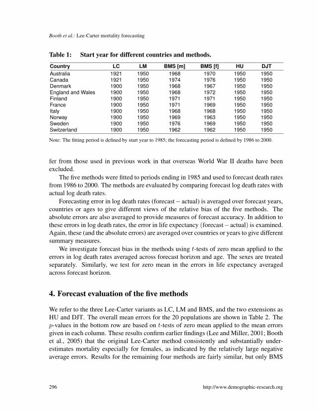
The data for this study are taken from the Human Mortality Database (2006). Ten coun-tries were selected giving 20 sex-specific populations for analysis. The ten countries se-lected are those with reliable data series commencing in 1921 or earlier. It was desirable touse only countries for which the available time series of data commenced somewhat ear-lier than 1950 in order to maintain the full and consistent comparison of the three variants.Lee and Carter (1992) used US data for the full period available, 1900–1989. Thereforethis multi-country analysis uses data for the period commencing in 1900 where possible.Though for some countries the data extend back to the nineteenth century, these weretruncated at 1900: the use of pre-1900 data would both reduce comparability of meth-ods across countries and necessitate a time series model with a non-linear trend whichfalls outside the scope of both applications to date and the current analysis. The selectedcountries are shown in Table 1 along with the dates used to define the fitting periods.

The data consist of central death rates and mid-year populations by sex and singleyears of age to 110 years. In the evaluation, data at older ages (age 95 and above) weregrouped in order to avoid problems associated with erratic rates at these ages. The eval-uation seeks to focus on the performance of methods in the context of reasonably regulardata rather than on their ability to cope with irregularities. The data for Australia dif-



Table 1: Start year for different countries and methods.

Country LC LM BMS [m] BMS [f] HU DJTAustralia 1921 1950 1968 1970 1950 1950Canada 1921 1950 1974 1976 1950 1950Denmark 1900 1950 1968 1967 1950 1950England and Wales 1900 1950 1968 1972 1950 1950Finland 1900 1950 1971 1971 1950 1950France 1900 1950 1971 1969 1950 1950Italy 1900 1950 1968 1968 1950 1950Norway 1900 1950 1969 1963 1950 1950Sweden 1900 1950 1976 1969 1950 1950Switzerland 1900 1950 1962 1962 1950 1950

Note: The fitting period is defined by start year to 1985; the forecasting period is defined by 1986 to 2000.

fer from those used in previous work in that overseas World War II deaths have beenexcluded.

The five methods were fitted to periods ending in 1985 and used to forecast death ratesfrom 1986 to 2000. The methods are evaluated by comparing forecast log death rates withactual log death rates.

Forecasting error in log death rates (forecast− actual) is averaged over forecast years,countries or ages to give different views of the relative bias of the five methods. Theabsolute errors are also averaged to provide measures of forecast accuracy. In addition tothese errors in log death rates, the error in life expectancy (forecast−actual) is examined.Again, these (and the absolute errors) are averaged over countries or years to give differentsummary measures.

We investigate forecast bias in the methods using t-tests of zero mean applied to theerrors in log death rates averaged across forecast horizon and age. The sexes are treatedseparately. Similarly, we test for zero mean in the errors in life expectancy averagedacross forecast horizon.

4. Forecast evaluation of the five methods

We refer to the three Lee-Carter variants as LC, LM and BMS, and the two extensions asHU and DJT. The overall mean errors for the 20 populations are shown in Table 2. Thep-values in the bottom row are based on t-tests of zero mean applied to the mean errorsgiven in each column. These results confirm earlier findings (Lee and Miller, 2001; Boothet al., 2005) that the original Lee-Carter method consistently and substantially under-estimates mortality especially for females, as indicated by the relatively large negativeaverage errors. Results for the remaining four methods are fairly similar, but only BMS



and HU show no evidence of bias in either female or male mortality. Sex differencesin this measure are related to the cancellation of positive and negative errors (compareTable 3).

Table 2: Overall mean error by sex, method and country. Mean taken over ageand year of the error in log death rates. The p-value is a test of bias (at-test for the average mean error to be zero).

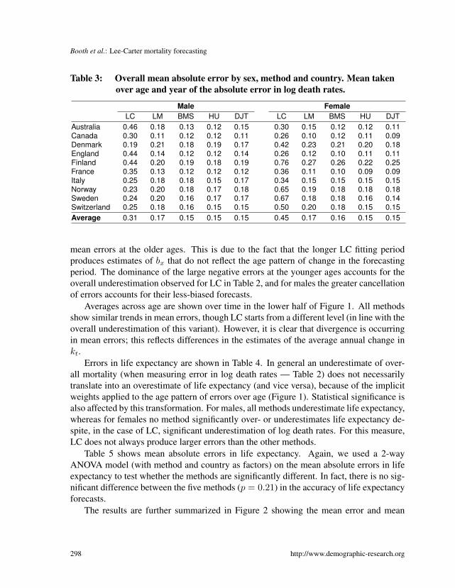
Male FemaleLC LM BMS HU DJT LC LM BMS HU DJT

Australia -0.23 0.10 0.04 0.00 0.08 -0.16 0.05 0.01 0.06 0.02Canada -0.13 0.04 -0.06 -0.07 0.04 -0.24 -0.03 -0.07 -0.08 -0.05Denmark 0.04 0.12 0.11 0.13 0.10 -0.36 0.04 0.03 0.03 0.02England -0.28 0.03 0.03 0.02 0.03 -0.20 0.00 0.02 0.00 -0.02Finland -0.24 0.01 -0.05 -0.02 -0.02 -0.68 -0.16 -0.17 -0.13 -0.17France -0.19 0.08 0.07 0.06 0.08 -0.27 0.02 0.03 0.02 0.02Italy -0.06 0.00 -0.03 0.02 0.01 -0.24 -0.06 -0.08 -0.05 -0.06Norway 0.17 0.10 0.11 0.07 0.09 -0.57 0.00 -0.04 -0.01 -0.05Sweden -0.09 0.06 -0.01 0.04 0.07 -0.61 -0.01 -0.04 -0.05 -0.03Switzerland -0.12 0.02 0.02 0.06 0.02 -0.44 -0.02 -0.03 0.02 -0.03Average -0.11 0.06 0.02 0.03 0.05 -0.38 -0.02 -0.03 -0.02 -0.03p-value 0.03 0.00 0.27 0.09 0.00 0.00 0.43 0.12 0.34 0.08

Table 3 provides a summary of forecast accuracy based on mean absolute error. Again,LC performs least well and there are only minor differences among the other four meth-ods. It is notable that the simple variations on the LC method used in LM and BMS pro-vide substantial improvements in forecast accuracy which are only marginally improvedby the more sophisticated HU and DJT methods. It is also notable that for this abso-lute measure, female and male mortality are equally difficult to forecast. Some countries(notably the Nordic countries) proved more difficult to forecast than others.

We used a 2-way ANOVA model (with method and country as factors) on the meanabsolute errors to test whether the methods are significantly different. A test for differ-ences between methods was highly significant (p < 0.001). However, using Tukey’sHonest Significant Differences to see which pairs of methods were different showed thatthe original LC method was significantly different from all other methods (p < 0.001),but the other four methods were not significantly different from each other (all p-valuesgreater than 0.86).

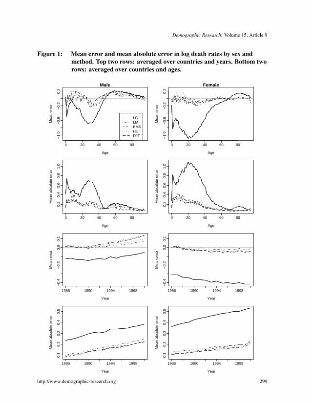
Age patterns of error in the log death rates are similar across countries; the average ofall countries is shown in Figure 1. There is a tendency for all methods to underestimatemortality for males aged 30–40 and overestimate mortality for males aged 45+. Similarly,all methods underestimate female mortality at ages 20–45. The LC method produces largenegative mean errors at the younger ages, particularly for females, and small positive



Table 3: Overall mean absolute error by sex, method and country. Mean takenover age and year of the absolute error in log death rates.


Australia 0.46 0.18 0.13 0.12 0.15 0.30 0.15 0.12 0.12 0.11Canada 0.30 0.11 0.12 0.12 0.11 0.26 0.10 0.12 0.11 0.09Denmark 0.19 0.21 0.18 0.19 0.17 0.42 0.23 0.21 0.20 0.18England 0.44 0.14 0.12 0.12 0.14 0.26 0.12 0.10 0.11 0.11Finland 0.44 0.20 0.19 0.18 0.19 0.76 0.27 0.26 0.22 0.25France 0.35 0.13 0.12 0.12 0.12 0.36 0.11 0.10 0.09 0.09Italy 0.25 0.18 0.18 0.15 0.17 0.34 0.15 0.15 0.15 0.15Norway 0.23 0.20 0.18 0.17 0.18 0.65 0.19 0.18 0.18 0.18Sweden 0.24 0.20 0.16 0.17 0.17 0.67 0.18 0.18 0.16 0.14Switzerland 0.25 0.18 0.16 0.15 0.15 0.50 0.20 0.18 0.15 0.15Average 0.31 0.17 0.15 0.15 0.15 0.45 0.17 0.16 0.15 0.15

mean errors at the older ages. This is due to the fact that the longer LC fitting periodproduces estimates of bx that do not reflect the age pattern of change in the forecastingperiod. The dominance of the large negative errors at the younger ages accounts for theoverall underestimation observed for LC in Table 2, and for males the greater cancellationof errors accounts for their less-biased forecasts.

Averages across age are shown over time in the lower half of Figure 1. All methodsshow similar trends in mean errors, though LC starts from a different level (in line with theoverall underestimation of this variant). However, it is clear that divergence is occurringin mean errors; this reflects differences in the estimates of the average annual change inkt.

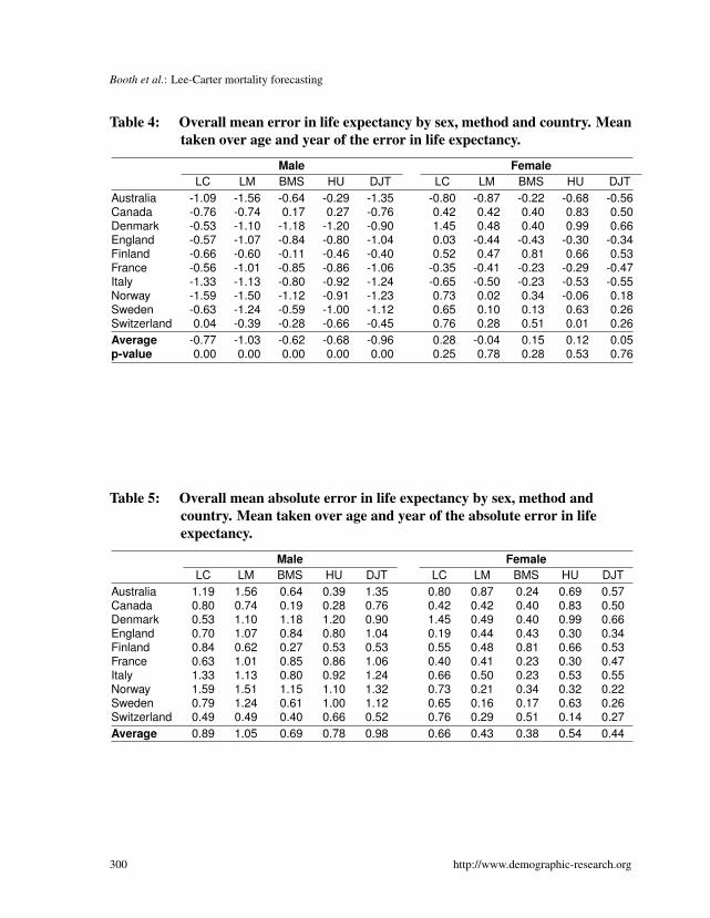
Errors in life expectancy are shown in Table 4. In general an underestimate of over-all mortality (when measuring error in log death rates — Table 2) does not necessarilytranslate into an overestimate of life expectancy (and vice versa), because of the implicitweights applied to the age pattern of errors over age (Figure 1). Statistical significance isalso affected by this transformation. For males, all methods underestimate life expectancy,whereas for females no method significantly over- or underestimates life expectancy de-spite, in the case of LC, significant underestimation of log death rates. For this measure,LC does not always produce larger errors than the other methods.

Table 5 shows mean absolute errors in life expectancy. Again, we used a 2-wayANOVA model (with method and country as factors) on the mean absolute errors in lifeexpectancy to test whether the methods are significantly different. In fact, there is no sig-nificant difference between the five methods (p = 0.21) in the accuracy of life expectancyforecasts.

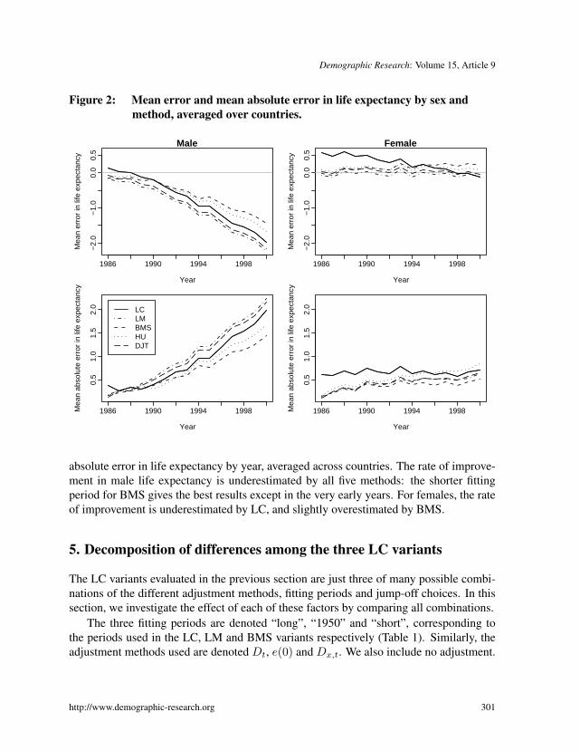
The results are further summarized in Figure 2 showing the mean error and mean



Figure 1: Mean error and mean absolute error in log death rates by sex andmethod. Top two rows: averaged over countries and years. Bottom tworows: averaged over countries and ages.

0 20 40 60 80

−1.

0−

0.6

−0.

20.

2

Male

Age

Mea

n er

ror

LCLMBMSHUDJT

0 20 40 60 80

−1.

0−

0.6

−0.

20.

2

Female

AgeM

ean

erro

r

0 20 40 60 80

0.2

0.4

0.6

0.8

1.0

Age

Mea

n ab

solu

te e

rror

0 20 40 60 80

0.2

0.4

0.6

0.8

1.0

Age

Mea

n ab

solu

te e

rror

1986 1990 1994 1998

−0.

4−

0.2

0.0

0.1

Year

Mea

n er

ror

1986 1990 1994 1998

−0.

4−

0.2

0.0

0.1

Year

Mea

n er

ror

1986 1990 1994 1998

0.1

0.2

0.3

0.4

0.5

Year

Mea

n ab

solu

te e

rror

1986 1990 1994 1998

0.1

0.2

0.3

0.4

0.5

Year

Mea

n ab

solu

te e

rror



Table 4: Overall mean error in life expectancy by sex, method and country. Meantaken over age and year of the error in life expectancy.


Australia -1.09 -1.56 -0.64 -0.29 -1.35 -0.80 -0.87 -0.22 -0.68 -0.56Canada -0.76 -0.74 0.17 0.27 -0.76 0.42 0.42 0.40 0.83 0.50Denmark -0.53 -1.10 -1.18 -1.20 -0.90 1.45 0.48 0.40 0.99 0.66England -0.57 -1.07 -0.84 -0.80 -1.04 0.03 -0.44 -0.43 -0.30 -0.34Finland -0.66 -0.60 -0.11 -0.46 -0.40 0.52 0.47 0.81 0.66 0.53France -0.56 -1.01 -0.85 -0.86 -1.06 -0.35 -0.41 -0.23 -0.29 -0.47Italy -1.33 -1.13 -0.80 -0.92 -1.24 -0.65 -0.50 -0.23 -0.53 -0.55Norway -1.59 -1.50 -1.12 -0.91 -1.23 0.73 0.02 0.34 -0.06 0.18Sweden -0.63 -1.24 -0.59 -1.00 -1.12 0.65 0.10 0.13 0.63 0.26Switzerland 0.04 -0.39 -0.28 -0.66 -0.45 0.76 0.28 0.51 0.01 0.26Average -0.77 -1.03 -0.62 -0.68 -0.96 0.28 -0.04 0.15 0.12 0.05p-value 0.00 0.00 0.00 0.00 0.00 0.25 0.78 0.28 0.53 0.76

Table 5: Overall mean absolute error in life expectancy by sex, method andcountry. Mean taken over age and year of the absolute error in lifeexpectancy.


Australia 1.19 1.56 0.64 0.39 1.35 0.80 0.87 0.24 0.69 0.57Canada 0.80 0.74 0.19 0.28 0.76 0.42 0.42 0.40 0.83 0.50Denmark 0.53 1.10 1.18 1.20 0.90 1.45 0.49 0.40 0.99 0.66England 0.70 1.07 0.84 0.80 1.04 0.19 0.44 0.43 0.30 0.34Finland 0.84 0.62 0.27 0.53 0.53 0.55 0.48 0.81 0.66 0.53France 0.63 1.01 0.85 0.86 1.06 0.40 0.41 0.23 0.30 0.47Italy 1.33 1.13 0.80 0.92 1.24 0.66 0.50 0.23 0.53 0.55Norway 1.59 1.51 1.15 1.10 1.32 0.73 0.21 0.34 0.32 0.22Sweden 0.79 1.24 0.61 1.00 1.12 0.65 0.16 0.17 0.63 0.26Switzerland 0.49 0.49 0.40 0.66 0.52 0.76 0.29 0.51 0.14 0.27Average 0.89 1.05 0.69 0.78 0.98 0.66 0.43 0.38 0.54 0.44



Figure 2: Mean error and mean absolute error in life expectancy by sex andmethod, averaged over countries.

1986 1990 1994 1998

−2.

0−

1.0

0.0

0.5

Male

Year

Mea

n er

ror

in li

fe e

xpec

tanc

y

1986 1990 1994 1998

−2.

0−

1.0

0.0

0.5

Female

YearM

ean

erro

r in

life

exp

ecta

ncy

1986 1990 1994 1998

0.5

1.0

1.5

2.0

Year

Mea

n ab

solu

te e

rror

in li

fe e

xpec

tanc

y

LCLMBMSHUDJT

1986 1990 1994 1998

0.5

1.0

1.5

2.0

Year

Mea

n ab

solu

te e

rror

in li

fe e

xpec

tanc

y

absolute error in life expectancy by year, averaged across countries. The rate of improve-ment in male life expectancy is underestimated by all five methods: the shorter fittingperiod for BMS gives the best results except in the very early years. For females, the rateof improvement is underestimated by LC, and slightly overestimated by BMS.

5. Decomposition of differences among the three LC variants

The LC variants evaluated in the previous section are just three of many possible combi-nations of the different adjustment methods, fitting periods and jump-off choices. In thissection, we investigate the effect of each of these factors by comparing all combinations.

The three fitting periods are denoted “long”, “1950” and “short”, corresponding tothe periods used in the LC, LM and BMS variants respectively (Table 1). Similarly, theadjustment methods used are denoted Dt, e(0) and Dx,t. We also include no adjustment.



The two jump-off choices are fitted rates (as in LC and BMS) or actual rates (as in LM)for jump-off. Thus we have 3× 4× 2 = 24 Lee-Carter variations.

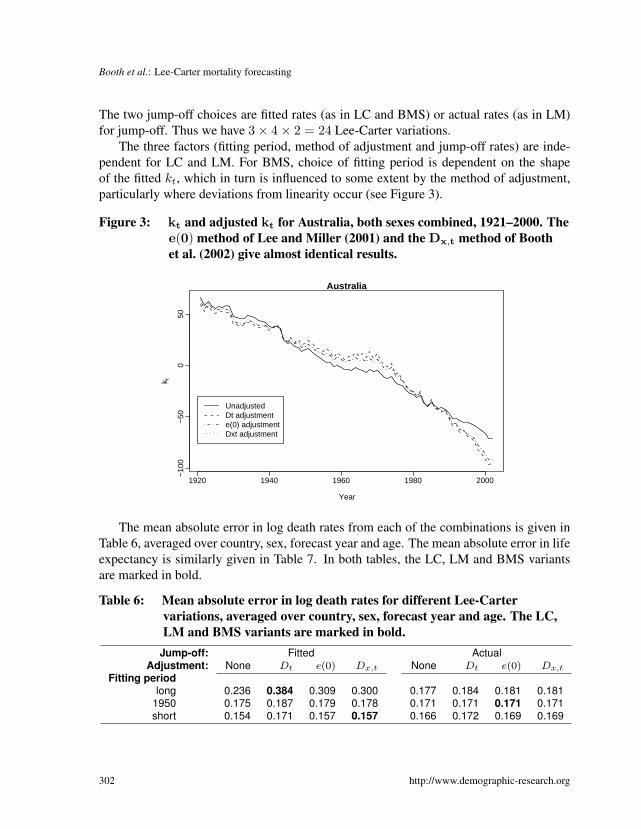
The three factors (fitting period, method of adjustment and jump-off rates) are inde-pendent for LC and LM. For BMS, choice of fitting period is dependent on the shapeof the fitted kt, which in turn is influenced to some extent by the method of adjustment,particularly where deviations from linearity occur (see Figure 3).

Figure 3: kt and adjusted kt for Australia, both sexes combined, 1921–2000. Thee(0) method of Lee and Miller (2001) and the Dx,t method of Boothet al. (2002) give almost identical results.

Australia

Year

k t

1920 1940 1960 1980 2000

−10

0−

500

50

UnadjustedDt adjustmente(0) adjustmentDxt adjustment

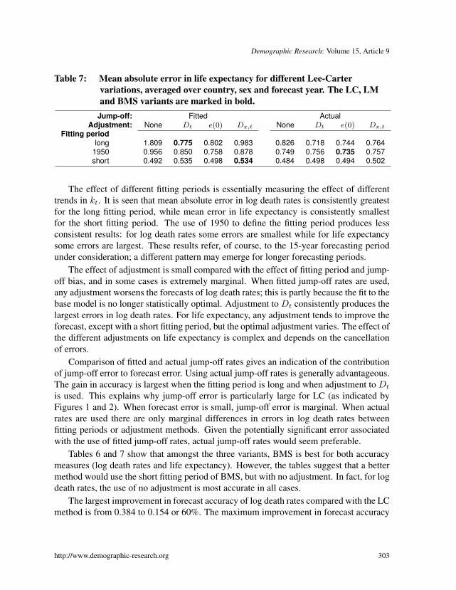
The mean absolute error in log death rates from each of the combinations is given inTable 6, averaged over country, sex, forecast year and age. The mean absolute error in lifeexpectancy is similarly given in Table 7. In both tables, the LC, LM and BMS variantsare marked in bold.

Table 6: Mean absolute error in log death rates for different Lee-Cartervariations, averaged over country, sex, forecast year and age. The LC,LM and BMS variants are marked in bold.

Jump-off: Fitted ActualAdjustment: None Dt e(0) Dx,t None Dt e(0) Dx,t

Fitting periodlong 0.236 0.384 0.309 0.300 0.177 0.184 0.181 0.181

1950 0.175 0.187 0.179 0.178 0.171 0.171 0.171 0.171short 0.154 0.171 0.157 0.157 0.166 0.172 0.169 0.169



Table 7: Mean absolute error in life expectancy for different Lee-Cartervariations, averaged over country, sex and forecast year. The LC, LMand BMS variants are marked in bold.

Jump-off: Fitted ActualAdjustment: None Dt e(0) Dx,t None Dt e(0) Dx,t

Fitting periodlong 1.809 0.775 0.802 0.983 0.826 0.718 0.744 0.764

1950 0.956 0.850 0.758 0.878 0.749 0.756 0.735 0.757short 0.492 0.535 0.498 0.534 0.484 0.498 0.494 0.502

The effect of different fitting periods is essentially measuring the effect of differenttrends in kt. It is seen that mean absolute error in log death rates is consistently greatestfor the long fitting period, while mean error in life expectancy is consistently smallestfor the short fitting period. The use of 1950 to define the fitting period produces lessconsistent results: for log death rates some errors are smallest while for life expectancysome errors are largest. These results refer, of course, to the 15-year forecasting periodunder consideration; a different pattern may emerge for longer forecasting periods.

The effect of adjustment is small compared with the effect of fitting period and jump-off bias, and in some cases is extremely marginal. When fitted jump-off rates are used,any adjustment worsens the forecasts of log death rates; this is partly because the fit to thebase model is no longer statistically optimal. Adjustment to Dt consistently produces thelargest errors in log death rates. For life expectancy, any adjustment tends to improve theforecast, except with a short fitting period, but the optimal adjustment varies. The effect ofthe different adjustments on life expectancy is complex and depends on the cancellationof errors.

Comparison of fitted and actual jump-off rates gives an indication of the contributionof jump-off error to forecast error. Using actual jump-off rates is generally advantageous.The gain in accuracy is largest when the fitting period is long and when adjustment to Dt

is used. This explains why jump-off error is particularly large for LC (as indicated byFigures 1 and 2). When forecast error is small, jump-off error is marginal. When actualrates are used there are only marginal differences in errors in log death rates betweenfitting periods or adjustment methods. Given the potentially significant error associatedwith the use of fitted jump-off rates, actual jump-off rates would seem preferable.

Tables 6 and 7 show that amongst the three variants, BMS is best for both accuracymeasures (log death rates and life expectancy). However, the tables suggest that a bettermethod would use the short fitting period of BMS, but with no adjustment. In fact, for logdeath rates, the use of no adjustment is most accurate in all cases.

The largest improvement in forecast accuracy of log death rates compared with the LCmethod is from 0.384 to 0.154 or 60%. The maximum improvement in forecast accuracy



of life expectancy rates is from 0.775 to 0.484 or 38%, but poorer accuracy also occurs(despite not occurring for log death rates).

By way of comparison, the mean absolute error in log death rates for HU is 0.149 andfor DJT is 0.150 (an improvement of 61% over LC in both cases). The mean absoluteerror in life expectancy for HU is 0.657 and for DJT it is 0.711. This is consistent withthe earlier findings, that HU and DJT are more accurate than the other methods in fore-casting log death rates, but this doesn’t translate into greater accuracy for life expectancyforecasts. An indication of the gain in accuracy attributable to the greater statistical so-phistication of HU and DJT can be obtained by comparing them with the four results for1950/fitted rates. The maximum gain in accuracy for HU is 20% for log death rates and31% for life expectancy. DJT achieves gains of up to 20% and 26% respectively.

6. Discussion and conclusions

The results of this comparative evaluation of forecasts for the period 1986–2000 showthat while each of the four variants and extensions is more accurate in forecasting logdeath rates than the original Lee-Carter method, none is consistently more accurate thanthe others. It was found that on average HU and DJT provided the most accurate forecastsof log death rates; however, the differences among the four methods are small and arenot significant. BMS provided marginally more accurate forecasts of life expectancy butthere were no significant differences between the five methods for this measure.

The changed ranking of methods depending on the measure of interest highlights theconceptual problem in defining forecast accuracy. Demographers have traditionally fo-cussed on life expectancy but, as has been seen, there is little relation between the relativeaccuracy of this measure and that of the underlying log death rates which are actuallymodelled. The two transformations, namely exponentiation and the life table (involvingthe cancellation of errors and implicit weights), are highly complex in combination suchthat the finer degree of accuracy in forecasting life expectancy is largely a matter of luck.Even if forecast life expectancy is accurate, compensating age-specific errors can be rel-atively substantial (see Figure 1) and in the long-term lead to unrealistic forecasts of theage pattern of mortality, with flow-on effects on forecasts of population structure. Whileaccuracy in forecasting life expectancy may be important, it is not sufficient. To gain anunderstanding of forecast error, the evaluation of error in log death rates is essential.

Among the factors defining the three Lee-Carter variants, it has been possible to iden-tify those that are generally advantageous. The shorter fitting periods of LM and BMSresult in greater accuracy on average than the longer fitting period, though earlier resultsshow that the ranking of LM and BMS in this respect differs by sex (Booth et al., 2005,Table 7). Actual jump-off rates generally do better than fitted jump-off rates, particularly



when the model is not a good fit to the data. However, there is no compelling evidencein favour of any of the adjustment methods. Further, among the possible combinations offactors, the combination of short fitting period, no adjustment of kt and fitted jump-offrates produced the smallest errors in log death rates (0.154) while actual jump-off rateswere more advantageous for life expectancy. Either of these combinations might thus beadopted at least for the short forecast horizons considered here.

There is some evidence that the absolute error in the log death rates increases asthe fitting period increases in length. This suggests that model misspecification may bepresent, probably due to the assumed linearity in modelling kt and the assumed fixed agepattern of change, bx. Given a changing pattern of mortality decline, such as occurredover the twentieth century, a shorter fitting period often results in more appropriate kt andbx for the forecasting period. This highlights the limitations of the model for longer fittingperiods. The random walk with drift model is in general a poor model for kt because itdoes not allow for dynamic changes in slope. Shorter fitting periods tend to work betterwith this model (at least for shorter forecast horizons) because they capture the mostrecent trend. Adaptive time series models such as those inherent in HU and DJT, whichplace more weight on recent than distant experience, tend to perform better for the samereason; our empirical results support this for the fifteen-year period in question. Similarly,the assumption of fixed bx is less of a limitation for shorter fitting periods because therecent pattern of change is most relevant. HU overcomes this assumption to some extentby the use of multiple functions, thus allowing for more flexible mortality changes.

It is noted that Tuljapurkar et al. (2000) did not adjust kt; they combined this withthe 1950 fitting period and fitted jump-off rates. The results of this evaluation show that,for 1950/fitted rates, the choice of no adjustment is advantageous for the accuracy offorecast log death rates but disadvantageous for the accuracy of life expectancy. Whilethese effects are moderate for the 1950 fitting period, they are substantial when the longfitting period is used. It is seen in Figure 3 that adjustment makes a noticeable differenceto the trend in kt: specifically, when no adjustment is used the decline is less rapid leadingto a lower fitted life expectancy in the jump-off year. This general pattern is observed forall ten populations included in this evaluation. (When the fitting period begins in 1950,adjustment makes little difference to the trend.) For life expectancy, the slower rate ofincrease from a lower jump-off point produces significant underestimation especially inthe longer term. Thus caution should be exercised in using no adjustment with longerfitting periods, especially when combined with fitted jump-off rates.

The results confirm the findings of Lee and Miller (2001) for a smaller group of pop-ulations. The LM use of actual jump-off rates in order to avoid jump-off bias is generallyendorsed. This is particularly important for very short horizons. In the longer term, jump-off bias becomes less important because it diminishes in size over time due to entropy ofthe life table. In contrast, error in the trend accumulates over time and quickly comes to



dominate total error (Figure 2). The indication that actual jump-off rates give greater fore-cast accuracy than fitted rates might be regarded as undermining the model. However, inall three Lee-Carter variants the model is already less than statistically optimal by virtueof the adjustment of kt. BMS and HU aim to reduce jump-off bias by achieving a betterfit to the underlying model; for HU this also involves the use of several basis functions.It is noted that the drift term of a random walk with drift is defined by the first and lastpoints of the fitting period. Thus the better the fit of the underlying model (or its firstbasis function) to the last point in particular, the smaller the jump-off bias and the moreaccurate the drift.

The LM variant is, in fact, widely referred to by Lee and others as the Lee-Cartermethod and it is this variant that is now widely applied. However, the original Lee-Carter method (specifically adjustment of kt to match total deaths) is still used as a pointof reference (e.g. Renshaw and Haberman, 2003c; Brouhns et al., 2002). This analysissuggests that not only is the original LC method a rather poor point of reference when theevaluation is focused on log death rates, but also that the LM variant is not the optimalpoint of reference (at least on the basis of these averaged results). Actual jump-off ratesand no adjustment of kt appears to be a better point of reference for all but the short fittingperiod where fitted rates are advantageous. Bongaarts (2005) uses as a reference the Lee-Carter method without adjustment. Actual rates may be replaced by the average observedrates over the last two or three years of the fitting period (Renshaw and Haberman, 2003a).

There has been no attempt in this paper to compare the five forecasting methods onany basis other than forecast accuracy. Further research is needed to compare forecastuncertainty among the five methods; a comparison of LC and BMS standard errors andprediction intervals appears in Booth et al. (2002). HU and DJT provide a general frame-work that is readily adapted to deal with more complex forecasting problems includingforecasting several populations with related dynamics such as a common trend. They alsoproduce forecast rates that are smooth across age, which may be an advantage in someapplications.

While the results are limited to the forecasting period and countries adopted, it islikely that they may be more widely generalised to other developed countries. The extentto which they may be generalised to other forecasting periods, including longer periods, isless clear. Other research comparing different forecasting methods has shown that forecastaccuracy is highly dependent on the particular period or population (e.g. Keyfitz, 1991;Murphy, 1995). In this comparison, however, the methods do not differ substantially,and it remains to be examined whether the details of the basic Lee-Carter method havea different effect in different forecasting periods. It is expected that the more flexiblemethods of HU and DJT will be better able to forecast less regular mortality patterns (e.g.where the time index does not show a linear trend). For the forecasting period adopted



and the countries included, however, these methods do not deliver a marked increase inforecast accuracy.

A final consideration is the ease with which the methods can be implemented. Tothis end, Hyndman (2006) is an R package which implements the HU, LC, LM and BMSmethods, as well as other variants of the Lee-Carter method.

7. Acknowledgments

We thank Len Smith for his assistance in handling various issues concerning the Aus-tralian data. We also thank Len and three reviewers for providing useful feedback andcomments on earlier versions of these results.



References

Bell W R. (1997). “Comparing and assessing time series methods for forecasting age-specific fertility and mortality rates.” Journal of Official Statistics, 13 (3): 279–303.

Bell W R, Monsell B. (1991), “Using principal components in time series modellingand forecasting of age-specific mortality rates.” In: Proceedings of the AmericanStatistical Association, Social Statistics Section, 154–159.

Bongaarts J. (2005). “Long-range trends in adult mortality: Models and projection meth-ods.” Demography, 42 (1): 23–49.

Booth H. (2006). “Demographic forecasting: 1980 to 2005 in review.” International Jour-nal of Forecasting, 22 (3), 547–581.

Booth H, Maindonald J, Smith L. (2002). “Applying Lee-Carter under conditions of vari-able mortality decline.” Population Studies, 56 (3): 325–336.

Booth H, Tickle L, Smith L. (2005). “Evaluation of the variants of the Lee-Carter methodof forecasting mortality: a multi-country comparison.” New Zealand Population Re-view, 31 (1): 13–34.

Brouhns N, Denuit M, Vermunt J K. (2002). “A Poisson log-bilinear regression approachto the construction of projected lifetables.” Insurance: Mathematics and Economics,31 (3): 373–393.

Buettner T, Zlotnik H. (2005). “Prospects for increasing longevity as assessed by theUnited Nations.” Genus, LXI (1): 213–233.

Currie I D, Durban M, Eilers P H C. (2004). “Smoothing and forecasting mortality rates.”Statistical Modelling, 4 (4): 279–298.

De Jong P, Tickle L. (2006). “Extending Lee-Carter mortality forecasting.” MathematicalPopulation Studies, 13 (1): 1–18.

Girosi F, King G. (2006), Demographic forecasting. Cambridge: Cambridge UniversityPress.

Harvey A C. (1989), Forecasting, structural time series models and the Kalman filter.Cambridge: Cambridge University Press.

Hastie T, Tibshirani R. (1990), Generalized additive models. London: Chapman &Hall/CRC.

Human Mortality Database. (2006). University of California, Berkeley (USA), and MaxPlanck Institute for Demographic Research (Germany), URL www.mortality.org, downloaded on 1 May 2006.



Hyndman R J, ed. (2006), demography: Forecasting mortality and fertility data. URLhttp://www.robhyndman.info/Rlibrary/demography, R package.

Hyndman R J, Koehler A B, Snyder R D, Grose S. (2002). “A state space framework forautomatic forecasting using exponential smoothing methods.” International Journalof Forecasting, 18 (3): 439–454.

Hyndman R J, Ullah M S. (2007). “Robust forecasting of mortality and fertility rates: afunctional data approach.” Computational Statistics and Data Analysis, to appear.

Keyfitz N. (1991). “Experiments in the projection of mortality.” Canadian Studies in Pop-ulation, 18 (2): 1–17.

Lee R D, Carter L R. (1992). “Modeling and forecasting U.S. mortality.” Journal of theAmerican Statistical Association, 87: 659–675.

Lee R D, Miller T. (2001). “Evaluating the performance of the Lee-Carter method forforecasting mortality.” Demography, 38 (4): 537–549.

Lee R D, Tuljapurkar S. (1994). “Stochastic population forecasts for the United States:beyond high, medium, and low.” Journal of the American Statistical Association,89: 1175–1189.

Li N, Lee R D, Tuljapurkar S. (2004). “Using the Lee-Carter method to forecast mortalityfor populations with limited data.” International Statistical Review, 72, 1: 19–36.

Lundström H, Qvist J. (2004). “Mortality forecasting and trend shifts: an application ofthe Lee–Carter model to Swedish mortality data.” International Statistical Review,72 (1): 37–50.

Lutz W, Goldstein J., ed. (2004), How to deal with uncertainty in population forecasting?IIASA Reprint Research Report RR-04-009. Reprinted from International Statisti-cal Review, 72 (1&2): 1–106, 157–208.

Makridakis S G, Wheelwright S C, Hyndman R J. (1998), “Forecasting: methods andapplications.” New York: John Wiley & Sons, 3rd edition.

Murphy M J. (1995). “The prospect of mortality: England and Wales and the UnitedStates of America, 1962–1989.” British Actuarial Journal, 1 (2): 331–350.

Ramsay J O, Silverman B W. (2005), “Functional data analysis.” New York: Springer-Verlag, 2nd edition.

Renshaw A E, Haberman S. (2003a). “Lee-Carter mortality forecasting: a parallel gen-eralized linear modelling approach for England and Wales mortality projections.”Applied Statistics, 52 (1): 119–137.



Renshaw A E, Haberman S. (2003b). “Lee-Carter mortality forecasting with age-specificenhancement.” Insurance: Mathematics and Economics, 33 (2): 255–272.

Renshaw A E, Haberman S. (2003c). “On the forecasting of mortality reduction factors.”Insurance: Mathematics and Economics, 32 (3): 379–401.

Trefethen L N, Bau D. (1997), “Numerical linear algebra.” Philadelphia: Society for In-dustrial and Applied Mathematics.

Tuljapurkar S, Li N, Boe C. (2000). “A universal pattern of mortality decline in the G7countries.” Nature, 405: 789–792.

Wilmoth J R. (1996), “Mortality projections for Japan: a comparison of four methods.”In: Caselli G, Lopez A, editors. Health and mortality among elderly populations.New York: Oxford University Press: 266–287.

Wood S.N. (2000), “Modelling and smoothing parameter estimation with multiplequadratic penalties.” Journal of the Royal Statistical Society, Series B, 62(2):413–428.


Date post:	15-May-2018
Category:	Documents
Upload:	trinhdat
View:	218 times
Download:	0 times

Lee-Carter mortality forecasting: a multi-country comparison … · Lee-Carter mortality...

Documents