Abstract. We present a new sublinear-size index structure for finding all occurrences of a givenq-gram ina text. Such aq-gram index is needed in many approximate pattern matching algorithms. All earlierq-gramindexes require at leastO(n) space, wheren is the length of the text. The new Lempel–Ziv index needs onlyO(n/logn) space while being as fast as previous methods. The new method takes advantage of repetitions inthe text found by Lempel–Ziv parsing.
Key Words. q-Gram index, Approximate pattern matching, Text indexing, Lempel–Ziv parsing, Stringalgorithms, Data compression.
1. Introduction. The approximate pattern matching problemis as follows. Given atext T = T [1, n] and apatternP = P[1,m] in an alphabet6 and an integerk,find all the text positionsi such that an approximate occurrence ofP with at mostkdifferences ends ati . The difference between two stringsα andβ is measured as theeditdistance d: d(α, β) is the minimum number ofedit operations(insertions, deletions,or changes) needed to convertα to β (or, equivalently,β to α). Approximate patternmatching has several applications, for example, in textual databases, biocomputing, datacommunications, and data mining.
Filtration with q-Grams. The basic solution for the approximate pattern matchingproblem is based on dynamic programming [10], [20]. It hasO(kn) time complexitywhich is often too slow for long texts. Therefore, severalfiltration schemes have beenintroduced in order to extract the text areas with potential matches, to be inspected bydynamic programming in the second phase of the algorithm. Each filtration scheme isbased on its specificfiltration condition, stating a necessary condition for an approximatematch.
There are several possible ways to express the filtration condition. Potential approxi-mate matches can be recognized by character distributions [6], locating matching blocksof the pattern in the text [23], retrieving maximal matching substrings of the pattern inthe text [4], [21], or even applying the Boyer–Moore idea of exact pattern matching [2]to the approximate pattern matching [19].
A very popular family of filtration schemes, called theq-family, states the filtrationcondition in terms ofq-grams. By a q-gram, we refer to any (sub)string ofq charac-ters. For example, patternMOROGOROhas 3-gramsMOR, ORO, ROG, OGO, andGOR. Anapproximate match resembles the original pattern and must, therefore, contain at least
1 This work was supported by the Academy of Finland.2 Department of Computer Science, P.O. Box 26 (Teollisuuskatu 23), FIN-00014 University of Helsinki,Finland.{Juha.Karkkainen,Erkki.Sutinen}@cs.Helsinki.FI.
Received November 1996; revised March 1997. Communicated by J. D´ıaz and M. J. Serna.
138 J. Karkkainen and E. Sutinen
some commonq-grams with the pattern. This similarity has been used in many differentways in theq-gram filtration schemes. However, common to all of them is that the textq-grams that match the patternq-grams must be found. This can be done in two differentways. Thedynamicapproach scans the text in linear time, while thestatic approachutilizes aq-gram index. The static approach is superior when the sameq-gram indexcan be used several times.
The classical paper by Jokinen and Ukkonen [8], introducing the use ofq-grams inpattern matching, presented a static algorithm. Among the last members in theq-family,we name the dynamic approaches by Ukkonen [21], Chang and Marr [5], Takaoka [18],and Sutinen and Tarhio [16], [17]. Static algorithms have been introduced by Myers [14],Holsti and Sutinen [7], and Sutinen and Tarhio [17]. Furthermore, the FLASH system[3], designed for approximate pattern matching in biological data, appliesq-grams in aprobabilistic algorithm. In addition,q-grams have been applied in information retrievalschemes [1], [11].
Current Implementations of q-Gram Indexes. A q-gram index of a text needed in thestaticq-gram methods is a data structure that allows one to find all occurrences of agiven q-gram in the text quickly. The basic implementation is a pointer array of size|6|q. Each entry of the array holds a list of the occurrences of the correspondingq-gramin the text. The index can be built in timeO(n+ |6|q) [8].
The problem with this approach is the exponential dependence of the size of the arrayon q. This results in unnecessarily large indexes, especially when only a small fractionof potentialq-grams occurs in the text. This is true, e.g., for natural language texts andall cases wheren¿ |6|q.
A natural improvement of the indexing scheme stated above is to reduce the size ofthe pointer array by hashing. By a suitable selection of the hash function, the size andconstruction time are reduced toO(n) without significant slowdown in searching.
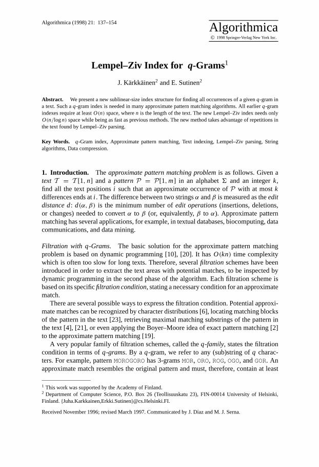
A different solution to the indexing problem uses a trie structure. The textq-gramsare stored into a trie, with each leaf storing a list of the occurrences of the correspondingq-gram in the text (Figure 1). The trie can be built inO(n) time, for example, by usingan algorithm similar to creating a suffix tree [22].
All the above implementations can find all occurrences of a givenq-gram in optimalO(q+l ) time, wherel is the number of occurrences found. However, the implementationssuffer from the same drawback: because of the at least linear space consumption, the
Fig. 1. Comparison of trie implementations of a traditional 3-gram index and the new Lempel–Ziv index for3-grams.
Lempel–Ziv Index forq-Grams 139
size of the index gets unpractically large with an increasing text lengthn. The hashingand trie structures can actually be implemented inO(M) space, whereM , the number ofdistinctq-grams of the text, can be much less thann. However, the lists of occurrencesalways requireO(n) space.
Sketch of the New q-Gram Index. In the new Lempel–Ziv (LZ) index forq-grams, thelists of occurrences are replaced with a data structure that provides the same informationin a more compact form (Figure 1). The (hashing or trie) structure for the distinctq-grams, called theprimary index, is still needed for providing a starting point for thesearch.
The compact representation of the occurrence lists takes advantage of repetitions inthe text. With arepetitionwe mean a string that occurs (at least) twice in the text. Thefirst occurrence is called thedefinition and the later occurrence is called thephrase.Every occurrence of aq-gram is either the first of its kind or a part of some phrase.The first occurrences can be stored in the primary index, e.g., in the leaves of a trie. Allother occurrences are found using information about repetitions. Space is saved becausea long repetition can represent severalq-grams.
As an example, consider Figure 2. The first occurrence of theq-gramQ is found usingthe primary index. This phase of the algorithm is called theprimary search. Next, we findthe two definitions that contain the first occurrence. Just by using the information aboutrepetitions, we can then deduce the locations of the second and fourth occurrence. Thisis called thesecondary search. In the tertiary searchwe find the definition containingthe second occurrence which then leads to finding the third occurrence.
The tertiary search is applied for every newq-gram occurrence found. The differencebetween the secondary search and the tertiary search is that we can have precomputedinformation associated with the first occurrence to provide a starting point for the sec-ondary search. The starting point for a tertiary search is the phrase that contains thecurrent occurrence. However, this starting point is common to all theq-grams withinthat phrase, which makes searching a little more difficult.
The repetitions in the text are found by a variation of Lempel–Ziv parsing. Lempel–Ziv parsing is also used in Ziv–Lempel text compression methods, where phrases arereplaced with pointers to their definitions [24]. Our use of Lempel–Ziv parsing couldbe described as compressing the lists of occurrences instead of the text. Similar ideas,leading to quite different data structures, were used in [9] for exact pattern matching.
The LZ index can find all occurrences of a givenq-gram inO(q+ l ) time, the sameas traditionalq-gram indexes. The size of the LZ index isO(M + N), whereM is thenumber of distinctq-grams in the text andN is the number of repetitions needed to
Fig. 2. The idea of the new method. The dark rectangles show the locations of aq-gramQ. A pair of lines,connected by an arrow, represents two occurrences of the same string (a repetition). The thick line is thedefinition and the thin line is the phrase.
140 J. Karkkainen and E. Sutinen
cover allq-grams except the first occurrence of each distinctq-gram. Obviously,M+Nis at mostn, but it can be significantly less. In Section 8 we give conditions for thesize to be sublinear. For example, ifq is constant or grows slow enough withn, thenM+N = O(n/logn). The size also decreases when the repetitiveness (compressibility)of the text increases.
In the next section we describe Lempel–Ziv parsing. Then, in Section 3, we give anoutline of the search algorithm. The new data structures are based on certain combinato-rial properties of intervals. These are studied in Section 4. The actual data structures arepresented in Section 5 for the secondary search and in Section 6 for the tertiary search.The construction of the data structures is described in Section 7. In Section 8 we givetheoretical and experimental results on the size of the new index, and then, in Section 9,compare the new scheme with traditional approaches. Finally, in Section 10, we pointout some aspects needing further research.
2. Lempel–Ziv Parsing. Let the stringT = t1t2 · · · tn be the text. We useT [i, j ] todenote the substringti ti+1 · · · tj of T . The notation [i, j ] denotes anintervaland can, inthis paper, be interpreted to refer to the substringti ti+1 · · · tj with its content unknownor irrelevant. That is, [i, j ] denotes thepositionrather than the content. An alternativenotation that is used frequently in this paper is [i → l ] = [i, i + l − 1].
The new index utilizes repetitions in the text to reduce the space requirement of theq-gram index. The information about the repetitions is represented by an LZ parse.
DEFINITION 1. Lempel–Ziv(LZ) parsefor a textT is a set of triplets(Ii , Ji , Li ), i =1, . . . , N, whereIi > Ji andT [ Ii → Li ] = T [ Ji → Li ].
The intervals [Ii → Li ] are calledphrasesand [Ji → Li ] are calleddefinitions. Thephrases and definitions are defined as intervals rather than substrings because the onlyessential information about their content is that, for alli , [ Ii → Li ] and [Ji → Li ] havethe same content.
LZ parsing was originally used for measuring the complexity of a text [12]. The bestknown application of LZ parsing is Ziv–Lempel compression, where the contents ofphrases are replaced with references to definitions [24]. Our use of the LZ parse utilizesthe identityT [ Ii → Li ] = T [ Ji → Li ] in a different way.
If there is an occurrence of aq-gramQ inside the phrase [Ii → Li ], there is anoccurrence ofQwithin the definition [Ji → Li ], too. The two occurrences are called thephrase occurrenceand itsdefinition, respectively. In the LZ index, phrase occurrencesare found through their definitions. A definition of a phrase occurrence may itself bea phrase occurrence and have its own definition. Circular definitions are not possible,however, due to the conditionIi > Ji .
Definition 1 does not specify how to choose the phrases and definitions. In the originalLZ parsing the phrases are formed starting from the beginning of the text so that eachphrase begins where the previous phrase ends3 and is as long as Definition 1 allows. Theidea is to cover as much of the text as possible with as few phrases as possible.
3 To be exact, there is one character between consecutive phrases.
Lempel–Ziv Index forq-Grams 141
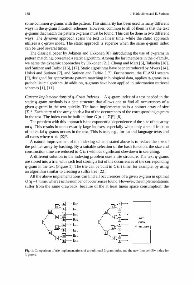
Fig. 3.An example of LZ parsing by Algorithm 1 withq = 3. The text is at the top. The rest of the lines showthe phrases (white background) and the noncovered 3-grams (gray background) in the order they are formedby Algorithm 1. The definitions are shown by boxes on the line of the corresponding phrases. The output ofAlgorithm 1 in this case is{(4, 1, 3), (6, 1, 11), (15, 2, 6), (21, 15, 11), (30, 2, 3)}, {1, 2, 3, 5, 19, 20}.
Our goal is to cover as manyq-grams as possible with as few phrases as possible.The phrases are computed in the same way as in the original LZ parsing except thatconsecutive phrases overlap byq − 1 characters. In detail, the method is described inAlgorithm 1. Forq = 0, Algorithm 1 computes exactly the original LZ parse. Thealgorithm also computes the starting positions of the noncoveredq-grams. An exampleof the operation of Algorithm 1 is shown in Figure 3.
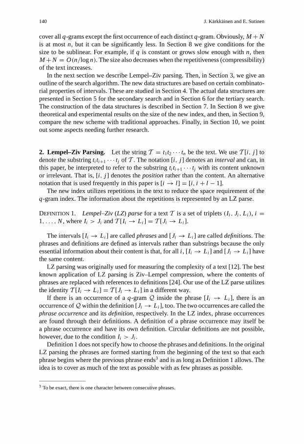
Algorithm 1: LZPARSE
Input: textT of lengthnOutput: LZ parse of textT , starting positions of all noncoveredq-grams
1 i ← j ← I1← 12 while Ii ≤ n− q + 1 do3 Li ← max{L | ∃J < Ii : T [ J → L] = T [ Ii → L]}4 if Li < q then % noncoveredq-gram5 Pj ← Ii
6 j ← j + 17 Ii ← Ii + 18 else % phrase9 Ji ← min{J | T [ J → Li ] = T [ Ii → Li ]}
10 Ii+1← Ii + Li − q + 111 i ← i + 112 N ← i − 113 M ← j − 114 return {(I1, J1, L1), . . . , (IN, JN, L N)}, {P1, . . . , PM}
142 J. Karkkainen and E. Sutinen
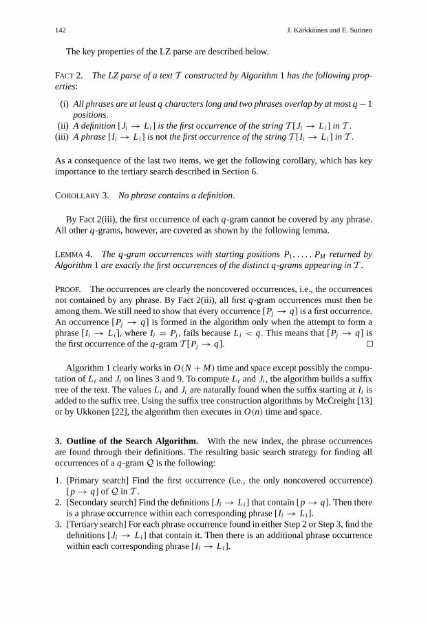
The key properties of the LZ parse are described below.
FACT 2. The LZ parse of a textT constructed by Algorithm1 has the following prop-erties:
(i) All phrases are at least q characters long and two phrases overlap by at most q−1positions.
(ii) A definition[ Ji → Li ] is the first occurrence of the stringT [ Ji → Li ] in T .(iii) A phrase[ Ii → Li ] is not the first occurrence of the stringT [ Ii → Li ] in T .
As a consequence of the last two items, we get the following corollary, which has keyimportance to the tertiary search described in Section 6.
COROLLARY 3. No phrase contains a definition.
By Fact 2(iii), the first occurrence of eachq-gram cannot be covered by any phrase.All other q-grams, however, are covered as shown by the following lemma.
LEMMA 4. The q-gram occurrences with starting positions P1, . . . , PM returned byAlgorithm1 are exactly the first occurrences of the distinct q-grams appearing inT .
PROOF. The occurrences are clearly the noncovered occurrences, i.e., the occurrencesnot contained by any phrase. By Fact 2(iii), all firstq-gram occurrences must then beamong them. We still need to show that every occurrence [Pj → q] is a first occurrence.An occurrence [Pj → q] is formed in the algorithm only when the attempt to form aphrase [Ii → Li ], where Ii = Pj , fails becauseLi < q. This means that [Pj → q] isthe first occurrence of theq-gramT [ Pj → q].
Algorithm 1 clearly works inO(N +M) time and space except possibly the compu-tation ofLi andJi on lines 3 and 9. To computeLi andJi , the algorithm builds a suffixtree of the text. The valuesLi andJi are naturally found when the suffix starting atIi isadded to the suffix tree. Using the suffix tree construction algorithms by McCreight [13]or by Ukkonen [22], the algorithm then executes inO(n) time and space.
3. Outline of the Search Algorithm. With the new index, the phrase occurrencesare found through their definitions. The resulting basic search strategy for finding alloccurrences of aq-gramQ is the following:
1. [Primary search] Find the first occurrence (i.e., the only noncovered occurrence)[ p→ q] of Q in T .
2. [Secondary search] Find the definitions [Ji → Li ] that contain [p→ q]. Then thereis a phrase occurrence within each corresponding phrase [Ii → Li ].
3. [Tertiary search] For each phrase occurrence found in either Step 2 or Step 3, find thedefinitions [Ji → Li ] that contain it. Then there is an additional phrase occurrencewithin each corresponding phrase [Ii → Li ].
Lempel–Ziv Index forq-Grams 143
Note that to determine containment in Steps 2 and 3, it is only necessary to comparethe endpoints; no character comparisons are needed. The difference between secondaryand tertiary searches will be explained shortly.
EXAMPLE 1. Applying the search to find the occurrences ofbba in the text of Figure 3works as follows. First, in the primary search, we find the only noncovered occurrenceat [3, 5]. Next, in the secondary search, we find that the definitions [1, 11] and [2, 7]contain the first occurrence. The corresponding phrases are [6, 16] and [15, 20], respec-tively, from which we see that there are occurrences at [8, 10] and [16, 18], respectively.Similarly, the tertiary search then proceeds as follows:
[8, 10] ⊆ [1, 11] ⇒ occurrence at [13, 15]⊆ [6, 16],[16, 18] ⊆ [15, 25] ⇒ occurrence at [22, 24]⊆ [21, 31],[13, 15] is contained by no definition.[22, 24] ⊆ [15, 25] ⇒ occurrence at [28, 30]⊆ [21, 31],[28, 30] is contained by no definition.
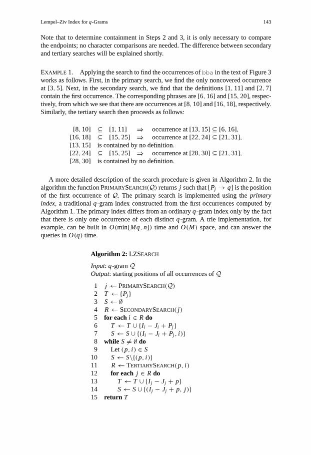
A more detailed description of the search procedure is given in Algorithm 2. In thealgorithm the function PRIMARYSEARCH(Q) returnsj such that [Pj → q] is the positionof the first occurrence ofQ. The primary search is implemented using theprimaryindex, a traditionalq-gram index constructed from the first occurrences computed byAlgorithm 1. The primary index differs from an ordinaryq-gram index only by the factthat there is only one occurrence of each distinctq-gram. A trie implementation, forexample, can be built inO(min{Mq, n}) time andO(M) space, and can answer thequeries inO(q) time.
Algorithm 2: LZSEARCH
Input: q-gramQOutput: starting positions of all occurrences ofQ
1 j ← PRIMARYSEARCH(Q)2 T ← {Pj }3 S← ∅4 R← SECONDARYSEARCH( j )5 for each i ∈ R do6 T ← T ∪ {Ii − Ji + Pj }7 S← S∪ {(Ii − Ji + Pj , i )}8 while S 6= ∅ do9 Let (p, i ) ∈ S
10 S← S\{(p, i )}11 R← TERTIARYSEARCH(p, i )12 for each j ∈ R do13 T ← T ∪ {I j − Jj + p}14 S← S∪ {(I j − Jj + p, j )}15 return T
144 J. Karkkainen and E. Sutinen
The function SECONDARYSEARCH( j ) in Algorithm 2 computes alli such that thedefinition [Ji → Li ] contains [Pj → q]. To make the secondary search fast, we associatesome extra information, a starting point to the secondary search, to each of theMnoncoveredq-gram occurrences. The implementation is described in Section 5.
The function TERTIARYSEARCH(p, i ) computes allj such that the definition [Jj →L j ] contains [p→ q], when [p→ q] is known to be contained by the phrase [Ii → Li ].The tertiary search differs from the secondary search in that the starting point to the searchis associated with the the phrase [Ii → Li ] instead of the occurrence [p → q]. Thismakes tertiary search somewhat more difficult since a starting point is not unique to[ p→ q]. The implementation is described in Section 6.
4. Intervals. The secondary and tertiary search problems above were stated in terms ofdefinitions, phrases, andq-grams occurrences, all of which are intervals. Our secondaryand tertiary search algorithms are based on some combinatorial properties of intervals.In this section we describe these key properties.
We start by defining two partial orders on intervals.
DEFINITION 5. An interval [I , J] is containedby an interval [I ′, J ′], denoted by [I , J] ⊆[ I ′, J ′], iff I ′ ≤ I andJ ≤ J ′. There are two degrees of inequality:
[ I , J] ⊂ [ I ′, J ′] iff [ I , J] ⊆ [ I ′, J ′] and [I , J] 6= [ I ′, J ′],
[ I , J] ≺ [ I ′, J ′] iff [ I , J] ⊆ [ I ′, J ′], I 6= I ′, and J 6= J ′.
In the last case, we say that [I , J] is nestedwithin [ I ′, J ′].
DEFINITION 6. An interval [I , J] precedesan interval [I ′, J ′], denoted by [I , J] ≤[ I ′, J ′], iff I ≤ I ′ andJ ≤ J ′. There are two degrees of inequality:
[ I , J] < [ I ′, J ′] iff [ I , J] ≤ [ I ′, J ′] and [I , J] 6= [ I ′, J ′],[ I , J] ¿ [ I ′, J ′] iff [ I , J] ≤ [ I ′, J ′], I 6= I ′, and J 6= J ′.
Two intervals [I , J] and [I ′, J ′] arecomparablein ⊆ (≤) iff [ I , J] ⊆ (≤)[ I ′, J ′] or[ I ′, J ′] ⊆ (≤) [ I , J]. Otherwise, [I , J] and [I ′, J ′] are incomparablein ⊆ (≤).
EXAMPLE 2. [3, 4] ≺ [2, 5] ⊂ [2, 7], but [1, 3] and [2, 5] are incomparable in⊆.[1, 3]¿ [2, 5] < [2, 7], but [2, 5] and [3, 4] are incomparable in≤.
The two partial orders are related by the following lemma.
LEMMA 7 (Orthogonality). Two intervals[ I , J] and[ I ′, J ′] are always comparable ineither⊆ or ≤. The intervals are comparable in both⊆ and≤ iff I = I ′ or J = J ′.
We say that⊆ and≤ areorthogonal.
COROLLARY 8. Two intervals[ I , J] and [ I ′, J ′] are incomparable in≤ iff [ I , J] ≺[ I ′, J ′] or [ I ′, J ′] ≺ [ I , J].
Lempel–Ziv Index forq-Grams 145
The basic idea of our algorithms for secondary and tertiary search is to sort thedefinitions by≤. The order≤ is a partial order, but Corollary 8 allows us to partition theset of definitions into sets for which≤ is a total order.
DEFINITION 9. LetS be a set of intervals. Thenesting levelof an interval [I , J] in S,denoted bynlS([ I , J]), is the largest integerk for which there exists a set{[ I1, J1], . . . ,[ Ik, Jk]} ⊂ S such that [I , J] ≺ [ I1, J1] ≺ · · · ≺ [ Ik, Jk].
Let NLk(S) denote the set of intervals ofS with nesting levelk in S, i.e.,NLk(S) ={[ I , J] ∈ S | nlS([ I , J]) = k}. Let H be the largest integer for whichNLH (S) isnonempty. ThenNL0(S),NL1(S), . . . ,NLH (S) is called thenesting level partitionof S.The key property of nesting levels is the following.
THEOREM10. LetS be a set of intervals and let k be a nonnegative integer. Then≤ isa total order for NLk(S).
PROOF. Let [I , J] and [I ′, J ′] be intervals inNLk(S). Assume, contradictory to thetheorem, that [I , J] and [I ′, J ′] are incomparable in≤. Then, by Corollary 8, [I , J] ≺[ I ′, J ′] or [ I ′, J ′] ≺ [ I , J]. Assume [I , J] ≺ [ I ′, J ′]. By Definition 9, [I ′, J ′] ≺[ I1, J1] ≺ · · · ≺ [ Ik, Jk] for some{[ I1, J1], . . . , [ Ik, Jk]} ⊂ S. Then [I , J] ≺ [ I ′, J ′] ≺[ I1, J1] ≺ · · · ≺ [ Ik, Jk] and thereforenlS([ I , J]) > k, i.e., [I , J] 6∈ N Lk(S).
5. Secondary Search. The secondary search problem can be stated as follows:
Given the first occurrence of theq-gramQ in the textT at position [p→ q], findall definitions [Ji → Li ], i = 1, . . . , N, that contain [p→ q].
As can be seen from this formulation, the problem is concerned with intervals ratherthan strings. In fact, neither the textT nor theq-gramQ are needed at all.
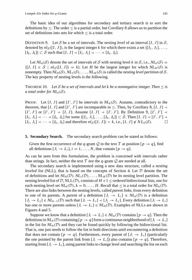
The secondary search is implemented using a new data structure, called anestingleveled list(NLL), that is based on the concepts of Section 4. LetD denote the setof definitions and letNL0(D),NL1(D), . . . ,NLH (D) be its nesting level partition. Thenesting leveled list ofD, NLL(D), consists ofH+1≤-ordered bidirectional lists, one foreach nesting level setNLk(D), k = 0, . . . , H . Recall that≤ is a total order forNLk(D).There are also links between the nesting levels, calledparent links, from every definitionto one of its parents. Aparent of a definition [Ji → Li ] ∈ NLk(D) is a definition[ Jj → L j ] ∈ NLk−1(D) such that [Ji → Li ] ≺ [ Jj → L j ]. Every definition [Ji → Li ]has one or more parents unless [Ji → Li ] ∈ NL0(D). Examples of NLLs are shown inFigures 4 and 5.
Suppose we know that a definition [Ji → Li ] ∈ NLk(D) contains [p→ q]. Then thedefinitions inNLk(D) containing [p→ q] form a continuous neighborhood of [Ji → Li ]in the list forNLk(D) and they can be found quickly by following the bidirectional list.That is, one just needs to follow the list in both directions until encountering a definitionthat does not contain [p → q]. Furthermore, every parent of [Ji → Li ] (particularlythe one pointed by the parent link from [Ji → Li ]) also contains [p→ q]. Therefore,starting from [Ji → Li ], using parent links to change level and searching the list on each
146 J. Karkkainen and E. Sutinen
Fig. 4.Two representations of the nesting leveled list for the LZ parse of Figure 3.
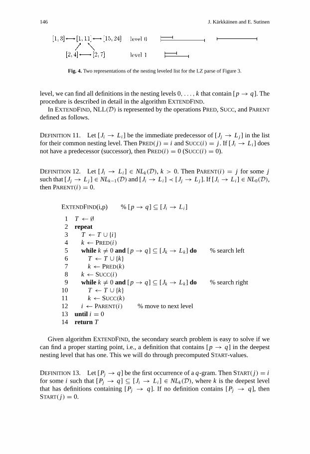
level, we can find all definitions in the nesting levels 0, . . . , k that contain [p→ q]. Theprocedure is described in detail in the algorithm EXTENDFIND.
In EXTENDFIND, NLL(D) is represented by the operations PRED, SUCC, and PARENT
defined as follows.
DEFINITION 11. Let [Ji → Li ] be the immediate predecessor of [Jj → L j ] in the listfor their common nesting level. Then PRED( j ) = i and SUCC(i ) = j . If [ Ji → Li ] doesnot have a predecessor (successor), then PRED(i ) = 0 (SUCC(i ) = 0).
DEFINITION 12. Let [Ji → Li ] ∈ NLk(D), k > 0. Then PARENT(i ) = j for some jsuch that [Jj → L j ] ∈ NLk−1(D) and [Ji → Li ] ≺ [ Jj → L j ]. If [ Ji → Li ] ∈ NL0(D),then PARENT(i ) = 0.
EXTENDFIND(i,p) % [p→ q] ⊆ [ Ji → Li ]
1 T ← ∅2 repeat3 T ← T ∪ {i }4 k← PRED(i )5 while k 6= 0 and [ p→ q] ⊆ [ Jk → Lk] do % search left6 T ← T ∪ {k}7 k← PRED(k)8 k← SUCC(i )9 while k 6= 0 and [ p→ q] ⊆ [ Jk → Lk] do % search right
10 T ← T ∪ {k}11 k← SUCC(k)12 i ← PARENT(i ) % move to next level13 until i = 014 return T
Given algorithm EXTENDFIND, the secondary search problem is easy to solve if wecan find a proper starting point, i.e., a definition that contains [p → q] in the deepestnesting level that has one. This we will do through precomputed START-values.
DEFINITION 13. Let [Pj → q] be the first occurrence of aq-gram. Then START( j ) = ifor somei such that [Pj → q] ⊆ [ Ji → Li ] ∈ NLk(D), wherek is the deepest levelthat has definitions containing [Pj → q]. If no definition contains [Pj → q], thenSTART( j ) = 0.
Lempel–Ziv Index forq-Grams 147
The algorithm SECONDARYSEARCH now solves the secondary search problem.
SECONDARYSEARCH(j) % [ Pj → q] is an occurrence
1 i ← START( j )2 if i = 0 then return ∅3 else returnEXTENDFIND(i, Pj )
Each execution of a loop body in EXTENDFIND adds a new definition containing[ p → q] into T and each of the definitions inT will lead to a discovery of a newoccurrence. Therefore, the whole secondary search runs in linear time in the number ofoccurrences found. The size of the nesting leveled list isO(N), and the START pointersrequireO(M) space. The construction of the data structures is described in Section 7.
6. Tertiary Search. The tertiary search problem is very similar to the secondary searchproblem:
Given an occurrence of theq-gramQ in the textT at a position [p→ q] containedby a phrase [Ii → Li ], find all definitions [Jj → L j ], j = 1, . . . , N, that contain[ p→ q].
There are two differences when compared with the secondary search. First, the occurrenceat [p→ q] is not a first occurrence, and, second, we know the phrase that contains theoccurrence. The procedure EXTENDFIND can be used for tertiary search, too, but theproblem is to find a proper starting point. Associating a precomputed starting point withevery possible phrase occurrence would defeat the purpose of saving space. Instead, wewill find the starting point through the phrase [Ii → Li ] that is known to contain theoccurrence [p→ q].
Recall that a proper starting point is a definition that contains [p→ q] at the deepestnesting level that has one. Here, the potential starting points are the definitions thatoverlap the phrase [Ii → Li ] by at leastq positions. Any such definition [Jj → L j ] canbe classified into one of the following categories with respect to the phrase [Ii → Li ]:
1. Contained definition: [Jj → L j ] ⊆ [ Ii → Li ]
2. Containing definition: [Ii → Li ] ⊂ [ Jj → L j ]
3. Preceding definition: [Jj → L j ] ¿ [ Ii → Li ]
4. Succeeding definition: [Ii → Li ] ¿ [ Jj → L j ]
The first category must be empty, due to Corollary 3. The second category definitionsare guaranteed to contain the occurrence [p → q]. The preceding and succeedingdefinitions may or may not contain [p→ q].
Let Ki be the deepest nesting level that has a definition containing [Ii → Li ] andlet Hi be the deepest nesting level that has a preceding or succeeding definition with anoverlap of at leastq. Then all nesting levels 0, . . . , Ki have a definition that contains
148 J. Karkkainen and E. Sutinen
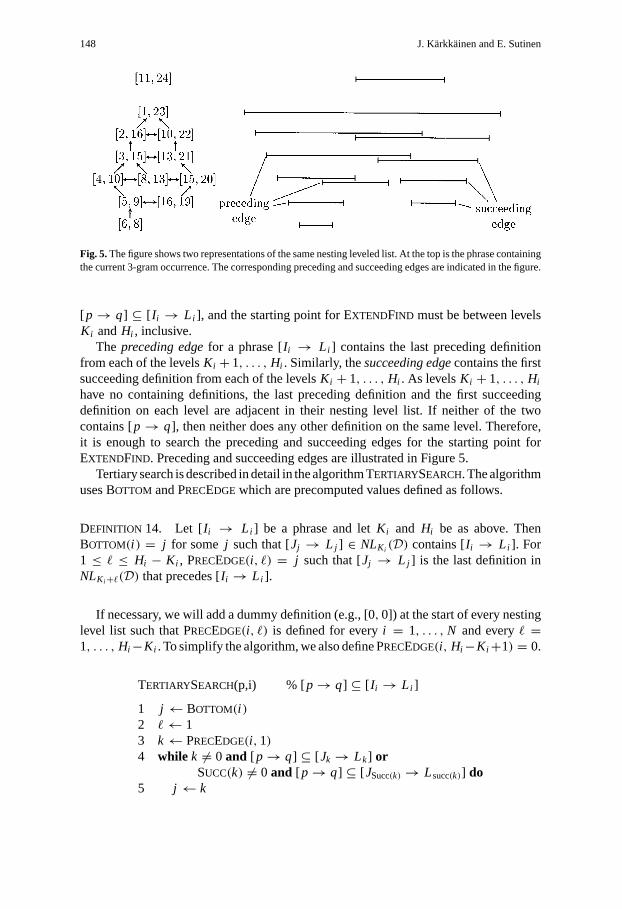
Fig. 5.The figure shows two representations of the same nesting leveled list. At the top is the phrase containingthe current 3-gram occurrence. The corresponding preceding and succeeding edges are indicated in the figure.
[ p→ q] ⊆ [ Ii → Li ], and the starting point for EXTENDFIND must be between levelsKi andHi , inclusive.
The preceding edgefor a phrase [Ii → Li ] contains the last preceding definitionfrom each of the levelsKi + 1, . . . , Hi . Similarly, thesucceeding edgecontains the firstsucceeding definition from each of the levelsKi + 1, . . . , Hi . As levelsKi + 1, . . . , Hi
have no containing definitions, the last preceding definition and the first succeedingdefinition on each level are adjacent in their nesting level list. If neither of the twocontains [p→ q], then neither does any other definition on the same level. Therefore,it is enough to search the preceding and succeeding edges for the starting point forEXTENDFIND. Preceding and succeeding edges are illustrated in Figure 5.
Tertiary search is described in detail in the algorithm TERTIARYSEARCH. The algorithmuses BOTTOM and PRECEDGE which are precomputed values defined as follows.
DEFINITION 14. Let [Ii → Li ] be a phrase and letKi and Hi be as above. ThenBOTTOM(i ) = j for some j such that [Jj → L j ] ∈ NLKi (D) contains [Ii → Li ]. For1 ≤ ` ≤ Hi − Ki , PRECEDGE(i, `) = j such that [Jj → L j ] is the last definition inNLKi+`(D) that precedes [Ii → Li ].
If necessary, we will add a dummy definition (e.g., [0, 0]) at the start of every nestinglevel list such that PRECEDGE(i, `) is defined for everyi = 1, . . . , N and every =1, . . . , Hi−Ki . To simplify the algorithm, we also define PRECEDGE(i, Hi−Ki+1) = 0.
TERTIARYSEARCH(p,i) % [p→ q] ⊆ [ Ii → Li ]
1 j ← BOTTOM(i )2 `← 13 k← PRECEDGE(i, 1)4 while k 6= 0 and [ p→ q] ⊆ [ Jk → Lk] or
SUCC(k) 6= 0 and [ p→ q] ⊆ [ JSucc(k)→ Lsucc(k)] do5 j ← k
Lempel–Ziv Index forq-Grams 149
6 `← `+ 17 k← PRECEDGE(i, `)8 if j = 0 then return ∅9 else
10 if [ p→ q] * [ Jj → L j ] then j ← SUCC( j )11 return EXTENDFIND( j, p)
Each round of thewhile loop in TERTIARYSEARCH passes a definition that contains[ p→ q]. Each of those definitions will be found and returned by EXTENDFIND and willlead to a discovery of a new occurrence. Therefore, the whole tertiary search runs in timelinear in the number of occurrences found.
The space requirement for the BOTTOM pointers is clearlyO(N). For each valuePRECEDGE(i, `), there is at least one preceding or succeeding definition that overlaps[ Ii → Li ] by at leastq positions. By Fact 2(i), phrases cannot overlap each other by morethanq− 1 positions. Thus, a definition may overlap at most two phrases byq positionswithout containing them. Therefore, the total space requirement of the PRECEDGEvaluesis O(N).
7. Construction. The construction of the LZ index starts by LZ parsing the text usingAlgorithm LZPARSE. Then the primary index and the data structures used in the secondaryand tertiary search are built from the LZ parse and the first occurrences ofq-grams. Wenext sketch an algorithm that constructs all the secondary and tertiary search structures:the nesting leveled list, and the START, BOTTOM, and PRECEDGE pointers.
The LZ parsing outputs three kinds of intervals: phrases, definitions andq-gramoccurrences. The secondary and tertiary index construction starts by sorting all theseintervals together by the starting position. The intervals are then processed in the sortedorder:
• When a definition is encountered, it is added to the (originally empty) nesting leveledlist NLL.• When an occurrence [Pi → q] is encountered, the value START(i ) is computed.• When a phrase [Ii → Li ] is encountered, BOTTOM(i ) and PRECEDGE(i, `), for 1 ≤` ≤ Hi − Ki , are computed.
A more detailed description of the construction algorithm is given below:
1. All three kinds of intervals are sorted together into increasing order of the startingpositions. Among intervals with the same starting position, definitions are placedbefore occurrences and phrases, and the length (or end position) is used as an addi-tional key if necessary. The sorting can be done inO(n) time and space using radixsorting.
2. The intervals are processed in the sorted order. Let [I , J] be the interval to be processednext and letK be the deepest level in the current NLL that has a definition [Jj → L j ]containing [I , J]. The levelK and the definition [Jj → L j ] are found by a binarysearch among the latest definitions of the nesting levels. Over the whole algorithmthis takesO(N log H) time, whereH is the depth of the NLL.
150 J. Karkkainen and E. Sutinen
3. The rest of the processing of the interval [I , J] depends on its type:(a) Let [I , J] be the definition [Ji → Li ]. If [ Ji → Li ] ≺ [ Jj → L j ], then add
[ Ji → Li ] into NLL as the last definition on levelK + 1 and set PARENT(i ) = j .Otherwise (i.e., whenJi + Li = Jj + L j ) add [Ji → Li ] into NLL as the lastdefinition on levelK and set PARENT(i ) = PARENT( j ).
In the former case, [Ji → Li ] may belong to the succeeding edge of the latestphrase [Ik → Lk]. Following Section 6, letKk and Hk be such that the currentPRECEDGElist for [ Ik → Lk] is from levelKk+1 toHk. If Hk = K and [Ji → Li ]overlaps [Ik → Lk] by at leastq characters, then set PRECEDGE(k, K+1−Kk) =PREC(i ). If PREC(i ) = 0 (i.e., [Ji → Li ] is the first definition on levelK + 1),add a dummy definition at the start of levelK + 1.
(b) If [ I , J] is the occurrence [Pi → q], set START(i ) = j .(c) If [ I , J] is the phrase [Ii → Li ], set BOTTOM(i ) = j . Additionally, for ` =
1, 2, . . ., set PRECEDGE(i, `) = k, where [Jk → Lk] is the currently last definitionon level K + `, until [Jk → Lk] no longer overlaps [Ii → Li ] by at leastqpositions.
In total, the construction works inO(n+ N log H) time andO(n) space. The depthH of the NLL is clearly at mostN, giving O(n + N log N) construction time. WhenN = O(n/logn) (see the next section), the construction time isO(n). It can also beshown thatH <
√n. In practice,H is still much smaller.
8. The Size of the LZ Index. The primary index of our method can be implementedin O(M) space, whereM is the number of distinctq-grams in the text. The secondaryand tertiary indexes requireO(N) space, whereN is the number of phrases in the LZparse of the text. The total space requirement is thereforeO(M + N). In the followingwe show that this can be sublinear (see [9]). All analysis below assumes that the size ofthe alphabet is constant.
LEMMA 15. The number of phrases of length at most` ≥ q is at most(c`−q+1− 1)M ,where c is the size of the alphabet.
PROOF. Consider the noncoveredq-gram occurrences and the phrases of length at most`, all extended from the end up to length`+1. Due to the properties of Algorithm 1, eachsuch extended interval must be the first occurrence of the corresponding substring and,therefore, the extended intervals all have different content. Each extended interval startswith one of theM distinctq-grams appearing in the text followed by`−q+1 characters.Thus, there can be at mostc`−q+1M extended intervals, of whichM are extensions ofnoncovered occurrences.
LEMMA 16. Let k= dlogc((M + N)/M)e. Then the length of the text is
n >
(k− c
c− 1
)(M + N)+ M + q − 1.
PROOF. If there are no phrases (i.e.,N = 0, k = 0), n = M + q − 1. Otherwise,each phrase overlaps the preceding phrase or noncoveredq-gram occurrence byq − 1
Lempel–Ziv Index forq-Grams 151
characters and, therefore, a phrase of lengthl addsl − q + 1 to the length of the text.Lemma 15 limits the number of short phrases. Specifically, withk such that(ck−1 −1)M < N ≤ (ck − 1)M , there must be phrases of length at leastk + q − 1. Fromfurther application of Lemma 15, we can then deduce thatN phrases add at leastkN−M∑k−1
i=0(ci − 1) to the length of the text. Therefore,
n ≥ M + q − 1+ kN− Mk−1∑i=0
(ci − 1) = k(M + N)− Mk−1∑i=0
ci + M + q − 1.
The result follows when we note thatk−1∑i=0
ci = ck − 1
c− 1<
c
c− 1
M + N
M.
THEOREM17. If M = O(n/( f (n) log f (n))), for f (n) such that f(n) log f (n) =O(n) and f(n) = Ä(1), then N= O(n/log f (n)).
PROOF. If N = Ä(n/log f (n)), thenk = Ä(log f (n)) and, by Lemma 16,
N <n− M − q + 1
k− c/(c− 1)− M = O
(n
log f (n)
).
COROLLARY 18. If M = O(n1−ε),whereε is a positive constant, then N= O(n/logn).
PROOF. Choosef (n) = nε/logn in Theorem 17.
COROLLARY 19. If q ≤ (1− ε) log|6| n+ C, whereε is a positive constant and C isan arbitrary constant, then M+ N = O(n/logn).
The sublinearity conditions of Theorem 17, Corollary 18, and Corollary 19 are suf-ficient but not necessary. For a compressible text, the LZ index can have sublinear sizeeven if the conditions are not satisfied.
As is customary, the sizes refer to the number of words needed to store the datastructure given the assumption that a word can store an arbitrary pointer. However, apointer to the text, for example, needs at least logn bits. Thus, measured in bits, bytes,or other constant units, the size of the LZ index under the conditions of Corollary 18is actuallyO(n) and the size of a traditionalq-gram index isO(n logn). On the otherhand, the text itself could be packed inO(n/logn) words of sizeÄ(logn). Therefore,let ||T || denote thesize(in contrast to the length) of the text in whichever space unitsare being used. Then the size of the LZ index isO(||T ||), while the size of a traditionalq-gram index isO(||T || log||T ||).
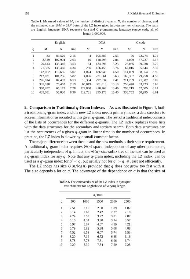
Table 1 shows measured values ofM andN, and an estimated size of the LZ index forsome texts. The actual size of the data structures depends on the implementation and mayalso depend on other statistics besidesM andN (e.g., the shape of the primary index trieand the number of PRECEDGE-values). However, the estimate 16M +24N bytes used inTable 1 should be fairly close to an average size of a reasonable implementation. Table 2shows the estimated size as the text length increases.
152 J. Karkkainen and E. Sutinen
Table 1. Measured values ofM , the number of distinctq-grams,N, the number of phrases, andthe estimated size 16M + 24N bytes of the LZ index given in bytes per text character. The textsare English language, DNA sequence data and C programming language source code, all of
9. Comparison to Traditional q-Gram Indexes. As was illustrated in Figure 1, botha traditionalq-gram index and the new LZ index need a primary index, a data structure toaccess information associated with a givenq-gram. The rest of a traditional index consistsof the lists of occurrences for the differentq-grams. The LZ index replaces these listswith the data structures for the secondary and tertiary search. Both data structures canlist the occurrences of a givenq-gram in linear time in the number of occurrences. Inpractice, the LZ index is slower by a small constant factor.
The major difference between the old and the new methods is their space requirement.A traditionalq-gram index requires2(n) space, independent of any other parameters,particularly independent ofq. In fact, the2(n)-size suffix tree of the text can be used asa q-gram index for anyq. Note that anyq-gram index, including the LZ index, can beused as aq′-gram index forq′ < q, but usually not forq′ > q, at least not efficiently.
The LZ index has sizeO(n/logn) provided thatq does not grow too fast withn.The size depends a lot onq. The advantage of the dependence onq is that the size of
Table 2.The estimated size of the LZ index in bytes pertext character for English text of varying length.
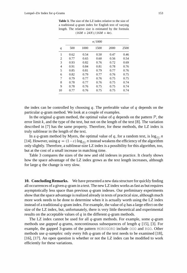
Table 3.The size of the LZ index relative to the size ofa traditionalq-gram index for English text of varyinglength. The relative size is estimated by the formula
the index can be controlled by choosingq. The preferable value ofq depends on theparticularq-gram method. We look at a couple of examples.
In the originalq-gram method, the optimal value ofq depends on the patternP, theerror limit k, and the type of the text, but not on the length of the text [8]. The variationdescribed in [7] has the same property. Therefore, for these methods, the LZ index istruly sublinear in the length of the text.
In a q-gram method by Myers, the optimal value ofq, for a random text, is log|6| n[14]. However, usingq = (1−ε) log|6| n instead weakens the efficiency of the algorithmonly slightly. Therefore, a sublinear-size LZ index is a possibility for this algorithm, too,but at the cost of a small increase in matching time.
Table 3 compares the sizes of the new and old indexes in practice. It clearly showshow the space advantage of the LZ index grows as the text length increases, althoughfor largeq the change is very slow.
10. Concluding Remarks. We have presented a new data structure for quickly findingall occurrences of a givenq-gram in a text. The new LZ index works as fast as but requiresasymptotically less space than previousq-gram indexes. Our preliminary experimentsshow that the space advantage is realized already in texts of practical size, although muchmore work needs to be done to determine when it is actually worth using the LZ indexinstead of a traditionalq-gram index. For example, the value ofq has a large effect on thesize of the LZ index, but, unfortunately, there is very little theoretical and experimentalresults on the acceptable values ofq in the differentq-gram methods.
The LZ index cannot be used for allq-gram methods. For example, someq-grammethods usegapped q-grams, noncontinuous subsequences of lengthq [15], [3]. Forexample, the gapped 3-grams of the patternMOROGOROincludeOOOandRGO. Othermethods useq-samples: only everyhth q-gram of the text needs to be examined [18],[16], [17]. An open question is whether or not the LZ index can be modified to workefficiently for these variations.
154 J. Karkkainen and E. Sutinen
References
[1] R. Baeza-Yates: Space–time trade-offs in text retrieval. In:Proc. First South American Workshop onString Processing(eds. R. Baeza-Yates and N. Ziviani), Universidade Federal de Minas Gerais, 1993,pp. 15–21.
[2] R. Boyer and S. Moore: A fast string searching algorithm.Comm. ACM 20(10) (1977), 762–772.[3] A. Califano and I. Rigoutsos: FLASH: A fast look-up algorithm for string homology. In:Proc. First
International Conference on Intelligent Systems for Molecular Biology(eds. L. Hunter, D. Searls, andJ. Shavlik), AAAI Press, Menlo Park, 1993, pp. 56–64.
[4] W. Chang and E. Lawler: Sublinear approximate string matching and biological applications.Algorith-mica12 (4–5) (1994), 327–344.
[5] W. Chang and T. Marr: Approximate string matching and local similarity. In:Proc. 5th Annual Sym-posium on Combinatorial Pattern Matching CPM ’94 (eds. M. Crochemore and D. Gusfield), LectureNotes in Computer Science, Vol. 807, Springer-Verlag, Berlin, 1994, pp. 259–273.
[6] R. Grossi and F. Luccio: Simple and efficient string matching withk mismatches.Inform. Process. Lett.33 (1989), 113–120.
[7] N. Holsti and E. Sutinen: Approximate string matching usingq-gram places. In:Proc. Seventh FinnishSymposium on Computer Science(ed. M. Penttonen), University of Joensuu, 1994, pp. 23–32.
[8] P. Jokinen and E. Ukkonen: Two algorithms for approximate string matching in static texts. In:Proc.Mathematical Foundations of Computer Science1991 (ed. A. Tarlecki), Lecture Notes in ComputerScience, Vol. 520, Springer-Verlag, Berlin, 1991, pp. 240–248.
[9] J. Karkkainen and E. Ukkonen: Lempel–Ziv parsing and sublinear-size index structures for stringmatching. In:Proc. 3rd South American Workshop on String Processing WSP ’96 (eds. N. Ziviani etal.), Carleton University Press, Ottawa, 1996, pp. 141–155.
[10] G. Landau and U. Vishkin: Fast string matching withk differences.J. Comput. System Sci. 37 (1988),63–78.
[11] O. Lehtinen, E. Sutinen, and J. Tarhio: Experiments on block indexing. In:Proc. 3rd South AmericanWorkshop on String Processing WSP ’96 (eds. N. Ziviani et al.), Carleton University Press, Ottawa,1996, pp. 183–193.
[12] A. Lempel and J. Ziv: On the complexity of finite sequences.IEEE Trans. Inform. Theory, 22(1) (1977),75–81.
[13] E. M. McCreight: A space-economical suffix tree construction algorithm.J. Assoc. Comput. Mach. 23(1976), 262–272.
[14] E. Myers: A sublinear algorithm for approximate keyword searching.Algorithmica12(4–5) (1994),345–374.
[15] P. Pevzner and M. Waterman: Multiple filtration and approximate pattern matching.Algorithmica13(1995), 135–154.
[16] E. Sutinen and J. Tarhio: On usingq-gram locations in approximate string matching. In:Proc. 3rdAnnual European Symposium on Algorithms ESA ’95 (ed. P. Spirakis), Lecture Notes in ComputerScience, Vol. 979, Springer-Verlag, Berlin, 1995, pp. 327–340.
[17] E. Sutinen and J. Tarhio: Filtration withq-samples in approximate string matching. In:Proc. 7thSymposium on Combinatorial Pattern Matching CPM ’96 (ed. D. Hirschberg and G. Myers), LectureNotes in Computer Science, Vol. 1075, Springer-Verlag, Berlin, 1996, pp. 50–63.
[18] T. Takaoka: Approximate pattern matching with samples. In:Proc. 5th Symposium on Algorithms andComputation ISAAC ’94, Lecture Notes in Computer Science, Vol. 834, Springer-Verlag, Berlin, 1994,pp. 234–242.
[19] J. Tarhio and E. Ukkonen: Approximate Boyer-Moore string matching.SIAM J. Comput. 22(2) (1993),243–260.
[20] E. Ukkonen: Finding approximate patterns in strings.J. Algorithms6 (1985), 132–137.[21] E. Ukkonen: Approximate string matching withq-grams and maximal matches.Theoret. Comput. Sci.
92(1) (1992), 191–211.[22] E. Ukkonen: On-line construction of suffix-trees.Algorithmica14 (1995), 249–260.[23] S. Wu and U. Manber: Fast text searching allowing errors.Comm. ACM 35(10) (1992), 83–91.[24] J. Ziv and A. Lempel: A universal algorithm for sequential data compression.IEEE Trans. Inform.