Lesson 12Magnetostatics in Materials

楊尚達 Shang-Da YangInstitute of Photonics TechnologiesDepartment of Electrical EngineeringNational Tsing Hua University, Taiwan

Outline

Static magnetic field in materialsBoundary conditionsProperties of magnetic materials

Sec. 12-1Static Magnetic Field in Materials

1. Classical models of induced magnetic dipoles

2. Magnetization vectors3. Magnetization currents4. Magnetic field intensities

Induced magnetic dipole-1

Any material has many small magnetic dipoles (current loops) arising from (1) orbiting electrons, (2) spinning nucleus and electrons

A material bulk made up of a large number of randomly oriented molecules typically has no macroscopic dipole moment in the absence of external magnetic field

What’s spin? (1)

Spin of elementary particles cannot be explained by assuming they are made up of even smaller particles rotating about a center

Spin is about angular momentum of elementary particles, quantized, cannot be altered

What’s spin? (2)

A particle with charge q, mass m, spin S has an intrinsic magnetic dipole moment:

Smqg

2=μ

2≈g

Angular momentum of an electron (spin-1/2) measured along any direction can only take on values of 2h±

Photon (spin-1): h± ,0

Induced magnetic dipole due to orbiting electron-1

00 ωφrau vv =

EeFe

vv−=

204 r

qaE r πεvv

=

rma er20ω

v=

Induced magnetic dipole due to orbiting electron-2

BueFm

vvv×−=

ωφrau vv =

rma er2ωv=

↑==πω

π 22e

rueI

⇒> ,0ωω

( )2rIam z π⋅Δ−=Δ vv

πωω

2)( 0−

=ΔeI

diamagnetism

Induced magnetic dipole due to aligned moment

torque tension

paramagnetism

Strategy of analysis

It is too tedious to directly superpose the elementary fields:

Instead, we define magnetization vector as:

the kth dipole moment inside a differential volume Δv

⇒ Magnetization current , Magnetic field intensity H

v

[ ]θθπμ

θ sincos24

)( 30 aaRmrB R

vvvv +≈

vm

M k

v Δ≡ ∑

→Δ

vv

0lim

mJv

Magnetization surface current density-1

On the air-material interface, is dis-continuous, net magnetization current exists

Mv

Magnetization surface current density-2

Consider a differential volume

with rectangular current loop of

dxdydzV =Δ

,dydzS =Δ I

IdydzaSIaM xxvvv

=Δ=Δ

dxIa

dxdydzIdydza

VMM xx

vvv

v==

ΔΔ

=

Magnetic dipole moment:

Magnetization vector:

Magnetization surface current density-3

By inspection, the surface current density:dx

IaVMM x

vv

v=

ΔΔ

=

⎟⎠⎞

⎜⎝⎛=

mA

dxIaJ zms

vv

( )mA nms aMJ vvv×=⇒

To generalize the result,

,dxIaa

dxIaaM zyxn

vvvvv=×=×

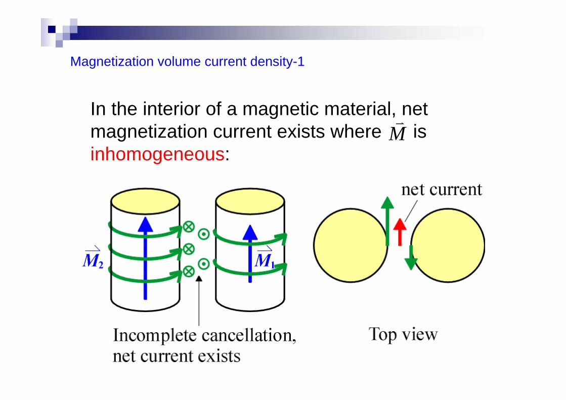
Magnetization volume current density-1

In the interior of a magnetic material, net magnetization current exists where is inhomogeneous:

Mv

Magnetization volume current density-2

Consider two m-dipoles with x-dependent, z-direction magnetization vectors: , )(xMaz

v )( dxxMaz +v

( )

dzxMxIdz

xIdzSSxIxM

)()(

)()(

=⇒

=⋅ΔΔ

=

where

Similarly,

dzdxxMdxxI )()( +=+

Magnetization volume current density-3

Net current passing through the interfacing surface bounded by C is: ( ) ( )

[ ]dzdxxMxMdxxIxI

)()( +−=+−

The current density is:

dxdzdxxIxIaJ ym

)()( +−= v

v

xMa

dxdxxMxMa

zy

y

∂∂

−=

+−=

v

v )()(

Magnetization volume current density-4

xMa

xMx

aaa

MMMzyx

aaaM

zy

z

zyx

zyx

zyx

∂∂

−=∂∂=

∂∂∂∂∂∂=×∇

v

vvv

vvv

v

)(0000

To generalize the result:

( )2mA MJm

vv×∇=⇒

Comment-1

can be regarded as a special case of , where ∞→×∇ M

v

∞→×∇ Mv

nms aMJ vvv×=

MJ m

vv×∇=

vdrrR

rJrAV

′′′

= ∫ ′ 0

),()(

4)( vv

vvvv

πμ

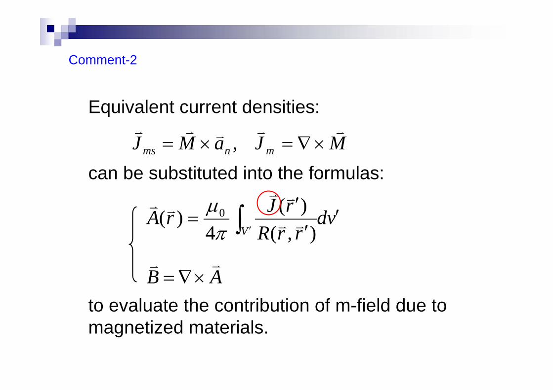
Comment-2

Equivalent current densities:

can be substituted into the formulas:

to evaluate the contribution of m-field due to magnetized materials.

,nms aMJ vvv×= MJ m

vv×∇=

ABvv

×∇=

Example 12-1: Permanent magnet (1)

Consider a uniformly magnetized cylinder of radius b, length L, and . Find the on-axis

0MaM zvv

=

Bv

On the side wall:

00 MaaMaaMJ rznms φvvvvvv

=×=×=

On the top & bottom walls:( ) 00 =±×=×= zznms aMaaMJ vvvvv

In the interior:( ) 00 =×∇=×∇= MaMJ zmvvv

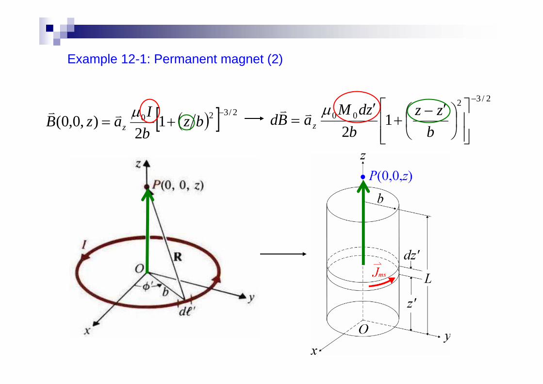
Example 12-1: Permanent magnet (2)

( )[ ] 2/320 12

),0,0(−

+= bzbIazB z

μvv2/32

00 12

−

⎥⎥⎦

⎤

⎢⎢⎣

⎡⎟⎠⎞

⎜⎝⎛ ′−

+′

=b

zzb

zdMaBd z

μvv

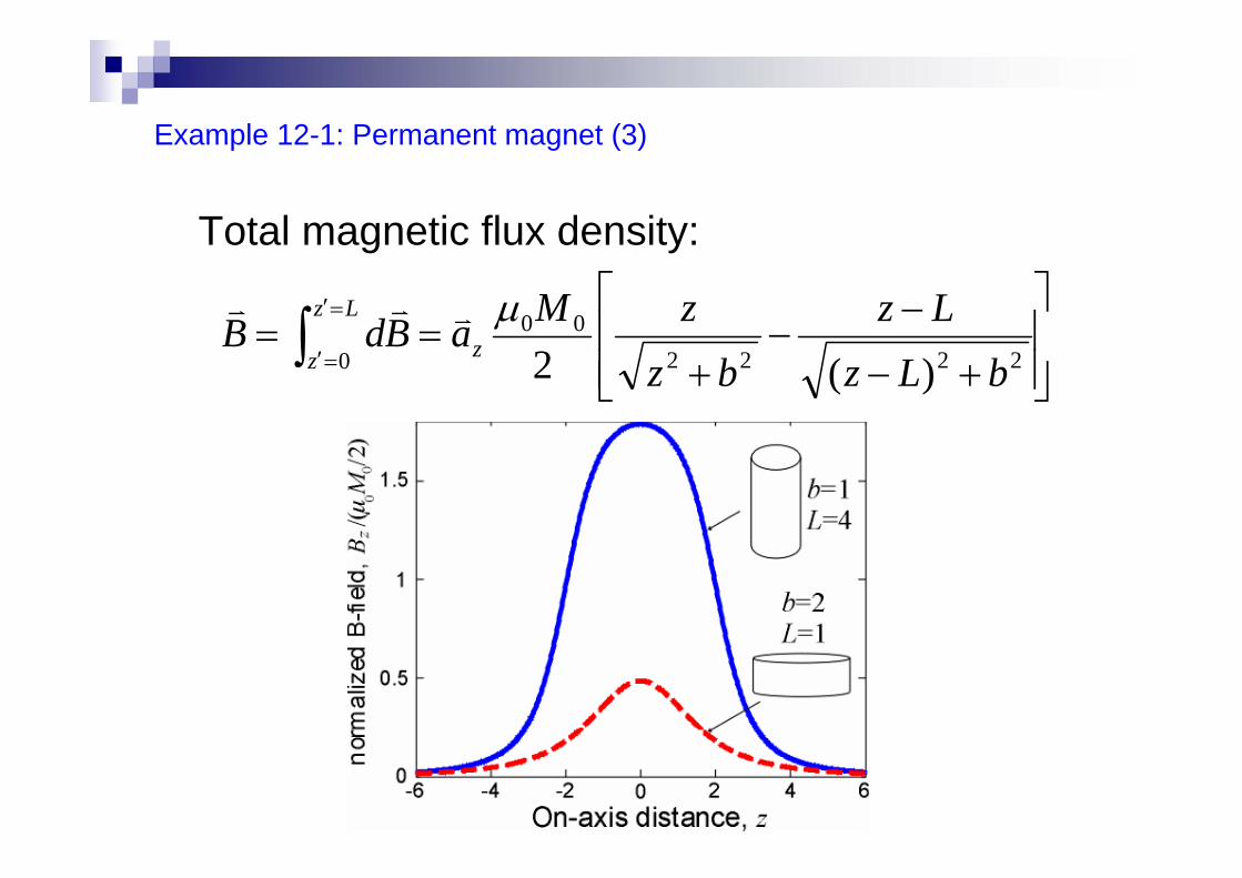
Example 12-1: Permanent magnet (3)

Total magnetic flux density:

⎥⎥⎦

⎤

⎢⎢⎣

⎡

+−

−−

+== ∫

=′

=′ 222200

0 )(2 bLzLz

bzzMaBdB z

Lz

z

μvvv

Magnetic field intensity - Definition (1)

Total M-field is created by free & magnetization currents:

JBrv

0μ=×∇ ( )mJJBvvv

+=×∇ 0μ

Mv

×∇

( ),00 MJBvvv

×∇+=×∇ μμ

( ) ,00 JMBvvv

μμ =×∇−×∇⇒

JMB vvv

=⎟⎟⎠

⎞⎜⎜⎝

⎛−×∇⇒

0μ

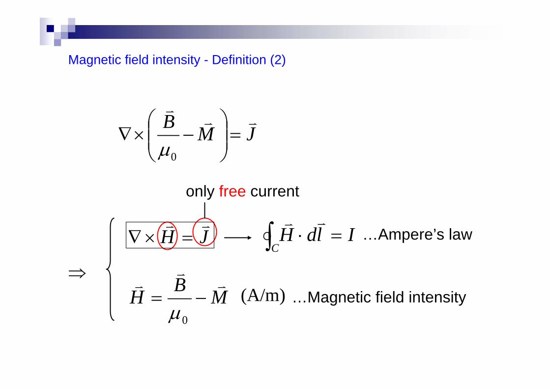
Magnetic field intensity - Definition (2)

⇒(A/m)

…Ampere’s law

only free current

JMB vvv

=⎟⎟⎠

⎞⎜⎜⎝

⎛−×∇

0μ

JHvv

=×∇

MBHv

vv

−=0μ

IldHC

=⋅∫ vv

…Magnetic field intensity

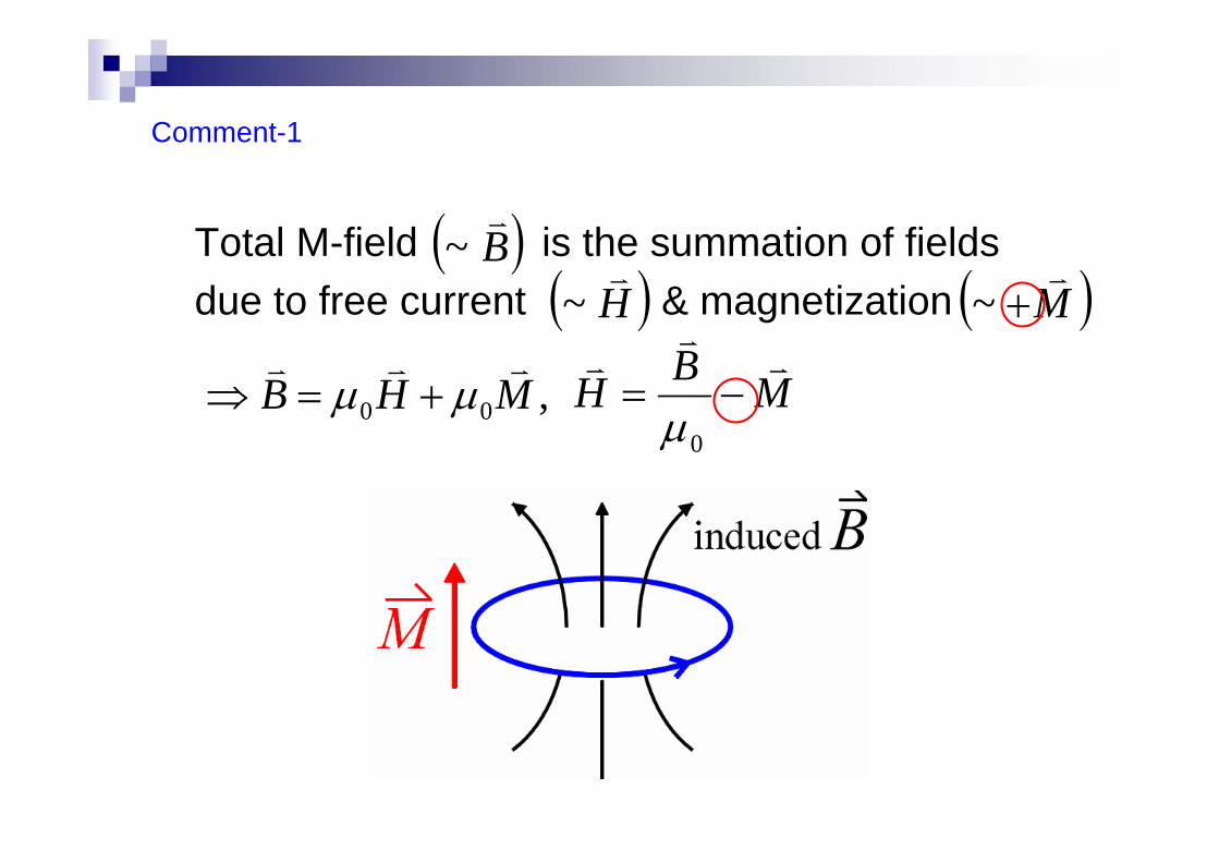
Comment-1

Total M-field is the summation of fields due to free current & magnetization

( )Bv

~( )H

v~ ( )M

v+~

,00 MHBvvv

μμ +=⇒ MBHv

vv

−=0μ

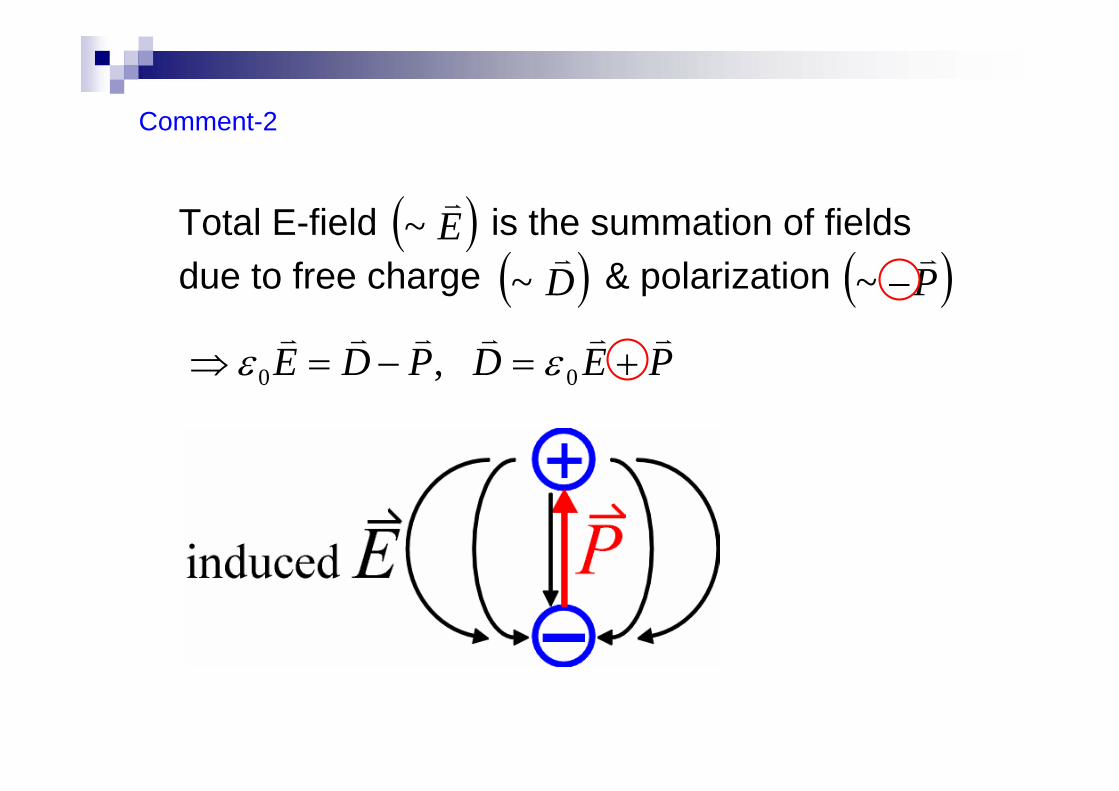
Comment-2

Total E-field is the summation of fields due to free charge & polarization

( )Ev

~( )D

v~ ( )P

v−~

,0 PDEvvv

−=⇒ ε PEDvvv

+= 0ε

0=Hv

0HhHvv

=02HhH

vv=

Magnetic field intensity - Usefulness (1)

For linear, homogeneous, and isotropicmagnetic materials, the magnetization vector is proportional to the external magnetic field :

SIhm ⋅Δ−=vv0=mv

Susceptibility, independent of magnitude, position, and direction of H

vHM m

vvχ=

SIhm ⋅Δ−= 2vv

Magnetic field intensity - Usefulness (2)

⇒

…Permeability of the medium

A single constant replaces the tedious induced m-dipoles, magnetization vector, equivalent magnetization currents in determining the total magnetic field.

μ

,0

MBHv

vv

−=μ

( )MHBvvv

+=⇒ 0μ

( ) ( )HHH mm

vvvχμχμ +=+= 100

HBvv

μ=

( )mχμμ += 10

Example 12-2: Physical meanings of H, M, B

: free current: magnetization current

: total current

Hv

Mv

0μBv

Example 12-3: Magnetic circuit (1)

A current I0 flows in N turns of wire wound around a toroidal core of permeability μ, mean radius r0, cross-sectional radius a, narrow air gap of length lg. Find , both in the core and the air gap.

Bv

Hv

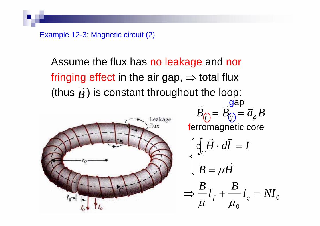
Example 12-3: Magnetic circuit (2)

Assume the flux has no leakage and nor fringing effect in the air gap, ⇒ total flux (thus ) is constant throughout the loop: B

v

BaBB gf φvvv

==

IldHC

=⋅∫ vv

HBvv

μ=

00

NIlBlBgf =+⇒

μμ

ferromagnetic core

gap

Example 12-3: Magnetic circuit (3)

,00

NIlBlBgf =+

μμ 0

0

μμ gf llNIB+

=⇒

,μ

ff

BH

vv

=⇒0μg

g

BH

vv

=

gf BB =

,0μμ >>Q gf HH <<⇒

A small can induce a strong in the ferromagnetic material, providing a majority of magnetic flux in the ferromagnetic core.

fH Mv

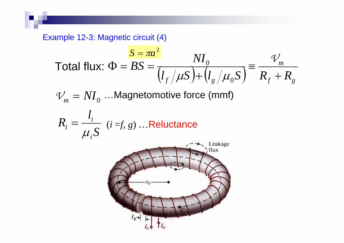
Example 12-3: Magnetic circuit (4)

( ) ( ) gf

m

gf RRSlSlNIBS

+≡

+==Φ

V

0

0

μμTotal flux:

2aS π=

0NIm =V …Magnetomotive force (mmf)

SlRi

ii μ= (i =f, g) …Reluctance

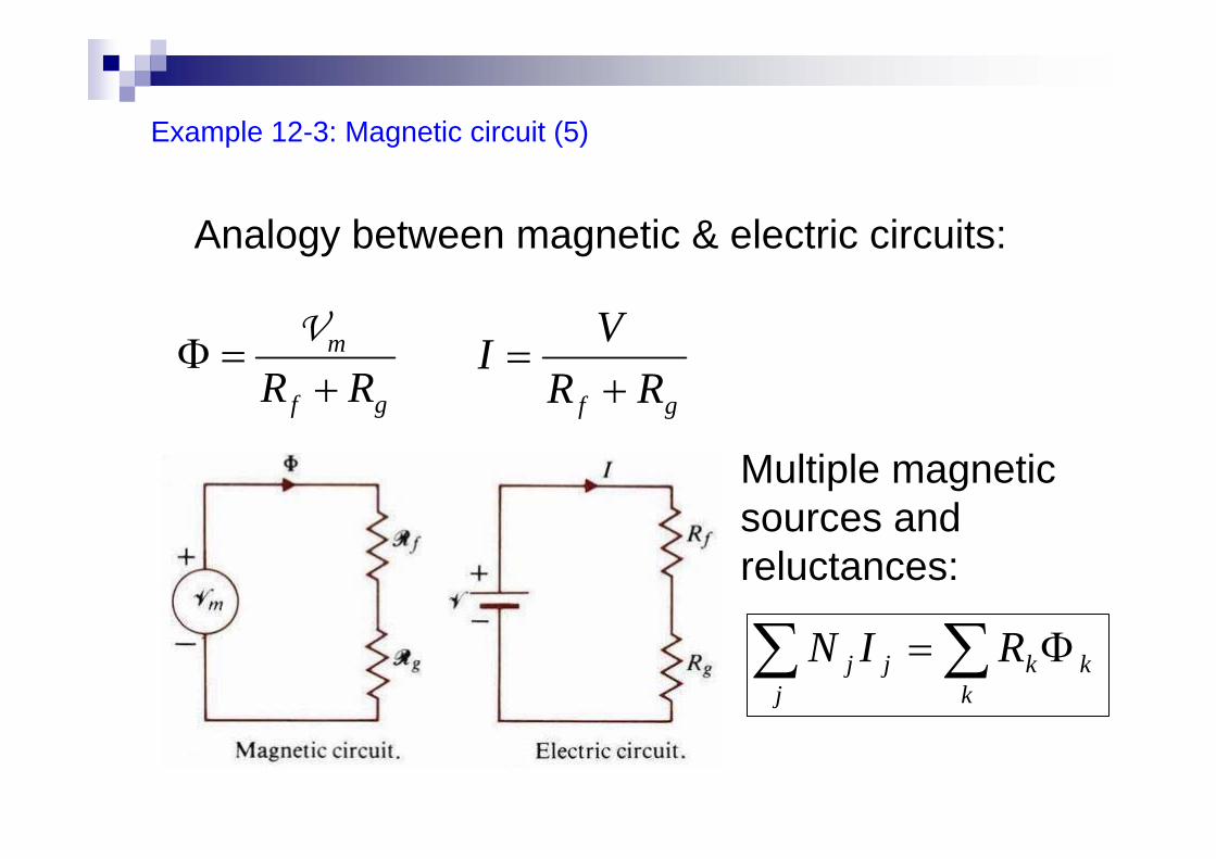
Example 12-3: Magnetic circuit (5)

gf

m

RR +=Φ

V

Analogy between magnetic & electric circuits:

gf RRVI+

=

∑∑ Φ=k

kkj

jj RIN

Multiple magnetic sources and reluctances:

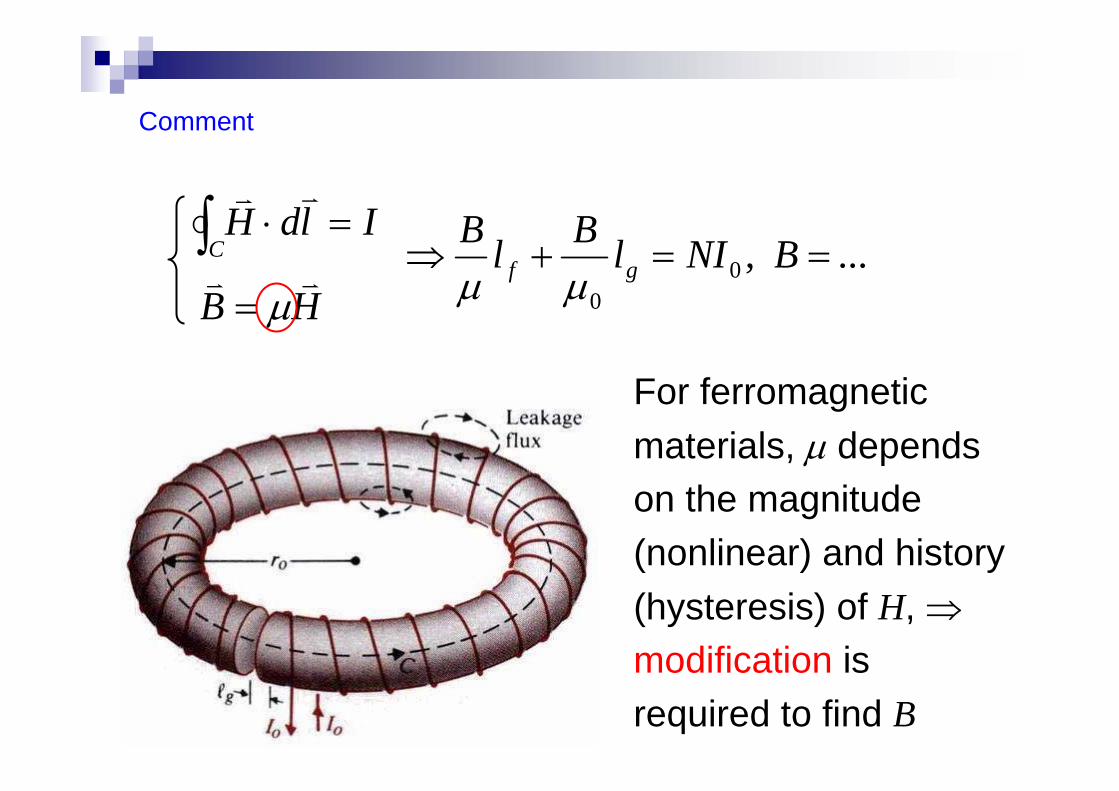
Comment

IldHC

=⋅∫ vv

HBvv

μ=... ,0

0

==+⇒ BNIlBlBgf μμ

For ferromagnetic materials, μ depends on the magnitude (nonlinear) and history (hysteresis) of H, ⇒modification is required to find B

Sec. 12-2Boundary Conditions

1. Tangential boundary condition2. Normal boundary condition

Tangential BC-1

⇒

,

IldHC

=⋅∫vv

)( 21 wHwHldH

abcda

vvvvvvΔ−⋅+Δ⋅=⋅⇒ ∫

wJwHwH sntt Δ=Δ⋅−Δ⋅= 21

sntt JHH =− 21

Component of in the ab-direction

iHv

In general,

( ) sn JHHavvvv =−× 212

Component of along thumbav

sJv

Comment

The projections of and on the interface are generally not collinear.

1Hv

2Hv

( ) sn JHHavvvv =−× 212,21 sntt JHH =−

Normal BC-1

⇒

,0

=⋅∫SsdB vv ( )( ) 0 2221

=Δ⋅−⋅=⋅⇒ ∫ SaBaBsdB nnS

vvvvvv

nn BB 21 =

Comment-1

Only free surface current density counts in:

If the two interfacing media are non-conducting:

( ) sn JHHavvvv =−× 212

tts HHJ 21 ,0 =⇒=v

Comment-2

remain valid even the M-fields are time-varying.

( ) sn JHHavvvv =−× 212

nn BB 21 =

Comment-3

tt EE 21 =

( ) sn DDa ρ=−⋅ 212

vvv

( ) sn JHHavvvv =−× 212

nn BB 21 =v.s.

BCs in electrostatics: BCs in magnetostatics:

Sec. 12-3Properties of Magnetic Materials

1. Diamagnetic materials2. Paramagnetic materials3. Quantum view of ferromagnetism4. Hysteresis curve

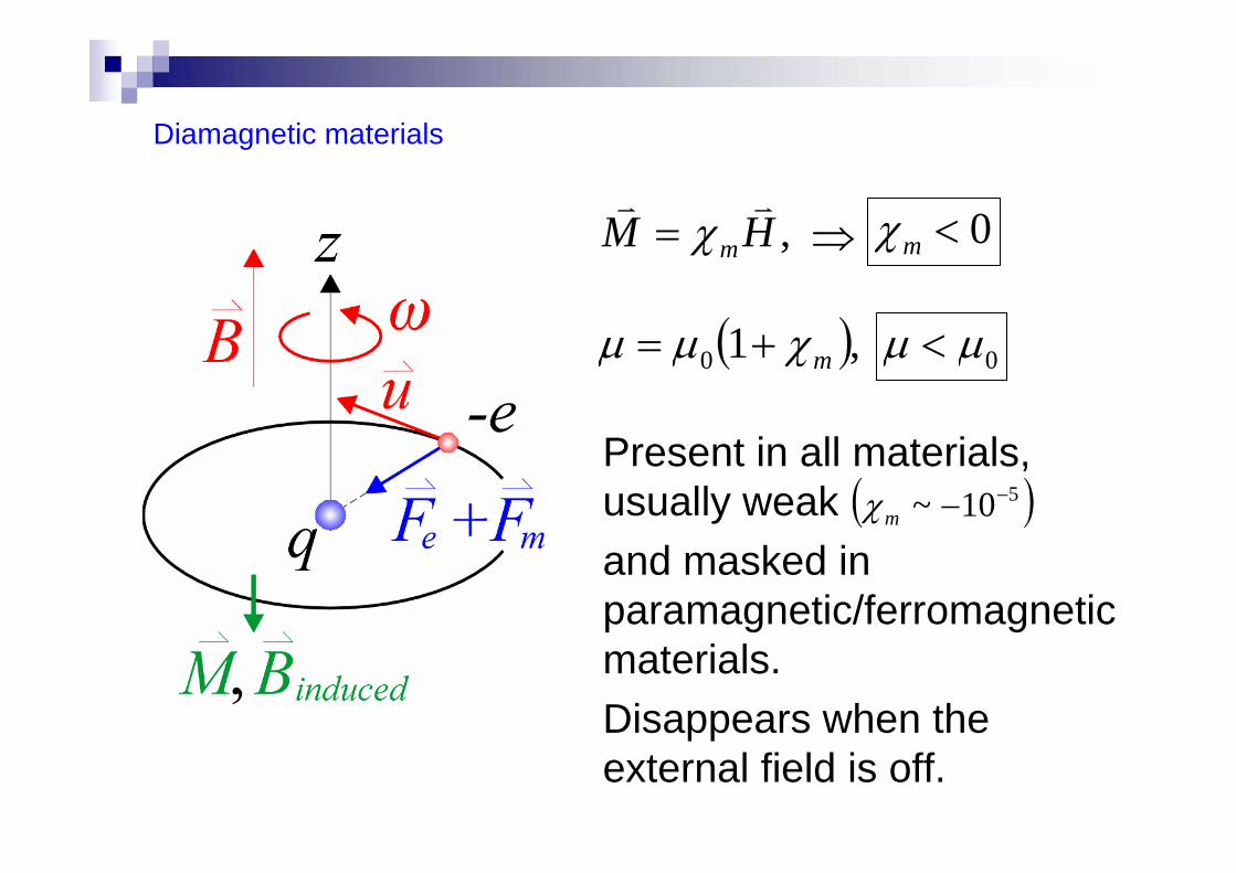
Diamagnetic materials

,HM m

vvχ= 0<mχ

( ),10 mχμμ += 0μμ <

⇒

Present in all materials, usually weakand masked in paramagnetic/ferromagnetic materials. Disappears when the external field is off.

( )510~ −−mχ

Diamagnetic materials-examples

pyrolytic graphite

permanent neodymium magnet

Frog flying in strong M-field(D=32 mm, B=16T)

Paramagnetic materials

,HM m

vvχ= 0>mχ

( ),10 mχμμ += 0μμ >

⇒

( )510~ −mχUsually very weak

reduced by thermal vibration (randomizing the dipole moments). Disappears when the external field is off.

Ferromagnetic materials-1

Non-classical, can only be explained by quantum mechanical view.

Ferromagnetism is determined by both the chemical makeup and the crystalline structure. E.g.

1. Heusler alloys: ferromagnetic, but constituents are not ferromagnetic.

2. Stainless steel: not ferromagnetic, but composed almost exclusively of ferromagnetic metals.

Ferromagnetic materials-2

Main source: the spin of the electrons, Pauli’sexclusion principle (quantum mechanical).

For atoms with fully filled shell (electrons are paired with up/down spins), no net dipole moment exists.

Ferromagnetic materials-3

For atoms with partially filled shell (unpairedelectrons/spins exist), net dipole moment arise.

E.g. Lanthanide elements can carry up to 7 unpaired electrons in the 4f-orbitals

Quantum numbers:n =1, 2, .., ~energy

l =0(s), 1(p), 2(d), 3(f), ..(n-1), .., ~angular momentum, orbital shape, # of nodal planes

ml = -l, …, l, ~axis

ms = 1/2, -1/2, ~spin

Ferromagnetic materials-4

Unpaired dipoles tend to align in parallel to external M-field (classical model), ⇒paramagnetism

Unpaired dipoles tend to align spontaneously, (quantum mechanical effect), ⇒ferromagnetism

Ferromagnetic materials-5

Exchange interaction:

Two electrons (fermions) from adjacent atoms with parallel spins will have lower system energy (more stable) than those with opposite spins.

021 <⋅− SJS

Energy difference due to spin-spin interaction:

>0, if parallel spins>0, if pure Coulomb interaction

Ferromagnetic materials-6

In iron, exchange (spin-spin) interaction is 1000 times stronger than dipole-dipole interaction, ⇒spontaneous alignment, magnetic domains.

At long distance, exchange interaction is overtaken by tendency of dipoles to anti-align, ⇒many randomly oriented domains.

Ferromagnetic materials-7

Placed in strong external M-field, domains will be aligned with the field.

The alignment remains after the field is turned off because the domain walls are pinned on defects in the lattice, ⇒ permanent magnets.

Domains are disorganized (demagnetized) if above Curie temperature (thermal energy > exchange interaction energy).

Hysteresis curve-1

1. Reversible magnetization: if external M-field is weak (up to P1), domain wall movement is reversible, ⇒ B-H curve is a function

Hysteresis curve-2

2. Hysteresis: If external M-field is changed from H2 to H'2, B will change along the upper branch (from P2 to P'2). Conversely, along lower branch.

3. Saturation: If the external field is very strong (above P3), all the domains are aligned.