Page 129 Lesson 4 – Linear Functions and Applications In this lesson, we take a close look at Linear Functions and how real world situations can be modeled using Linear Functions. We study the relationship between Average Rate of Change and Slope and how to interpret these characteristics. We also learn how to create Linear Models for data sets using Linear Regression. Lesson Topics: Section 4.1: Review of Linear Functions Section 4.2: Average Rate of Change Average Rate of Change as slope Interpret the Average Rate of Change Use the Average Rate of Change to determine if a function is Linear Section 4.3: Scatterplots on the Graphing Calculator Section 4.4: Linear Regression Using your graphing calculator to generate a Linear Regression equation Using Linear Regression to solve application problems Section 4.5: Multiple Ways to Determine the Equation of a Line
Transcript
Page 129
Lesson 4 – Linear Functions and Applications In this lesson, we take a close look at Linear Functions and how real world situations can be modeled using Linear Functions. We study the relationship between Average Rate of Change and Slope and how to interpret these characteristics. We also learn how to create Linear Models for data sets using Linear Regression. Lesson Topics: Section 4.1: Review of Linear Functions Section 4.2: Average Rate of Change
§ Average Rate of Change as slope § Interpret the Average Rate of Change § Use the Average Rate of Change to determine if a function is Linear
Section 4.3: Scatterplots on the Graphing Calculator
Section 4.4: Linear Regression
§ Using your graphing calculator to generate a Linear Regression equation § Using Linear Regression to solve application problems
Section 4.5: Multiple Ways to Determine the Equation of a Line
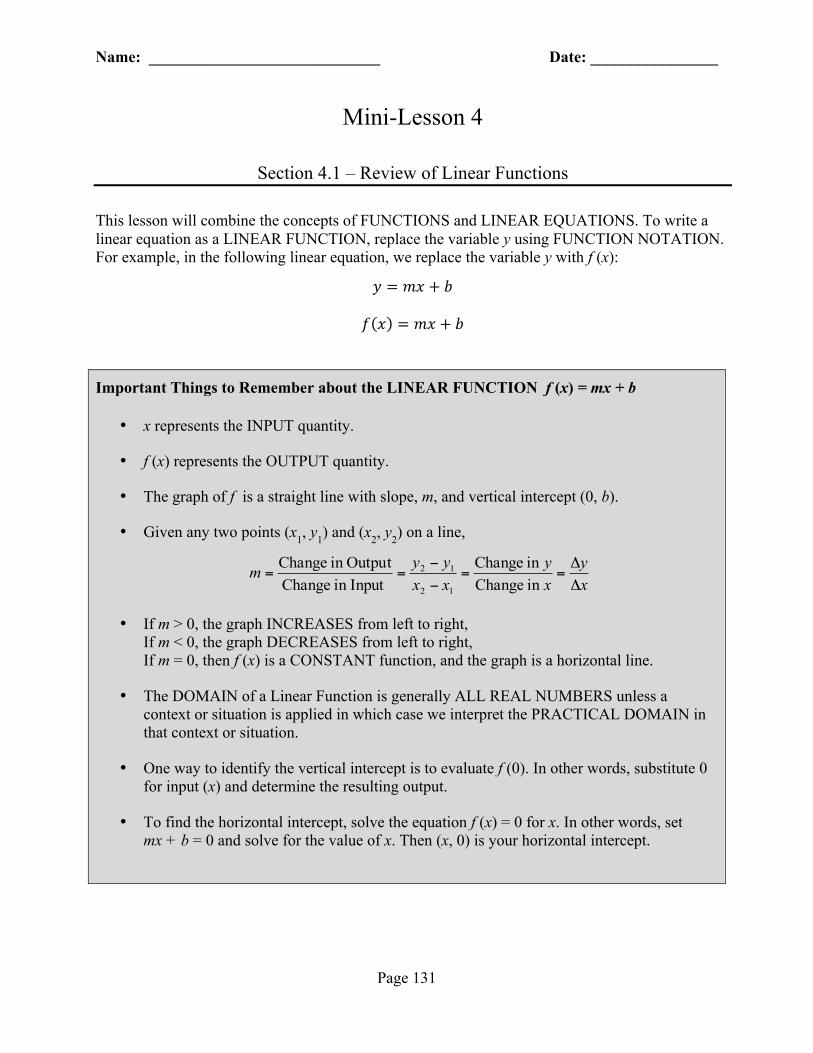
Section 4.1 – Review of Linear Functions This lesson will combine the concepts of FUNCTIONS and LINEAR EQUATIONS. To write a linear equation as a LINEAR FUNCTION, replace the variable y using FUNCTION NOTATION. For example, in the following linear equation, we replace the variable y with f (x):
! = !" + !
! ! = !" + !
Important Things to Remember about the LINEAR FUNCTION f (x) = mx + b
• x represents the INPUT quantity.
• f (x) represents the OUTPUT quantity.
• The graph of f is a straight line with slope, m, and vertical intercept (0, b).
• Given any two points (x1, y1) and (x2, y2) on a line,
xy
xy
xxyym
ΔΔ
==−
−==
in Changein Change
Input in ChangeOutputin Change
12
12
• If m > 0, the graph INCREASES from left to right, If m < 0, the graph DECREASES from left to right, If m = 0, then f (x) is a CONSTANT function, and the graph is a horizontal line.
• The DOMAIN of a Linear Function is generally ALL REAL NUMBERS unless a context or situation is applied in which case we interpret the PRACTICAL DOMAIN in that context or situation.
• One way to identify the vertical intercept is to evaluate f (0). In other words, substitute 0 for input (x) and determine the resulting output.
• To find the horizontal intercept, solve the equation f (x) = 0 for x. In other words, set mx + b = 0 and solve for the value of x. Then (x, 0) is your horizontal intercept.
Lesson 4 – Linear Functions and Applications Mini-Lesson
Page 132
Problem 1 YOU TRY – Review of Linear Functions The function E(t) = 3861 – 77.2t gives the surface elevation (in feet above sea level) of Lake Powell t years after 1999. a) Identify the vertical intercept of this linear function and write a sentence explaining its meaning in this situation. b) Determine the surface elevation of Lake Powell in the year 2001. Show your work, and write your answer in a complete sentence. c) Determine E(4), and write a sentence explaining the meaning of your answer. d) Is the surface elevation of Lake Powell increasing or decreasing? How do you know? e) This function accurately models the surface elevation of Lake Powell from 1999 to 2005.
Determine the practical range of this linear function.
Lesson 4 – Linear Functions and Applications Mini-Lesson
Page 133
Section 4.2 – Average Rate of Change
Average rate of change of a function over a specified interval is the ratio:
xy
xy
Δ
Δ===
in Changein Change
Inputin ChangeOutputin Change Change of Rate Average
Units for the Average Rate of Change are always , unitinput unitsoutput
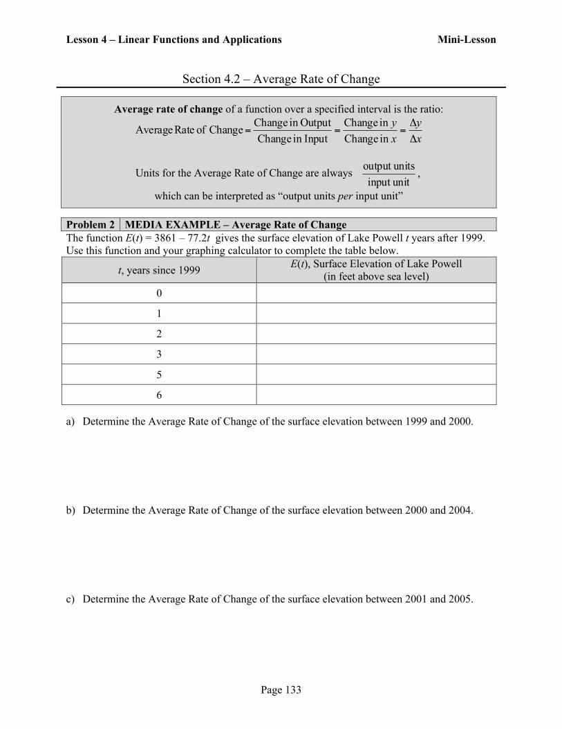
which can be interpreted as “output units per input unit” Problem 2 MEDIA EXAMPLE – Average Rate of Change The function E(t) = 3861 – 77.2t gives the surface elevation of Lake Powell t years after 1999. Use this function and your graphing calculator to complete the table below.
t, years since 1999 E(t), Surface Elevation of Lake Powell (in feet above sea level)
0
1
2
3
5
6 a) Determine the Average Rate of Change of the surface elevation between 1999 and 2000. b) Determine the Average Rate of Change of the surface elevation between 2000 and 2004. c) Determine the Average Rate of Change of the surface elevation between 2001 and 2005.
Lesson 4 – Linear Functions and Applications Mini-Lesson
Page 134
d) What do you notice about the Average Rates of Change for the function E(t)? e) On the grid below, draw a GOOD graph of E(t) with all appropriate labels.
Because the Average Rate of Change is constant for these depreciation data, we say that a LINEAR FUNCTION models these data best.
Does AVERAGE RATE OF CHANGE look familiar? It should! Another word for “average rate of change” is SLOPE. Given any two points (x1, y1) and (x2, y2) on a line, the slope is determined by computing the following ratio:
12
12
Inputin ChangeOutputin Change
xxyym
−
−== =
Therefore, AVERAGE RATE OF CHANGE = SLOPE over a given interval.
Lesson 4 – Linear Functions and Applications Mini-Lesson
Page 135
Average Rate of Change
• Given any two points (x1, y1) and (x2, y2), the average rate of change between the points on the interval x1 to x2 is determined by computing the following ratio:
xy
xy
Δ
Δ===
in Changein Change
Inputin ChangeOutputin Change Change of Rate Average
• If the function is LINEAR, then the average rate of change will be the same between any pair of points.
• If the function is LINEAR, then the average rate of change is the SLOPE of the linear function
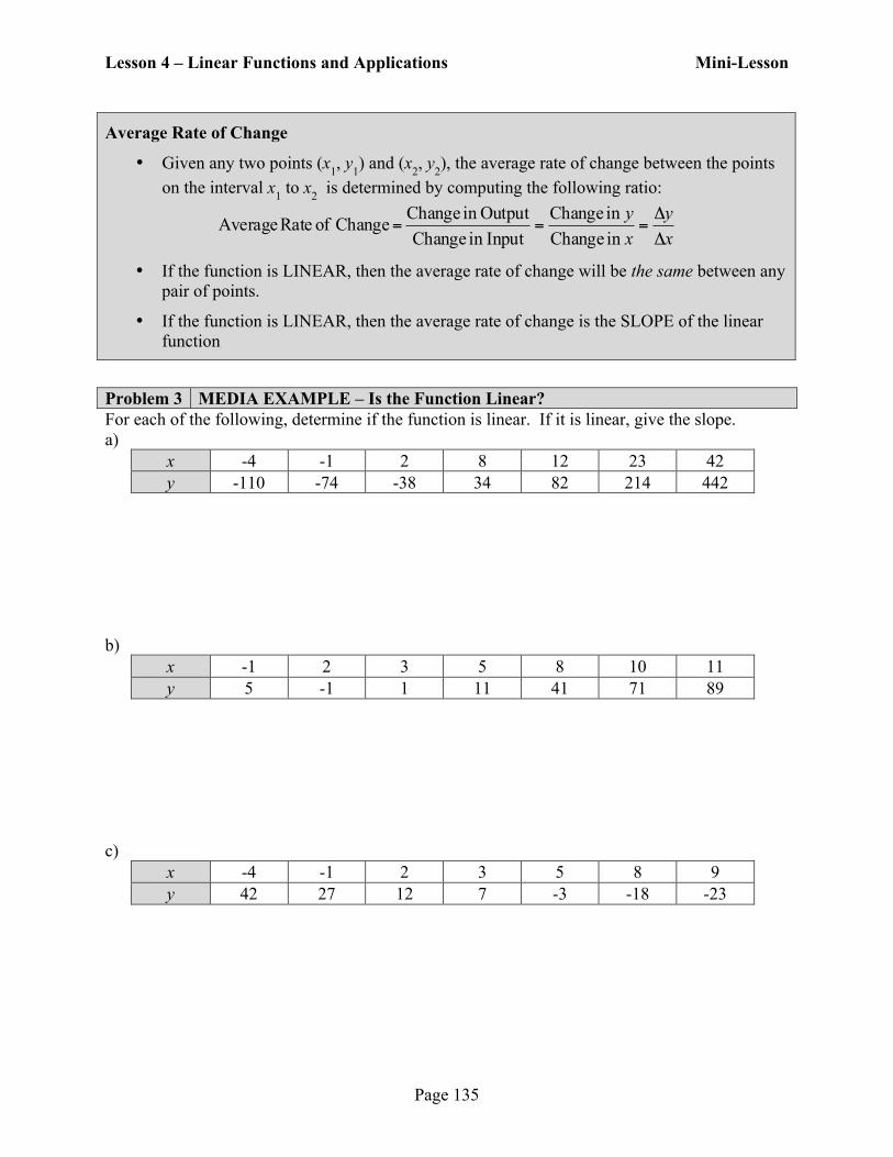
Problem 3 MEDIA EXAMPLE – Is the Function Linear? For each of the following, determine if the function is linear. If it is linear, give the slope. a)
x -4 -1 2 8 12 23 42 y -110 -74 -38 34 82 214 442
b)
x -1 2 3 5 8 10 11 y 5 -1 1 11 41 71 89
c)
x -4 -1 2 3 5 8 9 y 42 27 12 7 -3 -18 -23
Lesson 4 – Linear Functions and Applications Mini-Lesson
Page 136
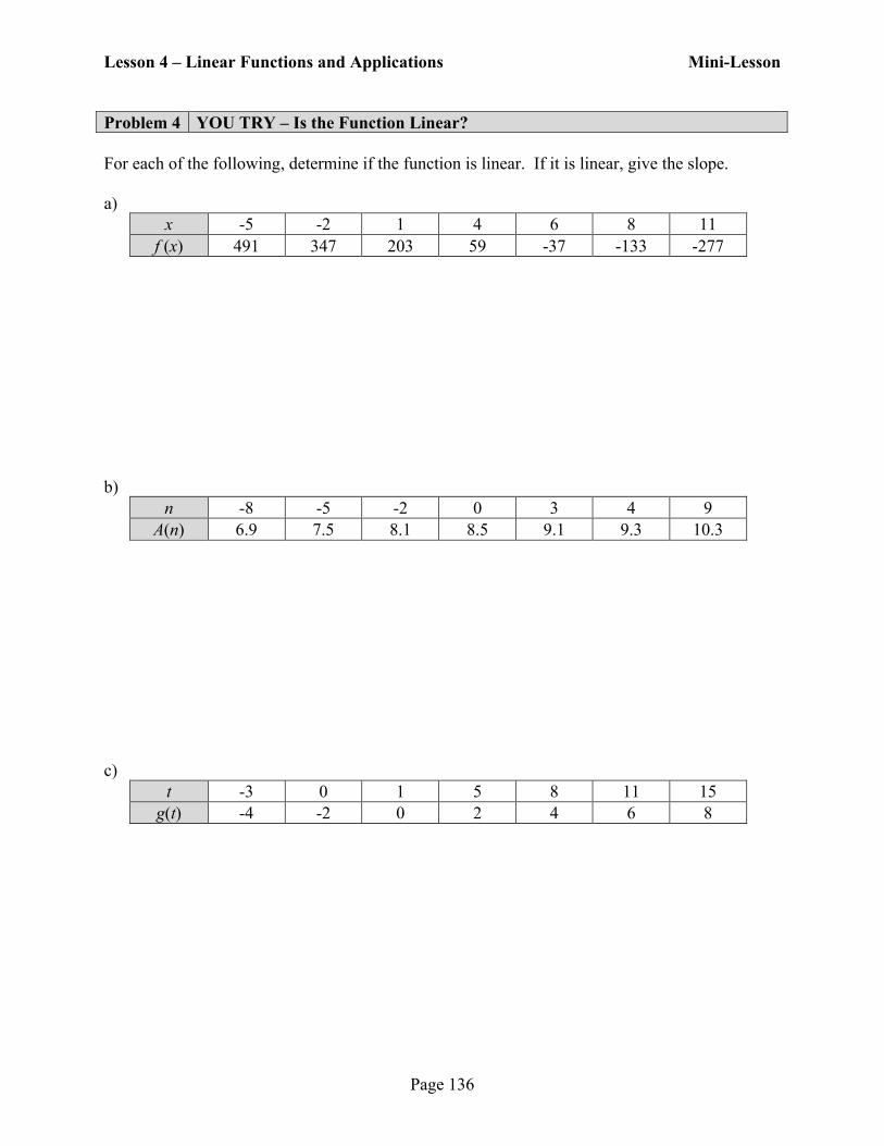
Problem 4 YOU TRY – Is the Function Linear? For each of the following, determine if the function is linear. If it is linear, give the slope. a)
x -5 -2 1 4 6 8 11 f (x) 491 347 203 59 -37 -133 -277
Lesson 4 – Linear Functions and Applications Mini-Lesson
Page 137
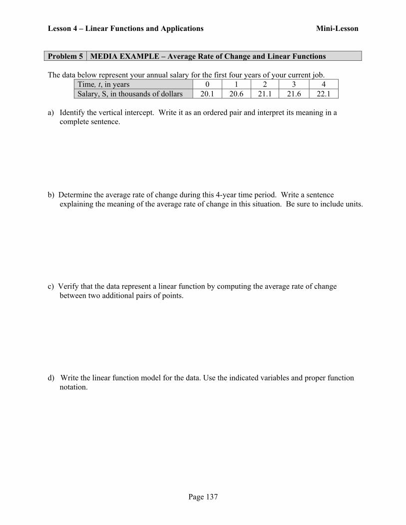
Problem 5 MEDIA EXAMPLE – Average Rate of Change and Linear Functions The data below represent your annual salary for the first four years of your current job.
Time, t, in years 0 1 2 3 4 Salary, S, in thousands of dollars 20.1 20.6 21.1 21.6 22.1
a) Identify the vertical intercept. Write it as an ordered pair and interpret its meaning in a
complete sentence.
b) Determine the average rate of change during this 4-year time period. Write a sentence
explaining the meaning of the average rate of change in this situation. Be sure to include units. c) Verify that the data represent a linear function by computing the average rate of change
between two additional pairs of points. d) Write the linear function model for the data. Use the indicated variables and proper function
notation.
Lesson 4 – Linear Functions and Applications Mini-Lesson
Page 138
Problem 6 YOU TRY – Average Rate of Change
The data below show a person’s body weight during a 5-week diet program.
Time, t, in weeks 0 1 2 3 4 5 Weight, W, in pounds 196 192 193 190 190 186
a) Identify the vertical intercept. Write it as an ordered pair and write a sentence explaining its meaning in this situation. b) Compute the average rate of change for the 5-week period. Be sure to include units. c) Write a sentence explaining the meaning of your answer in part b) in the given situation. d) Do the data points in the table define a perfectly linear function? Why or why not? e) On the grid below, draw a GOOD graph of this data set with all appropriate labels.
Lesson 4 – Linear Functions and Applications Mini-Lesson
Page 139
Section 4.3 – Scatterplots on the Graphing Calculator Consider the data set from the previous problem:
Time, t, in weeks 0 1 2 3 4 5 Weight, W, in pounds 196 192 193 190 190 186
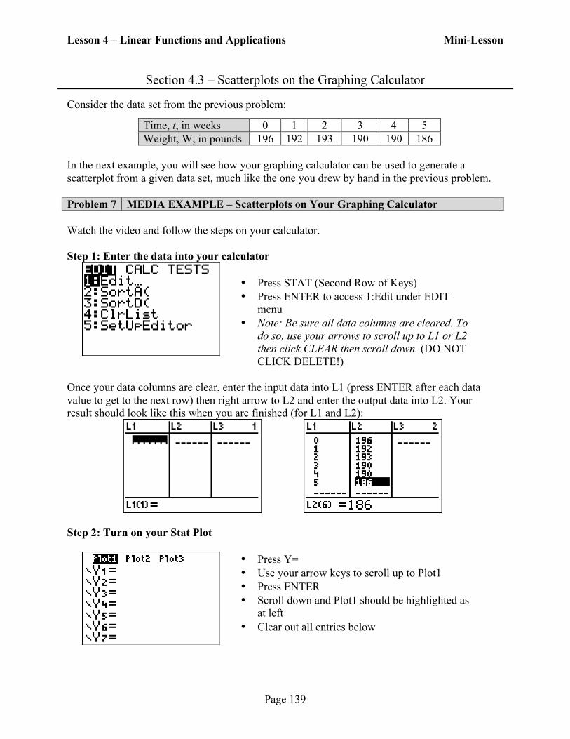
In the next example, you will see how your graphing calculator can be used to generate a scatterplot from a given data set, much like the one you drew by hand in the previous problem. Problem 7 MEDIA EXAMPLE – Scatterplots on Your Graphing Calculator Watch the video and follow the steps on your calculator. Step 1: Enter the data into your calculator
• Press STAT (Second Row of Keys) • Press ENTER to access 1:Edit under EDIT
menu • Note: Be sure all data columns are cleared. To
do so, use your arrows to scroll up to L1 or L2 then click CLEAR then scroll down. (DO NOT CLICK DELETE!)
Once your data columns are clear, enter the input data into L1 (press ENTER after each data value to get to the next row) then right arrow to L2 and enter the output data into L2. Your result should look like this when you are finished (for L1 and L2):
Step 2: Turn on your Stat Plot
• Press Y= • Use your arrow keys to scroll up to Plot1 • Press ENTER • Scroll down and Plot1 should be highlighted as
at left • Clear out all entries below
Lesson 4 – Linear Functions and Applications Mini-Lesson
Page 140
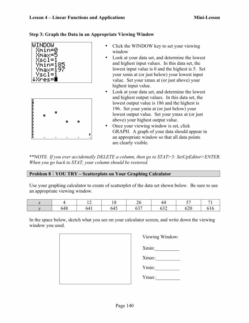
Step 3: Graph the Data in an Appropriate Viewing Window
• Click the WINDOW key to set your viewing
window • Look at your data set, and determine the lowest
and highest input values. In this data set, the lowest input value is 0 and the highest is 5. Set your xmin at (or just below) your lowest input value. Set your xmax at (or just above) your highest input value.
• Look at your data set, and determine the lowest and highest output values. In this data set, the lowest output value is 186 and the highest is 196. Set your ymin at (or just below) your lowest output value. Set your ymax at (or just above) your highest output value.
• Once your viewing window is set, click GRAPH. A graph of your data should appear in an appropriate window so that all data points are clearly visible.
**NOTE If you ever accidentally DELETE a column, then go to STAT>5: SetUpEditor>ENTER. When you go back to STAT, your column should be restored. Problem 8 YOU TRY – Scatterplots on Your Graphing Calculator Use your graphing calculator to create of scatterplot of the data set shown below. Be sure to use an appropriate viewing window.
x 4 12 18 26 44 57 71 y 648 641 645 637 632 620 616
In the space below, sketch what you see on your calculator screen, and write down the viewing window you used.
Viewing Window: Xmin:__________
Xmax:__________
Ymin:__________
Ymax:__________
Lesson 4 – Linear Functions and Applications Mini-Lesson
Page 141
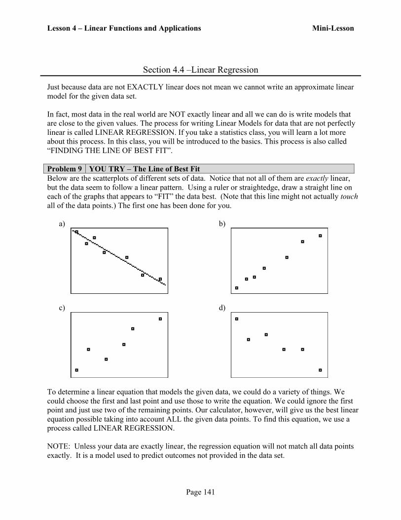
Section 4.4 –Linear Regression Just because data are not EXACTLY linear does not mean we cannot write an approximate linear model for the given data set. In fact, most data in the real world are NOT exactly linear and all we can do is write models that are close to the given values. The process for writing Linear Models for data that are not perfectly linear is called LINEAR REGRESSION. If you take a statistics class, you will learn a lot more about this process. In this class, you will be introduced to the basics. This process is also called “FINDING THE LINE OF BEST FIT”. Problem 9 YOU TRY – The Line of Best Fit Below are the scatterplots of different sets of data. Notice that not all of them are exactly linear, but the data seem to follow a linear pattern. Using a ruler or straightedge, draw a straight line on each of the graphs that appears to “FIT” the data best. (Note that this line might not actually touch all of the data points.) The first one has been done for you.
a)
b)
c)
d)
To determine a linear equation that models the given data, we could do a variety of things. We could choose the first and last point and use those to write the equation. We could ignore the first point and just use two of the remaining points. Our calculator, however, will give us the best linear equation possible taking into account ALL the given data points. To find this equation, we use a process called LINEAR REGRESSION. NOTE: Unless your data are exactly linear, the regression equation will not match all data points exactly. It is a model used to predict outcomes not provided in the data set.
Lesson 4 – Linear Functions and Applications Mini-Lesson
Page 142
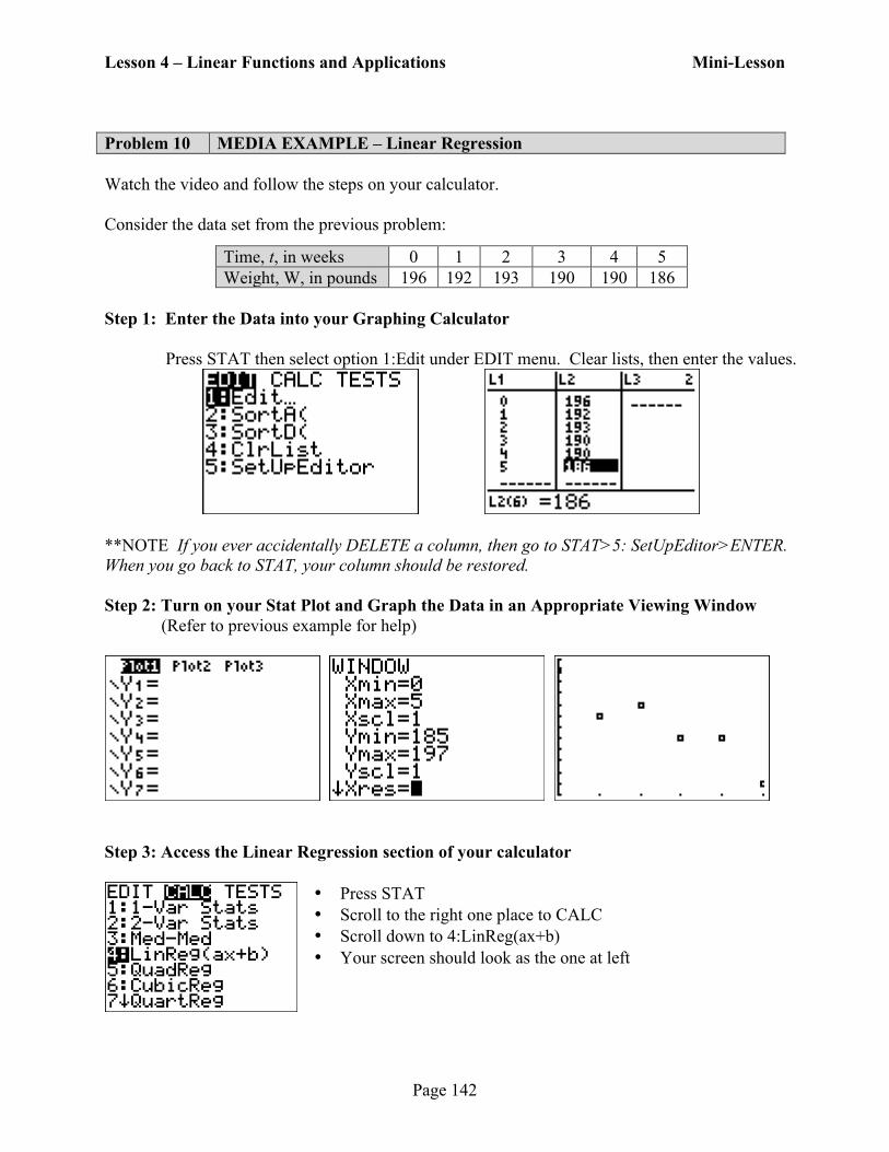
Problem 10 MEDIA EXAMPLE – Linear Regression Watch the video and follow the steps on your calculator. Consider the data set from the previous problem:
Time, t, in weeks 0 1 2 3 4 5 Weight, W, in pounds 196 192 193 190 190 186
Step 1: Enter the Data into your Graphing Calculator Press STAT then select option 1:Edit under EDIT menu. Clear lists, then enter the values.
**NOTE If you ever accidentally DELETE a column, then go to STAT>5: SetUpEditor>ENTER. When you go back to STAT, your column should be restored. Step 2: Turn on your Stat Plot and Graph the Data in an Appropriate Viewing Window (Refer to previous example for help)
Step 3: Access the Linear Regression section of your calculator
• Press STAT • Scroll to the right one place to CALC • Scroll down to 4:LinReg(ax+b) • Your screen should look as the one at left
Lesson 4 – Linear Functions and Applications Mini-Lesson
Page 143
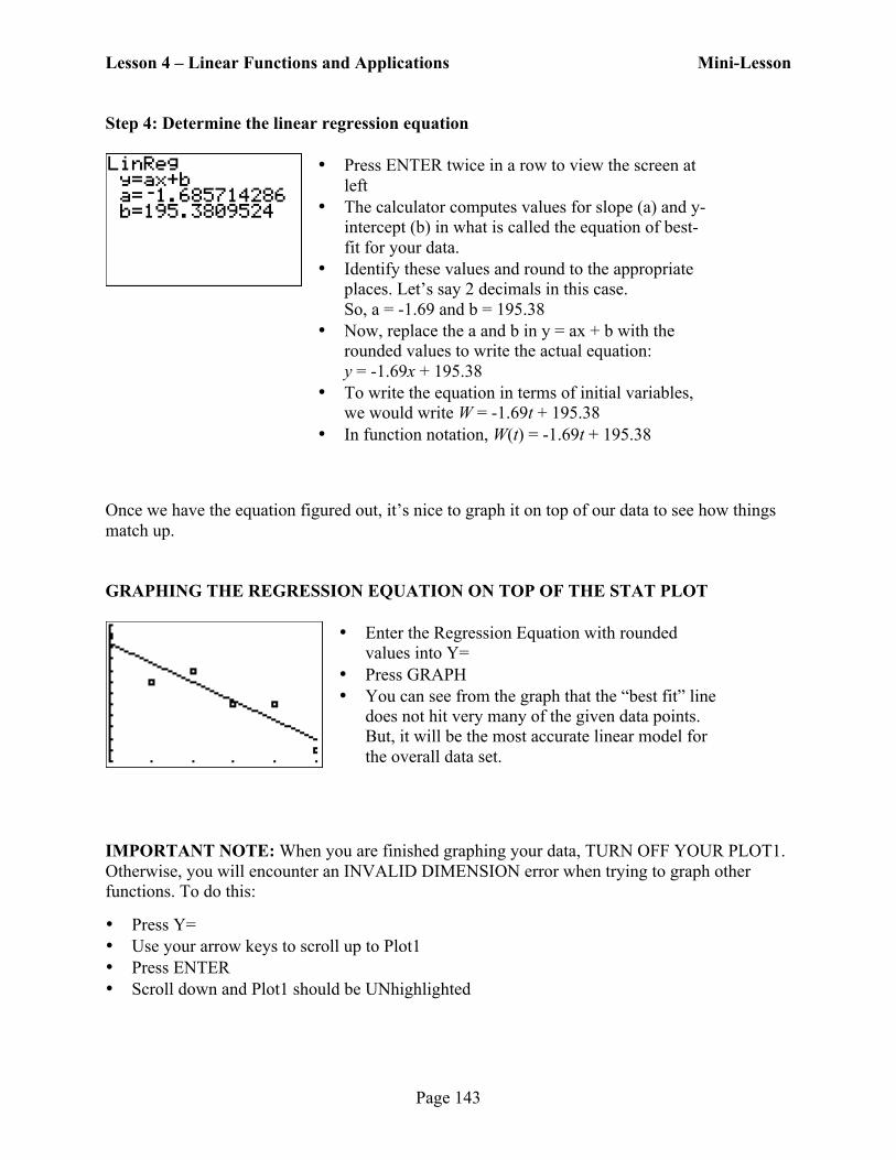
Step 4: Determine the linear regression equation
• Press ENTER twice in a row to view the screen at left
• The calculator computes values for slope (a) and y-intercept (b) in what is called the equation of best-fit for your data.
• Identify these values and round to the appropriate places. Let’s say 2 decimals in this case. So, a = -1.69 and b = 195.38
• Now, replace the a and b in y = ax + b with the rounded values to write the actual equation: y = -1.69x + 195.38
• To write the equation in terms of initial variables, we would write W = -1.69t + 195.38
• In function notation, W(t) = -1.69t + 195.38 Once we have the equation figured out, it’s nice to graph it on top of our data to see how things match up. GRAPHING THE REGRESSION EQUATION ON TOP OF THE STAT PLOT
• Enter the Regression Equation with rounded values into Y=
• Press GRAPH • You can see from the graph that the “best fit” line
does not hit very many of the given data points. But, it will be the most accurate linear model for the overall data set.
IMPORTANT NOTE: When you are finished graphing your data, TURN OFF YOUR PLOT1. Otherwise, you will encounter an INVALID DIMENSION error when trying to graph other functions. To do this:
• Press Y= • Use your arrow keys to scroll up to Plot1 • Press ENTER • Scroll down and Plot1 should be UNhighlighted
Lesson 4 – Linear Functions and Applications Mini-Lesson
Page 144
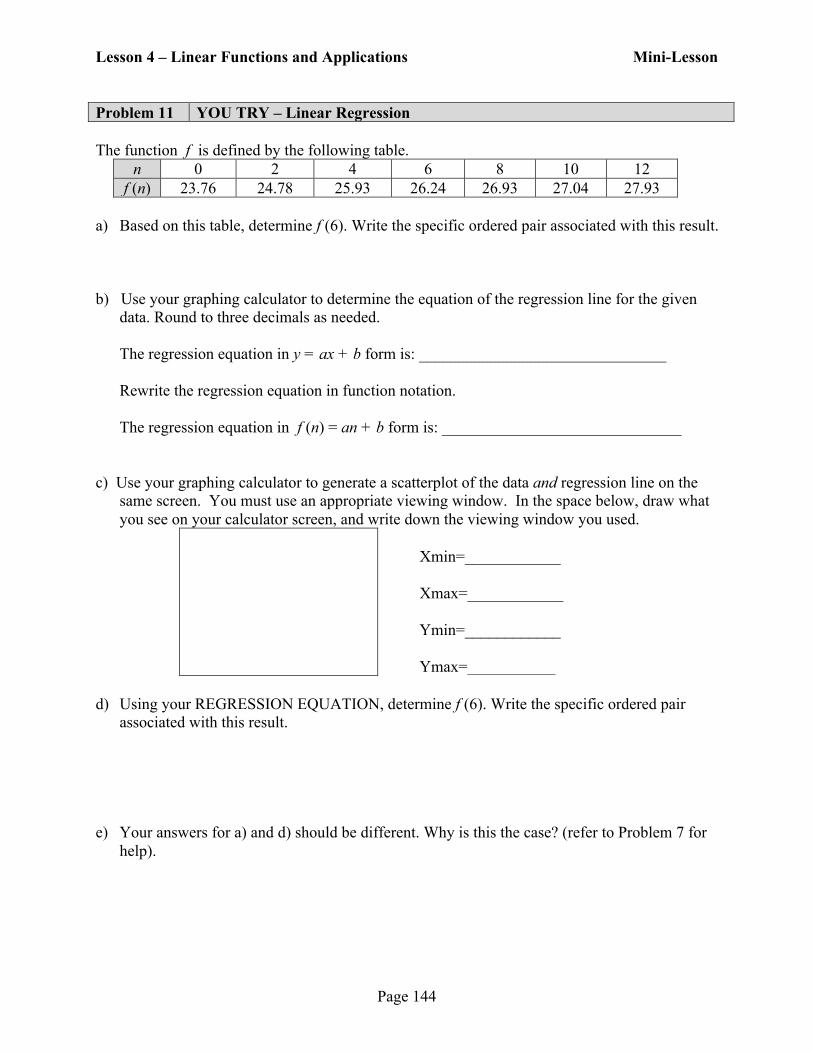
Problem 11 YOU TRY – Linear Regression The function f is defined by the following table.
n 0 2 4 6 8 10 12 f (n) 23.76 24.78 25.93 26.24 26.93 27.04 27.93
a) Based on this table, determine f (6). Write the specific ordered pair associated with this result.
b) Use your graphing calculator to determine the equation of the regression line for the given
data. Round to three decimals as needed.
The regression equation in y = ax + b form is: _______________________________
Rewrite the regression equation in function notation. The regression equation in f (n) = an + b form is: ______________________________
c) Use your graphing calculator to generate a scatterplot of the data and regression line on the
same screen. You must use an appropriate viewing window. In the space below, draw what you see on your calculator screen, and write down the viewing window you used.
d) Using your REGRESSION EQUATION, determine f (6). Write the specific ordered pair
associated with this result. e) Your answers for a) and d) should be different. Why is this the case? (refer to Problem 7 for
help).
Lesson 4 – Linear Functions and Applications Mini-Lesson
Page 145
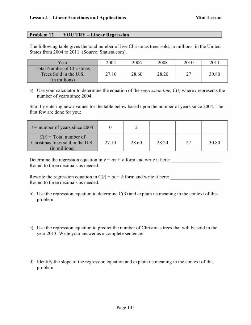
Problem 12 YOU TRY – Linear Regression The following table gives the total number of live Christmas trees sold, in millions, in the United States from 2004 to 2011. (Source: Statista.com).
Year 2004 2006 2008 2010 2011 Total Number of Christmas
Trees Sold in the U.S. (in millions)
27.10 28.60 28.20 27 30.80
a) Use your calculator to determine the equation of the regression line, C(t) where t represents the
number of years since 2004. Start by entering new t values for the table below based upon the number of years since 2004. The first few are done for you:
t = number of years since 2004 0 2
C(t) = Total number of Christmas trees sold in the U.S.
(in millions) 27.10 28.60 28.20 27 30.80
Determine the regression equation in y = ax + b form and write it here: ____________________ Round to three decimals as needed. Rewrite the regression equation in C(t) = at + b form and write it here: ____________________ Round to three decimals as needed. b) Use the regression equation to determine C(3) and explain its meaning in the context of this
problem. c) Use the regression equation to predict the number of Christmas trees that will be sold in the
year 2013. Write your answer as a complete sentence. d) Identify the slope of the regression equation and explain its meaning in the context of this
problem.
Lesson 4 – Linear Functions and Applications Mini-Lesson
Page 146
Section 4.5 – Multiple Ways to Determine the Equation of a Line
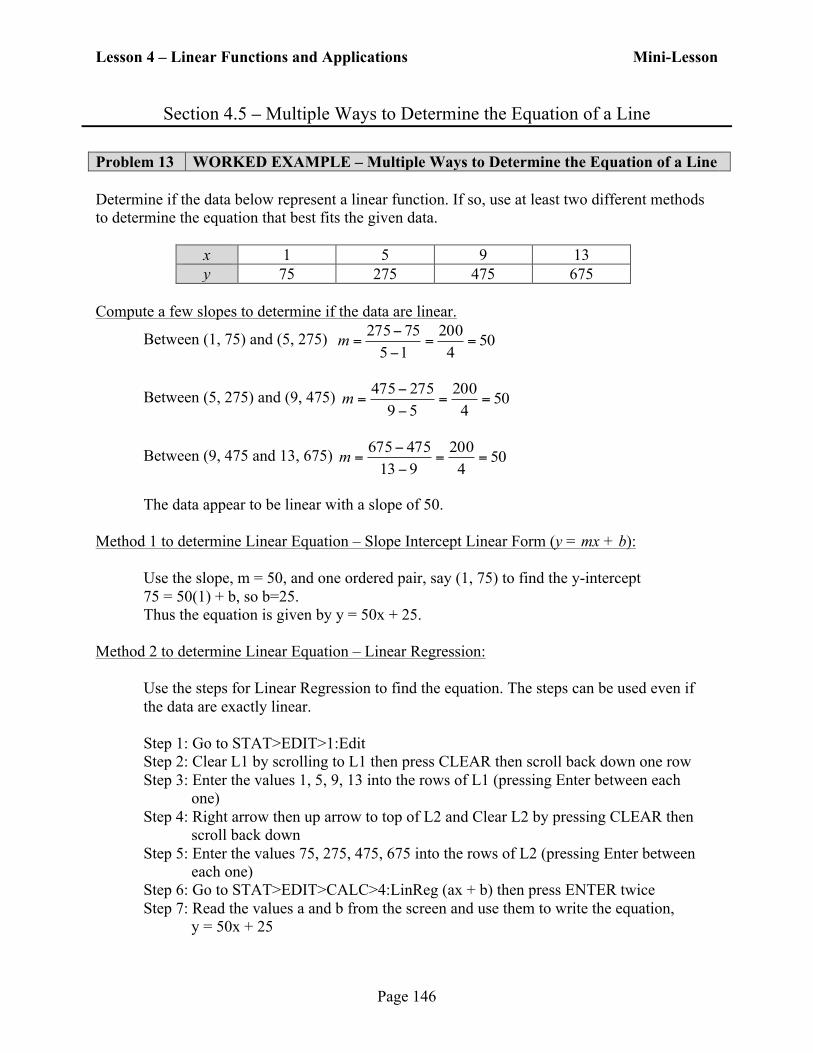
Problem 13 WORKED EXAMPLE – Multiple Ways to Determine the Equation of a Line Determine if the data below represent a linear function. If so, use at least two different methods to determine the equation that best fits the given data.
x 1 5 9 13 y 75 275 475 675
Compute a few slopes to determine if the data are linear.
Between (1, 75) and (5, 275) 504200
1575275
==−−
=m
Between (5, 275) and (9, 475) 504200
59275475
==−−
=m
Between (9, 475 and 13, 675) 504200
913475675
==−−
=m
The data appear to be linear with a slope of 50.
Method 1 to determine Linear Equation – Slope Intercept Linear Form (y = mx + b):
Use the slope, m = 50, and one ordered pair, say (1, 75) to find the y-intercept 75 = 50(1) + b, so b=25. Thus the equation is given by y = 50x + 25.
Method 2 to determine Linear Equation – Linear Regression:
Use the steps for Linear Regression to find the equation. The steps can be used even if the data are exactly linear. Step 1: Go to STAT>EDIT>1:Edit Step 2: Clear L1 by scrolling to L1 then press CLEAR then scroll back down one row Step 3: Enter the values 1, 5, 9, 13 into the rows of L1 (pressing Enter between each
one) Step 4: Right arrow then up arrow to top of L2 and Clear L2 by pressing CLEAR then
scroll back down Step 5: Enter the values 75, 275, 475, 675 into the rows of L2 (pressing Enter between
each one) Step 6: Go to STAT>EDIT>CALC>4:LinReg (ax + b) then press ENTER twice Step 7: Read the values a and b from the screen and use them to write the equation,