136
LICENTIATE THESIS Optimization using discrete event simulation and mixed integer programming: application on haulage systems for deep underground mines Abubakary Salama

LICENTIATE T H E S I S
Department of Civil, Environmental and Natural Resources EngineeringDivision of Mining and Geotechnical Engineering
Optimization using discrete event simulation and mixed integer programming: application on
haulage systems for deep underground mines
Abubakary Salama
ISSN: 1402-1757ISBN 978-91-7439-583-9 (tryckt)ISBN 978-91-7439-584-6 (pdf)
Luleå University of Technology 2013
Abubakary Salam
a Optim
ization using discrete event simulation and m
ixed integer programm
ing
ISSN: 1402-1757 ISBN 978-91-7439-XXX-X Se i listan och fyll i siffror där kryssen är


Optimization using discrete event simulation and mixed integer programming: application on haulage
systems for deep underground mines
Abubakary Salama

Printed by Universitetstryckeriet, Luleå 2013
ISSN: 1402-1757 ISBN 978-91-7439-583-9 (tryckt)ISBN 978-91-7439-584-6 (pdf)
Luleå 2013
www.ltu.se
i
PREFACE
The research work presented herein was performed at the Division of Mining and
Geotechnical Engineering, Luleå University of Technology. This work would not have been
successful without the supports from different people who, in one way or another, participated
in the completion of this work.
Firstly, I would like to give thanks to Professor Håkan Schunnesson for his technical advice, and
support in different aspects of underground mining, which played an important role in the
finalizing of this thesis. I also wish to express my grateful appreciation to Dr. Jenny Greberg for
her valuable materials, suggestions, and ideas towards solving various problems. Her support and
close supervision were highly appreciated.
I would like also to give my warm thanks to the staff members at Division of Mining and
Geotechnical Engineering, and to Dr. Micah Nehring of the University of Queensland for
their support and encouragement, and the recommendations that they provided me with during
the time of this research work.
Special thanks is also due to the University of Dar es Salaam and I2 Mine project within the
EU 7th framework program for the financial support they provided during the time of the
thesis work. I’m also grateful to the management of SimMine for providing me with training
opportunities.
Lastly, to my family, friends, and all those who in one way or another participated in the
preparation and compilation of this paper. Their consideration and patience are gratefully
acknowledged.

ii
iii
ABSTRACT
The application of discrete event simulation for the optimization of the haulage methods of
underground operations at great depth is presented. The discrete event simulation was carried
out to evaluate four haulage methods for the improvement of the overall mine production and
a minimizing of the operating costs. Other techniques can be applied to achieve the same
objective but discrete event simulation is known for its advantage of more accurately
accounting for real world uncertainty and diversity. Discrete event simulation is then
combined with mixed integer programming to improve decision-making in the process of
generating and optimizing the mine plans associated with each hauling option.
The haulage system is one of the most important operations in underground mines as it
involves the transportation of the mined out material from the draw points to the processing
plant. When the depth increases, hauling of ore from deeper levels need to be evaluated in
order to account for the constraints, configuration and current utilization of the ore handling
system for improvement of productivity and operations. The increase in mine depth affects
many factors among which are the increases in haulage distance from mine areas to the mine
surface.
The increase in haul distance results in an increase in the energy cost of the specific hauling
equipment. The haulage process is one of the most energy-intensive activities in a mining
operation and thus one of the main contributors to energy cost. This research uses the
combination of discrete event simulation and mixed integer programing to compare the
operating values of the mine plans generated for an orebody at depth levels of 1,000, 2,000,
and 3,000 meters for diesel and electric trucks, shaft and belt conveyor haulage systems for
the current and future energy prices.
The results shows that, in comparison with analytical methods, discrete event simulation
combined with Mixed Integer Programming (MIP) is faster and generates a more feasible
solution, increases the understanding of the behavior of various systems, and reduces risk
when selecting the operational systems. It is indicated that the energy cost increases as the
mine depth increases and it differs for each haulage method for both current and future energy
prices with higher costs in diesel trucks and lowest costs when using a shaft haulage system.

iv
The energy costs for diesel trucks account for 38.2%, 46.8% and 63.1% of operating costs at
the current energy price, and 64.9%, 72.5% and 83.7% of operating costs at the future energy
prices at the 1,000, 2,000 and 3,000 meter depth levels respectively, while the energy cost for
the shaft haulage system accounts for 10.8%, 13.0% and 15.4% of operating costs at the
current energy price, and for 26.6%, 30.9% and 35.4% of operating costs at the future energy
price at the 1,000, 2,000 and 3,000 meter depth levels respectively. The energy costs is further
analyzed based on haulage costs as a percentage of the total operating cost for all options, and
the results show that diesel truck haulage is substantially more expensive compared to other
haulage options with least energy cost on shaft haulage system with increasing depth. This
study thus provides mining companies operating at great depths, a broad and up-to-date
analysis of the impact on energy costs on the haulage methods as the mine depth increases.
Keywords: Underground haulage system, Production optimization, Equipment selection,
discrete event Simulation, Mixed Integer Programming (MIP), Truck haulage, Shaft system,
Belt conveyor
v
LIST OF APPENDED PAPERS
PAPER A
A.J. Salama and J.Greberg, Optimization of Truck-Loader haulage system in an underground mine: A simulation approach using SimMine. In the proceedings of the 6th InternationalConference and Exhibition on Mass Mining, Sudbury, ON, Canada, 10-14, June, 2012.
PAPER B
Abubakary Salama, Jenny Greberg, and Håkan Schunnesson, The use of Discrete-Event Simulation for underground haulage mining equipment selection. Submitted for publication in the International Journal of Mining and Mineral Engineering
PAPER C
Abubakary Salama, Micah Nehring, Jenny Greberg, Operating Value optimization using Simulation and Mixed Integer Programming. Accepted for publication in the International Journal of Mining, Reclamation and Environment

vi

vii
CONTENTS
1. INTRODUCTION ........................................................................................................................... 1
1.1 Problem statement ......................................................................................................................... 2
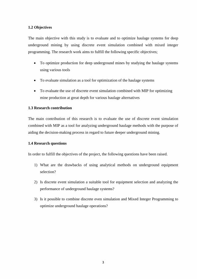
1.2 Objectives ...................................................................................................................................... 3
1.3 Research contribution .................................................................................................................... 3
1.4 Research questions ........................................................................................................................ 3
1.5 Research scope and limitations ..................................................................................................... 4
2. RESEARCH METHODOLOGY .................................................................................................... 5
2.1 Literature review ........................................................................................................................... 5
2.2 Case studies ................................................................................................................................... 6
2.3 Data collection ............................................................................................................................... 6
2.4 Data analysis.................................................................................................................................. 6
3. THEORETICAL FRAME OF REFERENCE ................................................................................. 9
3.1 Haulage systems in deep underground mines.......................................................................... 9
3.1.1 LHD systems ........................................................................................................................ 10
3.1.2 Truck haulage systems ......................................................................................................... 11
3.1.3 Shaft transportation .............................................................................................................. 12
3.1.4 Conveyor belt haulage systems ............................................................................................ 13
3.2 Optimization of haulage systems................................................................................................. 15
3.3 Equipment selection using analytical methods ............................................................................ 17
3.3.1 LHD selection ....................................................................................................................... 17
3.3.2 Truck haulage selection ........................................................................................................ 18
3.3.3 Hoisting shaft selection ........................................................................................................ 19
3.3.4 Belt conveyor selection ........................................................................................................ 20
3.3.5 Drawbacks of using analytical methods ............................................................................... 21
3.4 Haulage system energy consumption .......................................................................................... 22
3.4.1 Dump truck energy consumption ......................................................................................... 22

viii
3.4.2 Hoisting energy .................................................................................................................... 23
3.4.3. Energy to drive the conveyor belt ....................................................................................... 24
3.5 Equipment selection using discrete event simulation .................................................................. 26
3.5.1 Discrete event simulation methods ....................................................................................... 26
3.5.2 Discrete event simulation in mining operations ................................................................... 28
3.5.3 Discrete event simulation tools ............................................................................................ 30
3.5.4 Drawbacks of using discrete event simulation ..................................................................... 31
3.6 Optimization using Mixed Integer Programming (MIP) ............................................................. 31
3.6.1 Mixed Integer Programming (MIP) ...................................................................................... 31
3.6.2 Optimization in underground mining ................................................................................... 32
3.7 Combining discrete event simulation and MIP ........................................................................... 33
4. CASE STUDIES ........................................................................................................................... 35
4.1 Case study I-Haulage system optimization ................................................................................. 35
4.1.1 Model formulation ................................................................................................................ 35
4.1.2 Model verification and validation......................................................................................... 36
4.1.3 Results .................................................................................................................................. 37
4.2 Case study II- optimization of haulage methods based on energy requirements ........................ 40
4.2.1 Model formulation ................................................................................................................ 41
4.2.2 Mixed Integer Programming (MIP) model ........................................................................... 42
4.2.3 Results .................................................................................................................................. 45
5. DISCUSSION ............................................................................................................................... 51
6. CONCLUSIONS .............................................................................................................................. 53
7. FUTURE WORK ............................................................................................................................. 55
REFERENCE ........................................................................................................................................ 57
1
1. INTRODUCTION
As mining companies rapidly exploit near-surface deposits, the mines of the future will be
deeper, more remote, and more hostile, in extreme climatic conditions, with more expensive
energy costs. This will affect the overall economics of mining with increased costs for
material transportation. For many years diesel-powered equipment has become increasingly
utilized in material transportation in mining since its introduction into operations in the 1960s
with significant subsequent efforts to improve productivity and safety. The main advantages
associated with the use of diesel equipment include flexibility in travel routes, flexibility in
the size of the fleet, absence of electrical hazards, high productivity, rapid haulage speed,
generally good reliability and low operating cost (Thomas et al, 1987). The disadvantages of
these vehicles are the use of flammable fuel, higher capital cost, higher heat emission, higher
noise level and emission of toxic gases and particulates into the mine environment which
affects the mine productivity when the mine depth increases (Scott, 1982).
The need to continue using diesel equipment will force mining companies to investigate the
implications of the increased mine operational costs on their mine plan and will emphasize
their need to adapt to different situations. One important aspect of adaptability is to firstly
know what options are available and how a mine plan may be impacted through their
implementation. Several methods can be used to evaluate the haulage options. Due to
presence of random events in the operations, discrete event simulation can be considered as
one among the suitable techniques that can be used for haulage system selection.
Discrete event simulation has in this work been chosen as the operations research
technique for evaluating the mine operations, due to its ability to capture the dynamic and
random nature of the systems. Simulation combined with animation and graphical
representation offers a direct approach to increased understanding of a proposed mining
system. The random and dynamic nature of the mining operations makes it very difficult to
model the operations using analytical models. When simulation is employed, model input can
be based on appropriate probability distributions that characterize the input variables. For the
optimization purpose, discrete event simulation can be combined with Mixed Integer
Programming (MIP) to improve understanding of the behavior of various systems, and reduce
risk when selecting the operational systems. MIP uses a combination of Linear Programming
(LP) and Integer Programming (IP) to define all feasible solutions before using a number of
solution techniques including Simplex Method, Branch and Bound and Cutting Planes to
reach the optimal solution.

2
Simulation and MIP have previously been combined, with simultaneous execution in
order to achieve feasible solutions for operational systems (White and Olson, 1986, Fiorini et
al, 2008,). Fiorini proposed concurrent simulation and optimization models to achieve a
feasible, reliable, and accurate solution to the analysis and generate a short term planning
schedule.
Wilke, 1987 and Chanda, 1990 use the combined tools to model the problem of scheduling
the draw point for mine production optimization. It has been stated that the combined
methodology is more realistic than employing a single technique (Wilke, 1987). For the
purpose of this study, the tools were not simultaneous executed instead discrete event
simulation was used for production estimates for different haulage options, and the results
were used as input in MIP for optimization purposes focusing on minimizing the operating
cost for each haulage scenario.
The research presented in this thesis uses discrete event simulation and Mixed Integer
Programming to analyze and compare the haulage methods for the orebody at depth levels
over 1,000 meters across diesel and electric trucks, shaft and belt conveyor ore haulage
systems with the aim to optimize the overall mine production.
1.1 Problem statement
Currently many underground mines are seeking to operate at greater depth. This has led to
increased haul distances from the working faces to the mine surface, has introduced longer
cycle time for the hauling units and can also generate lower production rates. Hauling
becomes a critical parameter and therefore an effective choice of haulage methods becomes
an important factor in mine production optimization and energy cost minimization for deep
mines.
One of the largest components of the operating costs in underground mining operations is the
energy cost. The use of haulage methods with lower energy consumption will be of great
importance to reduce the operating costs for mining operations at great depth. The lower
energy consumption will also minimize carbon dioxide emissions, which can have the
positive effect of lower additional costs to ventilate the mine.
The research presented in this thesis is carried out using discrete event simulation combined
with MIP to analyze haulage transportation systems for the optimization of the overall mine
throughput and to evaluate the impact of energy requirements associated with each haulage
method.
3
1.2 Objectives
The main objective with this study is to evaluate and to optimize haulage systems for deep
underground mining by using discrete event simulation combined with mixed integer
programming. The research work aims to fulfill the following specific objectives;
To optimize production for deep underground mines by studying the haulage systems
using various tools
To evaluate simulation as a tool for optimization of the haulage systems
To evaluate the use of discrete event simulation combined with MIP for optimizing
mine production at great depth for various haulage alternatives
1.3 Research contribution
The main contribution of this research is to evaluate the use of discrete event simulation
combined with MIP as a tool for analyzing underground haulage methods with the purpose of
aiding the decision-making process in regard to future deeper underground mining.
1.4 Research questions
In order to fulfill the objectives of the project, the following questions have been raised.
1) What are the drawbacks of using analytical methods on underground equipment
selection?
2) Is discrete event simulation a suitable tool for equipment selection and analyzing the
performance of underground haulage systems?
3) Is it possible to combine discrete even simulation and Mixed Integer Programming to
optimize underground haulage operations?

4
The contribution of each paper to each research question is clarified in Table 1.
Table 1. Relationship between appended papers and research questions
APPENDED PAPERS
A B C
RQ1
RQ2 X X
RQ3
1.5 Research scope and limitations
The research presented in this thesis focuses on optimization of different haulage methods
when mine operations are being carried out at great depth based on haulage energy cost and
production different analysis using discrete event simulation combined with MIP. The studied
haulage methods are diesel and electric trucks, shaft, and conveyor belt. The research has
three main limitations:
Rail transportation is one of the energy-efficient modes of transportation in
underground mines but is beyond the scope of this study.
Deposits are analyzed by using metal grades to establish revenues with each resource
block based on an assumed metal price. Uncertainties associated with metal prices and
grade block models will occur over the life of any operation. This leads to a new block
value which result in the generation of a new mine plan. The uncertainties related to
the metal price and grades were not included in this study.
The individual discount rates of various components of the cash flow and the capital
cost of each hauling option were not included in this study.

5
2. RESEARCH METHODOLOGY
Research can be defined as a scientific and systematic search for pertinent information on a
specific topic (Kothari, 2004). The research approach can be conducted by either quantitative
or qualitative methods or a combination of both. A quantitative approach involves the
generation of data in quantitative form such as numbers, measurements and counts (Ghosh,
1982). This approach can be further classified into three categories: inferential, experimental
and simulation. The aim of an inferential approach is to form a database where a sample of a
system is studied to determine its characteristics. An experimental approach is characterized
by the control of research environment and variables are analyzed to observe the effect of
other variables. A simulation approach is used to build models for understanding future
conditions whereby initial conditions and variables are run to represent the behavior of the
process over time. A qualitative approach is concerned with the assessment of attitudes,
opinions, and behaviors using questioning and verbal analysis. In this research, the
quantitative approach is applied, and a literature review, data collection and quantitative
analysis on two case studies were performed.
2.1 Literature review
A literature review was performed on the following topics.
Haulage systems in deep underground mines
Optimization of haulage methods
Energy consumptions of different haulage alternatives
Application of discrete event simulation in underground mines
The use of MIP for optimization of the underground haulage methods
The use of a combination of discrete event simulation and MIP for haulage system
optimization based on energy required for each haulage option.
6
2.2 Case studies
Two case studies were used in this thesis. The first case study examines an underground mine
located in East Africa operated at a depth greater than 1300m. The mine has been in operation
since 2000 and it is expected to be in operation until 2028. The second case study involves an
underground mine located in Australia. It operates at a depth greater than 1500m with an
expected mine life of 13.5 years from 2012.
2.3 Data collection
Discrete event simulation has proved itself to be an effective tool for complex process
analysis (Banks et al, 2000). The drawback of using this method is the effort required and the
costs spent on gathering, collecting and processing the input data from different sources to
ensure valid simulation results. Input data for simulation are needed from many different
production planning and control systems within the mining operations. Data are needed for
building the conceptual model, for model validation, for performing experiments with the
validated model, and for the development of the mathematical and logical relationships used
in the model, allowing the model to adequately represent the problem entity for its intended
purpose. In this research, the following observational data were collected from the East
African mine: cycle time and performance measure of the existing fleet, daily and monthly
production data.
Other data were collected from the Australian mine whereby some of them are
conceptual in nature, the case study is however based on real operational scenarios with stope
tonnages, grades, resource limitations and sequencing interactions reflective of real sublevel
stoping operations, thus making it useful for investigation purposes. The data obtained
include: stope extraction data, the copper price, production planning and scheduling, and
hoisting shaft system data. Some of the data used for belt conveyor design are conceptual in
nature and are taken from the conveyor handbook provided by Fenner Dunlop, 2009. In both
cases, the model formulation was done after data verification and validation using statistical
methods.
2.4 Data analysis
Discrete event simulation analysis was done using SimMine software for Case Study One,
while GPSS/H software was used for simulation and CPLEX software for optimization
purpose in Case Study Two. The SimMine software is based on discrete event simulation

7
principles and uses a full graphical user interface to set up the model and it utilizes statistical
distribution functions to model variations in process times.
General Purpose Simulation System (GPSS) is a versatile computer programming
language originally developed in 1961 to solve various simulation problems which exhibit a
discrete character of events during operation (Schriber, 1989). According to Schriber 1989,
GPSS comprises several modern versions which include GPSS/H, GPSS V/S, GPSS /PC,
GPSS/VX and GPSSR/PC which can be used to model various operations. This research uses
the GPSS/H version in model creation which has been widely used in both open pit and
underground mining operations (Sturgul, 1999), (Harrison and Sturgul, 1989), and (Sturgul
and Singhal, 1988).
CPLEX was used in the construction of Mixed Integer Programming (MIP) models for
the purpose of optimal production scheduling (maximize NPV). CPLEX is optimization
software which can be used to solve a variety of different optimization problems in a variety
of computing environments. The modeling can be done using various mathematical language
programming tools such as AMPL and then solved using CPLEX. It solves linearly or
quadratically constrained optimization problems where the objective to be optimized can be
expressed as a liner function or a convex quadratic function. The variables in the model may
be declared as continuous or further constrained to take only integer values.

8

9
3. THEORETICAL FRAME OF REFERENCE
3.1 Haulage systems in deep underground mines
The haulage system is one of the most important operations in underground mines. It involves
the transportation of the mined out material from the draw points to the loading areas and
continued transportation to the mine surface (Atkinson, 1992). In many underground, hard
rock mines, the haulage system consists of primary and secondary phases. The primary phase
involves the transportation of material from the draw points to the transfer points from where
it is either processed or further transported.
The secondary phase consists of the material transportation from the haulage or loading
areas to the mine surface. In this phase, material can be transported vertically or horizontally.
The vertical hauling methods are shaft, vertical conveyors, skip hoisting, and gravity flow
transportation, while horizontal transportation involves horizontal conveyors, rail, and trucks.
The choice of hauling method depends on various factors among which are included
production requirements, dimensions of the haulage drifts, material fragmentation, capital and
operating cost, production capacity, mining method employed, and other operational features
(Sweigard, 1992). In this research, Load-Haul-Dump (LHDs), diesel and electric trucks, shaft
systems and belt conveyors are discussed. These systems usually contain other supplementary
ore handling components such as feeders, ore passes and crushers. Figure 1 shows a typical
underground mine with several haulage structures such as ramps, shafts and ore passes.
The hauling systems may need fixed or flexible underground infrastructures. Shafts and
conveyor systems can be inflexible because of the limited number of fixed feed points, while
a trucking system is flexible because the trucks can travel to most locations in the
underground mine. In a situation where the underground mine capacity needs to expand to
increase its production capacity, the potential is often related to the configuration and current
utilization of the ore handling system. If the existing hauling method is based on trucks, the
expansion can be achieved incrementally by adding trucks as required until the capacity of the
planned design is reached which may lead to the additional requirement of access and cross
cuts. Increasing throughput in fixed systems such as shafts and conveyors is relatively cheap
up to a point where the system utilization is at the optimal level. Beyond this point, higher
utilization will probably require duplication of the existing system at significant cost. This is
likely to be financially justified only if there is step increase in throughput or geological
information has shown that a system is justified to maintain or create step change in expected
efficiencies and associated operating costs. The hauling methods selected must be flexible

10
enough to accommodate limitations imposed by existing mine facilities, such as compatibility
with production schedule, existing mine development and to cope with different geological
conditions.
Figure 1. A cross section of a typical underground mine (adopted from SME)
3.1.1 LHD systems
Underground loaders are the first components of the ore handling system. Loaders extract ore
from the stope and dump directly into an ore pass or loading bay or load into the trucks that
transport the ore further to the processing plant. Several types of loaders are available which
include rail mounted, rubber-tired loaders, track mounted, and shuttle loaders. Rubber-tired
are commonly used in hard rock mines and are known as LHDs (Load-Haul-Dump). An LHD
may be diesel or electric powered. Diesel units are versatile and can easily move from one
location to another. Electric units carry a cable drum and rely on trailing electric cable, they
have low noise levels and zero emissions, and are highly productive in block caving mines
where ore is transported by a series of draw points to a fixed ore pass location (Atkinson,
1992). In most underground, hard rock mines, manual or automatic LHDs are used to load
and transport the material at this phase due to their effectiveness in transporting material for
short distances (Hartman, 1987).
11
3.1.2 Truck haulage systems
Truck haulage systems are widely used in underground operations for long haul of the
material from the loading bays to the ore pass or shaft station, or directly to the mine surface.
Ore passes are vertical or steeply inclined openings in a rock mass through which broken ore
and waste materials are transported from one mine level to another using gravity flow, while a
shaft is the deep, narrow, vertical hole that gives access to a mine. Trucks used in
underground mining fall into three categories; rigid-body rear dump trucks; articulated rear
dump trucks; and tractor-trailer units with a separate power trailer, usually side dumping. All
have a diesel engine except for trolley-electric trucks, which require a special infrastructure.
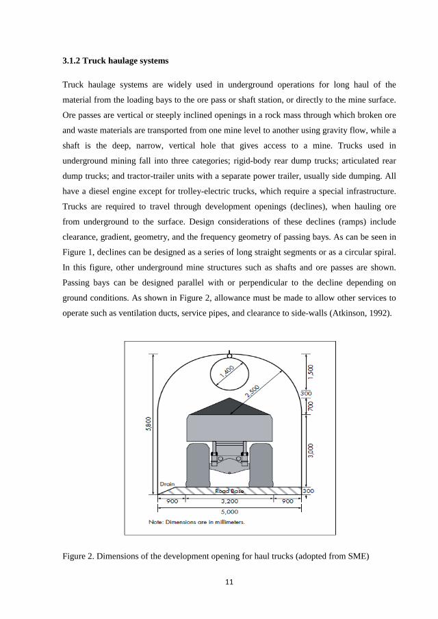
Trucks are required to travel through development openings (declines), when hauling ore
from underground to the surface. Design considerations of these declines (ramps) include
clearance, gradient, geometry, and the frequency geometry of passing bays. As can be seen in
Figure 1, declines can be designed as a series of long straight segments or as a circular spiral.
In this figure, other underground mine structures such as shafts and ore passes are shown.
Passing bays can be designed parallel with or perpendicular to the decline depending on
ground conditions. As shown in Figure 2, allowance must be made to allow other services to
operate such as ventilation ducts, service pipes, and clearance to side-walls (Atkinson, 1992).
Figure 2. Dimensions of the development opening for haul trucks (adopted from SME)

12
The designed dimensions of the declines such as width and curves should include
consideration of vehicle performance. Short curves will slow the vehicle speed, which results
in longer cycle time and hence decreases the productivity. As shown in Figure 3, the width
and grade of the decline haul road should enable vehicles to safely negotiate around curves at
a given speed taking into account sight distance and minimum vehicle turning radius.
Figure 3. Decline dimensions for curve radius (Sandvik)
3.1.3 Shaft transportation
A shaft is one of the most important openings of an underground mine. As can be seen in
Figure 1, shafts are used to access mineral resources which are too deep to be mined
economically using open cut methods. Shafts are also used to provide various services such as
ventilation, power, water supply, etc., to an underground mine. To design a mine shaft,
several variables have to be considered in order to arrive at an economic decision. Such
variables include; length of the shaft, ore and waste tonnage to be handled, ventilation
requirements, capital costs, operating costs, mine machinery handling, and materials handling
(Brucker, 1975).
According to Edward, 1988, the shaft consists of five main components; hoist, wind,
conveyances, ropes, and headframe. Edwards has also identified an additional 277
13
subcomponents. The number of subcomponents and their interrelationship with the main
components indicates the complexity of a shaft-hoisting system. The selected hoisting
equipment is intended for the life-time of the mine and therefore it is important that the proper
choice is made (Beerkircher, 1989). Shaft hoisting systems are equipped with conveyances to
transport material and workers from the underground to the surface. Conveyances are the
skips for ore or waste transportation and cages for transporting workers and other materials
that are suspended by the hoisting ropes.
The hoisting system consists of drum and friction hoists. The drum hoist is usually
located some distance from the shaft and requires a headframe and sheaves to center the
hoisting ropes in the shaft compartment. In this hoisting type, the ropes are stored on a drum.
The Koepe or friction hoist consists of a wheel with a groove lined with friction material to
resist slippage. The hoist ropes are not attached or stored on the wheel instead they are wound
around the drum and over the head sheaves to the conveyances. In the friction hoist,
conveyance positions are fixed relative to each other with tail rope used to counterbalance the
rope loads throughout the hoisting cycle. This lowers the starting torque and requires a
smaller motor to hoist the same load that reduces both capital and operational cost (Harmon,
1973). According to Schulz, 1973, Tudhope, 1973 and Brucker, 1975, a friction hoist with
multiple ropes can carry a higher payload and have a higher output in tons per hour than drum
hoists. Friction hoists have lower pick demand than drum hoists with the same output and
they can operate at lower light power supply. Drum hoists are suitable for higher payloads
when operated at shallow depths. When the depth increases, the drum hoist capacity can be
extended by adding ropes per conveyance, which increases the installation costs.
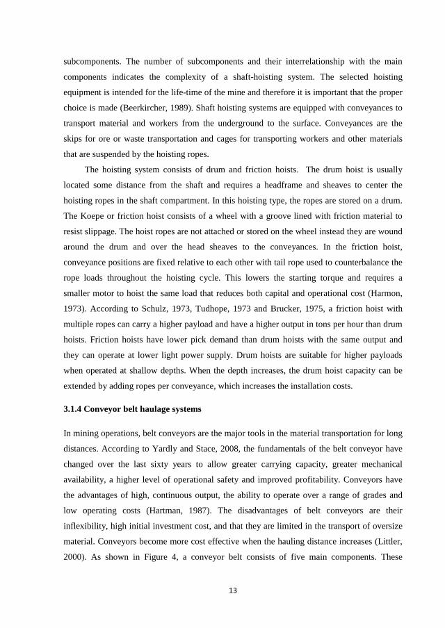
3.1.4 Conveyor belt haulage systems
In mining operations, belt conveyors are the major tools in the material transportation for long
distances. According to Yardly and Stace, 2008, the fundamentals of the belt conveyor have
changed over the last sixty years to allow greater carrying capacity, greater mechanical
availability, a higher level of operational safety and improved profitability. Conveyors have
the advantages of high, continuous output, the ability to operate over a range of grades and
low operating costs (Hartman, 1987). The disadvantages of belt conveyors are their
inflexibility, high initial investment cost, and that they are limited in the transport of oversize
material. Conveyors become more cost effective when the hauling distance increases (Littler,
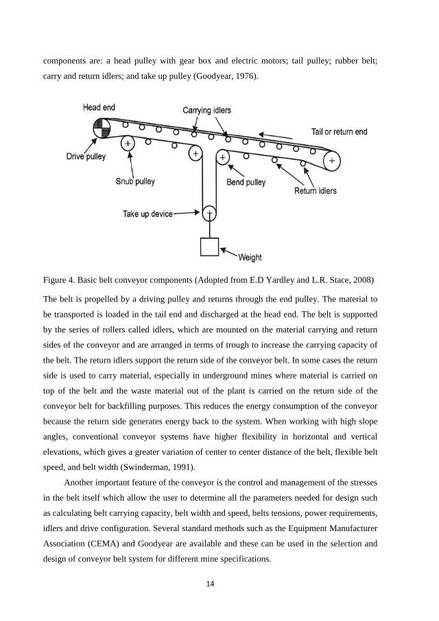
2000). As shown in Figure 4, a conveyor belt consists of five main components. These
14
components are: a head pulley with gear box and electric motors; tail pulley; rubber belt;
carry and return idlers; and take up pulley (Goodyear, 1976).
Figure 4. Basic belt conveyor components (Adopted from E.D Yardley and L.R. Stace, 2008)
The belt is propelled by a driving pulley and returns through the end pulley. The material to
be transported is loaded in the tail end and discharged at the head end. The belt is supported
by the series of rollers called idlers, which are mounted on the material carrying and return
sides of the conveyor and are arranged in terms of trough to increase the carrying capacity of
the belt. The return idlers support the return side of the conveyor belt. In some cases the return
side is used to carry material, especially in underground mines where material is carried on
top of the belt and the waste material out of the plant is carried on the return side of the
conveyor belt for backfilling purposes. This reduces the energy consumption of the conveyor
because the return side generates energy back to the system. When working with high slope
angles, conventional conveyor systems have higher flexibility in horizontal and vertical
elevations, which gives a greater variation of center to center distance of the belt, flexible belt
speed, and belt width (Swinderman, 1991).
Another important feature of the conveyor is the control and management of the stresses
in the belt itself which allow the user to determine all the parameters needed for design such
as calculating belt carrying capacity, belt width and speed, belts tensions, power requirements,
idlers and drive configuration. Several standard methods such as the Equipment Manufacturer
Association (CEMA) and Goodyear are available and these can be used in the selection and
design of conveyor belt system for different mine specifications.

15
One of the problems of belt conveyor systems is maintenance of the operational
components. Maintenance involves a number of routine works, inspection of the various
components and initiating timely repair or servicing of these components in case any failure is
observed. It is therefore important that a number of protective devices are incorporated to save
the belt from getting damaged by operational activities. Also the conveying of sticky material
should be avoided. This is associated with problems of cleaning and discharge causing poor
productivity and increasing delays (Swinderman, 1991).
3.2 Optimization of haulage systems
Mine optimization is one of the important steps in the viability of a mining project.
Approaches for selection of hauling equipment on the basis of minimizing the haulage cost is
one of the main parameters in the optimization process. This thesis focuses on the
optimization of diesel and electric trucks, shafts, and belt conveyor haulage systems in deep
underground mines to determine which of the different kinds of material handling equipment
available will result in the desired production objectives and at the same time lead to the
lowest cost. Shaft systems and belt conveyors incur a large initial fixed cost investment and
rely on the subsequent low operating cost of material movement to the surface. Truck haulage
requires progressive capital expenditure depending on the material flow and has an earlier
recovery of ore in the life of the mine with a higher cost per unit of material moved to the
surface. There are many techniques which are available for equipment selection to both the
construction and mining industries. In mining industry, the equipment selection aimed to meet
materials handling needs at minimum cost in a given mining conditions. The selection process
depends on the mine methods, mine infrastructures, and production capacity. The mining
method selected implies a subset of suitable loads and haul equipment to be used. Figure 5
describes the distribution of equipment selection literature and also lists some techniques that
can be applied in the selection process (Oberndorfer, 1992). Operations research such as
integer programming deals with the application of mathematical sciences to arrive at optimal
or near optimal solutions to complex decision-making problems. Genetic algorithms involve
the selection or search algorithms that are based on the principals of natural selection. They
generate solutions to optimization problems using techniques inspired by natural evolution
such as mutation, selection, and past experience. Petri nets are graphical and mathematical
modeling tool applicable to many systems for the purpose of describing various processes. It
offers a graphical notation for stepwise processes that include choice, iteration, and
concurrent execution (Murata, 1989).

16
Analytical methods use mathematical principals to fully predict the implications of a theory.
They can be used to solve an equation without any degree of estimation. Analytical methods
have been widely used for many years in both open pit and underground operations.
Analytical methods evaluate load and haul combinations and include production constraints
such as road conditions and rock characteristics (Atkinson, 1992) and (Ercelebi and Kirmanli,
2000).
Figure 5. The distribution of various techniques for the equipment selection

17
3.3 Equipment selection using analytical methods
3.3.1 LHD selection
Loading units in combination with haul trucks are used to haul material from the mine areas
to the dumping locations. When selecting this equipment, the size of loaders and trucks is one
of the most important factors to be considered for production optimization. As shown in
Figure 6, the size of the selected loader must fit within the planned development and stope
openings and its maximum bucket reach must not exceed the height of the opening. The
loader should also be able to reach a truck height and fill it efficiently. Its required bucket
capacity can be estimated based on the loader cycle time, bucket volume, broken density of
the rock to be carried, and a fill factor, which depends on rock fragmentation. The theoretical
cycle time for the loader can be calculated by summing up the time to load and unload a
bucket, the time to travel to and from the dumping point, and maneuvering time (Sweigard,
1992). The rock volume is converted into loose volume by the percentage of swell factor. The
fill factor is a factor of the material sizing condition and how easy or difficult it is to fill the
bucket and this can be determined by field measurements (Atkinson, 1992). The maximum
size of bucket is linearly correlated to the size of the machine.
Figure 6. LHD dimensions (Sandvik)

18
3.3.2 Truck haulage selection
Based on the selected loading equipment, the type and number of hauling vehicles is chosen
to fit the loading units and to minimize delays in the operations. The selection of size and type
of the trucks depend on various factors including road geometry, production rate, haulage
distance, mining method, ore reserve tonnage, haul road dimensions, safety, capital and
operating costs, road intersections, required truck speed, corners and bends, road quality, etc.
The size selection also depends on the number of passes used by the loader to load a truck. A
truck with a higher capacity and a loader with low capacity will increase the number of loader
passes required to fill the truck which leads to an extended cycle time for the hauler and hence
lower production.
The optimal combination of loading and hauling units in an operation can be obtained based
on what is known as the “match factor” (Lizotte and Bonates, 1987). This factor was first
formulated by the Caterpillar Company to quantify the apparent balance that exists between
the numbers of loading units and haul units. The factor is defined as shown in equation 1.
ctyl
ctyh
HNLN
MF**
(1)
Where MF stands for match factor, hN represents number of haul units, lN is the number of
loading units, ctyL and ctyH are the load and haul cycle times respectively. When MF is below
1, it indicates that the system is under-trucked, while if it is above 1, it shows that the system
is over-trucked. If it is exactly 1, it means that there is a theoretical match between haulers
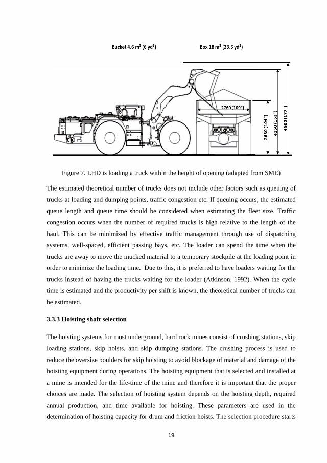
and loaders and that a loader is efficient for the loading of a truck, as seen in Figure 7. The
Match Factor calculations only provide an estimate of the optimal balance between loader and
trucks. The total number of vehicles however, also depends on the estimated truck cycle time,
productivity estimate, available time in a shift, etc. The cycle time depends on the truck speed
for different road grades, grade resistance and rolling resistance. If the road grades and
resistances are higher, the speeds of the haul units will be reduced, leading to an increased
cycle time.
19
Figure 7. LHD is loading a truck within the height of opening (adapted from SME)
The estimated theoretical number of trucks does not include other factors such as queuing of
trucks at loading and dumping points, traffic congestion etc. If queuing occurs, the estimated
queue length and queue time should be considered when estimating the fleet size. Traffic
congestion occurs when the number of required trucks is high relative to the length of the
haul. This can be minimized by effective traffic management through use of dispatching
systems, well-spaced, efficient passing bays, etc. The loader can spend the time when the
trucks are away to move the mucked material to a temporary stockpile at the loading point in
order to minimize the loading time. Due to this, it is preferred to have loaders waiting for the
trucks instead of having the trucks waiting for the loader (Atkinson, 1992). When the cycle
time is estimated and the productivity per shift is known, the theoretical number of trucks can
be estimated.
3.3.3 Hoisting shaft selection
The hoisting systems for most underground, hard rock mines consist of crushing stations, skip
loading stations, skip hoists, and skip dumping stations. The crushing process is used to
reduce the oversize boulders for skip hoisting to avoid blockage of material and damage of the
hoisting equipment during operations. The hoisting equipment that is selected and installed at
a mine is intended for the life-time of the mine and therefore it is important that the proper
choices are made. The selection of hoisting system depends on the hoisting depth, required
annual production, and time available for hoisting. These parameters are used in the
determination of hoisting capacity for drum and friction hoists. The selection procedure starts

20
with the cycle time calculation, which is later used to estimate skip payload for the hoisting
system. The cycle time is the total time the hoist system takes to move a conveyance from the
bottom of its wind to the top and depends on the initial creep, acceleration, and full speed,
deceleration, dumping, loading and resting. When cycle time and the annual production rate
are known, the skip payload which is expressed in terms of the average tonnage per hours
hoisted can be determined using equation 2.
Payload = Production rate (tonnes/hours) (2)Cycle time (second) x 3600(second/hour)
Based on the skip size and production rate, the type and size of rope can be established. For
both hoisting systems, the rope selection is based on the safety factors, compatibility, rope life
and rope cost. The life of the rope is usually affected by the number of trips it will make, hoist
and sheave dimensions, type of loading, and maintenance. When a friction hoist system is
used, the number of ropes must be defined, while for drum hoist a single rope of high strength
can be selected. The selection should also be based on strength, resistance to failure, abrasion
resistance, and resistance to distortion to ensure safety in moving the material, personnel and
other services (Edward, 1988).
3.3.4 Belt conveyor selection
The starting point of conveyor design has to be a knowledge of what has to be moved, how far
it has to be moved, the gradient over which has to be moved, and what constraints there might
be to the design of the conveyor. When designing a conveyor system, the choice of width and
speed will be influenced by the nature of the material to be conveyed, available tunnel space,
and the overall economics of the system. Other factors that need to be considered in the
design include the ability of the belt to conform properly to the trough formed by the idlers
and the effect on the belt of forming the trough. The trough angle which the conveyor can
adopt relative to the horizontal is limited by the tendency of the material to slide down the belt
or to move internally relative to itself (Ketelaar and Davidson, 1995).
The selection of conveyor belts considers various parameters such as belt width,
surcharge angle, belt speed, inclination angle, troughing angle, driving and takes up pulleys,
motors, and idler configuration. These parameters influence the performance of the conveyor
and are considered when estimating of the belt carrying capacity and power requirement. The
21
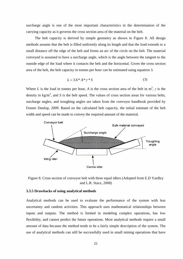
surcharge angle is one of the most important characteristics in the determination of the
carrying capacity as it governs the cross section area of the material on the belt.
The belt capacity is derived by simple geometry as shown in Figure 8. All design
methods assume that the belt is filled uniformly along its length and that the load extends to a
small distance off the edge of the belt and forms an arc of the circle on the belt. The material
conveyed is assumed to have a surcharge angle, which is the angle between the tangent to the
outside edge of the load where it contacts the belt and the horizontal. Given the cross section
area of the belt, the belt capacity in tonnes per hour can be estimated using equation 3.
(3)
Where L is the load in tonnes per hour, A is the cross section area of the belt in m2, is the
density in kg/m3, and S is the belt speed. The values of cross section areas for various belts,
surcharge angles, and troughing angles are taken from the conveyor handbook provided by
Fenner Dunlop, 2009. Based on the calculated belt capacity, the initial estimate of the belt
width and speed can be made to convey the required amount of the material.
Figure 8. Cross section of conveyor belt with three equal idlers (Adopted from E.D Yardley and L.R. Stace, 2008)
3.3.5 Drawbacks of using analytical methods
Analytical methods can be used to evaluate the performance of the system with less
uncertainty and random activities. This approach uses mathematical relationships between
inputs and outputs. The method is limited in modeling complex operations, has low
flexibility, and cannot predict the future operations. Most analytical methods require a small
amount of data because the method tends to be a fairly simple description of the system. The
use of analytical methods can still be successfully used in small mining operations that have
SAL ***6.3

22
less uncertainty, but most large mining operations need methods that will involve
randomness.
3.4 Haulage system energy consumption
Haulage of material from underground to the mine surface leads to higher energy
consumption than other mining operations. This makes energy costs one of the largest
components of the operating costs in underground mining operations. This means that haulage
methods that exploit lower energy consumption will be of great significance in the reduction
of the operating costs for mining operations at great depth (Kecojevic and Komljenovic,
2010).
In this research, discrete event simulation and MIP were used to compare the energy
consumption for hauling the ore from depth levels of 1,000, 2,000, and 3,000 meters to the
mine surface for diesel trucks, electric trucks, shaft and belt conveyor haulage systems both at
the current and estimated future energy prices. The aim is to evaluate the energy requirements
associated with each haulage method at each mine depth.
3.4.1 Dump truck energy consumption
The energy consumption by dump trucks depends on the hauling distance from the loading
point to the dumping point, payload, vehicle speed, mine topography, engine capacity, and the
load factor. With a short hauling distance, trucks can produce a higher output at low operating
costs compared to when they work at great depth where the haul distance from the draw
points to the mine surface increases which leads to an increase in the operating costs
(Kecojevic and Komljenovic, 2010). In this research, diesel and electric trucks are analyzed
to compare energy consumption for variable mine depths. During the study, both truck types
were simulated based on similar working conditions. Diesel trucks can effectively travel on
steeper grades, have a large market presence, and require a low level of technical
specialization. Electric trucks typically travel at higher speed on steeper grades up to 20%,
have potentially low maintenance cost, offer slightly better fuel economy, have a smoother
operator ride and offer better retarding capacity to stop the truck. However they do have
higher capital cost and require electricity lines. During loading and dumping, electric trucks
leave the trolley line and use a motor driven by diesel.
When a truck moves, the engine generates power against friction, tire rolling resistance
and gradient resistance. The energy consumed can be estimated using equation 4 (Kecojevic
and Komljenovic, 2010).

23
= (4)
Where LMPH is the liters used per machine hour, K stands for the kilograms of fuel used per
brake horsepower per hour, GHP represents the gross engine horsepower at governed engine
revolution per minute, KPL is the weight of fuel in Kg/liter, and LF is the load factor in
percentage. The load factor is defined as the portion of full power required by the truck.
According to (Caterpillar, 2009), the engine load factors are termed as:
Low: 20%-30%, low load factor, excellent haul road condition, no overloading
Medium: 30%-40%, moderate road factor, good haul road condition, minimal
overloading,
High: 40%-50%, high load factor, poor haul road condition, overloading.
The energy consumption of the electric truck depends on the engine size, operator efficiency,
and condition of the equipment and was estimated based on load factor, condition of the
equipment and gross engine horsepower.
3.4.2 Hoisting energy
In the case study presented in this research, a friction or Koepe hoisting system with two
swing-out body skips in balance and four flattened-strand ropes was selected. Friction hoist
has an ability to handle heavy loads with comparatively smaller mechanical equipment
configurations resulting in smaller power drives compared to a drum hoist. The main factor in
the determination of the required hoisting power of the shaft system is the duty cycle of the
hoist. The duty cycle is the relationship between hoist powers and hoisting cycle time. The
plot of duty cycle for a friction sheave hoist is shown in Figure 9. This figure shows the
horsepower needed (HP) to drive the hoisting system depending on the skip speed,
acceleration and deceleration rates, creep speeds and distances and is indicated as HP1 to HP6
(Harmon, 1973). The hoisting cycle time consists of three major activities: skip loading, skip
travel, and skip unloading. The skip load is estimated based on calculated cycles and used in
the determination of the rope strength to ensure safe working conditions. The power
estimation for the hoisting system at different mine depth was determined after integrating the
area under the curves and is shown in equation 5 (Harmon, 1973).

24
25 *108.19)(***7457.0
xTFSATVW
E o (5)
Where E is the power consumption for duty cycle in KWh/trip, Wo is the skip live load, V
stands for the hoisting velocity, AT is the acceleration time, TFS is the constant-velocity time,
and is the hoisting efficiency as a decimal.
Figure 9. Power estimation per cycle time for friction hoist system (adopted from SME, 2003)
3.4.3. Energy to drive the conveyor belt
Belt conveyors are widely used in the mining industry to move the mined material from the
working faces or storages to the different parts of the mine or to the mine surface. Conveyors
are normally driven by motors. The motors that are used for this purpose are AC induction
motors due to their low operating costs. When material is moved by the belts, electrical
energy is converted into various forms of energy such as movement energy, potential energy,
noise energy, and heat energy. The energy conversion model gives the relationship between
energy to drive the conveyor and the conveyor parameters (Hiltermann et al, 2011). There are
different models available that are used to estimate the required power to drive the conveyor
system such as CEMA (Conveyor Equipment Manufacturers Association), Goodyear, FDA
(Fenner Dunlop Australia), etc. In this research, the Goodyear model was used. The technique
was chosen due to its wide applicability for bulk solids material handling (Hiltermann et al,
2011). The model states that the required power to drive the conveyor consists of three types
of power. The power needed to run the empty conveyor, the power required for moving the
25
material horizontally over a certain distance, and the power needed to lift the material to a
certain elevation. The assumptions that are made are the introduction of an artificial friction
coefficient to allow the evaluation of the main resistance and the introduction of a length
coefficient to allow the secondary resistances to be calculated. To run the empty belt, the
power required to move different parts of the conveyor is described as shown in equation 6
(Hager & Hintz, 1993) where Pec is the power required to run the empty belt in kilowatts
(KW), g is the acceleration due to gravity in m/s2, C is the friction factor, Q is the mass of
moving parts of the conveyor in kg/m, L stands for the distance of incline and decline belt, L0
is the horizontal center to center distance, S is the belt speed, and t is the hours where the belt
is in operation.
tSLLQCgPec *1000
*)(*** 0 (6)
The power required to move the material horizontally over a certain distance was calculated
based on equation 7 (Hager & Hintz, 1993) where Ph is the power to move the material
horizontally and T stands for the transfer rate in tons per hour.
tTLLCgPh *3600
*)(** 0 (7)
When the belt is moving material at an inclined section or lowering the material at the decline,
the power consumption can be obtained as shown in equation 8 (Hager & Hintz, 1993) where
Pl is the power to raise or lower the load, and H is the changing in elevation.
tHTgPl *3600
** (8)
The total power consumed by the conveyor belt can be obtained by summation of equations 6,
7, and 8 and can be given as shown in equation 9 (Hager & Hintz, 1993).
lhect PPPP (9)
As it can be seen in the power consumption equations, the power required to run the empty
conveyor is dependent on the speed of the belt. This illustrates that the conveyor belt is
energy-efficient when it is running under full load conditions, a factor that should be taken
into consideration when the electricity cost efficiency of the belt conveyor is investigated.
26
3.5 Equipment selection using discrete event simulation
3.5.1 Discrete event simulation methods
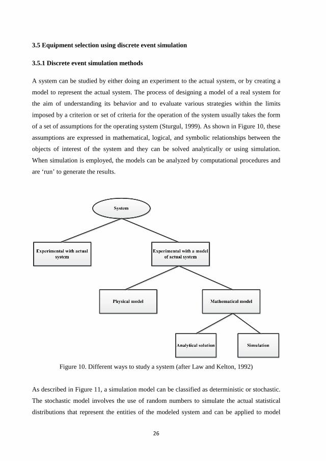
A system can be studied by either doing an experiment to the actual system, or by creating a
model to represent the actual system. The process of designing a model of a real system for
the aim of understanding its behavior and to evaluate various strategies within the limits
imposed by a criterion or set of criteria for the operation of the system usually takes the form
of a set of assumptions for the operating system (Sturgul, 1999). As shown in Figure 10, these
assumptions are expressed in mathematical, logical, and symbolic relationships between the
objects of interest of the system and they can be solved analytically or using simulation.
When simulation is employed, the models can be analyzed by computational procedures and
are ‘run’ to generate the results.
Figure 10. Different ways to study a system (after Law and Kelton, 1992)
As described in Figure 11, a simulation model can be classified as deterministic or stochastic.
The stochastic model involves the use of random numbers to simulate the actual statistical
distributions that represent the entities of the modeled system and can be applied to model

27
discrete or continuous operations (Law and Kelton, 1991). Continuous simulation is used
when the system variables can be represented by differential equations that calculate the rates
of change of the variable with respect to time. Typically continuous simulation models are
solved by deterministic methods such as differential equations. Deterministic means that once
a set of initial conditions has been specified, the output can be determined by solving the
equations.
Figure 11: System model taxonomy (after Law and Kelton, 1992)
Discrete event simulation has been used in the mining industry for many years (Sturgul
1995b). It deals with the modelling of a system over time by representing the changes as
separate events. Separate event means that time advances until the next event occurs.
Examples of the discrete event systems that can be simulated are business processes,
transportation logistics, mining operations, emergency response system, etc. During
modeling, system events advance by variable or fixed intervals. In variable event simulations,
the time of occurrence for the next event is determined and the simulation clock is advanced
to this value, while with fixed interval advances, time is increased at fixed intervals. This
method tends to be slower in the computation as the computer processes through various
routines regardless of whether the system has changed state or not (Law and Kelton, 1991).
Discrete event simulation also applies different types of rules and procedures that increase the
understanding of the interaction between variables and their importance in the system
performance and provide suggestions on modification availabilities in the system (Banks,
2000).

28
3.5.2 Discrete event simulation in mining operations
Discrete event simulation is not new to the mining industry. It has been applied since the
1960s to simulate various mining problems mainly in connection with transport systems
(Zhao and Suboleski, 1987). Operations such as fleet requirements, the flow of hauling
machines and mine planning, (with the aim of optimizing, improving, analyzing and planning
of the existing and future systems), can be modeled using simulations. Sturgul provides a
comprehensive review of mine system simulation literature covering the period 1961-1995
(Sturgul, 1996). In the past, mine simulation models have been created using programming
languages such as FORTRAN. Nowadays the models are created with more specific mine
simulation tools such as general purpose programming languages which have the ability to
import the three dimensional vector-based graphics for superior animations.
Discrete event simulation has been established to handle complex mining systems
which are discrete, change dynamically over a certain time and can be operated within a
variable economic environment. It is used worldwide to solve these types of problems
(Panagiotou, 1999). The use of this technique in mining operations was first reported by Rist
(1961). Since then several studies has shown a wide applicability of simulation studies on
various operations in both underground and open pit mines in the world (Raj et al, 2009).
The United States mining industry was among the first to recognize the importance of
simulation for use in mine planning and mine design (Sturgul, 1999). During the first
symposium on the use of computers in mining, a paper on computer simulation of a mine
operation was published by Rist (1961), where a model was built to determine the optimum
number of trains for a haulage level. Since then, the use of simulation has progressed to
several mining aspects such as queuing theory, scheduling, decision-making, location models,
etc. One of the examples is truck-shovel simulation in a copper mine to simulate if dispatchers
could be used to route the trucks to different shovels so as to minimize queuing time and
improve the preparation (Sturgul, 1999). In Europe, the first mine simulations appeared in
1950s in the northern part of Sweden to model the train transportation at the Kiirunavaara
underground iron mine. The model was done by hand (Elbrond, 1964). Thereafter the
development of the use of discrete simulation became more widespread in several countries.
Mutagwaba and Durucan (1993) report an example from the United Kingdom where a
simulation model for a mine transportation system was developed. Other examples include
development of a simulation model to study the train transportation in underground coal
mines in Germany (Wilke, 1970), and development of a computer program that assists in
29
analyzing shovel-truck operations in the mines. Recently, the use of discrete event simulation
has become even more popular in mining operations in Europe with studies in Sweden,
Germany, Turkey, etc (Panagiotou, 1999).
In South African mines, simulation has emerged as a useful means to explore the
impact of new capital investments and any proposed mining method. It has also been used in
existing mines for planning, optimization, and selection of equipment (Turner, 1999). An
example of a case study using simulation is the Ingwe Douglas Piller project where a
simulation was conducted to determine the truck-shovel combinations suitable for the
proposed mining operation. In Xu and Dong (1974), the application of discrete event
simulation to develop a computer model of shovel and truck transportation system for an open
pit mine in China was presented. The technique is well spread to both coal and hard rock
mines for the analysis of the haulage system. In Russia, computer simulation has been used
for underground mining since the 1980s for developing the best correlations of the capacities
of the haul units (Konyukh et al, 1999). In Australia simulation has been used in various
mining applications. An early project using a computer simulation to develop the ore handling
operations of the Mt. Newman Mining Company in Port Hedland, Western Australia, was
published in 1989 (Basu and Baafi, 1999). After that several projects for both surface and
underground mining in coal and hard rock areas have been carried out such as the use of
simulation modeling to optimize the underground ore handling at the Cadia East Mine,
(Greberg and Sundqvist, 2011).
In South America, there are several large copper, iron and bauxite mines that are
operated in various countries. Example of these are the Chuquicamata and Escondida
operations in Chile, the CVRD Carajas Mine in Brazil which operates the largest iron ore
open pit in the world, and the Cerrejon Coal Mine which operates the largest truck fleet in the
world (Knights and Bonates, 1999). The starting point for the use of discrete event mine
simulation in South America was difficult to ascertain due to the fact that there was no
established science or engineering citation service.
Knight and Bonates, 1999, reported that several simulation models were developed in
the 1980s. These models have been used to simulate the entire mining operation with varying
degrees of success. One of the earliest papers relating to simulation modeling in South
America is by Nogueira, 1984, which describes the application of a simulation model to
improve truck-shovel operation at the CVRD Mine in Brazil. The model was designed to
assess the best truck/shovel combinations in order to determine the capacity of the mine
operation. Another model was developed at Codelco Chile’s Teniente Mine using GPSS/H

30
and PROOF animation (Sturgul, 1999). The model uses discrete simulation to simulate a
system with continuous state variables, the t-test was performed to test the simulated results
and hypothetically the decision to accept or reject the hypothesis was made.
Generally, discrete event simulation modeling is a useful tool for mine planning and
design, machine selection and designing the haulage system with the aim to optimizing the
mine operation and production throughputs. Early studies focused mainly on limited parts of
the mining process, such as for instant, equipment selection for the development stage, while
more recent studies have aimed to cover more parts of the system and even to simulate a
complete mine.
3.5.3 Discrete event simulation tools
The use of discrete event simulation tools increases the understanding of the system
performance and the interaction of the many variables involved. Discrete event simulation
tools can be divided into three categories (Banks et al, 2010). First, general purpose
programming languages, such as Java, C, and C++, which offer a high degree of flexibility at
a low cost, but require high programming skills (Sturgul and Jacobson, 1994). Programs
written in general purpose simulation languages have been applied for the development of
discrete event simulation software packages for both underground and open pit operations
(Sturgul 1999). The second category involves simulation programming languages, such as
GPSS/H, SIMAN, AUTOMOD, etc. These types of software are object-oriented, discrete
system simulation languages with high flexibility and they also require good knowledge of
programming and are relatively expensive.
The third category is simulation language environment. This is a special computer
language containing features that can be applied to different applications. Models are created
by writing a program using the model elements with little or no coding. Models are created
using graphics and built-in modeling elements. The most popular simulation language
environments found in the mining industry include SLAM, AUTOMOD, SIMUL 8,
SimMine, etc. Due to the availability of a large number of simulation software options,
careful selection should be made depending on the type of problem to be simulated.
According to Yuriy and Vayenas, 2008, there are many issues to consider when selecting the
software for the simulation studies. Some of these include: ease of use; availability of
adequate debugging and error diagnostics; ability to import data from other software such as
computer aided design and spreadsheet; availability of animation environment for easy
visualization of the operations; quality of the output report; and graphs for interpretation.
31
3.5.4 Drawbacks of using discrete event simulation
Discrete event simulation has an ability to model complex systems in great detail and to
provide more accurate results. A verified and validated simulation model could provide
results that are very close to those seen in the actual operating system. The high accuracy
comes at the expense of high modeling and computational effort. Developing a detailed, more
accurate simulation model for a large and complex system requires the collection of a large
amount of data; the fitting of the data to statistical distributions; and considerable care in the
choice of simulation software. The probabilistic nature of many events such as ramp grade
variation, haul truck speeds, and machine failures can be represented by sampling from the
probabilistic distribution behavior of the data representing a pattern showing the occurrence
of the event. Failure to fit data to the correct distributions may result in an inaccurate
estimation of the system performance. Thus, to represent a typical behavior of the system, and
obtain performance measure estimates with high confidence levels, it is necessary to run the
simulation model many times so that many events can occur a large number of times.
3.6 Optimization using Mixed Integer Programming (MIP)
3.6.1 Mixed Integer Programming (MIP)
Mixed Integer Programming (MIP) is recognized within mathematical science groups as a
tool to model and find the optimal solution to large, complex, and highly constrained
problems such as the problem being addressed in this case. The application of MIP models
varies extensively from transportation scheduling and distribution of goods to production
planning in manufacturing (Winston and Goldberg, 2004). In the past, the use of MIP in the
mining industry has been somewhat confined to open pit applications (Lerchs and Grossman,
1965).
However, recently it has become more extensively used in the underground
environment. Trout, 1995, scheduled production within the Mount Isa Mine, Australia, with
emphasis on stope development and backfilling process, however he was unable to solve MIP
to optimality due to the large number of binary variables. Almgren 1994 used MIP as an aid
in scheduling development and production at the Kiirunavaara Mine and he also run into the
difficulties in solving the large-scale MIP due to the time-dynamic nature of his initial
problem formulation. In the past, the use of MIP has been hindered because models of real
world problems must often incorporate a large number of decision variables, many of which
32
must assume integer values. Because of the large number of integer variables, solution times
may be unacceptably long for practical planning purposes. Currently model formulation using
MIP is created by processing the production data and formulating the model carefully which
reduces the number of binary and integer variables in a multi-period production model and
thus greatly reduces solution times and leads to the optimal solution (Newman et al, 2007).
MIP uses a combination of Linear Programming (LP) and Integer Programming (IP) to
define all feasible solutions before using a number of solution techniques including the
Simplex Method, Branch and Bound and Cutting Planes to obtain the optimal solution. The
shortfall in current computer processing power however, has constrained the more extensive
use of this technology (McIsaac, 2005). It is therefore vital that efficient modelling takes
place to reduce the number of variables and in turn reduce solution time.
3.6.2 Optimization in underground mining
Optimization of mine plans for the purpose of maximizing net present value using Operations
Research (OR) techniques can be categorized into three main areas (Alford, 1995), including:
production schedule optimization, stoping limit optimization and infrastructure placement
optimization. These three core areas themselves incorporate numerous other sub-factors (cut-
off grade policy, mill throughput/recovery relationship, environmental factors), which are
currently largely predetermined or dealt with in a sequential manner such that the solution for
one forms the starting point to solve the next (Nehring et al, 2010). While these processes are
largely treated as separate individual components in the overall system, future research must
focus on combining these areas into one common model in order to achieve truly optimal
integrated results.
Optimization of production schedules is considered the most advanced of the three main
areas in mine planning. Numerous works by various authors (Ataee-Pour (2005), Brazil and
Thomas (2004), Carlyle and Eaves (2001), and Topal (2008)) have shown that with clever and
efficient modelling the production scheduling problem can be solved for increasingly larger
datasets. The increased ability to solve far more complex problems also allows further
integration of other key sub-factors including key environmental cost factors affecting mine
sites such as the consumption of water and energy and the release of carbon. The development
of further efficiencies in modelling these complex problems will, in time, also advance the
ability to integrate the three main areas mentioned above in the development of an integrated
and comprehensive mine planning optimization tool.

33
One recent development of particular interest has been an MIP model that integrates
short and long-term production plans by combining the short term objective of minimizing
deviation from targeted, mill feed grade with the long-term objective of maximizing net
present value (NPV) into a single mathematical optimization model. The development of
short and long-term mine production schedules in isolation from each other had previously
meant that only a local optimum could be achieved when each scheduling phase was carried
out. The global optimal solution, however, can be achieved when integrating scheduling
phases and accounting for the interaction between short and long-term activities
simultaneously.
Another recent development of interest is an integrated production scheduling and stope
boundary optimization model for underground sublevel stoping operations. This model, based
on MIP, takes the very first steps in generating the global optimal integrated production
schedule / stoping boundary definition problem for the purpose of maximizing net present
value. As acknowledged by the author of this research, this model still needs many
improvements and ultimately needs to also incorporate infrastructure placement in order
integrate and capture all three key areas simultaneously.
3.7 Combining discrete event simulation and MIP
The discrete event simulation was combined with MIP to increase the efficiency of the
analyzed systems, to improve the understanding of the behavior of various systems and
reduce risk when selecting the operational systems. For the purpose of this thesis, the discrete
event simulation method is used to estimate the energy in Kilowatt-hour (KWh) for each
haulage option. MIP is carried out by analyzing the simulation results and extrapolating a set
of actual operating costs for a typical sublevel stoping operation and then optimizing the
energy costs. The currency used for the purpose of this thesis is Australian dollar per ton
mined for each haulage scenario.

34

35
4. CASE STUDIES
4.1 Case study I-Haulage system optimization
In this case study, the haulage system of an East African mine was optimized using SimMine
software. Currently, the mine operates at 1300m depth with an annual production of 2.62Mt
pyrite and chalcopyrite ore. The mine uses four different mining methods: sublevel open
stoping, drift and fill, narrow vein, and Alimak. The focus in this study is on the sublevel open
stoping mining method. In this part of the mine, three LHDs are assigned to operate, on three
different stopes, and three trucks haul the ore from each stope to the shaft. Currently, this
vehicle fleet only produces 52% of the planned production. It is assumed that the reasons for
the low production are the limited size of drifts, the ramp design, and traffic interference in
the ramps, etc. All these factors increase the cycle time of the trucks, reducing overall
equipment effectiveness and mine output. The haulage system is simulated in order to
optimize the number of trucks for the studied mine production system, to increase the mine
output and to evaluate the possibilities to reach the assigned production targets. Furthermore,
in order to optimize production, a productivity comparison is also made for two different
types of trucks. Truck type one is a TH430, which has a theoretical capacity of 25-30 tonnes.
Truck type two is a TH660 with a payload of 50-55 tonnes.
4.1.1 Model formulation
The model was developed by importing the mine layout into SimMine software. The layout
includes a 5.5m width ramp, loading bays, 3.5m height production drifts, and 100m length of
cross cuts. There are 7 production drifts each ranging from 250m to 400m in length, with an
average vertical distance of 17m (floor to roof) and connected by a ramp. Each drift contains
several stopes, with a 20-25m strike length and an average thickness of 3.5m. Ore from all
production drifts are transported to a single dumping point at a shaft location. In this part of
the mine, the general mine sequence allows 3 stopes to be mined simultaneously. Due to the
limited size of the drifts, only 1 LHD can be used in each production drift. During the
simulation, the number of TH430 or TH660 trucks was changed from 3 to 9. Thus, each LHD
serves 1 to 3 trucks.
The LHD tramming distance depends on the length of the production drift. The
tramming distance is defined as the distance from the active face to the loading bay. The cycle
time will be longer for vehicles working at the far end of the drift than for vehicles in the
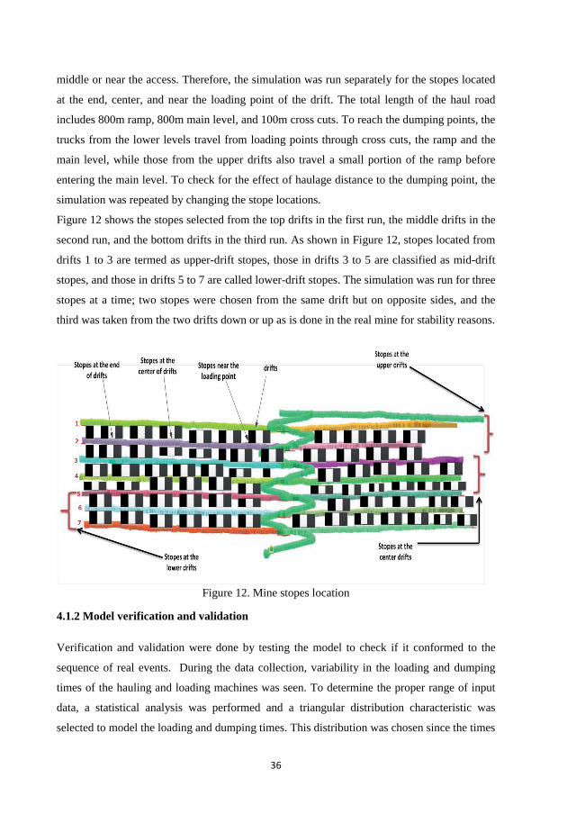
36
middle or near the access. Therefore, the simulation was run separately for the stopes located
at the end, center, and near the loading point of the drift. The total length of the haul road
includes 800m ramp, 800m main level, and 100m cross cuts. To reach the dumping points, the
trucks from the lower levels travel from loading points through cross cuts, the ramp and the
main level, while those from the upper drifts also travel a small portion of the ramp before
entering the main level. To check for the effect of haulage distance to the dumping point, the
simulation was repeated by changing the stope locations.
Figure 12 shows the stopes selected from the top drifts in the first run, the middle drifts in the
second run, and the bottom drifts in the third run. As shown in Figure 12, stopes located from
drifts 1 to 3 are termed as upper-drift stopes, those in drifts 3 to 5 are classified as mid-drift
stopes, and those in drifts 5 to 7 are called lower-drift stopes. The simulation was run for three
stopes at a time; two stopes were chosen from the same drift but on opposite sides, and the
third was taken from the two drifts down or up as is done in the real mine for stability reasons.
Figure 12. Mine stopes location
4.1.2 Model verification and validation
Verification and validation were done by testing the model to check if it conformed to the
sequence of real events. During the data collection, variability in the loading and dumping
times of the hauling and loading machines was seen. To determine the proper range of input
data, a statistical analysis was performed and a triangular distribution characteristic was
selected to model the loading and dumping times. This distribution was chosen since the times

37
are fairly uniform around the mean, but not symmetrical. The load and haul unit properties
show that loading time per pass differs for the two truck types because of both the loading
capacity and the height of the truck boxes. The TH430 has a box height of 2.3m and a
capacity of 30 tonnes, while the TH660 has a box height of 3.4m and a capacity of 60 tonnes.
The loading unit needs more passes and lifting time to fill truck TH660 than truck TH430.
4.1.3 Results
The simulation was first conducted for the stopes located at the upper drifts in order to
compare with the real mine case. Currently the mine operates with 3 LHDs and three TH430
trucks (one assigned to each LHD). In relation to schedule production, based on the design
and the overall mine plan, the set up with three LHDs and three TH430 trucks only produces
52% of the planned production. As can be seen in Figure 13, the results show that when
considering TH430 for three trucks served with three LHDs, the amount of ore produced is
52.5% which indicates that the result is close to the real operation in the mine. With 4 and 5
trucks in operation each LHD will serve one predetermined truck, while the extra trucks will
be directed from dispatch to move to the LHD that has no queue.
When the TH 430 is in operation, the production is sharply increased when the number of
trucks is increased from 3 to 6. Beyond this point, the amount of ore produced does not rise at
the same rate as the drop in truck utilization. The increased number of trucks leads to a
reduction in truck utilization for both truck types with the lowest utilization values noticed
when operations are in the stopes located at the end of the drift leading to increased LHD
utilizations. The higher LHD performance is observed when they work for the stopes at the
end of drifts. It can be seen in Figure 13 that the traffic is minimal when three trucks are in
operation, but the traffic increases when the number of trucks starts to increase. The term
traffic refers to the percentage of time lost when trucks meet in the haul ways (the main drift
and the ramp). The highest percentage of traffic is when the LHDs are working near the
loading point, due to the short waiting times for the trucks at the loading point and thus the
longer time spent for transportation on the main level where other trucks are present. It is
observed that among all the simulated scenarios, a combination of 2 trucks and a single LHD
for the upper drifts and 3 trucks and 1 LHD for the lower or mid drifts improves the average
production to 75% of planned production.

38
Figure 13. Simulation results for the TH430 at upper drifts
The simulation was then run on the same locations for a productivity comparison between the
TH430 and TH660 truck types. As shown in Figure 14, for stopes on the upper drifts, the
amount of ore produced at the end, center, and near the loading bay seems to be slightly
higher for the TH660 than that of TH430 even though the pay load for the TH660 is twice as
high as for the TH430. In all cases, the amount of ore produced increases as the number of
trucks increases. It also observed that production is greater when these trucks are working on
the stopes located in the upper drifts than those in the mid and lower drifts because trucks in
the latter two cases have a longer time to complete the cycle than the trucks in the former.
Trucks working on the upper drifts have a longer waiting time at the loading point than those
on the mid and lower drifts due to their short time to complete the cycle. The truck waiting
time increases when operations are going on at the far end of the drift. In this case, the LHDs
spend more time loading and hauling material from the face to the loading point because of
the longer tramming distance. Normally, automatic LHDs are used to muck the material
immediately after the stope has been blasted and dumped at the stockpile located at the
loading point of each production drift. This reduces the loss of time when normal loading
equipment is in operation. During this operation, the manual LHDs and haul trucks are not
working due to the unsafe condition of the stope. After the stope has been stabilized, the
loading equipment will start mucking the stope and loading the trucks. When there is no truck
waiting at the loading point, the LHDs will also dump the material at the stockpile.
2 4 6 8 100
10
20
30
40
50
60
70
80
90
No. of Trucks
Pe
rce
nta
ge
(%
)
End of the drift
2 4 6 8 100
10
20
30
40
50
60
70
80
90Center of the drift
No. of Trucks
Pe
rce
nta
ge
(%
)
2 4 6 8 100
10
20
30
40
50
60
70
80
90Near the loading point
No. of Trucks
Pe
rce
nta
ge
(%
)
Ore producedTruck trafficTruck UtilizationLHD Utilization
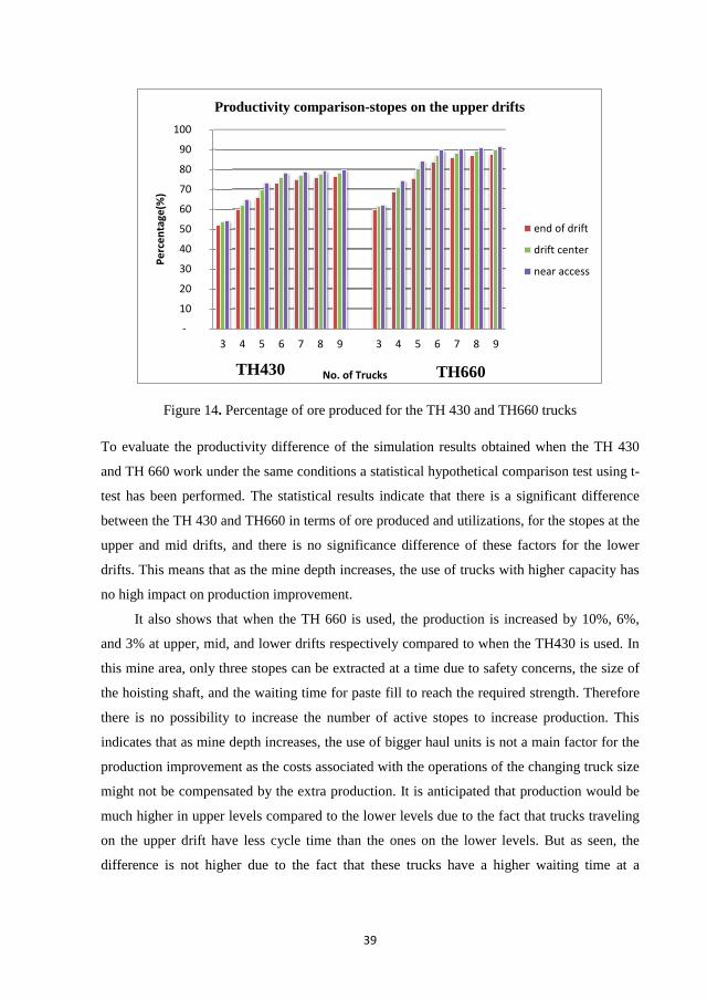
39
Figure 14. Percentage of ore produced for the TH 430 and TH660 trucks
To evaluate the productivity difference of the simulation results obtained when the TH 430
and TH 660 work under the same conditions a statistical hypothetical comparison test using t-
test has been performed. The statistical results indicate that there is a significant difference
between the TH 430 and TH660 in terms of ore produced and utilizations, for the stopes at the
upper and mid drifts, and there is no significance difference of these factors for the lower
drifts. This means that as the mine depth increases, the use of trucks with higher capacity has
no high impact on production improvement.
It also shows that when the TH 660 is used, the production is increased by 10%, 6%,
and 3% at upper, mid, and lower drifts respectively compared to when the TH430 is used. In
this mine area, only three stopes can be extracted at a time due to safety concerns, the size of
the hoisting shaft, and the waiting time for paste fill to reach the required strength. Therefore
there is no possibility to increase the number of active stopes to increase production. This
indicates that as mine depth increases, the use of bigger haul units is not a main factor for the
production improvement as the costs associated with the operations of the changing truck size
might not be compensated by the extra production. It is anticipated that production would be
much higher in upper levels compared to the lower levels due to the fact that trucks traveling
on the upper drift have less cycle time than the ones on the lower levels. But as seen, the
difference is not higher due to the fact that these trucks have a higher waiting time at a
-
10
20
30
40
50
60
70
80
90
100
3 4 5 6 7 8 9 3 4 5 6 7 8 9
Perc
enta
ge(%
)
No. of Trucks
Productivity comparison-stopes on the upper drifts
end of drift
drift center
near access
TH660TH430

40
loading point. They also travel a small portion of the ramp to reach the dumping point which
increases their time loss.
It is observed that among all the simulated scenarios, a combination of 2 trucks and a
single LHD for the upper drifts and 3 trucks and 1 LHD for the lower or mid drifts improves
the average production from 52% to 75% of planned production when the TH 430 is used, and
to 83% when the TH 660 is used. Reaching a production target of 100% proves infeasible
under the given circumstances. One possible alternative leading to production improvement
could be the additions of another ramp to minimize truck traffic, extension of the existing
shaft or adding another shaft to reduce haul distance to the existing shaft point, or considering
a different haulage method especially when the mine depth is increased.
4.2 Case study II- optimization of haulage methods based on energy requirements
In this case study, discrete event simulation and MIP are used to optimize four haulage
methods based on the energy required for each method as mine depth increases in an
Australian mine. The mine extracts copper bearing ore from an orebody striking east-west and
dipping at 70º to 75º degrees in the southerly direction. For the purposes of this study the
same orebody will be mined at three underground depth levels: 1,000 metres, 2,000 metres,
and 3,000 metres. For each depth level, four haulage options will be investigated. Each
haulage scenario will take effect from just below the crushing horizon, which will be located
at each of the three depth levels under investigation. All hauled ore will have already
undertaken a primary crushing via the underground crusher station. The method of loading
and hauling ore to transport it from the draw-point of each stope to the crusher will be carried
out via LHD units, which will be the same for each haulage option across each depth level.
The four haulage options under consideration are: diesel trucks operating on decline (inclined
at 10%)); electric trucks operating on decline (inclined at 10%); vertical shaft; decline
conveyor (inclined at 20% - 30%). The mine method used is sublevel open stoping. Stoping
conditions at a depth of 1,000 meters are generally good with stresses able to be well-
managed using standard bolting practises for both the roof and walls. This therefore allows an
open sequencing regime to be used. Stoping conditions at the 2,000-meter depth level are
such that the implementation of the stress shadowing sequence is required, due to the high
stresses that run in the north-south direction. This involves the extraction of an initial slot
perpendicular to the principle stress resulting in a redistribution of stresses around the slot
causing stopes on either side to be partly shadowed from the stress. Stopes are then
sequentially mined out from this slot toward the outer limits of the orebody. To allow for

41
greater scheduling alternatives later in the mine’s life the initial slot is placed centrally within
the orebody to gain the greatest effect from the shadowing process over as many stopes as
possible. The study is carried out using discrete event simulation and MIP to analyze the
energy requirements associated with four haulage methods as the mine depth increases.
4.2.1 Model formulation
Two models were created for the material flow at depth levels of 1000m, 2000m, and 3000m.
The first model involves diesel and electric trucks, and the second model is for the shaft and
belt conveyor. At each depth, diesel and electric trucks are loaded by loaders located at the
loading point below the crusher and they transport the ore to the stockpile near the process
plant at the mine surface. The electric trucks leave the trolley electricity line during loading
and dumping and use a small diesel motor. The total haul road distance is 10km at 10% grade.
At this grade, the load factor used for empty trucks was 0.35 and for full trucks is 0.5
(Caterpillar, 2009). A diesel oil density of 0.85kg/l was used.
For shaft modeling, a skip weight of 15 tonne was considered. This skip weight is
maintained for all mine depths with the variation of rope speed based on the required
production rate. Two and three stage shafts were used at 2,000m and 3,000m depths
respectively. Four hoist ropes of 26mm flattened strand with sheave diameter of 3.4m were
used while the efficiency of the friction hoist was estimated as 90%. The power consumption
was calculated based on the horse-power required to move the shaft up and down.
For the belt conveyor, three equal roll idlers placed at different troughing angles were
used on the carry and return side of the belt. At 1000m, the idlers placed at a 20° troughing
angle. This angle is increased to 30° when the belt operates at 2000m and 3000m depths, in
order to reduce the higher elevation of the belt when the depth increases. By using a control
system the belt speed is controlled or adjusted depending on the material flow. The variation
of the belt speed leads to a change in the power to drive the motors, which also varies the
material discharge curves. The total distance covered by the belt was 2,900km, 4,000 km and
6,000 km at 1,000m, 2,000m and 3,000m depths respectively. The power requirement for the
belt conveyor is then calculated based on elevation and friction components.
Models were developed using GPSS/H simulation language. Two models were created
whereby in each case, the variable parameters were defined. In modeling, GPSS/H uses a
process interaction approach by specifying sequences of events separated by lapses in time,
which describe the manner in which objects flow through a system. Objects may be sent
between processes that share common resources and influence the operation of all processes.

42
The representation of the objects is called transactions. The transactions compete for the use
of the available system resources. As transaction flow, they automatically queue when the
resources are not free to be used. A transaction represents the real-world system and is
executed by moving from one block to another block. Blocks are the basic structural element
of the GPSS/H simulation language. In GPSS/H there are over fifty different types of blocks
available which can be used to model complex problems (Schriber, 1989). Complete
programming codes were created and the simulation output was generated. The system was
simulated for a month, which consists of 7 working days for two shifts of 10 hours in each
day for both models. The simulation results were then used as the input in the MIP model.
The MIP model was then used to optimize the haulage operations.
4.2.2 Mixed Integer Programming (MIP) model
Optimal mine production scheduling is carried out using an MIP model to reflect and solve
the mine production scheduling problem. All extraction related activities are presented in full,
along with all formulations and constraints across the long term scheduling horizon.
Indices
The MIP model is defined in general terms using the following subscript notation.
t long-term schedule time period: t = 1, 2, 3…. T.
s long-term stope identification: s = 1, 2, 3…. S.
f fill mass identification: f = 1, 2, 3…. F.Sets
Several sets are defined which aid in the formulation of constraints.
s set of eligible long term time periods in which stope s can be in production.
t set of eligible stopes that can be in production in long term time period t.
adjs set of all stopes that are adjacent to and share a boundary with stope s.
badjf set of all stopes that are adjacent to and share a boundary with each existing fill
mass f.
tpbt set of time periods that include all periods up to the current period t.
Parameters
These parameter items represent the numeric inputs and conditions.
nt present value discount factor for time period t.
cfs undiscounted cashflow ($) from each stope s.
43
es earliest start time for stope s.
ls latest start time for stope s.
rs extraction reserve (t) for each stope s.
sct shaft/LHD/truck fleet movement capacity (t) for each time period t.
Decision variables
One binary variable was required to reflect operating conditions and ultimately perform the
scheduling task.
wst 1 if production from stope s is scheduled for time period t,
0 otherwise.
Objective function and constraints
The objective function seeks to maximize the NPV of all activities under consideration by
determining the optimal schedule within which to progress each stope through production. It
should be noted that taxation and depreciation are not included in this formulation however
they could be incorporated if necessary. The objective function is shown as equation 10.
The production scheduling model comprises numerous constraints which reflect the practical
limitations imposed by the sublevel stoping method over the long term scheduling horizon.
These constraints can be classified according to the limitations they impose on resources,
sequencing and timing. The resource constraints (11) and (12) are applicable across the long-
term horizon are Shaft/machine fleet ore capacity constraint and Non-negativity and integer
value constraint. These constraints limit the production of all development and stope
extraction ore from exceeding the shaft/LHD/truck fleet capacity in any long-term time
period, and enforce non-negativity and integer values of the appropriate variables.
The mathematical sequencing constraints that are applicable across the long term
horizon are: Stope production precedence sequencing constraint (13), Non-concurrent stope
sequencing constraint (14); Stope adjacency constraint (15), Fill mass adjacency constraint
(16); and Existing fill mass adjacency constraint (17). These constraints respectively ensure
that simultaneous production between stopes that share a common boundary does not occur.
The geotechnical stability ensures stoping activities by limiting simultaneous adjacent
production to two common boundaries before itself commencing production, and to a single
adjacent side once having completed production to become a fill mass. It also ensures that fill
mass stability of all existing fill masses by limiting exposure to a single common boundary in
each long term time period. The mathematical timing constraints that are applicable across the
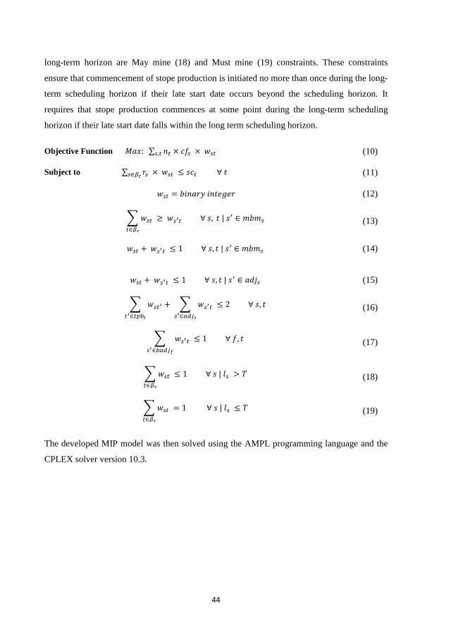
44
long-term horizon are May mine (18) and Must mine (19) constraints. These constraints
ensure that commencement of stope production is initiated no more than once during the long-
term scheduling horizon if their late start date occurs beyond the scheduling horizon. It
requires that stope production commences at some point during the long-term scheduling
horizon if their late start date falls within the long term scheduling horizon.
Objective Function : , × × (10)
Subject to × (11) = (12)
, | (13)
+ 1 , | (14)
+ 1 , | (15)
+ 2 , (16)
1 , (17)
1 | > (18)
= 1 | (19)
The developed MIP model was then solved using the AMPL programming language and the
CPLEX solver version 10.3.

45
4.2.3 Results
The initial simulation model involves diesel and electric trucks to simulate the fleet required
to achieve a monthly production target of 100,000 tonne. The results show that, although the
electric truck is 2 tonnes smaller than the diesel truck, the number of trucks required to
achieve the production target at 1,000m depth were 7 for diesel and 5 for electric. This is
because the complete cycle time of the electric truck is shorter than the diesel truck allowing
more cycles to be done within the same period of time. The simulation was repeated for the
depths of 2,000m and 3,000m and the results show that more diesel trucks are required than
electric trucks to achieve the same output.
The second model combined shaft and conveyor systems. As shown in Table 2, the
results indicated that when the depth is 1000m, a shaft system of two skips in balance each of
15 tonnes can haul the 100,000 tonnes of ore at a speed of 8.5m/s. The system is limited in
production by the rope speed. The design characteristic is based on the maximum rope speed
of 19m/s, a safety factor of 7, and a maximum skip size of 70 tonnes in order to reduce
slippage as well as avoiding exceeding the rope strength. These values were obtained based
on the characteristic curves developed by Suchard (1999) and SIEMAG-Nordberg hoisting
technology (2001). The simulation was repeatedly run with the same size of skip and variable
rope speeds. The results show that rope speeds were increased to 10m/s and 14m/s to haul
material from 2000m to 1000m, and from 3000m to 2000m respectively. It also shows that as
the rope speed increases, there is an increase in power consumption by the hoist. However the
energy consumption can be reduced when the design uses a larger skip load at a lower speed.
For this design, a skip capacity of 15 tonnes was chosen based on hoisting system type,
monthly required tonnage of 100,000 tonnes, deepest hoisting distance of 3000m and
optimum line speed.
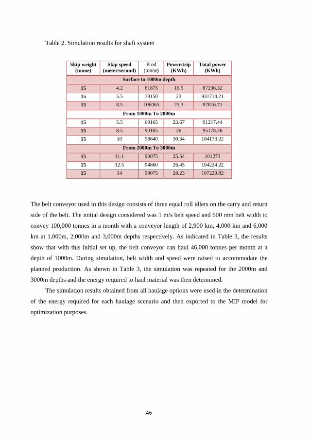
46
Table 2. Simulation results for shaft system
Skip weight (tonne)
Skip speed (meter/second)
Prod (tonne)
Power/trip (KWh)
Total power (KWh)
Surface to 1000m depth
15 4.2 61875 16.5 87236.3215 5.5 78150 23 931714.2115 8.5 106065 25.3 97816.71
From 1000m To 2000m
15 5.5 69165 23.67 91217.4415 8.5 90105 26 95178.2615 10 98640 30.34 104173.22
From 2000m To 3000m
15 11.1 90075 25.54 10127315 12.5 94860 26.45 104224.2215 14 99075 28.23 107229.82
The belt conveyor used in this design consists of three equal roll idlers on the carry and return
side of the belt. The initial design considered was 1 m/s belt speed and 600 mm belt width to
convey 100,000 tonnes in a month with a conveyor length of 2,900 km, 4,000 km and 6,000
km at 1,000m, 2,000m and 3,000m depths respectively. As indicated in Table 3, the results
show that with this initial set up, the belt conveyor can haul 46,000 tonnes per month at a
depth of 1000m. During simulation, belt width and speed were raised to accommodate the
planned production. As shown in Table 3, the simulation was repeated for the 2000m and
3000m depths and the energy required to haul material was then determined.
The simulation results obtained from all haulage options were used in the determination
of the energy required for each haulage scenario and then exported to the MIP model for
optimization purposes.

47
Table 3. Simulation results for belt conveyor
Belt width(mm)
Prod (tonnes)
Capacity t/hr
Belt speed (m/s)
Power/trip ( KWh)
Total Power (KWh)
At 1000m600 46135 79 1 119 78430.07650 55339 84 1.2 143 94208.17750 91006 138 1.3 235 154974.32
900 108811 165 1.3 283 186628At 2000m
600 44027 152 1.3 304 333914.27650 50196 178 1.4 357 391666.62750 58064 191 1.5 383 420617.09900 108819 340 1.6 681 749210.43
At 3000m600 71868 339 1.6 780 857765.23650 83952 396 1.6 99 1001825.8750 96036 453 1.6 1043 1146986.06900 100700 475 1.6 1092 1200871.32
Construction of all MIP models for the purpose of optimal production scheduling
(maximize NPV) took place using a Mathematical Programming Language (AMPL), based on
the operating costs and extrapolated simulation results then solved using CPLEX 10.3.
Production scheduling took place at monthly intervals and was limited to 180 periods (15
years). The energy costs were determined based on operating NPVs and energy cost per tonne
of ore for each haulage option for the current and future energy prices. As shown in Figure 15,
diesel trucks have higher energy costs with increasing depth for both energy price scenarios
compared to other haulage options. It shows that the energy costs for diesel trucks are
responsible for 38.2%, 46.8% and 63.1% of operating costs at the 1,000, 2,000 and 3,000
meter depth levels respectively at the current energy price. At three times the current energy
prices, energy costs at the 1,000, 2,000 and 3,000 meter depth levels for diesel truck haulage
significantly increase to 64.9%, 72.5% and 83.7% of operating costs respectively. The lowest
energy cost component increase is observed to be for the shaft haulage system. It shows that
for shaft haulage at the 1,000, 2,000 and 3,000 meter depth levels at the current energy price,
energy costs only account 10.8%, 13.0% and 15.4% of operating costs. At three times the
current energy prices, energy costs at the 1,000, 2,000 and 3,000 meter depth levels for shaft
haulage account for 26.6%, 30.9% and 35.4% of operating costs respectively.

48
Figure 15. Energy & non-energy cost components of the operating cost as a percentage of total operating costs at current and three times the current energy prices
Since it is recognized that the ore haulage process is one of the most energy-intensive
activities in a mining operation and is thus one of main contributors to operating cost, it is
therefore appropriate to analyze the haulage cost component of the operating cost as a
percentage of the total operating cost. As can be seen in Figure 16 across all cases, the results
show an increasing trend for the energy cost component of the haulage cost to increase in
combination with the increase in depth with higher costs on diesel trucks and lower costs on
the shaft system.
0%
10%
20%
30%
40%
50%
60%
70%
80%
90%
100%
Dies
el T
ruck
(100
0m)
Dies
el T
ruck
(200
0m)
Dies
el T
ruck
(300
0m)
Elec
tric
Tru
ck (1
000m
)El
ectr
ic T
ruck
(200
0m)
Elec
tric
Tru
ck (3
000m
)
Shaf
t (10
00m
)Sh
aft (
2000
m)
Shaf
t (30
00m
)
Conv
eyor
(100
0m)
Conv
eyor
(200
0m)
Conv
eyor
(300
0m)
Perc
enta
ge o
f Ope
ratin
g Co
st (%
)
Haulage Method (Depth)
Energy & Non-energy Cost Components as a Percentage of Operating Cost at
Current Energy Price
Non-Energy Component of Operating Cost
Energy Component of Operating Cost
0%
10%
20%
30%
40%
50%
60%
70%
80%
90%
100%
Dies
el T
ruck
(100
0m)
Dies
el T
ruck
(200
0m)
Dies
el T
ruck
(300
0m)
Elec
tric
Tru
ck (1
000m
)El
ectr
ic T
ruck
(200
0m)
Elec
tric
Tru
ck (3
000m
)
Shaf
t (10
00m
)Sh
aft (
2000
m)
Shaf
t (30
00m
)
Conv
eyor
(100
0m)
Conv
eyor
(200
0m)
Conv
eyor
(300
0m)
Perc
enta
ge o
f Ope
ratin
g Co
st (%
)
Haulage Method (Depth)
Energy & Non-energy Cost Components as a Percentage of Operating Cost at Three Times
Current Energy Price
Non-Energy Component of Operating Cost
Energy Component of Operating Cost

49
Figure 16. Energy & non-energy cost components of the haulage cost as a percentage of total haulage costs at current and three times current energy prices
Diesel truck haulage generally offers greater operational flexibility, its high energy-intensity
results in a rapid reduction in its financial viability with increasing depth. Shaft haulage was
observed to have lower energy cost increase at the 1,000, 2,000 and 3,000 meter depth levels
for both energy price scenarios. An analysis of these results clearly shows that in an era of
increasing energy prices and the increased need to mine at greater depths, only those haulage
methods with lower energy requirements will remain viable. The implementation of lower
energy-intensive haulage methods often means a greater initial capital cost is required. In
addition to this they generally offer less flexibility. This in turn emphasizes the value of the
mine planning process with the aid of discrete event simulation and MIP to guide decision
making to the operations at great depth.
0%
10%
20%
30%
40%
50%
60%
70%
80%
90%
100%
Dies
el T
ruck
(100
0m)
Dies
el T
ruck
(200
0m)
Dies
el T
ruck
(300
0m)
Elec
tric
Tru
ck (1
000m
)El
ectr
ic T
ruck
(200
0m)
Elec
tric
Tru
ck (3
000m
)
Shaf
t (10
00m
)Sh
aft (
2000
m)
Shaf
t (30
00m
)
Conv
eyor
(100
0m)
Conv
eyor
(200
0m)
Conv
eyor
(300
0m)
Perc
enta
ge o
f Hau
lage
Cos
t (%
)
Haulage Method (Depth)
Energy & Non-energy Cost Components as a Percentage of Haulage Cost at
Current Energy Price
Non-Energy Component of Haulage Cost
Energy Component of Haulage Cost
0%
10%
20%
30%
40%
50%
60%
70%
80%
90%
100%
Dies
el T
ruck
(100
0m)
Dies
el T
ruck
(200
0m)
Dies
el T
ruck
(300
0m)
Elec
tric
Tru
ck (1
000m
)El
ectr
ic T
ruck
(200
0m)
Elec
tric
Tru
ck (3
000m
)
Shaf
t (10
00m
)Sh
aft (
2000
m)
Shaf
t (30
00m
)
Conv
eyor
(100
0m)
Conv
eyor
(200
0m)
Conv
eyor
(300
0m)
Perc
enta
ge o
f Hau
lage
Cos
t (%
)
Haulage Method (Depth)
Energy & Non-energy Cost Components as a Percentage of Haulage
Cost at Three Times Current Energy Price
Non-Energy Component of Haulage Cost
Energy Component of Haulage Cost

50

51
5. DISCUSSION
The results of the research work have been discussed based on the research questions
highlighted early.
Research question 1: What are the drawbacks of using analytical methods on
underground equipment selection?
The first research question is answered by paper A and B, and a literature review in chapter 3.
For many years, analytical methods have been widely used in equipment selection for both
open pit and underground operations. The method is used to evaluate the load and haul
equipment, which operates in the haulage network which comprises many structures such as
ramps, crosscuts, decline, inclines and levels. When equipment enters this system, it behaves
randomly due to the variation of these working conditions. The existence of many uncertain
operational elements and the random behavior of the system make haulage selection less
accurate when using analytical calculation since the calculation will not explicitly
acknowledge the uncertainty and randomness. As seen in the literature review, the analytical
approach is also limited in modeling complex operations, has low flexibility and cannot
predict the future operations. Most analytical methods require a small amount of data because
the method tends to be a fairly simple description of the system. The use of analytical
methods can still be successfully used in small mining operations, which have less
uncertainty, but most large mining operations need methods which will involve randomness
and can handle complexity.
Research question 2: Is discrete event simulation a suitable tool for equipment selection
and analyzing the performance of underground haulage systems?
The second research question is answered by paper A and B.
As the underground haulage operations are of a dynamic and stochastic nature, the discrete
event simulation approach was considered to be the most appropriate technique to deal with
such operations. Discrete event simulation is known for having the advantage of providing
more accurate accounting for real world uncertainty and diversity. Furthermore it
acknowledges the variability of the interdependent components within the operations.
Discrete event simulation has been improved in parallel with the rapid development of
computer technology. With more powerful, flexible and user-friendly software development,

52
discrete event simulation will be a useful tool for mine planning, system design and
operations analysis in the mining industry. As seen in Case Study One and Two, the use of
simulation methods will also allow much quicker evaluation of equipment selection for
different haulage options and provide a viable alternative to analytical methods as it reduces
the subjectivity associated with operational systems.
As can be seen in paper A and B, the tool is suitable when;
Enough data is available to make better use of the randomness
Carefulness should be taken in the choice of discrete event simulation software
Fitting of data into statistical distributions should be done correctly
Discrete event simulation is incorporated with economic models to assess the
economic impact of mining operations.
Research question 3: Is it possible to combine discrete event simulation and mixed
integer programming to optimize underground haulage operations?
The third research question is answered by paper C.
Discrete event simulation is a suitable tool to solve problems that involve randomness where
the flexibility of the system significantly affects the behavior of the operations. Discrete event
simulation has gained increased attention as a technique for analyzing mining operations and
modifying or improving existing ones. As described in Case Study Two, discrete event
simulation can be used to study the behavior of mining operations and make predictions
before a new system is implemented. However, discrete event simulation technique is not
suitable for directly solving complex optimization problems like mine planning. The
technique can be combined with MIP to provide a feasible solution and increase an
understanding of and increase the flexibility of the operations. The combined tool can also be
used in:
Studying economic analysis models to improve understanding of the behavior of
various systems and reduce risk when selecting the underground haulage operations.
Decision-making on optimization problems with the inclusion of economic objectives
such as cost minimization or maximization of contribution to the profit.
Increasing the viability of the mine plans prior to execution, allowing equipment
utilization analysis, and making possible the analysis of several scenarios within a
short time interval.

53
6. CONCLUSIONS
Based on the conducted research the following conclusions have been made.
General conclusions
When the hauling systems involve random behavior, the use of analytical methods
becomes less accurate when used to model such operations. In such cases, methods
such as discrete event simulation can be implemented as they have advantage of more
accurate accounting for the real world uncertainty and diversity in operations.
To increase efficiency, the use of simulation for mine equipment selection can be
combined with economic analysis models to improve understanding of the behavior of
various systems. This provides a more feasible solution for complex optimization
problems, and hence increases the possibility to improve both the productivity and the
flexibility of the production operations and reduces risks when selecting the
equipment.
Discrete event simulation combined with mixed integer programming provides mining
operations with a preliminary assessment of the energy costs associated with various
haulage methods in the context of an increase in mine depth. This can aid the decision-
making process with regard to future deeper underground mining.
Conclusions from case studies:
The results from Case Study one show that, among all the simulated scenarios, a
combination of 2 trucks and a single LHD for the upper drifts and 3 trucks and 1 LHD
for the lower or mid drifts improves the average production from 52% to 75% of
planned production when the TH 430 is used, and 52% to 83% when the TH 660 is
used
The Case Study two shows that, the energy costs for diesel trucks are higher compared
to other haulage options. These account for 38.2%, 46.8% and 63.1% of operating
costs at the current energy price, and 64.9%, 72.5% and 83.7% of operating costs at
the future energy prices at the depth levels of 1,000, 2,000 and 3,000 meters
respectively.

54
The energy cost is observed to be lower for the shaft haulage system. It accounts for
10.8%, 13.0% and 15.4% of operating costs at the current energy price, and for 26.6%,
30.9% and 35.4% of operating costs at the future energy price at the 1,000, 2,000 and
3,000meter depth levels respectively.
Haulage costs were also analyzed as a percentage of the total operating cost for all
options. The results show that diesel truck haulage is substantially higher compared to
other haulage options with the lowest energy cost on the shaft haulage system.

55
7. FUTURE WORK
Based on the conducted research, future study in this field may include the following:
Rail transportation: This is one of most energy-efficient modes of transportation in
underground mines with high tonnage production per shift and long haulage distances.
Metal price variations: Deposits are usually analyzed by converting the metal grades
into revenues and classifying the resource blocks by value according to predictions
about metal prices. As mines continue to operate, metal price variations will occur and
the maximization of the cash flow will need the variation of these values to improve
the planning accuracy.
Variation of the cut of the grade: this will cause the grade of each block to vary from
its estimate, which may result in reduction of or addition to the production rate.
Also the work could be incorporated into the methodology developed to evaluate the
impact of incorporating the risk directly related to each component by applying the
individual discount rates of various components to the cashflow.
Gas emissions: The energy cost is one of the largest components of the total operating
costs in underground mining operations. In underground mines, higher gas emissions
increase the ventilation cost. Therefore future studies may include estimation of gas
emissions on each haulage options.
Sensitivity analysis: Conditional simulation to measure the sensitivity of the
parameters involved in the selection of haulage methods for deep underground
operations.

56
57
REFERENCE
1. Alford, C., 1995, Optimisation in underground mine design, 25th Int. APCOM.
Symposium, Australasian Instit. Mining and Metallurgy: Melbourne, pp. 213-218.
2. Almgren, T. 1994, An approach to long range production and development planning with application to the Kiruna mine, Sweden. Doctoral thesis:143D Luleå University of Technology, Luleå, Sweden.
3. Ataee-Pour, M., 2005, A critical survey of existing stopes layout optimisation techniques, J. Mining. Science, Springer: New York, pp. 447-466.
4. Atkinson, T., 1992, Selection and sizing of excavating equipment, in SME Mining Engineering Handbook, H.L Hartman, 2nd ed., Littleton CO SME, pp1311-1333.
5. Banks, J., 2000, Introduction to simulation, Proceedings of the winter simulation, Orlando, pp. 9-16.
6. Banks, J., Carson, J.S., Nelson, B.L., and Nicol, D.M., 2010, Discrete event System simulation, Pearson Education, New Jersey.
7. Basu, A.J. and Baafi E.Y., 1999, Discrete event simulation of mining systems, Current practice in Australia, International Journal of Mining Reclamation and Environment,Vol. 13, No. 2, pp. 79-84.
8. Beerkircher, G., 1989, Mine hoists: Underground mining methods handbook, in SME,chap. 5.5, USA, pp. 1386-1403.
9. Brazil, M., and Thomas, D.A., 2004, Network optimisation for the design of underground mines, InterScience, John Wiley and Sons Inc. New Jersey.
10. Brucker, D., 1975, Faster and deeper: the saga of the times in hoisting, ASEA Info. No. AS100-104E, Montral, Quebec.
11. Carlyle M., and Eaves, B.C., 2001, Underground planning at Stillwater Mining Company, Interfaces. Springer: New York, pp. 50-60.
12. Caterpillar, 2001, A reference guide to Mine Machine Applications. Peoria, IL, Caterpillar.
13: Caterpillar, 2009, Caterpillar Performance Handbook, Edition 39, Caterpillar Inc., Peoria, IL.
14. Chanda, E.C.K., 1990, application of integer programming and simulation to production planning for stratiform ore body, Mining Science Technology, 11:2, pp. 165-172.
15. Edwards, F.A, 1988, A systematic approach to the design of the mine shaft hoisting system, Proceeding International Conference on hoisting men, materials, and minerals,Canadian Institute of Mining and Metallurgy, Vol 1, pp. 39-73.
16. Elbrond, J., 1964, Capacity calculations at LKAB, Kiruna, APCOM Proceedings, Denver, CO, pp. 683-690.

58
17. Ercelebi, S.G., and Kirmanli, C., 2000, Review of surface mining equipment selection techniques’, Mine Planning and Equipment Selection, Ed Pasamehmetoglu. Et al. Balkema, Rotterdam, pp 547-553.
18. Fenner Dunlop, 2009, Conveyor Handbook, Australia.
19. Fiorini, M.M., Franzese, L.A.G., Bianchi, T.J., Ezawa, L., Pinto, L.R., and De Miranda, J., Gilberto, 2008, Concurrent simulation and optimization models for mining planning. Paper presented at the WSC’08: Proceedings of the 40th Conference on Winter simulation, Miami, Florida. 759-767.
20. Goodyear and Rubber company, 1976, Handbook of Conveyor &Elevator belting, Akron, Ohio 44316, USA, Chap. 6, pp. 1-8.
21. Ghosh, B.N., 1982, scientific methods and social research, New Delhi, Sterling publishers Pvt.Ltd.
22. Greberg, J. and Sundqvist, F., 2011, Simulation as a tool for mine planning, In Proceedings of Second International Future Mining, Melbourne, pp. 273-278.
23. Hager, M., and Hintz, A., 1993, The Energy-Saving design of belts for long conveyor systems, Bulk Solids Handling, 13:4, pp. 749-758.
24. Hartman, H.L, 1987, Introductory mining Engineering, John Wiley and Sons, New York, USA.
25. Harmon, J.H., 1973, Hoist and hoisting systems, in SME, Chap 15. SME-AIME, New York, pp. 15-59.
26. Harrison, J. and Sturgul, J.R., 1989, GPSS Computer simulation of equipment requirements for the iron duke mine, Second large open pit mining conference, Melbourne, Vie., AusIMM, pp. 133-136.
27. Hiltermann, J., Lodewijks, G., Schott, D.L., Rijsenbrij, J.C., Dekkers, J.A.J.M. and Pang, Y., 2011, A Methodology to Predict Power Savings of Troughed Belt Conveyors by Speed Control, Particulate Science and Technology, International Journal of Mining Reclamation and Environment, 29:1, pp. 14-27.
28. Kecojevic, V., and Komljenovic, D., 2010, Haul truck fuel consumption and CO2 emission under various engine load conditions. Mining Engineering. 62:12, ProQuest Central, pp. 44-48.
29. Ketelaar, J.P.I and Davidson, P.J., 1995, Improving the efficiency of conveyors used for the transport of minerals in underground and surface mines, Mining Tech, 77:88.
30. Knights, P.F. and Bonates, E. J.L., 1999, Applications of discrete mine simulation modeling in South America’, International Journal of Mining Reclamation and Environment, 13:2, pp. 69-72.
31. Konyukh, V., Galiyev, V., and Li, Z., 1999, Mine simulation in Asia’, International Journal of Mining Reclamation and Environment, Vol. 13, No. 2, pp. 57-67.
32. Kothari, C.R. 2004, Research methodology: Methods and techniques, New age international publishers, New Delhi, India.
59
33. Law, A.M., and Kelton, W.D., 1991, Simulation Modeling analysis, Second edition, McGraw-Hill, New York.
34. Lerchs, H and I.F. Grossmann 1965, Optimum design of open pit mines. Trans. Canadian Institute of mining, Vol 68, pp 17-24.
35. Littler, A., 2000, Sand and gravel production, institute of Quarrying.
36. Lizotte, Y. and Bonates, E., 1987, Truck and shovel dispatching rules assessment using simulation, International Journal of Mining Science. Tech. 5, pp. 45-58.
37. Morrison, D.M., 1996, Deep hard rock mining: The future, CIM Bulletin, vol. 89, no. 10000, pp 46-51.
38. Mutagwaba, W. and Durucan, S., 1993, Object-oriented simulation in mine transportation design, Mine Mechanization and Automation, G.Almgren, U. Kumar and N. Vagenas (eds), Rotterdam:Balkema, pp. 591-600.
39. Murata, T, 1989, Petri Nets: Properties, Analysis and Applications. Proceedings of the IEEE, 77(4): pp 541–580.
40. McIsaac, G., 2005, Long-term planning of an underground mine using mixed-integer linear programming, CIM Bulletin, Canad. Inst. Mining. Metal. Petroleum, Westmount.
41. Nehring, M., Topal, E. and Little, J., 2010, A new mathematical programming model for production schedule optimization in underground mining operations. J. South. African Inst. Mining. Metall, 110:8, pp. 437-446.
42. Newman, A., Kuchta, M., Martinez, M., 2007. Long- and short-term production scheduling at LKAB’s Kiruna mine. In Weintraub, A., Romero, C., Bjørndal, T., Epstein, R. (eds) Handbook on Operations Research in Natural Resources. Springer, New York, pp. 1205–1218.
43. Nogueira, J.A., 1984, Controle de Equipamentos e Dispatching’. Seminario O Computador e sua Applica ão no Setor Mineral, Belo Horizonte, Brazil, pp. 89-96.
44. Oberndorfer, T. 1992, Mining method selection techniques - requirements for successful solutions, in Y. Kim, ed., 23rd application of computers and operations research in the mineral industry, Society for Mining, Metallurgy, and Exploration, Littleton, Colorado, pp. 145-155.
45. Panagiotou, G.N., 1999, Discrete mine system simulation in Europe, International Journal of Mining Reclamation and Environment, 13:2, pp. 43-46.
46. Raj, M.G., Vardhan, H. and Rao, Y.V., 2009, Production optimization using simulation models in mines: a critical review, International Journal of Operational Research, 6:3, pp. 330-359.
47. Rist, K., 1961, The solution of a transport problem by use of Monte Carlo Technique, paper presented at APCOM 1, Arizona, USA.
48. SIEMAG-Nordberg hoisting technology, 2001, Special topic: Design of hoisting systems, SIEMAG-Nordberg, Milwaukee.
60
49. Singh, S.P., 1993, Prediction and determination of explosive induced damage, rock fragmentation by blasting, Rossmanith (ed.), Balkema, Rotterdam, pp. 183-192.
50. Singh, K.H and Rajala, L.H, 1981, Falconbridge introduces advanced technology to deep mining, Canadian Institute of Mining and Metallurgy Bulletin, pp. 75-84.
51. Schulz, S.H, 1973, Shaft installations of high winding capabilities, Proceeding International Conference on hoisting men, materials, and minerals, South Africa Institute of mechanical engineers, pp. 169-176.
52. Scott, F.E., 1982, Diesels underground overcoming a bad image, Coal mining and processing, Vol. 19:8, pp. 45-51.
53. Schriber, T., 1989, Perspectives on simulation using GPSS, in Proc. Winter. Simulation, M. Abrams, ed., Society of Computer Simulation, Publisher, San diego, CA.
54. Sturgul, J.R., 1999, Discrete mine system simulation in the United States, International Journal of Mining Reclamation and Environment,13: 2, pp. 37-41.
55. Sturgul, J.R, 1995b, History and annotated bibliography of mine systems simulation, department of metallurgy and mining, University of Idaho, third printing, USA.
56. Sturgul, J.R and Jacobson, W.L., 1994, A simulation model for testing a proposed mining operation: Phase 1, Mine Planning and Equipment Selection, Pasamehmetoglu et al. ed (Rotterdam: Balkema), pp. 281-287.
57. Sturgul, J.R, 1996, Annotated bibliography of mine systems simulation (1961-1995), International symposium on mine simulation via the internet.
58. Sturgul, J.R., and Singhal, R., 1988, Using the personal computer to simulate mining operations, in Proc Computer. Applic. Mineral. Industry (CAMI), Laval University, Quebec city, Balkema, Publisher, Rotterdam, pp. 439-442.
59. Sweigard, R., 1992, Materials handling: Loading and haulage. In SME Mining Engineering Handbook, 2nd ed. Edited by H.L Hartman. Littleton, CO: SME.
60. Swinderman, R.T., 1991, The conveyor drives power consumption of belt cleaners. , Bulk Solids Handling, 11, pp. 487.
61. Suchard, G., 2003, Koepe/Friction hoists-Hard rock miner’s Handbook rules of thumbs, by J.D.I Vergne, McIntosh Engineering, Tempe, Arizona.
62. Turner, R.J., 1999, Simulation in the mining industry of South Africa, International Journal of Mining Reclamation and Environment, 13:2, pp. 47-56.
63. Thomas, N., Gregg, A.J, and Hartman, H.L., 1987, Comparative performance study of diesel and electric face-haulage vehicles. Int. J. Mining. Geologic. Eng., 5, pp. 405-417.
64. Tudhope, I.S.D, 1973, Multi-rope winders for high capacity hoisting, Proceeding International Conference on hoisting men, materials, and minerals, South Africa Institute of mechanical engineers, pp. 152-168.
65. Topal, E., 2008, Early start and late start algorithms to improve the solution time for long-term underground mine production scheduling, J. South. African Inst. Mining. Metall.

61
66. Trout, L.P. 1995, Underground mine production scheduling using mixed integer programming. 25th international application of computer operation research in mineral industry (APCOM) Symposium. Proceedings, Brisbane, Australia, pp. 395-400.
67. Wilke, F.L., 1970, Simulation studies of computer controlled traffic underground in large coal mines, 9th International Symposium on Decision Making in the Mineral Industry, Can 1MM, sp. 12, pp. 344-351.
68. Wilker, F.L., 1987, Recent methodological trends in operations research and computing as applied to mining problems. In Proc. APCOM Symp., 20th (S. Af. Inst. Min. Metal., Johannesburg), Vol. 1, pp 109-113.
69. Winston, W.L., and Goldberg, J.B., 2004, Operations research: applications and algorithms, Thomson: Belmont, 2004.
70. White, J.P., and Olson, J.W., 1986, Computer-based dispatching in mines with concurrent operating objectives. Mining Engineering, 38:11, pp 1045-1054.
71. Xu, G. and Dong, Z., 1974, Mathematical simulation of the mining process at Mines, Practice and Knowledge of mathematics, Vol. 4, pp. 26-37 (in Chinese).
72. Yardley, E.D and Stace, L.R., 2008, Belt conveying of minerals, Woodhead publishing and CRC Press, USA.
73. Yuriy, G. and Vayenas, N., 2008, Discrete-event simulation of mine equipment systems combined with a reliability assessment model based on genetic algorithms’, International Journal of Mining Reclamation and Environment, 22:1, pp. 70-83.
74. Zhao, R., Suboleski, S. 1987, Graphical simulation of continuous miner production systems, APCOM 87: Proceedings of the 12th International symposium on the application of computers and mathematics in the mineral industry.


APPENDED PAPERS

PAPER A
Optimization of Truck-Loader haulage system in an underground mine: A simulation approach using SimMine
A.J. Salama and J.Greberg, Optimization of Truck-Loader haulage system in an underground mine: A simulation approach using SimMine. In the proceedings of the 6th International Conference and Exhibition on Mass Mining, Sudbury, ON, Canada, 10-14, June, 2012.

Optimization of Truck-Loader haulage system in an underground mine: A simulation approach using SimMine
Abubakary .J. Salama, PhD student, Luleå University of TechnologyJenny Greberg, Assistant Professor, Luleå University of Technology
Abstract
In underground mining, the truck-loader haulage system involves mucking of the material from the working face and transporting it to the dumping point where it is reloaded into trucks for further transportation. In some cases, trucks can be loaded directly at the working face or at a dumping point. Due to a limited size of the drifts and the ramps used in transporting material, the size of the haulageequipment is an important factor to consider when seeking to optimize the haulage system. This paper studies the haulage system of a mine which operates a fleet of three Load-Haul-Dump (LHD) machines and three dump trucks, using SimMine simulation software. Its aim is to evaluate the effect of increasing the number of trucks on the overall mine throughput. The results indicated that the capacity of the existing loading equipment does not match the number of trucks; this affects the haulage system and the mine production. The study resulted in the recommendation to increase the fleet of dump trucks.
Biography
Salama A.J Holds a Master’s degree in Mining Engineering from Paris School of Mines in France. His mining experience is in Sub level stope mining operations. Currently he is pursuing a PhD in Mine Production at Luleå University of Technology. His research interest is production simulation and optimization with respect to mining at great depth.
Greberg J. Holds a PhD-degree from Lund University of Techlonolgy in Sweden. Before joining Luleå University of Technology as an assistant Professor, she worked in the Aerospace industry and as mining consultant. Currently she is the head of division of Mining and Geotechnical Engineering at the LuleåUniversity.

1. Introduction
In underground mining, a Truck-Loader haulage system is used to transport fragmented material from the production area to the desired location. The haulage system depends on the mining method employed. When a mine uses the sublevel open stope method, the truck-loader haulage system involves mucking material from the mine face, transporting it to loading areas where it is reloaded into trucks for transportation to the mine surface (Sweigard, 1992). Trucks can be loaded directly at the face or at separate loading areas. In hard rock mines, ramps size cannot accommodate more than one vehicle traveling in opposite direction at a time (Sabuncuoglu, 1992). Due to the limited size of drifts and ramps used as haul ways, the selection of effective loading and hauling machines becomes an important factor to consider if a mine wishes to optimize its haulage system. This paper presents a simulation study of the truck-loader haulage system with a view to optimizing the mine’s fleet.
2. Simulation in Mining operations
Simulation is the imitation of the real world processes or systems over time (Banks, 1999). The ultimate goal is to model a real life system with the aim of understanding the behaviour of the system by evaluation various strategies within the limits imposed by a criterion or set of criteria for the operation of the systems(Saiang, 2008). Examples of Systems that can be simulated include transportation logistics, business processes, mining operations, emergency response systems etc. Simulations can apply a number of rules and procedures, thereby increasing the understanding of the interaction between variables and their importance in the system performance and suggesting possible system modifications (Banks, 2000).
In mining operations, simulation methods can be used to simulate various systems and study various issues such as fleet requirements, the flow of hauling machines, and mine planning, with the aim of optimizing, improving, and analyze existing and future systems. Simulations can also be used to makecritical decisions and to increase the overall understanding of the mining system (Sturgul & Li, 1997).
A large number of simulation languages, including GPSS/H, SLAM, ARENA, etc, are available and widely used in mining operations, making the traditional methods such as manual calculations less common when solving complex problems. The use of simulation tools increases the understanding of the system performance and the interaction of the many variables involved. Most simulation studies applied to mining operations have focused on selected parts of the mining operation, such as development loading,transport and processing of material. More recent studies have attempted to simulate larger parts of the mining system or even a complete mine (Greberg & Sundqvist, 2011).
3. The simulation study
This paper presents the case study of a deep underground mine. The mine is currently operating at 1300m depth, but recent exploration shows that the ore body extends beyond 2000m. Underground levels are accessed by a vertical shaft and two ramps; the vertical shaft extends about 1000m below the surface.Below 1000m depth, there is only one ramp with a single lane extended. Materials from the lower levels are transported by dump trucks to the lowest tipping point of the shaft and then hoisted to the surface by skips.
The ore body is divided into zones A, B, and C, with an average thickness of 3.5m, 3.1m, and 2.4m respectively. The mine uses four different mining methods: sublevel open stoping in zones A and B; drift and fill mining in zone C; narrow vein mining in zone C; Alimak mining in zones A and B. This paper focuses on the sublevel open stoping mining used in zone A. In this method, top and bottom accesses are mined to reach the sublevel open stope. Slots are formed by conventional raises and occasionally drop raises. Stopes are drilled using both up and down holes as shown in Figure 1. Upholes are drilled up from the lower level to half the distance between the two drives (10m); downholes are drilled down from the
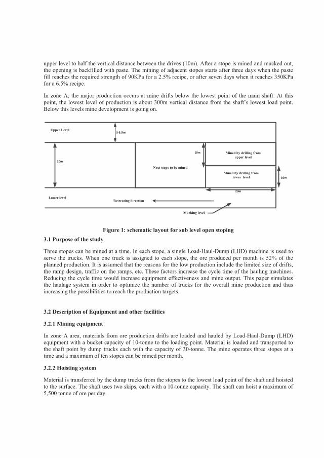
upper level to half the vertical distance between the drives (10m). After a stope is mined and mucked out, the opening is backfilled with paste. The mining of adjacent stopes starts after three days when the paste fill reaches the required strength of 90KPa for a 2.5% recipe, or after seven days when it reaches 350KPa for a 6.5% recipe.
In zone A, the major production occurs at mine drifts below the lowest point of the main shaft. At this point, the lowest level of production is about 300m vertical distance from the shaft’s lowest load point.Below this levels mine development is going on.
Next stope to be mined
Retreating direction
Upper Level
Lower level
10m
10m
20m
3-3.5m
Mined by drilling from upper level
Mined by drilling from lower level
20m
Mucking level
Figure 1: schematic layout for sub level open stoping3.1 Purpose of the study
Three stopes can be mined at a time. In each stope, a single Load-Haul-Dump (LHD) machine is used to serve the trucks. When one truck is assigned to each stope, the ore produced per month is 52% of the planned production. It is assumed that the reasons for the low production include the limited size of drifts,the ramp design, traffic on the ramps, etc. These factors increase the cycle time of the hauling machines.Reducing the cycle time would increase equipment effectiveness and mine output. This paper simulatesthe haulage system in order to optimize the number of trucks for the overall mine production and thus increasing the possibilities to reach the production targets.
3.2 Description of Equipment and other facilities
3.2.1 Mining equipment
In zone A area, materials from ore production drifts are loaded and hauled by Load-Haul-Dump (LHD)equipment with a bucket capacity of 10-tonne to the loading point. Material is loaded and transported to the shaft point by dump trucks each with the capacity of 30-tonne. The mine operates three stopes at a time and a maximum of ten stopes can be mined per month.
3.2.2 Hoisting system
Material is transferred by the dump trucks from the stopes to the lowest load point of the shaft and hoisted to the surface. The shaft uses two skips, each with a 10-tonne capacity. The shaft can hoist a maximum of 5,500 tonne of ore per day.

3.2.3 Ramp configuration
The ramp has an average width of 5.5m, and a height of 5m, with grades ranging from 11% to 15%. The ramp length in deeper levels where development is still going on is estimated by using the standard Euclidean length:
)11( 2),( mZZL kllk
where L (k,l) stands for the length of the ramp link, |Zl – Zk| represents the difference in vertical elevation between the two end points of the link, k and l are two end points of the link, and m is the ramp grade.
4. Data Collection
At a mine visit in August 2011, data were collected for 14 days on the dayshift and 6 days on the nightshift. There were constraints on acquiring data during the nightshift, as it was more difficult to access the mine at that time. Data collected and which used in the simulation model include truck cycle times, LHD cycle times, ore production, haul route profiles, rock overbreaks, and machine settings.
4.1 Truck cycle time
Truck cycle time includes spotting or truck maneuvering time, loading time, travelling time when fully loaded, dumping time, and travelling time back to the loading point. A cycle time survey was done by following the truck from the loading point to the shaft bottom point. The survey found that the time varies from one run to another: for example, the first cycle can last 19 minutes, the second can take 19.8 minutes, and so on. Many factors contribute to these variations, which include payload variations, ramp curvatures, operator efficiency, ramp grade, lighting, etc. (B. Morgan, 1994). A total of 57cycles for the dayshift and 33 for the nightshift were recorded from three working drifts.
4.2 LHD loading timeLHD-machines are used to load the trucks at the loading bay as shown in Figure 2. When there is no truck to load, LHDs haul the material and dump it on a stockpile. Loading time per pass includes bucket travelling time when empty, digging time, bucket travelling time when loaded, and loading time. The study recorded a total of 43 cycles for the dayshift and 29 cycles for the nightshift in different loading locations.
4.3 Planned and actual production The ore mucked out from each stope is transported to the bottom point of the shaft and then hoisted to the surface. The amount of ore hauled from the sub level stopes in zone A is recorded at the end of each shift. The study found that the amount of ore produced per month is approximately 52% of the mine’s production target when stopes located at the upper drifts are in operation. The percentage of ore produced is expected to fall as the mine depth increases.
4.4 Face profile
A stope pattern of 20m by 10m is blasted per round from the end of the drifts back to the access. Face profiles of the openings are shown in Table 1. The footwall access at the shaft tipping point is high enough to allow trucks to tip the material. The ramp has several refuge chambers which allow vehicles to give way to each other.

Table 1: Face profiles for different openings
Face profileDescription Width (m) Area (m2)
Ore drifts Production drifts 3.5 10.5Main Levels Footwall access 5.5 30.25
Ramp Fleet hauling tunnel 5.5 27.5Access Crosscut between ramp and drift 4.5 20.25
4.5 Shift schedules
The mine operates two shifts per day of 10 hours each. The dayshift starts at 6:00a.m and ends at 4:00 p.m., with two hours for a meal break and shift preparations. The nightshift starts at 6:00 p.m. and ends at 4:00 a.m., also with two hours for shift preparations and a meal break. The blasting is conducted once a day during the shift change. This makes the effective working time 16 hours a day, resulting in 80% shift utilization. The interaction of dump trucks with other mine vehicles is estimated to be 5% of the total available working time. The actual shift utilization used to build the model was 75%.
4.6 Rock properties
The ore zone consists of black quartz veins containing pyrite, chalcopyrire, and pyrrhotite. There is more overbreak in the hanging wall than in the footwall. The overbreak used in the model varies between 6%-10% due to the sheared and annealed properties of the hanging wall and the footwall rocks that are in contact with the ore zone. The bucket and truck fill factor is assumed to be 95%.
4.7 Machine setting
The description of loading and hauling machine properties is based on information from the manufacturer and data from the mine. The machine setting includes empty and full speeds on flat, inclining, and declining roads, the acceleration and deceleration rate, tire rolling resistance, and road gradients. For trucks and LHDs, the coefficient of rolling resistance is in the range of 0.006-0.01. When a machine breaks down, it is replaced by another machine, and the time loss is included in the simulation.
5. Simulation method
5.1 SimMine simulation software
This study uses SimMine simulation software to build a model. SimMine is a mining simulation and evaluation software designed for underground and development modelling with the ability to import a mine layout. It can also be used to evaluate the design of the production facilities and the selection of production equipment (SimMine, 2012). For validation purposes and to increase the understanding of users, the software has a 3D environment and animation. It is based on discrete event simulation principles and uses a full graphical user interface to set up the model; no coding is required. It utilizes statistical distribution functions to model variations in process times.
5.2 Model of haulage system in SimMine
The model was developed by importing the mine layout from an Autocad drawing into the SimMinesoftware. The layout includes a 5.5m2 ramp, loading bays, and cross-cuts. There are 7 production drifts each ranging from 250m to 550m in length, 20m apart vertically, and connected by a ramp. Each driftcontains over 30 stopes, with a 20-25m strike length and an average thickness of 3.5m. Loads from all

production drifts go to a single dumping point at a shaft location. The complete mine layout used in the simulation is shown in Figure 2. In this part of the mine, the general mine sequence allows 3 stopes to be mined at a time. Due to the limited size of the drifts, only 1 LHD can be used in each production drift. During the simulation, the number of trucks was changed from 3 to 9. Thus, each LHD serves 1 to 3 trucks.
The LHD tramming distance depends on the length of the drift. The tramming distance is defined as the distance from the loading location to the active face and is ranging from 250m to 550m. The cycle time will be higher for equipment working at the far end of the drift than for equipment in the middle or near the access. Therefore, the simulation was run for the stopes located at the end, centre, and near the loading point of the drift.
The total length of the haul road includes a 1.1km ramp, and 0.8km on the main level. Trucks working on lower levels will have lower productivity than those working on higher levels. To check for the effect of haulage distance to the dumping point, the simulation was repeated by changing the stope locations. Figure 3 shows the stopes selected from the top drifts in the first run, the middle drifts in the second, and the bottom drifts in the third. In this figure, stopes located from drifts 1 to 3 are termed as upper drift stopes, those in drifts 3 to 5 are classified as mid-drifts stopes, and those in drifts 5 to 7 are called lower drift stopes. The simulation was run for three stopes at a time; two stopes were chosen from the same drift but on opposite sides, and the third was taken from the two drifts down or up for stability reasons. For example, for the upper drift stopes, if two stopes are chosen from drift 1, the third will be chosen from drift 3.
Figure 2: The mine layout-zone A
Production drifts
Main Level
Ramp-Truck haul route
Shaft to the Surface
Loading bay
Cross-cut
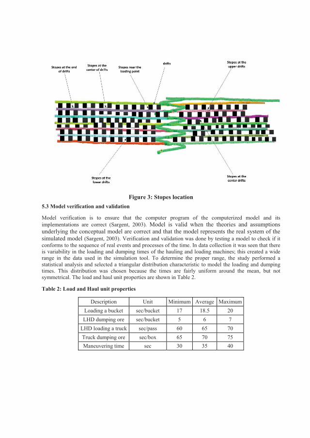
Figure 3: Stopes location5.3 Model verification and validation
Model verification is to ensure that the computer program of the computerized model and itsimplementations are correct (Sargent, 2003). Model is valid when the theories and assumptions underlying the conceptual model are correct and that the model represents the real system of the simulated model (Sargent, 2003). Verification and validation was done by testing a model to check if it conforms to the sequence of real events and processes of the time. In data collection it was seen that there is variability in the loading and dumping times of the hauling and loading machines; this created a wide range in the data used in the simulation tool. To determine the proper range, the study performed astatistical analysis and selected a triangular distribution characteristic to model the loading and dumping times. This distribution was chosen because the times are fairly uniform around the mean, but not symmetrical. The load and haul unit properties are shown in Table 2.
Table 2: Load and Haul unit properties
Description Unit Minimum Average MaximumLoading a bucket sec/bucket 17 18.5 20LHD dumping ore sec/bucket 5 6 7
LHD loading a truck sec/pass 60 65 70Truck dumping ore sec/box 65 70 75Maneuvering time sec 30 35 40

6. Simulation Results
Simulation was conducted independently for the stopes at the top, middle, and down drifts of the mine layout. For each simulated drift, the simulation was run at the end, centre, and near the loading point to determine the effect of reducing the tramming distance for the operation cycles. During simulation, the LHDs were fixed in the drifts, and the number of trucks was increased from 3 to 9. Figures 4, 5, and 6 compare production in these locations. Simulation results show that when 3 trucks and 3 LHDs are in operation at the top drifts, the amount of ore produced per month at the end, centre, and near the loading point is respectively 52 %, 53.7 %, and 54.8% of the planned production; for the mid-level stopes, production is 45.7 %, 49.8 %, and 51.6 % respectively, and for the lower levels, production is 42%, 44.4%, and 48.1% respectively.
The average production is greater when the LHDs are working near the loading point than when they are at the Centre or end of the drift. In all cases, the amount of ore produced increases as the number of trucks increases. With 4 and 5 trucks in operation, this means each LHD will serve one truck, and the extra trucks will be moving to the loading point of minimum queue. The increase in the number of trucks leadsto a reduction in individual truck utilization with lowest values noticed when operations are in the stopes which located at the end of the drift. The result is also indicating that, the increase in the number of trucks also increases LHD performance, especially when operations are at the end of the drift. It can be seen that the traffic is minimal when 3 trucks are in operation. The term traffic here refers to the percentage of the time lost when trucks meet in the haul ways. The traffic increases when the number of trucks starts to increase with the highest percent being noted when the LHDs are working near the loading point.
2 4 6 8 100
10
20
30
40
50
60
70
80
90
No. of Trucks
Pe
rce
nta
ge
(%
)
End of the drift
2 4 6 8 100
10
20
30
40
50
60
70
80
90Center of the drift
No. of Trucks
Pe
rce
nta
ge
(%
)
2 4 6 8 100
10
20
30
40
50
60
70
80
90Near the loading point
No. of Trucks
Pe
rce
nta
ge
(%
)
Ore producedTruck trafficTruck UtilizationLHD Utilization
Figure 4: Simulation results for the stopes located at the top drifts

2 4 6 8 100
10
20
30
40
50
60
70
80
90
No. of Trucks
Pe
rce
nta
ge
(%
)
End of the drift
2 4 6 8 100
10
20
30
40
50
60
70
80
90
100Near the loading point
No. of Trucks
Pe
rce
nta
ge
(%
)
2 4 6 8 100
10
20
30
40
50
60
70
80
90Center of the drift
No. of Trucks
Pe
rce
nta
ge
(%
)
Truck UtilizationOre producedTruck trafficLHD Utilization
Figure 5: Simulation results for the stopes located at the mid drifts
2 4 6 8 100
10
20
30
40
50
60
70
80
90
100
No. of Trucks
Pe
rce
nta
ge
(%
)
End of the drift
2 4 6 8 100
10
20
30
40
50
60
70
80
90
100Near the loading point
No. of Trucks
Pe
rce
nta
ge
(%
)
2 4 6 8 100
10
20
30
40
50
60
70
80
90
100Center of the drift
No. of Trucks
Pe
rce
nta
ge
(%
)
Truck trafficOre producedTruck UtilizationLHD Utilization
Figure 6: Simulation results for the stopes located at the lower drifts
7. Discussions
In all cases, the amount of ore produced increases when the number of trucks in operation increases. The production is greater when the mine is working on the stopes located in the upper drifts than those in the mid and lower drifts because trucks in the latter two cases have higher time to complete the cycle than the trucks in the former. When the number of trucks increases from 3 to 6, average production increases by 22%, 24%, and 26% for the upper, mid, and lower drifts respectively. The difference is not significantly greater due to the fact that trucks working on the upper drifts have a longer waiting time at the loading point than those on lower drifts. The truck waiting time increases when operations are going on at the far end of the drift; in this case, the LHDs spend more time loading and hauling material from the face to the loading point because of the longer tramming distance. When the stopes are backfilled and the length of the drift is decreased, the LHDs spend less time hauling and loading the trucks. Increasing the number of
trucks also leads to an increase in the LHDs performance and truck traffic. The traffic increases to 13% of the available time; which indicate that there is a time loss when trucks wait to give way to each otherwhen they meet at the intersection points on the ramp.
Production is sharply increased when the number of trucks is increased from 3 to 6. Beyond this point, the amount of ore produced does not rise at the same rate as the drop in truck utilization. It is observed that among all the simulated scenarios, a combination of 2 trucks and a single LHD for the upper drifts and 3 trucks and 1 LHD for the lower or mid drifts improves the average production to 75% of planned production. Reaching a production target of 100% proves infeasible in the given circumstances. Alternatively different haulage system should be considered, especially when the mine depth is increased
8. Conclusion
In an underground hard rock mine, the combination of LHDs and trucks play the important role in the rock material handling systems. The simulation technique was used to study their impact on the production. Three simulation models were created using SimMine software, to study the impact of these equipment for the productivity optimization. The results suggest that to improve the monthly production of ore, 1LHD can be assigned to serve a fleet of 2 trucks when working in the stopes close to the dumping point, and a fleet of 3 trucks can be used for the stopes on the mine’s lower levels. Future studies in this areashould consider using other type of low profile haul unit with bigger box size than the one used in this article, and also considering the increase of number of intersection points on the haul routes to reduce the truck traffic.
References
Banks, J, (1999). Descrete Event Simulation. Proceedings of the 1999 Winter Simulation Conference (ed: P.A. Farrington, H.B Nembhard, D.T. Sturrock, G.W Evans):7-13.
Banks, J, (2000). Introduction to simulation. Proceedings of the 2000 winter simulation conference, Orlando, 9-16.
B.Morgan (1994), Optimizing truck-loader matching. Proceedings of mine planning and equipment selection, 313-320
Greberg, J & Sundqvist, F (2011). Simulation as a tool for mine planning, in proceedings Second International Future Mining Conference, Melbourne, 273-278.
Saiang, D. (2008). Simulation of truck haulage queue system at an open pit mine using SIMIAN, Proceedings of the 5th International conference and exhibition on mass mining, 607-616.
Sabuncuoglu, I. & Hommertzheim, D.L, (1992). Dynamic dispatching algorithm for scheduling machines and automated guided vehicles in flexible manufacturing system. International journal of production research, 30, 1059-1079. doi: 10.1080/00207549208942943.
Sargent, R. G (2003). Verification and validation of simulation models. Proceedings of the 37th
Conference on winter simulation. 130-143. Syracuse, NY, USA.SimMine (Version 1.19) [Computer Software]. Malå, Sweden: SimMine AB.Stugul J.R & Li (1997). New development in simulation technology and applications in the mineral
industry, International Journal of Surface Mining, Reclamation and Environment, 11(4). 159-162.doi:10.1080/09208119708944087
Sweigard, R. (1992). Materials handling: Loading and haulage. In SME Mining Engineering Handbook, 2nd ed. Edited by H.L Hartman.Littleton, CO: SME.

PAPER B
The use of discrete event simulation for underground haulage mining equipment selection
Abubakary Salama, Jenny Greberg, and Håkan Schunnesson, The use of Discrete-Event Simulation for underground haulage mining equipment selection. Submitted for publication in the International Journal of Mining and Mineral Engineering


The use of discrete event simulation for underground haulage mining equipment selection
Abubakary Salama*, Jenny Greberg, and Håkan Schunnesson
Division of Mining and Geotechnical Engineering, Department of Civil, Mining and Environmental Engineering, Luleå University of Technology, SE-971 87 Luleå, Sweden
Abstract
The selection of equipment for haulage and transportation in underground mines is a challenge due to its impact on both production rates and costs. An under-dimensioned equipment fleet causes production losses, an over-dimensioned equipment fleet involves unnecessary additional capital costs as well as increased risk for traffic disturbances in the mine. Moreover, the combination of haulage and loading equipment needs to be optimized, the size of the different equipment types should create an optimal match for the complete system and also, the point in time when equipment is to be added or removed needs to be identified and well known before the change is made. Analytical methods are the traditional tools for equipment selection and these methods are still common, although the use of other tools such as discrete event simulation has been increasing during the last 10 years. In this paper, the use of discrete event simulation for equipment selection is discussed, and a case study where discrete event simulation was used to compare two different haulage units with the aim of improving production in an existing mine is presented. An overview of simulation of mining operations and an overview of analytical methods for equipment selection are also presented.
Keywords: Haulage system; equipment selection; discrete event simulation
*Corresponding author. Email: [email protected]

1. Introduction
The haulage system is one of the most important operations in underground mines as it is one of the main contributors to capital and operational costs. The haulage system involves the transportation of the mined out material from the primary phase to the secondary phase and then its further transportation to the mine surface (Atkinson, 1992). In the primary phase, the material is transported from the draw points to the loading areas where it is either stockpiledor further transported. In most underground hard rock mines, manual or automatic operated LHDs (Load-haul-dump) are used to load and transport the material due to their effectiveness in short distance transportation (Sweigard, 1992). The secondary phase involves the material being transported from the loading areas to the mine surface. In this phase, material can be transported both vertically and horizontally. Vertical transportation moves material vertically or near vertically and includes shafts, vertical conveyors, and hoisting systems. In horizontal transportation materials are moved horizontally through drifts and ramps with conveyors, rail or trucks. The choice of loading and hauling equipment will depend on various factors such as production requirements, dimensions of the haulage drifts, infrastructure layouts, material fragmentation, capital and operating cost, etc. Equipment selection has a significant effect on the efficiency and effectiveness of mining operations. The purchase of inappropriate vehicles for the mine fleets may result in an increase of the operational costs and lower the mine output. The haulage process that consists of loading activities, ore movement, and dumping operations involves uncertainty and random effects. Due to the existence of this uncertainty, simulation may be one among the most appropriate tools for equipment selection.
Discrete event simulation can be used to model systems which exhibit changes in state variables at a discrete set of points in time (Banks et al., 2010). The models can be static or dynamic. Static models represent a system at a specific time, while dynamic models represent a system as it evolves over a period of time (Law and Kelton, 1991). A mining operation is a dynamic system which is very difficult to model using analytical methods. When simulation is used, the model input can be based on probabilistic data which better characterize the input variables and a given number of variables can be described by selecting appropriate distributions. Examples of mining operations where simulation can be used are the flow of haul units in the mine and the flow of ore in the processing plant with the purpose of equipment optimization or ore blending.
This paper discusses the use of discrete event simulation for mine equipment selection, and illustrates the application of discrete event simulation for comparison of the production rates of two different types of hauling units. It focuses on material transportation by LHDs from draw points to loading bays, and trucks from loading bays to the bottom point of the shaft.
2. Equipment selection
In an underground mine, loading equipment is selected to match the size of the production, size of the openings, and number of faces in operations. Hauling equipment on the other hand is selected to meet the production requirements, and to be compatible with the loading equipment. In most cases, more emphasis is placed on selection of haulage equipment than on loading equipment (Ercelebi and Kirmanli, 2000). Some of the methods that are used for this selection are operations research methods, genetic algorithms, simulation, and analytical methods.

2.1 Loading equipment selection using analytical methods
Analytical methods have been widely used for many years in both open pit and underground operations. They evaluate load and haul combinations and factor in production constraints such as road conditions and rock characteristics (Atkinson, 1992) and (Ercelebi and Kirmanli, 2000). In sublevel open stoping, underground loaders extract ore from the stope and dump it directly into an ore pass or a loading bay or load it directly into the trucks that transport the ore further to the desired location. Several types of loaders are available including rail-mounted loaders, rubber-tired loaders, and shuttle loaders. Selection of the type of loader depends on the draw points, tipple access, loading bays, and stockpile bays. Draw points provide access to the stope for loading units to extract ore from the stopes. Tipple access allows loaders to easily tram and load without losing much time for turnaround or maneuvering. Stockpile bays keep the loaders producing while waiting for the trucks or full ore pass to clear. These bays need enough capacity to minimize delays to other parts of the production cycle. Rubber-tired loaders are effective in carrying load in the bucket for longer tramming distances. These types of loaders are commonly used in hard rock mines and are known as LHD machines, scoops, scoop trams, etc. An LHD may be diesel or electric powered. Diesel units are versatile and can easily move from one location to another. Electric units carry a cable drum and rely on trailing electric cable, they have low noise levels and zero emissions, and are highly productive in, for instance, block caving mines where ore is transported from a series of draw points to a fixed ore pass location (Sweigard, 1992).
The size of the selected LHD must fit into the planned development and stope openings, and also be able to reach a truck height and fill it efficiently. Its bucket capacity can be estimated based on the loader cycle time, bucket volume, broken density of the rock to be carried, and a fill factor which depends on rock fragmentation. The theoretical cycle time for the loader can be calculated by summing up the time to load and unload a bucket, travel time to and from the dumping point, and maneuvering time (Sweigard, 1992). The rock volume is converted into loose volume by the percentage of swell factor. The fill factor is a factor of the material sizing condition and how easy or difficult it is to fill the bucket and can be determined by field measurements (Atkinson, 1992). The maximum size of bucket is linearly correlated to the size of the machine. Based on the selected loading equipment, the type and number of hauling equipment is chosen to fit the loading units and to minimize delays in the operations.
2.2 Hauling equipment selection using analytical methods
Many different types of transportation equipment are available for material handling operations, including trucks, rails, conveyors etc. The selection of equipment should take into account the compatibility with the loading equipment. This study focuses on trucks, which today are used for the long haul of the material from the loading bays to the ore pass, shaft station, or directly to the mine surface. The selection of size and type of the trucks depends on various factors including, road geometry, production rate, haulage distance, mining method, ore reserve tonnage, haul road dimension, safety, capital and operating costs, road intersections, required truck speed, corners and bends, road quality, etc. For road geometry, itis important to take into consideration the turning radius at corners or in bends in order for the truck to be able to turn easily.
The size selection depends on the number of passes used by the loader to fill a truck. The combination of a truck with high capacity and a loader with low capacity will increase the number of loader passes required to fill the truck which leads to extended cycle time for the hauler and hence lower production. The optimal combination of loading and hauling units in operation can be obtained based on the Match Factor (Lizotte and Bonates, 1987). This

factor was first formulated by the Caterpillar Company to quantify the apparent balance which exists between the numbers of loading unit and haul unit. The factor is defined as shown in equation 1.
ctyl
ctyh
HNLN
MF**
(1)
In equation 1, MF stands for match factor, hN represents number of haul units, lN is the number of loading units, ctyL and ctyH are the load and haul cycle times respectively. When MF is below 1, it indicates that the system is under-trucked, while if it is above 1, it shows that the system is over-trucked. If it is exactly 1 it means that there is a theoretical match between haulers and loaders. The Match Factor calculations only provide an estimate of optimal balance between loader and trucks. The total number of vehicles, however, also depends on productivity estimate, available time in a shift, traffic disturbances etc. The theoretical truck cycle time excluding traffic disturbances, can be calculated with equation 2 (Atkinson, 1992). The cycle time depends on truck speed for different road grades, grade resistance and rolling resistance. If the road grades and resistances are higher the speeds of the haul units will be reduced, leading to increased cycle time.
ETLLTCT TDTLH (2)
In equation 2, CTH is the theoretical cycle time, TL is the loading time, LLT stands for haul travel time when the truck is fully loaded, TD represents dump time, and ET is the haul travel time when the truck is empty. When the cycle time is estimated, and the productivity per shift is known, the theoretical number of trucks can be estimated using equations 3, 4, and 5 (Atkinson, 1992).
CT
C
HEThrTonnes **60/ (3)
hrTonnesTN R
TRC /(4)
AVLUTL
TRC
TTNFleet
* (5)
Where CT is the truck capacity, TRCN stands for the theoretical number of trucks in operation, RT is the hourly required productivity, UTLT represents the truck utilization, AVLT is the mechanical availability of the truck, and E is the efficiency factor. Efficiency factor is used to estimate the truck productivity in the situation where the theoretical cycle time is used. Mechanical availability is an indication of the effectiveness of the maintenance programas well as the designed reliability, and can be calculated using equation 6 (Lyonnet, 1988).
HP
PAVL MO
OT (6)

In this equation, OP stands for operating hours and MH for maintenance hours. The estimated theoretical number of trucks does not include other factors such as queuing of trucks at loading and dumping points, traffic congestion etc. If queuing occurs, estimated queue length and queue time should be considered when estimating the fleet size. Traffic congestion occurs when the number of required trucks is high relative to the length of the haul. This can be minimized by effective traffic management through use of dispatching systems, well-spaced,efficient passing bays, etc. The loader can spend the time while the trucks are away to move the muck up material to a temporary stockpile at the loading point in order to minimize the loading time. Due to this, it is preferable to have loaders waiting for the trucks instead ofhaving the trucks waiting for the loader (Atkinson, 1992).
3. Equipment selection using simulation
Underground haulage operations involve uncertainty and random behavior. Neither uncertainty (for instance variances in mean time between failure, loading times, speed, and traffic) nor random behavior is considered when using analytical methods for equipment selection. In order to capture the effects of uncertainty and random behavior, the discreteevent simulation approach can be considered as one of the most appropriate techniques (Atkinson, 1992). The approach enables an estimation of the operational activities using probabilistic input data. Probabilistic data essentially represents a distribution of input data also providing a data range for different activities.
Simulation is defined as “the process of designing a model of a real system for the aim of understanding its behavior and to evaluate various strategies within the limits imposed by a criterion or set of criteria for the operation of the system’’ (Sturgul, 1999). The designed model usually takes the form of a set of assumptions for the operating system. These assumptions are expressed in mathematical, logical, and symbolic relationships between the objects of interest of the system (Banks and Carson, 1984). The models are analyzed by computational procedures and are ‘run’ to generate the results.
3.1 Discrete event simulation
The model of a system can be classified as discrete or continuous (Law and Kelton, 1991).Continuous systems are the ones where events occur continuously over a period of time. Examples are weather simulation, length measurement models, etc. In this study, discrete systems are considered. A discrete system is one where only a countable number of events can take place at any one instant in time (Sturgul, 1999). Discrete event simulation concerns the modeling of a system over time by representing the system changes as separate events. Aseparate event means that time progresses until the next event occurs. Monte Carlo techniques which involve the use of random numbers to simulate the actual statistical distributions that represent the entities of the system are utilized. Examples of discrete event systems that can be simulated are transportation systems, business processes, mining operations, emergency response systems, etc. Discrete event simulation also applies to different types of rules and procedures which increase the understanding of the interaction between variables and their importance in the system performance and provides suggestions on modificationsavailabilities in the system (Banks, 2000).
3.2 Discrete-event simulation in mining operations
Simulation in mining operations can be used to study various systems and various issues such as fleet requirements, flow of hauling machines and mine planning, with the aim of optimizing, improving, and planning the existing and future systems (Sturgul (1999).

Simulation can also be used by mining companies as a decision support tool and to increase the understanding of the mining system (Sturgul and Li, 1997). Simulation can handle complex mining systems which are discrete, change dynamically over a certain period of time and that are operated within a variable economic environment. Stochastic simulation of a mining system was first reported by Rist (1961). Since then several studies have shown a wide range of applicability of simulation studies in various operations in both underground and open pit mines (Raj et al, 2009). In South African mines, simulation has emerged as auseful means to explore the impacts of new capital investments and proposed mine methods(Turner, 1999). One example of a case study using simulation is the Ingwe Douglas Piller project where the simulation was conducted to determine the truck-shovel combinations suitable for a proposed mining operation. In Xu and Dong (1974) the application of discrete event simulation to develop a computer model of shovel and truck transportation system for an open pit mine in China was explained. The technique is widely used for both coal and hard rock mines for the analysis of haulage system. In Russia, computer simulation has been used for underground mining since the 1980s for developing the best correlations of the capacities of the haul units (Konyukh et al, 1999).
Sturgul (1999) was among the first to recognize the importance of simulation for use in mine planning and design. During the first symposium on the use of computers in mining, awork on computer simulation of a mine operation was published by Rist (1961), where a model was built to determine the optimum number of trains for a haulage level. Since then, the use of simulation has progressed to several mining aspects such as queuing theory, scheduling, decision making, location models, etc. One of the examples is truck-shovel simulation in a copper mine to simulate if a dispatcher could be used to route the trucks to different shovels to minimize queuing time and improve the operations (Sturgul, 1999).
In Europe, the first mine simulations appeared in 1950s to model the train transportation at the Kiirunavaara underground iron mine. The model was done by hand (Elbrond, 1964).Thereafter the development of the use of discrete simulation became more common in several countries. Mutagwaba and Durucan (1993) report an example from the United Kingdom where a simulation model for a mine transportation system was developed. Another exampleis the development of a simulation model to study the train transportation in underground coal mines in Germany (Wilke, 1970). Recently, the use of discrete event simulation has become popular in mining operations in Europe with studies in Sweden, Germany, Turkey (Panagiotou, 1999). In Australia, simulation has been used for various mining applications. An early project using computer simulation for developing ore handling operations at Mt. Newman Mining in Port Hedland, Western Australia was published in 1989 (Basu and Baafi, 1999). After that, several projects in both surface and underground mining in coal and hard rock have been carried out. Simulation modeling was used to optimize the underground ore handling at the Northparkes E26 Mine, and mine planning in the Newcrest Cadia East project (Greberg and Sundqvist, 2011).
In South America, there are several large copper, iron and bauxite mines in operation in various countries. Examples of these are the Chuquicamata, Teniente and Escondida operations in Chile, the Carajas mine of Brazil which operates the largest iron ore open pit in the world, and the Cerrejon coal mine which operates the largest truck fleet in the world(Knights and Bonates, 1999). The starting point for the use of discrete even mine simulation in South America is unclear as there is a lack of adequate scientific or engineering records.Knight and Bonates reported that several simulations models were developed in South America in the 1980s. One of the earliest papers relating to simulation modeling in South America is by Nogueira in 1984, which describes the application of a simulation model to improve truck-shovel operations at the CVRD Mine in Brazil. The model was designed to assess the best truck/shovel combinations in order to determine the capacity of the mine
operation. Another model was developed at Codelco Chile’s Teniente mine using GPSS/H (Sturgul, 1999). The model uses discrete simulation to simulate a system with continuous state variables. The t-test was performed to test the simulated results.
Generally, discrete simulation modeling has been used in mine planning and design, machine selection and the haulage system with the aim of optimizing the mine operations and production throughputs. Early studies focused mainly on limited parts of the mining process, such as for instance, equipment selection for the development stage, while more recent studies have aimed to cover more parts of the system and even to simulate a complete mine.
3.3 Simulation software
A large number of simulation languages are available and are widely used in mining operations for model formulation which means that the traditional methods such as manual calculations are less common when solving complex problems. The use of simulation tools increases the understanding of the system performance and the interaction of the variables involved. Simulation software can be divided into three categories (Banks et al, 2010). First, general purpose programming languages, such as Java, C, and C++ which offer a high degree of flexibility at a low cost, but require advanced programming skills (Sturgul and Jacobson, 1994). Second, simulation programming languages, such as SLAM, GPSS/H, SIMAN, ARENA, AUTOMOD, etc., which are object-oriented, discrete system simulation languageswith high flexibility and require some programming skills.
Third, mining specific software such as SimMine, which is a software that usesgraphical user interface with an environment that supports all aspects of a simulation. Due to the availability of a large number of simulation software solutions, careful selection should be made depending on the type of problem to be simulated. There are many issues to consider when selecting the software for the simulation studies. Some of these include; easy to use, availability of adequate debugging and error diagnostics, ability to import data from other software such as computer aided design and spreadsheet, availability of animation environment for easy visualization of the operations, quality of the output report and graphs for interpretation’’(Yuriy and Vayenas, 2008). In this paper SimMine software was selected for the analysis.
4. Example of the use of simulation for equipment selection
4.1 Mine operation description
The mine operation analyzed in this paper is a deep underground mine with an annual production of 2.62Mt pyrite and chalcopyrite. The mine has been in operation since 2000 and the mine is expected to be in operational until 2028. Ore is mined in three different zones A, B, and C with an average thickness of 3.5m, 3.1m, and 2.4m respectively. The mine uses four different mining methods. In zones A and B the ore is excavated with sublevel open stoping and Alimak mining. In zone C the ore is excavated with drift and fill mining and narrow vein mining. The focus in this study is on sublevel open stoping in zone A as shown in Figure 1.With this method, top and bottom accesses are mined from the ramp to reach the stope area. Slots between the top and bottom accesses are formed by conventional raises and occasionally drop raises. Stopes are drilled using both up holes from bottom access and down holes from the top access. Both up holes and down holes are 10 m long and reach to half the distance between the two drives. When a stope is mined and mucked out, the opening is backfilled with paste.
The mine uses paste fill which consists of a mixture of granite aggregate, tails, and 2.5% or 6.5% cement content. The 2.5% recipe are used to backfill stopes in the area where mining

operations will not continue to the level above, while the 6.5% recipe is used when the miningoperations will take place on the level above the stope. The required strength is 90kPa for the 2.5% recipe and 350kPa for the 6.5%. In order to minimize dilution, mining of adjacent stopes can start only when the required strength is achieved. In the mining area considered in this paper (zone A), the major production occurs at mine drifts below the lowest point of the main shaft. Here, the lowest level of production is about 300m vertical distance from the shaft’s lowest loading point. Below these levels, mine development is in progress.
Figure 1. Schematic layout for sub level open stoping method
4.2 Current haulage system
Immediately after the blast, when the stope is not supported, the mine utilizes automaticallyoperated LHDs to load the ore from the stope to the loading bay. After the stope has been supported, conventional LHDs are used to load the ore from the stope to a loading bay. From the loading bay TH430 trucks are used to haul the ore to the shaft loading point, from where the ore is hoisted to the surface, see Figure 2. Currently three LHDs are assigned to operate, in three different stopes, and three trucks haul the ore from each stope to the shaft. Currently,this equipment fleet only produces 52% of the planned production. It is assumed that the reasons for the low production are limited size of drifts, the ramp design, and traffic interference in the ramps, etc. All these factors increase the cycle time of the trucks, reducing overall equipment effectiveness and mine output.
In this study, the haulage system is simulated in order to optimize the number of trucks for the studied mine production system, to increase the mine output and to evaluate the possibilities to reach the assigned production targets. Furthermore, in order to optimize production a productivity comparison is also made between two different types of trucks. Truck type one is a TH430 which has a theoretical capacity of 25-30 tonne. Truck type two is a TH660 with a payload of 50-55 tonne.

Figure 2. Flow chart for haulage system of this mine
4.3 Simulation Data input
4.3.1 Shift schedules
The mine operates two shifts per day of 10 hours each. The dayshift starts at 6:00 a.m. and ends at 4:00 p.m., with two hours assigned for meal break and shift preparations. The nightshift starts at 6:00 p.m. and ends at 4:00 a.m., also with two hours for shift preparations and meal break. Blasting is conducted once a day during the shift change.
4.3.2 Machine description
The properties of the loading and hauling machines are based on information collected in the mine. The parameters include: the speed of empty and fully loaded vehicles at flat, incliningand declining roads, tire rolling resistance and ramp gradient, as shown in Table 1.
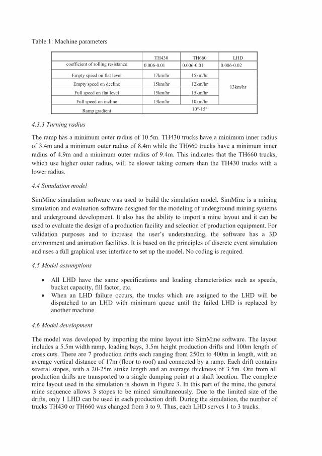
Table 1: Machine parameters
TH430 TH660 LHD coefficient of rolling resistance 0.006-0.01 0.006-0.01 0.006-0.02
Empty speed on flat level 17km/hr 15km/hr
13km/hrEmpty speed on decline 15km/hr 12km/hr
Full speed on flat level 15km/hr 15km/hr
Full speed on incline 13km/hr 10km/hr
Ramp gradient 10°-15°
4.3.3 Turning radius
The ramp has a minimum outer radius of 10.5m. TH430 trucks have a minimum inner radius of 3.4m and a minimum outer radius of 8.4m while the TH660 trucks have a minimum inner radius of 4.9m and a minimum outer radius of 9.4m. This indicates that the TH660 trucks, which use higher outer radius, will be slower taking corners than the TH430 trucks with alower radius.
4.4 Simulation model
SimMine simulation software was used to build the simulation model. SimMine is a mining simulation and evaluation software designed for the modeling of underground mining systems and underground development. It also has the ability to import a mine layout and it can be used to evaluate the design of a production facility and selection of production equipment. For validation purposes and to increase the user’s understanding, the software has a 3D environment and animation facilities. It is based on the principles of discrete event simulation and uses a full graphical user interface to set up the model. No coding is required.
4.5 Model assumptions
All LHD have the same specifications and loading characteristics such as speeds, bucket capacity, fill factor, etc.When an LHD failure occurs, the trucks which are assigned to the LHD will be dispatched to an LHD with minimum queue until the failed LHD is replaced by another machine.
4.6 Model development
The model was developed by importing the mine layout into SimMine software. The layout includes a 5.5m width ramp, loading bays, 3.5m height production drifts and 100m length of cross cuts. There are 7 production drifts each ranging from 250m to 400m in length, with an average vertical distance of 17m (floor to roof) and connected by a ramp. Each drift contains several stopes, with a 20-25m strike length and an average thickness of 3.5m. Ore from all production drifts are transported to a single dumping point at a shaft location. The complete mine layout used in the simulation is shown in Figure 3. In this part of the mine, the general mine sequence allows 3 stopes to be mined simultaneously. Due to the limited size of the drifts, only 1 LHD can be used in each production drift. During the simulation, the number of trucks TH430 or TH660 was changed from 3 to 9. Thus, each LHD serves 1 to 3 trucks.

Figure 3. Mine layout of zone A area.
The LHD tramming distance depends on the length of the production drift. The tramming distance is defined as the distance from the active face to the loading bay. The cycle time will be longer for equipment working at the far end of the drift than for equipment in the middle or near the loading bay. Therefore, the simulation was run separately for the stopes located at the end, center, and near the loading point of the drift. The total length of the haul road includes 800m ramp, 800m main level, and 100m cross cuts. To reach the dumping points, a truck from the lower levels travels from loading points through cross cuts, ramp and main level, while those from the upper drifts also travel a small portion of the ramp before entering the main level. To check for the effect of haulage distance to the dumping point, the simulation was repeated by changing the stope locations. Figure 4 shows the stopes selected from the top drifts in the first run, the middle drifts in the second, and the bottom drifts in the third. As shown in Figure 4, stopes located from drifts 1 to 3 are termed as upper drift stopes, those in drifts 3 to 5 are classified as mid-drift stopes, and those in drifts 5 to 7 are called lower drift stopes. The simulation was run for three stopes at a time; two stopes were chosen from the same drift but on opposite sides, and the third was taken from the two drifts down or up for stability reasons. For example, for the upper drift stopes, if two stopes are chosen from drift 1, the third will be chosen from drift 3.
Figure 4. Mine stopes location

4.7 Model verification and validation
The model is verified in order to ensure that the computerized model and its implementations are correct (Sargent, 2003). A model is valid when the theories and assumptions underlying the conceptual model are correct and the model represents the real system (Sargent, 2003).Verification and validation was done by testing the model to check if it conforms to the sequence of real events. During the data collection variability in the loading and dumping times of the hauling and loading machines was seen. To determine the proper range of input data, a statistical analysis was performed and a triangular distribution characteristic was selected to model the loading and dumping times. This distribution was chosen since the times are fairly uniform around the mean, but not symmetrical. The load and haul unit properties are shown in Table 2. As can be seen, the loading time per pass differs for the two truck types because of both the loading capacity and the height of the truck boxes. TH430 has a box height of 2.3m and a capacity of 30 tonnes, while truck TH660 has a box height of 3.4m and a capacity of 60 tonnes. Therefore the loading unit spends more passes and lifting time to fill truck TH660 than truck TH430.
Table 2. Load and dump times for TH430 and TH660
Description Unit Minimum Average Maximum
LHD loading TH430 sec/pass 60 65 70
LHD loading TH660 sec/pass 72 76 80
TH430 dumping ore sec/box 65 70 75
TH660 dumping ore sec 65 70 75
TH430 Maneuvering time sec 30 35 40
TH660 Maneuvering time sec 70 82.5 95
5. Simulation results
The simulation was first conducted for the stopes located at the upper drifts in order to compare with the real mine case. Currently the mine operates with 3 LHDs and three TH430trucks (one assigned to each LHD). In relation to schedule production based on the design and the overall mine plan, the set up with three LHDs and three TH430 trucks only produces 52% of the planned production. Figure 5 shows the productivity comparison between the TH430trucks and the TH660 trucks for the upper drifts. When considering TH430 for three trucks served with three LHDs, the amount of ore produced is 53% which indicates that the simulated result is close to the real operation in the mine. In comparison with both truck types, the amount of ore produced at the end, center, and near the loading bay seems to be slightly higher for the TH660 than that of TH430 even though the pay load for the TH660 is twice as high as for the TH430. In all cases, the amount of ore produced increases as the number of trucks increases. With 4 and 5 trucks in operation each LHD will serve one predetermined truck, while the extra trucks will be directed from dispatch to move to the LHD that has no queue. The average ore produced for both truck types for mid and lower drifts was observed to be lower than that of the top drifts as shown in Table 3.

Figure 5. Percentage of ore produced for the TH430 and TH660 trucksAs can be seen in Figure 6, the increased number of trucks leads to a reduction in truck
utilization for both truck types with the lowest utilization values noticed when operations are in the stopes located at the end of the drift. It shows that TH430 trucks have higher utilizations compared to the TH660 trucks. The average truck utilizations for top drifts at the end, center, and near the loading point for both truck types are lower compared to when these trucks operated at mid and lower drifts as shown in Table 3.
It also shows that an increased number of trucks lead to increased LHD utilization as shown in Figure 7. In this figure, it can also be seen that the LHDs which are serving TH660 trucks have higher utilization than for TH430 trucks. One reason for this may relate to the number of passes needed to load a truck. On average 3 passes are used to load a TH430 truck while 5 passes are used for a TH660 truck. The average LHD utilization for top drifts at the end, center, and near the loading point for both truck types are higher compared to LHDs operated at mid and lower drifts as shown in Table 3.
Figure 6. Utilization of the trucks

Figure 7. LHDs Utilizations
The term traffic refers to the percentage of time lost when trucks meet in the haul ways (the main drift and the ramp). It can be seen in Figure 8 that the traffic is minimal when three trucks are in operation, but the traffic increases when the number of trucks starts to increase. Due to the long box size of TH660 trucks, a great deal of time is consumed when they meeteach other, which generates higher traffic than for the TH430 trucks. As seen in Figure 8, the highest percentage of traffic is when the LHDs are working near the loading point, due to the short waiting times for the trucks at the loading point and thus longer time spent for transportation on the main level where other trucks are present. On average, the traffic for upper drifts was observed to be lower than for the mid and lower drifts as shown in Table 3.
Figure 8. Traffic comparisons of the trucks
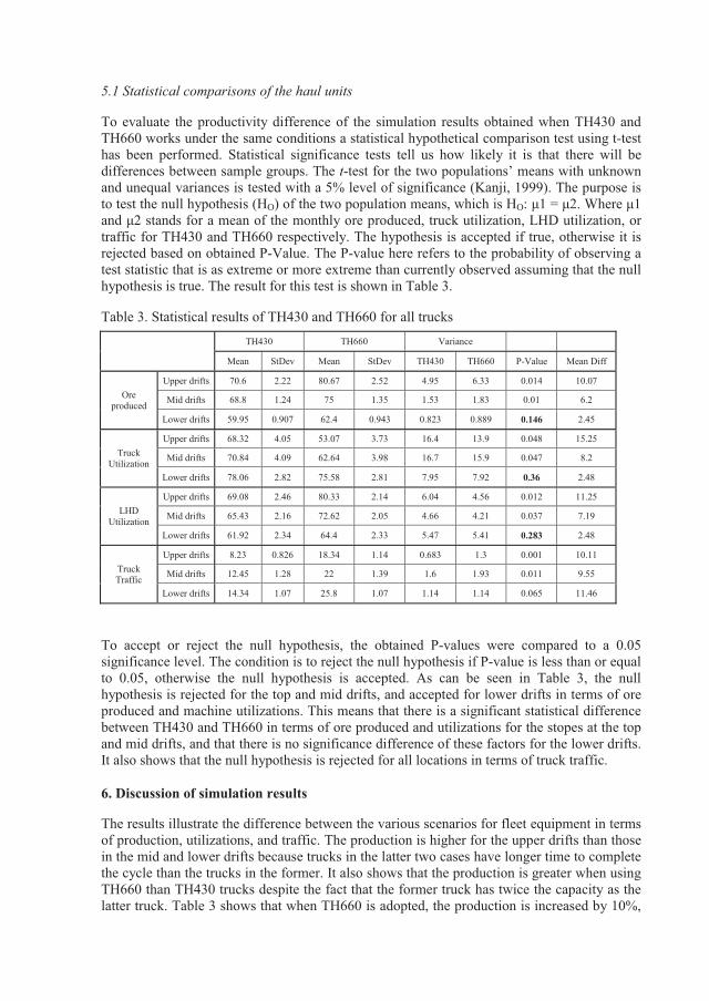
5.1 Statistical comparisons of the haul units
To evaluate the productivity difference of the simulation results obtained when TH430 and TH660 works under the same conditions a statistical hypothetical comparison test using t-test has been performed. Statistical significance tests tell us how likely it is that there will be differences between sample groups. The t-test for the two populations’ means with unknown and unequal variances is tested with a 5% level of significance (Kanji, 1999). The purpose is to test the null hypothesis (HO) of the two population means, which is HO:
traffic for TH430 and TH660 respectively. The hypothesis is accepted if true, otherwise it isrejected based on obtained P-Value. The P-value here refers to the probability of observing a test statistic that is as extreme or more extreme than currently observed assuming that the null hypothesis is true. The result for this test is shown in Table 3.
Table 3. Statistical results of TH430 and TH660 for all trucksTH430 TH660 Variance
Mean StDev Mean StDev TH430 TH660 P-Value Mean Diff
Ore produced
Upper drifts 70.6 2.22 80.67 2.52 4.95 6.33 0.014 10.07
Mid drifts 68.8 1.24 75 1.35 1.53 1.83 0.01 6.2
Lower drifts 59.95 0.907 62.4 0.943 0.823 0.889 0.146 2.45
Truck Utilization
Upper drifts 68.32 4.05 53.07 3.73 16.4 13.9 0.048 15.25
Mid drifts 70.84 4.09 62.64 3.98 16.7 15.9 0.047 8.2
Lower drifts 78.06 2.82 75.58 2.81 7.95 7.92 0.36 2.48
LHD Utilization
Upper drifts 69.08 2.46 80.33 2.14 6.04 4.56 0.012 11.25
Mid drifts 65.43 2.16 72.62 2.05 4.66 4.21 0.037 7.19
Lower drifts 61.92 2.34 64.4 2.33 5.47 5.41 0.283 2.48
Truck Traffic
Upper drifts 8.23 0.826 18.34 1.14 0.683 1.3 0.001 10.11
Mid drifts 12.45 1.28 22 1.39 1.6 1.93 0.011 9.55
Lower drifts 14.34 1.07 25.8 1.07 1.14 1.14 0.065 11.46
To accept or reject the null hypothesis, the obtained P-values were compared to a 0.05 significance level. The condition is to reject the null hypothesis if P-value is less than or equal to 0.05, otherwise the null hypothesis is accepted. As can be seen in Table 3, the null hypothesis is rejected for the top and mid drifts, and accepted for lower drifts in terms of ore produced and machine utilizations. This means that there is a significant statistical difference between TH430 and TH660 in terms of ore produced and utilizations for the stopes at the top and mid drifts, and that there is no significance difference of these factors for the lower drifts. It also shows that the null hypothesis is rejected for all locations in terms of truck traffic.
6. Discussion of simulation results
The results illustrate the difference between the various scenarios for fleet equipment in terms of production, utilizations, and traffic. The production is higher for the upper drifts than those in the mid and lower drifts because trucks in the latter two cases have longer time to complete the cycle than the trucks in the former. It also shows that the production is greater when using TH660 than TH430 trucks despite the fact that the former truck has twice the capacity as the latter truck. Table 3 shows that when TH660 is adopted, the production is increased by 10%,

6%, and 3% at upper, mid, and lower drifts respectively. In this mine area, only three stopes can be extracted at a time due to safety, the size of the hoisting shaft, and the waiting time for paste fill to reach the required strength. Therefore there is no possibility to increase the number of active stopes to increase production. This indicates that as mine depth increases,the use of bigger haul units is not a main factor for production improvement as the costs associated in changing truck size might not be recuperated by extra production.
It is anticipated that production should be much higher in upper levels compared to the lower levels due to the fact that trucks traveling on the upper drift have less cycle time than the ones in the lower levels. But as seen, the difference is not higher due to the reason that these trucks have a longer waiting time at a loading point and they also travel a small portion of the ramp to reach the dumping point which increases their time loss. The truck waiting time increases when operations are going on at the far end of the drift. In this case, the LHDs spend more time loading and hauling material from the face to the loading point because of the longer tramming distance. Normally, automatic LHDs are used to muck the material immediately after the stope is blasted and dumped at the stockpile located at the loading pointof each production drift. During this operation, the manual LHDs and haul trucks are not working due to the unsafe condition of the stope. After the stope has been stabilized, the normal loading equipment will start mucking the stope and load to the trucks. When there is no truck waiting at the loading point, the LHDs will also dump the material at the stockpile.
As shown in Figure 5 for both truck types, production is increased when the number of trucks is increased from three to six. Beyond this point in the Figure, the amount of ore produced does not rise at the same rate. Instead a drop in truck utilization can be noted. The truck utilization is observed to be higher when TH430 is used. This is because TH430 has higher speed than TH660 in the same working conditions. Increasing the number of trucks also leads to an increase in the LHD utilization. LHDs which are serving TH660 have higher utilization because of the larger number of passes needed to load this trucks. Also more time is consumed to stockpile material before these trucks arrive for the next load.
As depicted in Table 3, there is no significance difference for the upper, mid, and lower drifts when considering truck traffic. The traffic increases from 8% to 14% when TH430 is used and from 18% to 26% when using TH660. This indicates that TH660 trucks have ahigher time loss when waiting to give way to each other, when they meet at the intersection points between ramp and crosscuts, and when they meet at the corner points. This indicatesthat the ramp will be one of the main causes of production delay when more production drifts are in operation for deeper levels.
It is observed that among all the simulated scenarios, a combination of 2 trucks and a single LHD for the upper drifts and 3 trucks and 1 LHD for the lower or mid drifts improves the average production from 52% to 75% of planned production when TH430 is used, and to 83% when TH660 is used. Reaching a production target of 100% proves infeasible under the given circumstances. The possible alternative to the production improvement could be addition of another ramp to minimize truck traffic, extension of the existing shaft or adding another shaft to reduce haul distance to the existing shaft point, or considering a different haulage method especially when the mine depth is increased.
6.1 Discussions on the use of discrete event simulation
Underground haulage fleet selection involves the choice of equipment suitable for transportation of materials from extraction faces to the shaft portals or mine surface. The process consists of many uncertainties and random behavior operations such as variation of ramp grade, haulways, variable vehicle speeds, and equipment payloads. The existence of many uncertain operational elements and the random behavior of the system makes fleet

selection less accurate using analytical calculation since the calculation does not explicitly acknowledge the uncertainty and randomness. The most useful methods for the fleet selection considering uncertainty and randomness are simulation and mathematical programming (Elbrond and Soumis, 1987). Discrete event simulation approach was considered as the most appropriate technique to deal with such operations as it is known for having the advantage of more accurate accounting for the real world uncertainty and diversity to the variability of the interdependent components within the operations.
Discrete event simulation has an ability to model complex systems in great detail and to provide more accurate results. A verified and validated simulation model could provide results that are very close to those seen in the actual operating system. This high accuracy comes at the expense of high modeling and computational effort. Developing a detailed, more accurate simulation model for a large and complex system requires the collection of a large amount of data, the fitting of that data to statistical distributions and a careful choice of simulation software. The probabilistic nature of many events such as ramp grade variation, haul truck speeds, and machine failures can be represented by sampling from the probabilisticdistribution behavior of the data representing a pattern of the occurrence of the event. Thus, to represent a typical behavior of the system, and obtain the performance measure estimates with high confidence levels, it is necessary to run the simulation model many times so that many events can occur a large number of times. To increase efficiency, discrete event simulation can be equipped and combined with economic analysis models to improve understanding of the behavior of various systems, and reduce risk when selecting the operational systems.
7. Conclusion
The application of discrete event simulation for comparison of the production rate of two different types of hauling units has been discussed. The various scenarios for fleet equipment in terms of production, utilization and traffic were simulated. The results show that, among all the simulated scenarios, a combination of 2 trucks and a single LHD for the upper drifts and 3trucks and 1 LHD for the lower or mid drifts improves the average production from 52% to 75% of planned production when the TH430 is used, and 52% to 83% when the TH660 is used. These indicate that there is no high impact on production improvement when TH430 is replaced by TH660 as production will rise only by 8%. This may need to be justified financially as the costs associated with changing the truck size might not be recuperated byextra production. Reaching a production target of 100% seems to be infeasible under the given circumstances. It is suggested that the possible alternative for production improvement could be the addition of another ramp to minimize truck traffic, extension of the existing shaft or adding another shaft to reduce haul distance to the existing shaft point, changing the mine plan and scheduling, or considering a different haulage method especially when the mine depth is increased.
Acknowledgements
The authors would like to thank the I2Mine project within the EU 7th framework programme for funding parts of the work and its great help towards the completion of this work.

References
Atkinson, T. (1992) ‘Selection and sizing of excavating equipment’, in SME Mining Engineering Handbook’, H.L Hartman, 2nd ed., Littleton CO SME, pp1311-1333
Basu, A. J and Baafi E.Y. (1999) ‘Discrete event simulation of mining systems, Current practice in Australia’, International Journal of Mining, Reclamation and Environment,Vol. 13 No. 2, pp. 79-84.
Banks, J. (1999) ‘Discrete event simulation’, Proceedings of the 1999 Winter Simulation (eds: P.A. Farrington, H.B Nembhard, D.T. Sturrock, G.W Evans), Phoenix, AZ, USA, pp.7-13.
Banks, J., Carson, J.S, Nelson, B.L and Nicol, D.M. (2010) ‘Discrete event System simulation’, Pearson Education, New Jersey.
Banks, J. and Carson II, J.S. (1984) ‘Discrete-event system simulation’, Prentice Hall, Englewood Cliffs, New Jersey.
Banks, J. (2000) ‘Introduction to simulation’, Proceedings of the winter simulation, Orlando, 2000, pp. 9-16
Morgan, B. (1994) ‘Optimizing truck-loader matching’, Proceedings of mine planning and equipment selection, Istanbul, pp 313-320.
Caterpillar (2001) ‘A reference guide to Mine Machine Applications’, Peoria, IL, Caterpillar.Elbrond, J. (1964) ‘Capacity calculations at LKAB, Kiruna’, in APCOM 1964. Proceedings
Denver CO. (Published. by Colorado School of mines), pp. 683-690.Elbrond, J. and Soumis, F. (1987) ‘Towards integrated production planning and truck
dispatching in open pit mines’ International Journal of Mining, Reclamation and Environment, Vol. 1, pp. 1-6.
Ercelebi, S.G and Kirmanli, C. (2000) ‘Review of surface mining equipment selection techniques’, Mine Planning and Equipment Selection, Ed Pasamehmetoglu. Et al. Balkema, Rotterdam, pp 547-553.
Panagiotou, G.N. (1999) ‘Discrete mine system simulation in Europe’, International Journal of Mining, Reclamation and Environment, Vol. 13 No. 2, pp. 43-46
Raj, M.G. Vardhan, H. and Rao, Y.V (2009) ‘Production optimization using simulation models in mines: a critical review’, International Journal of Operational Research, Vol. 6 No. 3, pp. 330-359
Greberg, J. and Sundqvist, F. (2011) ‘Simulation as a tool for mine planning’, in Proceedings of Second International Future Mining, Melbourne, pp. 273-278
Yuriy, G. and Vayenas, N. (2008) ‘Discrete-event simulation of mine equipment systems combined with a reliability assessment model based on genetic algorithms’, International Journal of Mining, Reclamation and Environment, Vol. 22 No. 1, pp. 70-83
Sturgul, J.R (1999) ‘Discrete mine system simulation in the United states’, International Journal of Mining, Reclamation and Environment Vol. 13 No. 2, pp. 37-41.
Kanji, G. (1999) ‘100 statistical tests’, Sage: Thousand Oaks, CA, pp. 23-30.Lyonnet, P. (1988) ‘Maintenance planning methods and mathematics’, Chapman & Hall.Mutagwaba, W. and Durucan, S. (1993) ‘Objecte-oriented simulation in mine transportation
design’, Proceeding of Mine Mechanization and Automation, G.Almgren, U. Kumar and N. Vagenas (eds), Rotterdam:Balkema, pp. 591-600
Nogueira, J.A. (1984) ‘Controle de Equipamentos e Dispatching. Seminario O Computador e -96

Knights, P.F. and Bonates, E. J.L. (1999) ‘Applications of discrete mine simulation modeling in South America’, International Journal of Mining, Reclamation and Environment,Vol. 13 No. 2, pp. 69-72
Rist, K. (1961) ‘The solution of a transport problem by use of Monte Carlo Technique’, Paper presented at the APCOM 1, Arizona, USA.
Turner, R.J (1999) ‘Simulation in the mining industry of South Africa’, International Journal of Mining, Reclamation and Environment, Vol. 13 No. 2, pp. 47-56
Sabuncuoglu, I. and Hommertzheim, D.L. (1992) ‘Dynamic dispatching algorithm for scheduling machines and automated guided vehicles in flexible manufacturing system’,International Journal of Production Research, Vol. 30, pp. 1059-1079
Sargent, R.G. (2003) ‘Verification and validation of simulation models’, Proceedings of the 37th Conference on winter simulation, Syracuse, NY, USA, pp. 130-143
Sturgul J.R and Jacobson, W.L. (1994) ‘A simulation model for testing a proposed mining operation’, Phase 1. Mine Planning and Equipment Selection, Pasamehmetoglu et al. ed (Rotterdam: Balkema), pp. 281-287
Sturgul J.R and Li, (1997) ‘New development in simulation technology and applications in the mineral industry’, International Journal of Mining, Reclamation and Environment,Vol. 11 No. 4, pp. 159-162
Sweigard, R. (1992) ‘Materials handling: Loading and haulage’, In SME Mining Engineering Handbook, 2nd ed. Edited by H.L Hartman.Littleton, CO: SME.
Konyukh, V., Galiyev, S. and Li, Z. (1999) ‘Mine simulation in Asia’, International Journal of Mining, Reclamation and Environment, Vol. 13 No. 2, pp. 57-67
Wilke, F.L (1970) ‘Simulation studies of computer controlled traffic underground in large coal mines’, 9th International Symposium on Decision Making in the Mineral Industry,Can 1MM, sp. Vol. 12, pp. 344-351.
Xu, G. and Dong, Z. (1974) ‘Mathematical simulation of the mining process at Mines’, Practice and Knowledge of mathematics, Vol. 4, pp. 26-37 (in Chinese).
Lizotte, Y. and Bonates, E. (1987) ‘Truck and shovel dispatching rules assessment using simulation’, International Journal of Mining, Reclamation and Environment, Vol. 5, pp. 45-58
Law, A.M and Kelton, W.D (1991) ‘Simulation Modeling analysis’, Second edition, McGraw-Hill, New York.

PAPER C
Operating Value Optimization using Simulation and Mixed Integer Programming
Abubakary Salama, Micah Nehring, Jenny Greberg, Operating Value optimization using Simulation and Mixed Integer Programming. Accepted for publication in the International Journal of Mining, Reclamation and Environment

Operating Value Optimization using Simulation and Mixed Integer Programming
Abubakary Salama1*, Micah Nehring2, Jenny Greberg1
1Division of Mining and Geotechnical Engineering, Department of Civil, Mining and Environmental Engineering, Luleå University of Technology, SE-971 87 Luleå, Sweden;2School of Mechanical and Mining Engineering, The University of Queensland, St Lucia,
QLD, Australia, 4072
Abstract
Mining operations around the world will increasingly need to operate at greater depths. This significantly influences the complexity of ore extraction and ore transportation to the surface. The increase in mine depth leads to increases in haulage distance from mine areas to the mine surface. This results in an increase in energy costs to haul material further. Due to the increasing cost of future operations, the choice of the haulage method becomes an important factor in the optimization of the mine plan. The haulage process is one of the most energy intensive activities in a mining operation, and thus, one of the main contributors to energy cost. This paper presents the comparison of the operating values of the mine plans at depth levels of 1,000, 2,000, and 3,000 meters for diesel and electric trucks, shaft and belt conveyor haulage systems for the current and a predicted future energy price scenario. The aim is to analyze the impact of energy requirements associated with each haulage method, as well asthe use of alternative sequencing techniques as mine depth increases. This study is carried out using a combination of discrete event simulation and mixed integer programming as a tool to improve decision making in the process of generating and optimizing the mine plans. Results show that energy cost increases across each haulage method at both current and future energy prices, with increasing depth. This study thus provides a broad and up to date analysis of the impact on operating values that may be experienced with the use of the main haulage systems available at present. Also, the study shows how the combination of discrete event simulation and mixed integer programming generates a good tool for decision support.
Keywords: Discrete event simulation, Mixed Integer Programming, Deep Mining, Haulage Energy
*Corresponding author. Email: [email protected]

1. IntroductionAs mining companies rapidly exploit the near surface deposits, the mining frontiers of the future will be deeper, more remote, and more hostile. In addition, mining operations will facemore extreme climatic conditions, and they will occur in unstable ground, with less water and less energy availability. While these conditions present huge challenges in themselves, all this will be against a backdrop of more intensive public scrutiny over environmental issues and community relations. Whether true or not, politicians will increasingly use public perceptions in policy making decisions which in Australia has recently resulted in the introduction of sweeping new taxes on coal and iron ore producers through the Mineral Resources Rent Tax (MRRT) as well as the introduction of a broader carbon tax in the name of environmental protectionism.
More so now than ever, mining companies must be able to investigate the implications of the increased cost of energy, water and other resources on their mine plan, and be able to adapt. One important aspect in being able to adapt is to firstly know what options are available and how a mine plan may be impacted through their implementation. With this inmind, this paper presents a case study of an underground ore body amenable to sublevel stoping. An analysis takes place which compares operating values of the mine plans generated for the ore-body at depth levels of 1,000 m, 2,000 m and 3,000 m, using diesel and electric trucks operating in shafts and conveyors as haulage systems at current, and three times the current energy prices, using discrete event simulation combined with mixed integer programming.
This paper thus investigates and discusses, from an operating value and mine planning perspective, the implications of mining in an environment of increasing energy costs, increased environmental scrutiny and the requirement to perform larger scale mining activity at increasing depths. There is no doubt that this is the reality facing the mining industry worldwide, and it would appear that much of the mining academic and research community has also shifted its focus in a large way to reflect this reality. At a recent research retreat, the division of Mining Engineering at The University of Queensland decided to form the Centre for Deep Mining for the purpose of focusing its broad research activities on a central key theme. Another example of this has been the launch of the I2 Mine (Innovative Technologies and Concepts for the Intelligent Deep Mine of the Future) project by the European Commission involving a consortium of 26 industry and research organizations from 10 European countries. This project is stated by the funders as ‘marking the start of a series of activities designed to realize the concept of an invisible, zero-impact mine’ and ’will concentrate on the development of technologies suitable for deep mining activities’ [14]. The division of Mining and Geotechnical Engineering at Luleå University of Technology, Sweden is part of this research project which is one of the numerous projects aimed at improving mining operations at great depth. This paper presents the results of a study carried out to realize the stated objective.
2. Haulage systems
The haulage system is one of the most intensive users of energy in a mining operation and is thus one of the main contributors to the total energy cost. As the number of underground mines operating at greater depth increases, the haulage method is among one of the most important factors in optimizing mine production. Therefore, hauling ore from deeper levels needs to be evaluated in order to account for energy costs associated with hauling options. In this paper, four haulage systems are analyzed using Discrete Event Simulation and Mixed Integer Programming to aid the mine planning process.

2.1. Truck haulage
Truck haulage systems are widely used in underground operations for material transport from draw points to storage bays and crushers, or to the mine surface. With an increase in mine depth, haul distance from the draw points to the mine surface increases, this leads to an increase in the operating costs of trucks [1]. Diesel powered equipment has become increasingly utilized in mining since their introduction into operations in the 1960s with significant subsequent efforts to improve productivity and safety. The main advantages associated with the use of diesel equipment include; flexibility in travel routes, flexibility in the size of the fleet, absence of electrical hazards, high productivity, rapid haulage speed, generally good reliability and low operating cost [3]. Disadvantages of these vehicles are the use of flammable fuel, higher capital cost, higher heat emission, higher noise level and emission of toxic gases and particulates [4]. This study uses diesel and electric trucks to compare energy consumption at various mine depths. Both types of trucks were simulated based on similar working conditions. Loading and hauling properties are described based on information from the manufacturer and data from mine site. Both truck types are loaded at the storage bin located beneath the crusher station. During loading and dumping, electric trucks leave the trolley line and use a diesel driven motor.
2.1.1. Energy consumption by dump trucks
Energy consumption of dump trucks depends on the hauling distance from the loading point to the dumping point, payload, speed of the vehicle, mine topography, engine capacity andload factors, etc. When a truck moves, the engine generates power against friction, air, rolling and gradient resistance. The energy consumption of the diesel truck was estimated using equation 1[1].
= (1)
Where LMPH is the liters used per machine hour, K stands for the kilogram of fuel used per brake horsepower per hour, GHP represents the gross engine horsepower at governed engine revolution per minute, KPL is the weight of fuel in Kg/liter, and LF is the load factor in percentage. The load factor is defined as the portion of full power required by the truck. According to [13], the engine load factors are termed as Low: 20%-30%, low load factor, excellent haul road condition, no overloading, Medium: 30%-40%, moderate road factor, good haul road condition, minimal overloading, High: 40%-50%, high load factor, poor haul road condition, overloading. The energy consumption of the electric truck depends on the engine size, operator efficiency, condition of the equipment, and was estimated based on aload factor, condition of the equipment, and gross engine horsepower. In modeling, engine load factors of 35% for empty, 50% for full diesel and electric trucks, and diesel oil density of 0.85kg/l [2] were used.
2.2. Shaft haulage
Shaft is one of the most important openings of an underground mine which is sunk into the earth to access mineral resources which are too deep to mine economically using open cut methods. Shafts are also used to provide various services such as ventilation, power and water supply. The design of the mine shaft requires the consideration of several variables to ultimately arrive at economic decision regarding its potential implementation. Such variables
include, depth of the shaft, ore and waste tonnage to be handled, ventilation requirements, capital costs, operating costs, mine machinery handling and materials handling [10].
The hoisting equipment that is selected and planned to be installed at a mine will be for the life of the mine, and is therefore important that the proper choice is made [8]. Shaft hoisting systems are generally equipped with conveyances to transport material and workers from the underground to the surface. Conveyances are the skips for ore or waste transportation and cages for transporting workers and other materials which are suspended by the rope. The hoisting system consists of two types of hoists which are drum hoist and friction hoist. In drum hoist systems the rope is stored in a drum, and in friction hoist systems the rope passes over the wheel during the hoisting cycle. Friction hoist conveyance positions are fixed relative to each other with tail rope used to counter balance the rope loads throughout the hoisting cycle. This requires a lower starting torque and therefore requires a smaller motor to hoist the same load while reducing both capital and operational cost [9]. In this paper afriction hoist system with two swing-out body skips in balance and four flattened-strand ropes is used.
2.2.1. Hoisting energy
Friction hoists generally consume less power than double drum hoisting for the same haul tonnage and at the same mine depth. The power to drive the shaft depends on mine depth which determines the hoisting cycle. The hauling cycle consists of three major activities which are skip loading, skip travel and skip unloading. At a depth of 2,000m and 3,000m a two and three stages shaft connection is used respectively with the ore from low depth shafts being stored in the bin before further transportation to the proceeding shaft. At each depth, hoisting cycle times are estimated to form an overall respective cycle time for the total hoisting system. Cycle times depend on the skip speed, acceleration and deceleration rates, creep speeds and distances [9]. The skip load is estimated based on calculated cycles and used in the determination of the rope strength to ensure safe working conditions. The power estimation for the hoisting system at different mine depth was determined using equation 2[9].
=. ( )
.(2)
Where E is the power consumption for duty cycle in KWh/trip, Wo is the skip live load, Vstands for the hoisting velocity, ta is the acceleration time, tv is the constant-velocity time, and
is the hoisting efficiency as a decimal.
2.3 Conveyor belt haulage system
Overland conveyors are commonly used to transport material at high capacity and over a long distance. This may include a conventional conveyor, cable belt, and rope cone conveyor. Conventional conveyors are widely used for transportation of materials at a capacity over 33,000 t\h and up to 20km [7]. The method is limited in traversing irregular terrain andunfavorable topography which may lead to increases in the installation costs. The high capacity belt conveyors are supported and protected by troughing idlers which are mounted on the material carrying and return sides of the conveyor and are arranged in terms of trough to increase carrying capacity of the belt. The return idlers support the return side of the conveyor belt. There is in some cases where the return side is also used to carry material. This is
especially the case in underground mining where ore material is carried on top of the belt and the waste material out of the plant is carried on the return side of the conveyor belt for backfilling purpose. This reduces the energy consumption of the conveyor because the return side generates energy back to the system. When working with unfavorable terrain, conventional conveyor systems have higher flexibility in horizontal and vertical elevations which gives a greater variation of center to center distance of the belt, flexible belt speed and belt width [12].
Choice of the type of conveying method depends on production requirement, length, terrain, environment, geotechnical properties, etc. In this study, a conventional conveyor is used at different inclination depending on the mine depth. The belt inclination of 20° was used when mine depth is at 1000m and at 30° when the mine depth increased to 2000m and 3000m. During conveyor system design, the choice of width and speed will be influenced by the nature of the material to be conveyed, available tunnel space, and the overall economics of the system. An increase in belt speed can permit a reduction in belt width for mined material to be conveyed[12]. Other factors that need to be considered in the design include the ability of the belt to conform properly to the trough formed by the idlers and the effect on the belt of forming the trough. The trough angle which the conveyor can adopt relative to the horizontal is limited by the tendency of the material to slide down the belt or to move internally relative to itself [32]. Conveyor design can be much more complicated and include loading at various points, changes in slope, downhill sections and multiple drive factors such as the design of idlers and structure, belt characteristics and the environment can affect the power requirement and belt tensions.
2.3.1. Conveyor energy
Belt conveyors are material handling equipment that is widely used in the mining industry to move mined material from the working face or storage facility to different parts of the mine. Conveyors are normally driven with motors. The motors that are used for this purpose are AC induction motors due to their low operating cost. When the material is moving by the belts, electrical energy is converted into various forms of energy such as movement energy, potential energy, noise energy and heat energy. The energy conversion model gives the relationship between energy to drive the conveyor and the conveyor parameters [5]. There are different models available that are used to estimate the required power to drive the conveyor system. According to [7], the required power to drive the conveyor consists of three types of power. The power needed to run the empty conveyor, the power required in moving the material horizontally over a certain distance, and the power needed to lift the material at a certain elevation. To run the empty belt the power required to move different parts of the conveyor is described by equation 3[11]. The approach introduces assumptions in order to enable the power to be calculated. The assumptions that are made are the introduction of artificial friction coefficient to allow the evaluation of the main resistance and the introduction of a length coefficient to allow the secondary resistances to be calculated.
=( ) (3)
Where Pec is the power required to run the empty belt in kilowatt (KW), g is the acceleration due to gravity in m/s2, C is the friction factor, Q is the mass of moving parts of the conveyor in kg/m, L stands for the distance of incline and decline belt, L0 is the horizontal center to center distance, S is the belt speed, and t is the hours where the belt is in operation. The powerrequired to move the material horizontally over a certain distance is shown in equation 4[11].
=( )
(4)
Where Ph is the power to move the material horizontally and T stands for the transfer rate in tons per hour. When the belt is moving material at an inclined section or lower the material at a decline section, the power consumption can be obtained as shown in equation 5[11].
= ± (5)
Where Pl is the power to raise or lower the load, and H is the change in elevation, a positive and negative sign means that the belt is rising up or lowering down the material respectively.The total power consumed by a conveyor belt can be obtained by the summation of equations3, 4, and 5 and can be given as shown in equation 6 [11].
= + + (6)
As it can be seen in the power consumption equations, the power required to run theempty conveyor is dependent on the speed of the belt. This illustrates that the conveyor belt is energy efficient when it is running under full load conditions which should be taken into consideration when the electricity cost of the belt conveyor is investigated.
3. Discrete Event Simulation
Discrete event simulation has been established as being able to handle complex systems which are discrete, change dynamically over a certain period of time and can be operated within a variable economic environment. It is being used worldwide to solve these types of problems [31]. In mining operations, discrete event simulation can be used to analyze various systems such as ore pass size determination, ore blending, production requirements and fleet management with the aim of optimizing, improving and planning for existing and future operating systems. Simulation can also be used by mining companies in making critical decisions and to increase the understanding of the mining system [6]. A large number of simulation tools such as GPSS/H, AUTOMOD, ARENA, SLAM, etc. are available and widely used for model formulation in various operations. The use of simulation tools increases the understanding of the system performance and the interaction of the many variables involved.
General Purpose Simulation System (GPSS) is a versatile computer programming language which was originally developed in 1961 to solve various simulation problems which exhibit a discrete character of events during operation [27]. A discrete system is where only a countable number of events can take place at any one instant in time. These discrete events might be trucks being loaded, ore movement on a conveyor belt, cars traveling on a road andinventory systems. According to Schriber 1988, GPSS comprises of several modern versions which include GPSS/H, GPSS V/S, GPSS /PC, GPSS/VX and GPSSR/PC which can be used to model various operations. This study uses the GPSS/H version in model creation. It has

been widely used in both open pit and underground mining operations [30], and [28-29]. Data were statistically analyzed and fitted into various distributions and used in the model creation. Comparison of the output from the simulation with the actual records was used to verify the simulation model.
4. Optimization in Mining
A lack of tools and software for improved decision making in underground mine planning and scheduling in particular has meant that these tasks are largely carried out via manual processes. Extensive and time consuming evaluation of various options in most cases will therefore generally be carried out by experienced engineers with sound judgement. Even so, there is no guarantee that the optimal outcome will be achieved. While a sound feasible solution may be achieved it is still most likely to be a sub-optimal outcome. This is especially the case for large and highly constrained operations. The challenges that exist are both short (tactical) and long term (strategic) in nature and require careful consideration in order to improve mine performance, increase profitability and ultimately make best use of the finite mineral resource.
Optimisation of strategic mine plans for the purpose of maximising net present value using Operations Research (OR) techniques can be categorised into three main areas [15], including: Production schedule optimisation, stoping / pit limit optimisation, and infrastructure placement optimisation. These three core areas themselves incorporate numerous other sub-factors (cut-off grade policy, mill throughput/recovery relationship, environmental factors), which are currently largely predetermined or dealt with in a sequential manner such that the solution for one forms the starting point to solve the next [23]. While these processes are largely treated as separate individual components in the overall system, future research must focus on combining these areas into one common model in order to achieve truly optimal integrated results.
Optimisation of production schedules is considered the most advanced of the three main areas in mine planning. Numerous works by various authors [24], [16-18], and [25] have shown that with clever and efficient modelling, the production scheduling problem can be solved for increasingly larger datasets. The increased ability to solve far more complex problems also allows further integration of other key sub-factors including key environmental cost factors affecting mine sites such as the consumption of water and energy and release of carbon. The development of further efficiencies in modelling these complex problems will in time also advance the ability to integrate the three main areas mentioned above in the development of an integrated and comprehensive mine planning optimisation tool. One recent development of particular interest has been a mixed integer programming model that integrates short and long term production plans by combining the short term objective of minimizing deviation from targeted mill feed grade with the long term objective of maximizing net present value (NPV) into a single mathematical optimization model [22]. The development of short and long term mine production schedules in isolation from each other had previously meant that only a local optimum could be achieved when each scheduling phase is carried out. The globally optimal solution, however, can be achieved when integrating scheduling phases and accounting for the interaction between short term and long term activities simultaneously.
Another recent development of interest is an integrated production scheduling and stope boundary optimisation model for underground sublevel stoping operations [20]. This model, based on Mixed Integer Programming, takes the very first steps in generating the globally optimal integrated production schedule / stoping boundary definition problem for the purpose of maximising net present value. As acknowledged by the author of this research, this model

still has many improvements to be made and ultimately needs to also incorporate infrastructure placement in order to integrate and capture all three key areas simultaneously.
4.1 Mixed Integer Programming
The use of Operations Research (OR) techniques is widely recognized for effectively modeling and solving complex problems. Mathematical programming, including those extensively described [19] is particularly useful for application to large industrial problems. In the mining industry, processes amenable to optimization procedures are well documented [15]. Mixed Integer Programming in particular (MIP) is recognised within mathematical sciences groups as being able to model and find the optimal solution to large, complex, and highly constrained problems such as the problem being addressed in this case. The application of MIP models varies extensively from transportation scheduling and distribution of goods to production planning in manufacturing [26]. In the mining industry, previous use of MIP has been somewhat confined to open pit applications, however, recently it has become used more extensively in the underground environment. MIP uses a combination of Linear Programming (LP) and Integer Programming (IP) to define all feasible solutions before using a number of solution techniques including Simplex Method, Branch and Bound and Cutting Planes to extract the optimal solution. The shortfall in current computer processing power however, has constrained the more extensive use of this technology [21]. It is therefore vital that efficient modelling takes place to reduce the number of variables and in turn reduce solution time.
5. Case Study
A case study on an underground ore-body amenable to sublevel stoping is used for the purpose of investigating the impact of various operational scenarios on operating value. The scenarios being investigated include mining of the ore-body at various depths using a number of haulage options across various energy prices. While some data for this particular case study is conceptual in nature, it is however based on real operational scenarios with stope tonnages, grades, resource limitations and sequencing interactions reflective of real sublevel stoping operations, thus making it useful for investigation purposes. The setting of this mine is a typical remote mining region within Australia. As such, all figures are quoted in Australian Dollars (AUD).
Present values in this case will solely be based on the operating cash flows generated by each scenario whereby the operating costs (OPEX) are subtracted from the operating revenues generated by each scenario. Capital costs (CAPEX) required to implement each scenario in this case are outside the scope of this investigation, and are therefore not included.The operation under investigation extracts copper bearing ore from an ore-body striking east-west and dipping at 70 to 75 degrees in the southerly direction. For the purposes of this investigation, the exact same ore-body will be mined at three underground depth levels including:
(1) 1,000 metres,(2) 2,000 metres, and(3) 3,000 metres.
For each depth level, four haulage options will be investigated. Each haulage scenario will take effect from just below the crushing horizon which will be located at each of the three depth levels under investigation. As such, all hauled ore will have already undertaken a primary crush via the underground crushing station. The method of loading and haulage of ore to transport it from the draw-point of each stope to the crusher will be carried out via LHD unit which will be the same for each haulage option across each depth level. The four haulage options under consideration are:

(1) Diesel trucks operating on decline (inclined at 10%))(2) Electric trucks operating on decline (inclined at 10%)(3) Vertical shaft(4) Decline conveyor (inclined at 20% -30%)
Personnel and machinery access for both trucking options will be via the same decline on which trucks will be operating. A separate decline will be used for personnel and machinery for the vertical shaft and conveyor haulage option. For each depth level across each haulage option two energy prices will be used to evaluate its impact on operating value as follows:
(1) Current energy prices (for both fuel and electricity)(2) Energy price increase of three times over current prices (for both fuel and electricity)In order to maintain consistency in the evaluation process the same ore-body will be
evaluated at each of the three depth levels across each haulage and energy price scenario. A sublevel stoping method is used to fully exploit the ore-body in all scenarios. The sublevel stoping method is generally modelled according to 4 phases. This generally starts with internal development, followed by production drilling, followed by extraction and finally the backfilling and consolidation phase. In this case, it is assumed that all external development activities required to access all areas of the ore-body have been completed. This thus leaves each stope available to commence production from the first time period with the internal development phase. The ore-body at all three depth levels is at the same stage of production with 3.4 Mt already having been mined from a total initial reserve of 20 Mt grading 2.19% Cu for 438,375 tonnes of Cu metal. The remaining reserve in each case is 16.2 Mt, which will vary slightly in grade between each of the three depth levels depending on which stopes have been removed. The targeted total production rate for this operation is 100,000 tonne per month, or 1.2Mtpa. At these production rates, this operation is therefore expected to have a remaining mine life of 13.5 years.
The differing operating conditions that are required as a result of increased stress due to increased depth is reflected in altered stope size and sequencing. Optimised production scheduling in each case will therefore incorporate and continue on from the existing schedule by including stopes that are already in production, and by continuing to adhere to particular stress management sequencing constraints. Figures 1 and 2 show the plan views of the ore-body being investigated at the 1,000 and 2,000 metre depth levels.
Figure 1. Plan view of operation at 1,000m
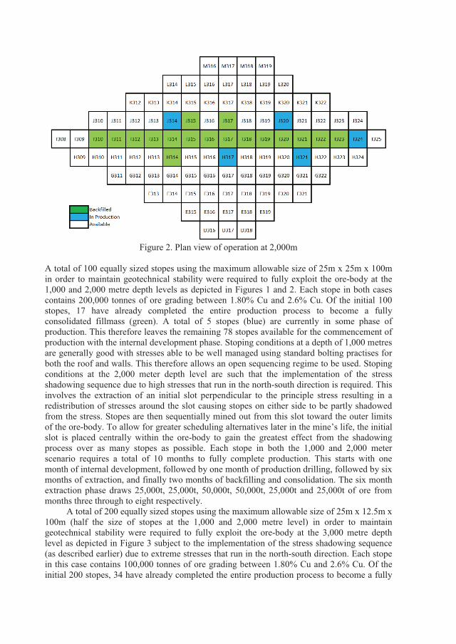
Figure 2. Plan view of operation at 2,000m
A total of 100 equally sized stopes using the maximum allowable size of 25m x 25m x 100m in order to maintain geotechnical stability were required to fully exploit the ore-body at the 1,000 and 2,000 metre depth levels as depicted in Figures 1 and 2. Each stope in both casescontains 200,000 tonnes of ore grading between 1.80% Cu and 2.6% Cu. Of the initial 100 stopes, 17 have already completed the entire production process to become a fully consolidated fillmass (green). A total of 5 stopes (blue) are currently in some phase of production. This therefore leaves the remaining 78 stopes available for the commencement of production with the internal development phase. Stoping conditions at a depth of 1,000 metres are generally good with stresses able to be well managed using standard bolting practises for both the roof and walls. This therefore allows an open sequencing regime to be used. Stoping conditions at the 2,000 meter depth level are such that the implementation of the stress shadowing sequence due to high stresses that run in the north-south direction is required. This involves the extraction of an initial slot perpendicular to the principle stress resulting in a redistribution of stresses around the slot causing stopes on either side to be partly shadowed from the stress. Stopes are then sequentially mined out from this slot toward the outer limits of the ore-body. To allow for greater scheduling alternatives later in the mine’s life, the initial slot is placed centrally within the ore-body to gain the greatest effect from the shadowing process over as many stopes as possible. Each stope in both the 1,000 and 2,000 meter scenario requires a total of 10 months to fully complete production. This starts with one month of internal development, followed by one month of production drilling, followed by six months of extraction, and finally two months of backfilling and consolidation. The six month extraction phase draws 25,000t, 25,000t, 50,000t, 50,000t, 25,000t and 25,000t of ore from months three through to eight respectively.
A total of 200 equally sized stopes using the maximum allowable size of 25m x 12.5m x 100m (half the size of stopes at the 1,000 and 2,000 metre level) in order to maintain geotechnical stability were required to fully exploit the ore-body at the 3,000 metre depth level as depicted in Figure 3 subject to the implementation of the stress shadowing sequence (as described earlier) due to extreme stresses that run in the north-south direction. Each stope in this case contains 100,000 tonnes of ore grading between 1.80% Cu and 2.6% Cu. Of the initial 200 stopes, 34 have already completed the entire production process to become a fully

consolidated fillmass (green). A total of 10 stopes (blue) are currently in some phase of production. This therefore leaves the remaining 156 stopes available for the commencement of production with the internal development phase. Each stope in this case requires a total of 8 months to fully complete production. This starts with one month of internal development, followed by one month of production drilling, followed by four months of extraction, and finally two months of backfilling and consolidation. The four month extraction phase draws 16,666t, 33,333t, 33,333t and 16,666t of ore for months three through to six respectively.
Figure 3. Plan view of operation at 3,000m
Long term production scheduling will be carried out at monthly intervals over the life of the operation. A copper price of $5000/t is used and a discount rate of 10% pa is applied. An operating cost per tonne of ore ($/t) is estimated for each scenario. These estimations were carried out by analysing simulation results and adjusting and extrapolating a set of actual operating costs. The total operating costs (OPEX), the operating cost from haulage options (Haulage OPEX), and the costs from other operations (OPEX Ex. Haulage) are presented in Tables 1 and 2 for the current and three times energy prices respectively.
These operating costs are subtracted from the operating revenues to calculate the undiscounted cash flows associated with the extraction phase of each stope which in turnforms the basis for the production scheduling optimisation process. The only resource constraint that is applicable in this case is related to the targeted ore tonnage to be produced from the operation. Monthly production is therefore limited to be less than or equal to 100,000 tonnes. The main sequencing constraints typically associated with sublevel stoping which are also applicable in this case are:
(1) Continuous Production(2) Non-concurrent adjacent stope production(3) Single backfill exposure(4) Double stope exposure
The other constraint which will require compliance relates to the implementation of the stress shadowing sequence for the 2,000 and 3,000 meter depth levels. This therefore limits when

stopes can enter production due to the respective stope on the outer side of each stope needing to be mined first.
Table 1. Operating cost ($/t) structure at current energy prices
1,000 meters 2,000 meters 3,000 metersEnergy
Component TotalEnergy
Component TotalEnergy
Component Total
Die
sel
truc
k Haulage OPEXOPEX Ex. HaulageTotal OPEX
16.702.20
18.90
26.7022.8049.50
31.603.80
35.40
41.4034.2075.60
104.306.60
110.90
123.8051.90
175.70
Elec
tric
tr
uck Haulage OPEX
OPEX Ex. HaulageTotal OPEX
7.902.10
10.00
14.3021.7036.00
15.203.40
18.60
24.0032.7056.70
52.406.10
58.50
73.2048.30
121.50
Shaf
t Haulage OPEXOPEX Ex. HaulageTotal OPEX
0.901.902.80
6.5019.5026.00
1.903.105.00
9.8028.7038.50
2.905.708.60
12.1043.6055.70
Con
veyo
r
Haulage OPEXOPEX Ex. HaulageTotal OPEX
1.701.903.60
6.8020.0026.80
6.803.109.90
24.0029.8053.80
10.905.80
16.70
33.0045.7078.70
Table 2. Operating cost ($/t) at three times current energy prices
1,000 meters 2,000 meters 3,000 metersEnergy
Component TotalEnergy
Component TotalEnergy
Component Total
Die
sel
truc
k Haulage OPEXOPEX Ex. HaulageTotal OPEX
50.106.60
56.70
60.1027.2083.30
94.8011.40
106.20
104.641.80
146.40
312.9019.80
332.70
332.4065.10
397.50
Elec
tric
tr
uck Haulage OPEX
OPEX Ex. HaulageTotal OPEX
23.706.30
30.00
30.1025.9056.00
45.6010.2055.80
54.4039.5093.90
157.2018.30
175.50
178.0060.50
238.50
Shaf
t Haulage OPEXOPEX Ex. HaulageTotal OPEX
2.705.708.40
8.3023.3031.60
5.709.30
15.00
13.6034.9048.50
8.7017.1025.80
17.9055.0072.90
Con
veyo
r
Haulage OPEXOPEX Ex. HaulageTotal OPEX
5.105.70
10.80
10.2023.8034.00
20.409.30
29.70
37.6036.0073.60
32.7017.4050.10
54.8057.30
112.10

5.1 Model Formulation
To carry out the objectives of this investigation:(1) Simulation will be used to aid in determining the expected operating costs associated
with each haulage option at each depth level across energy price scenario. GPSS/H was used for all simulation.
(2) Once costs have been established these will be used to calculate operating cash flowsassociated with each stope. A Mixed Integer Programming (MIP) production scheduling model which is solved using CPLEX will then be used to carry out optimised production scheduling in order to generate an operating NPV for each scenario.
5.1.1 The simulation model programming
Two models were created for the material flow at different mine depths. The first model involves diesel and electric trucks, and the second is for the shaft and belt conveyor. At each depth diesel and electric trucks are loaded by loaders located at the loading point below the crusher and transport the ore to the stockpile near the process plant at the mine surface. The electric trucks leave the trolley electricity line during loading and dumping and use a small diesel motor. The total haul road distance was 10km at 10% grade. At this grade, the load factor used for empty and full trucks was 0.35 and 0.5 respectively [13].
For shaft modeling, a skip weight of 15 tonnes was considered. This weight is maintained for all mine depths with the variation of rope speed based on the required production rate. Two and three stage shafts were used at 2,000m and 3,000m depths respectively. Four hoist ropes at 26mm flattened strand with sheave diameter of 3.4m was used while the efficiency of the friction hoist was estimated as 90%. The power consumption was calculated based on the horsepower required to move the shaft up and down.
For the belt conveyor, three equal roll idlers at 35° troughing angle was used on the carry and return side. By using a control system the belt speed is controlled or adjusted depending on material flow. The variation of the belt speed leads to a change in the power to drive the motors which also varies the material discharge curves. The total distance covered by the belt was 2,900km, 4,000 km and 6,000 km at 1,000m, 2,000m and 3,000m depths respectively. The power requirement for the belt conveyor is then calculated based on elevation and friction components.
Models were developed using GPSS/H simulation language. In modeling, GPSS/H uses a process interaction approach by specifying sequence of events separated by lapses in time which describes the manner in which transactions flow through a system. Transactions which are created and introduced to a model from time to time, move along the path in a model as simulation proceeds and then leave the model. Positions on the path along which transactions move are called blocks. Each block represents a subroutine. As transaction flow, they automatically queue when the resources are not free to be used. Transactions are created by the GENERATE or START statements and destroyed by the TERMINATE statement. Resources are static permanent entities desirable to substitute a transaction. The variable parameters are described as character, integer, and the floating point data, and can be read using The GETLIST statement and the BGETLIST blocks. Blocks describe how a transaction moves through the system and is processed. A value to the block is assigned by BLET, LET, and SAVEVALUE blocks. Several other GPSS/H blocks were used during modeling. In GPSS/H there are over fifty different types of blocks available which can be used to model complex problems [27]. Complete programming codes were created and the simulation output was generated. Part of the GPSS/H simulation program for diesel and electric trucks is shown
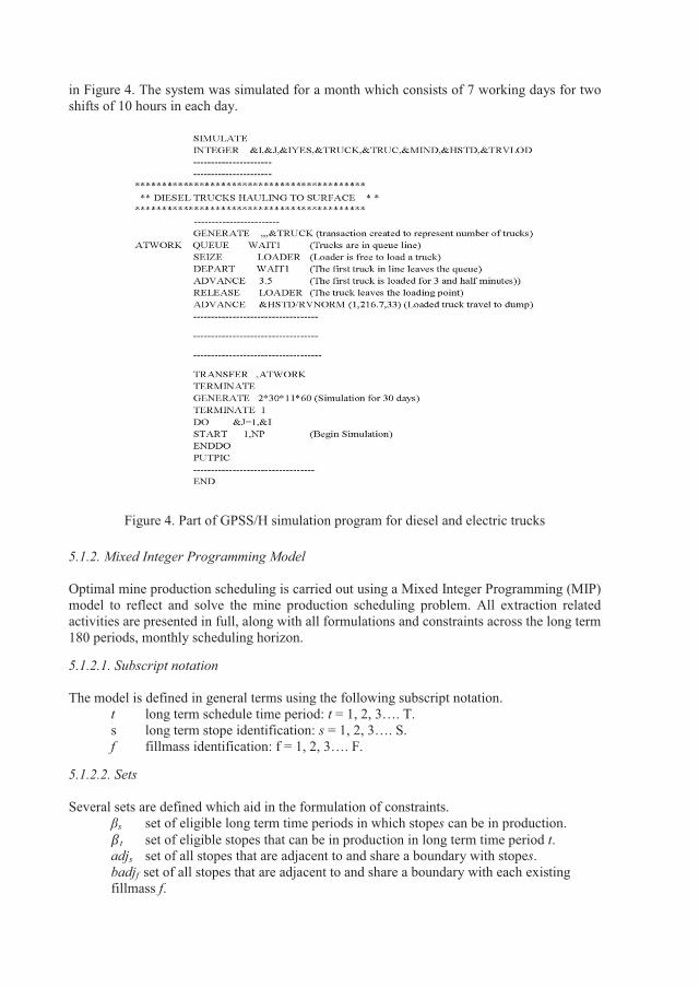
in Figure 4. The system was simulated for a month which consists of 7 working days for two shifts of 10 hours in each day.
Figure 4. Part of GPSS/H simulation program for diesel and electric trucks
5.1.2. Mixed Integer Programming Model
Optimal mine production scheduling is carried out using a Mixed Integer Programming (MIP) model to reflect and solve the mine production scheduling problem. All extraction related activities are presented in full, along with all formulations and constraints across the long term 180 periods, monthly scheduling horizon.
5.1.2.1. Subscript notation
The model is defined in general terms using the following subscript notation.t long term schedule time period: t = 1, 2, 3…. T.s long term stope identification: s = 1, 2, 3…. S.f fillmass identification: f = 1, 2, 3…. F.
5.1.2.2. Sets
Several sets are defined which aid in the formulation of constraints.s set of eligible long term time periods in which stopes can be in production.t set of eligible stopes that can be in production in long term time period t.
adjs set of all stopes that are adjacent to and share a boundary with stopes.badjf set of all stopes that are adjacent to and share a boundary with each existing fillmass f.

tpbt set of time periods that include all periods up to the current period t.
5.1.2.3. Parameters
These parameter items represent the numeric inputs and conditions.nt present value discount factor for time period t.cfs undiscounted cashflow ($) from each stopes.es earliest start time for stopes.ls latest start time for stopes.rs extraction reserve (t) for each stopes.sct shaft/LHD/truck fleet movement capacity (t) for each time period t.
5.1.2.4. Decision variables
One binary variable was required to reflect operating conditions and ultimately perform the scheduling task.
wst 1 if production from stopes is scheduled for time period t,0 otherwise.
5.1.2.5. Objective function
The objective function seeks to maximise the NPV of all activities under consideration by determining the optimal schedule within which to progress each stope through production.
:
,
× × (7)
It should be noted that taxation and depreciation are not included in this formulation.However these should be incorporated if necessary.
5.1.2.6. Constraints
The production scheduling model comprises numerous constraints which reflect the practical limitations imposed by the sublevel stoping method over the long term scheduling horizon.These constraints can be classified according to the limitations they impose on resources, sequencing and timing.
5.1.2.7. Resource constraints
The following formulations display the mathematical resource constraints that are applicable across the long term horizon.
Shaft / machine fleet ore capacity constraint× (8)
Non-negativity and integer value constraint = (9)

Constraint (8) limits production of all development and stope extraction ore from exceeding the shaft/LHD/truck fleet capacity in any long term time period. Constraint (9) enforces non-negativity and integer values of the appropriate variables.
5.1.2.8. Sequencing constraints
The following formulations display the mathematical sequencing constraints that are applicable across the long term horizon.
Stope production precedence sequencing constraint , | (10)
Non-concurrent stope sequencing constraint+ 1 , | (11)
Stope adjacency constraint+ 1 , | (12)
Fillmass adjacency constraint+ 2 , (13)
Existing fillmass adjacency constraint1 , (14)
All proceeding production sequencing between stopes also enforced by constraints (10) and (11). Constraint (12) ensures that simultaneous production between stopes that share a common boundary does not occur. Constraint (13) provides some geotechnical stability to stoping activities by limiting simultaneous adjacent production to two common boundaries before itself commencing production, and to a single adjacent side once having completed production to become a fillmass. Constraint (14) ensures fillmass stability of all existing fillmasses by limiting exposure to a single common boundary in each long term time period.
5.1.2.9. Timing constraints
The following formulations display the mathematical timing constraints that are applicableacross the long term horizon.
May mine constraint1 | > (15)
Must mine constraint = 1 | (16)
Constraint (15) ensures that commencement of stope production is initiated no more than once during the long term scheduling horizon if their late start date occurs beyond the scheduling

horizon. Constraint (16) requires stope production commences at some point during the longterm scheduling horizon if their late start date falls within the long term scheduling horizon.
6. Results and discussion
6.1. Simulation results
The first created simulation model involves diesel and electric trucks to simulate the fleet required to achieve a monthly production target of 100,000 tonnes. The results show that, although the size of electric truck is 2 tonnes smaller than that of diesel truck, the number of trucks required to achieve the production target at 1,000m depth were 7 and 5 for diesel and electrical respectively. This is because the complete cycle time of the electric truck is shorter than the diesel truck which allows more cycles to be done within the same period of time. The simulation was repeated for the depths of 2,000m and 3,000m and the results shows that more diesel trucks than electric truck are required to achieve the same output.
The second model combined shaft and conveyor systems. The results indicated that when the depth is at 1000m, a shaft system of two skips in balance each of 15 tonnes can haul 100,000 tonnes of ore at a speed of 8.5m/s. The simulation was repeatedly run with the same skip size and variable rope speeds. The results show that rope speeds were increased to 10m/s and 14m/s to haul material from 2000m to 1000m, and from 3000m to 2000m respectively.The conveyor belt hauls the ore from the storage bin located under the underground crusher to a stockpile on the surface. The initial belt width and speed shows that the belt conveyor can haul 80tons/hour. During model programming it was assumed that there were no belt conveyor breakdown, this is because there is no reliability data available for this study. The program assumes that there is no restriction on the ore bin capacity as the belt can haul all the ore as it enters the bin. During simulation, belt width and speed were raised to accommodate the planned production. The simulation was repeated for the 2000m and 3000m depths and the energy required to haul material is then determined. The simulation results obtained from all haulage options were used in the determination of the energy cost per tonne of ore for each haulage scenario and then exported to the mixed integer programming model for optimization purposes.
6.2. Mixed Integer Programming results
Construction of all Mixed Integer Programming (MIP) models for the purpose of optimal production scheduling (maximize NPV) was done using A Mathematical Programming Language (AMPL), based on the costs and parameters mentioned earlier, and they were then solved using CPLEX version 10.3. The solution process for each of the 24 scenarios was left to run for approximately 10 hours and was cut short even if convergence to the optimal solution had not yet been achieved. In all cases however, a gap of less than 5% was achieved. Production scheduling took place at monthly intervals and was limited to 180 periods (15 years). In some cases, especially in the open sequencing regime at the 1,000 meter level, full extraction was completed earlier than the 180 month limit, while in the highly constrained cases this did not result in the full extraction of all stopes.
The operating NPVs that were achieved from each of the 24 scenarios are shown in Figures 5 and 6. As shown, the operating costs for diesel trucks together with increasing sequencing constraints with increasing depth, results in lower operating NPVs and an unfeasible operation at current and three times current energy prices compared to electric truck, shaft, and conveyor belt haulage systems for all depth levels. While diesel truck haulage generally offers greater operational flexibility, its high energy intensity results in a
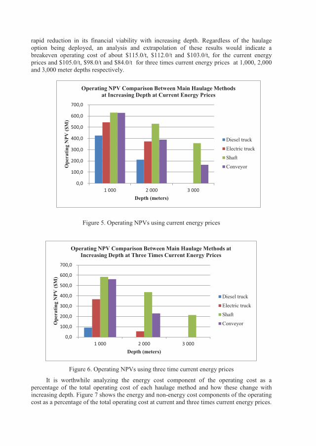
rapid reduction in its financial viability with increasing depth. Regardless of the haulage option being deployed, an analysis and extrapolation of these results would indicate abreakeven operating cost of about $115.0/t, $112.0/t and $103.0/t, for the current energy prices and $105.0/t, $98.0/t and $84.0/t for three times current energy prices at 1,000, 2,000 and 3,000 meter depths respectively.
Figure 5. Operating NPVs using current energy prices
Figure 6. Operating NPVs using three time current energy prices
It is worthwhile analyzing the energy cost component of the operating cost as a percentage of the total operating cost of each haulage method and how these change with increasing depth. Figure 7 shows the energy and non-energy cost components of the operating cost as a percentage of the total operating cost at current and three times current energy prices.
0,0
100,0
200,0
300,0
400,0
500,0
600,0
700,0
1 000 2 000 3 000
Ope
ratin
g N
PV ($
M)
Depth (meters)
Operating NPV Comparison Between Main Haulage Methods at Increasing Depth at Current Energy Prices
Diesel truck
Electric truck
Shaft
Conveyor
0,0
100,0
200,0
300,0
400,0
500,0
600,0
700,0
1 000 2 000 3 000
Ope
ratin
g N
PV ($
M)
Depth (meters)
Operating NPV Comparison Between Main Haulage Methods at Increasing Depth at Three Times Current Energy Prices
Diesel truck
Electric truck
Shaft
Conveyor
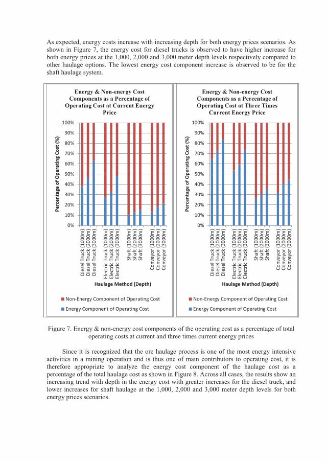
As expected, energy costs increase with increasing depth for both energy prices scenarios. As shown in Figure 7, the energy cost for diesel trucks is observed to have higher increase for both energy prices at the 1,000, 2,000 and 3,000 meter depth levels respectively compared to other haulage options. The lowest energy cost component increase is observed to be for the shaft haulage system.
Figure 7. Energy & non-energy cost components of the operating cost as a percentage of total operating costs at current and three times current energy prices
Since it is recognized that the ore haulage process is one of the most energy intensive activities in a mining operation and is thus one of main contributors to operating cost, it is therefore appropriate to analyze the energy cost component of the haulage cost as a percentage of the total haulage cost as shown in Figure 8. Across all cases, the results show an increasing trend with depth in the energy cost with greater increases for the diesel truck, and lower increases for shaft haulage at the 1,000, 2,000 and 3,000 meter depth levels for both energy prices scenarios.
0%
10%
20%
30%
40%
50%
60%
70%
80%
90%
100%
Dies
el T
ruck
(100
0m)
Dies
el T
ruck
(200
0m)
Dies
el T
ruck
(300
0m)
Elec
tric
Tru
ck (1
000m
)El
ectr
ic T
ruck
(200
0m)
Elec
tric
Tru
ck (3
000m
)
Shaf
t (10
00m
)Sh
aft (
2000
m)
Shaf
t (30
00m
)
Conv
eyor
(100
0m)
Conv
eyor
(200
0m)
Conv
eyor
(300
0m)
Perc
enta
ge o
f Ope
ratin
g Co
st (%
)
Haulage Method (Depth)
Energy & Non-energy Cost Components as a Percentage of
Operating Cost at Current Energy Price
Non-Energy Component of Operating Cost
Energy Component of Operating Cost
0%
10%
20%
30%
40%
50%
60%
70%
80%
90%
100%
Dies
el T
ruck
(100
0m)
Dies
el T
ruck
(200
0m)
Dies
el T
ruck
(300
0m)
Elec
tric
Tru
ck (1
000m
)El
ectr
ic T
ruck
(200
0m)
Elec
tric
Tru
ck (3
000m
)
Shaf
t (10
00m
)Sh
aft (
2000
m)
Shaf
t (30
00m
)
Conv
eyor
(100
0m)
Conv
eyor
(200
0m)
Conv
eyor
(300
0m)
Perc
enta
ge o
f Ope
ratin
g Co
st (%
)
Haulage Method (Depth)
Energy & Non-energy Cost Components as a Percentage of Operating Cost at Three Times
Current Energy Price
Non-Energy Component of Operating Cost
Energy Component of Operating Cost
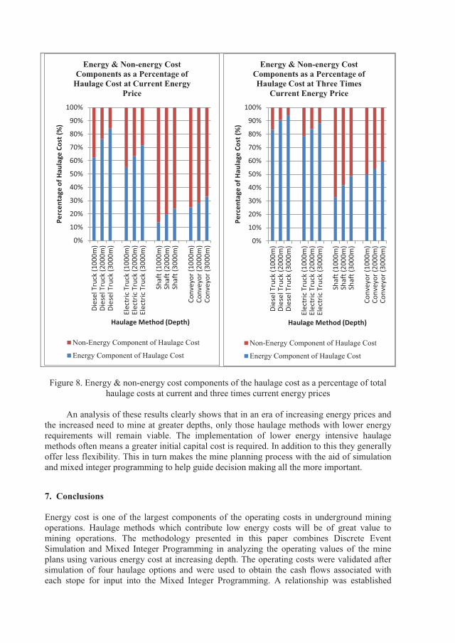
Figure 8. Energy & non-energy cost components of the haulage cost as a percentage of total haulage costs at current and three times current energy prices
An analysis of these results clearly shows that in an era of increasing energy prices and the increased need to mine at greater depths, only those haulage methods with lower energy requirements will remain viable. The implementation of lower energy intensive haulage methods often means a greater initial capital cost is required. In addition to this they generally offer less flexibility. This in turn makes the mine planning process with the aid of simulation and mixed integer programming to help guide decision making all the more important.
7. Conclusions
Energy cost is one of the largest components of the operating costs in underground mining operations. Haulage methods which contribute low energy costs will be of great value to mining operations. The methodology presented in this paper combines Discrete Event Simulation and Mixed Integer Programming in analyzing the operating values of the mine plans using various energy cost at increasing depth. The operating costs were validated after simulation of four haulage options and were used to obtain the cash flows associated with each stope for input into the Mixed Integer Programming. A relationship was established
0%
10%
20%
30%
40%
50%
60%
70%
80%
90%
100%
Dies
el T
ruck
(100
0m)
Dies
el T
ruck
(200
0m)
Dies
el T
ruck
(300
0m)
Elec
tric
Tru
ck (1
000m
)El
ectr
ic T
ruck
(200
0m)
Elec
tric
Tru
ck (3
000m
)
Shaf
t (10
00m
)Sh
aft (
2000
m)
Shaf
t (30
00m
)
Conv
eyor
(100
0m)
Conv
eyor
(200
0m)
Conv
eyor
(300
0m)
Perc
enta
ge o
f Hau
lage
Cos
t (%
)
Haulage Method (Depth)
Energy & Non-energy Cost Components as a Percentage of
Haulage Cost at Current Energy Price
Non-Energy Component of Haulage Cost
Energy Component of Haulage Cost
0%
10%
20%
30%
40%
50%
60%
70%
80%
90%
100%
Dies
el T
ruck
(100
0m)
Dies
el T
ruck
(200
0m)
Dies
el T
ruck
(300
0m)
Elec
tric
Tru
ck (1
000m
)El
ectr
ic T
ruck
(200
0m)
Elec
tric
Tru
ck (3
000m
)
Shaf
t (10
00m
)Sh
aft (
2000
m)
Shaf
t (30
00m
)
Conv
eyor
(100
0m)
Conv
eyor
(200
0m)
Conv
eyor
(300
0m)
Perc
enta
ge o
f Hau
lage
Cos
t (%
)
Haulage Method (Depth)
Energy & Non-energy Cost Components as a Percentage of Haulage Cost at Three Times
Current Energy Price
Non-Energy Component of Haulage Cost
Energy Component of Haulage Cost

showing how energy costs increase with increasing mine depth for both current and three times energy prices. It was shown that the increase in energy cost associated with diesel truck is substantially higher compared to other haulage options. The investigation provides mining operations with a preliminary assessment of the energy costs associated with various haulage methods as mine depth increases for the purpose of aiding the decision making process in regard to future deeper underground mining. Deposits are analyzed by using metal grades to establish revenues with each resource block based on an assumed metal price. Uncertainties associated with metal prices and grade block model will occur over the life of any operation. This leads to a new block value which result in generating a new mine plan. The uncertainty related to metal price and grade was not included in this study. Future work may therefore involve conditional simulation to measure the sensitivity to some of these uncertainties.
Acknowledgements
The authors would like to acknowledge the efforts of personnel from the Division of Mining and Geotechnical Engineering at Luleå University of Technology, and the School of Mechanical and Mining Engineering at The University of Queensland whose collaborating efforts made this project possible. Also the authors would like to thank I2Mine project within the EU 7th framework programme for funding parts of the work.
References
[1] V. Kecojevic and D. Komljenovic,Haul truck fuel consumption and CO2 emission under various engine load conditions. Mining Engineering. 62(12) (2010), ProQuest Central, pp. 44-48.
[2] Environmental Protection Agency (EPA), Average carbon dioxide emission resulting from gasoline and diesel fuel. Office of Transportation and air quality, Washington DC, 2005.
[3] N. Thomas, A.J Gregg, and H.L Hartman, Comparative performance study of diesel and electric face-haulage vehicles. Int. J. Mining.Geologic.Eng., 5(1987), pp. 405-417
[4] F.E Scott, Diesels underground overcoming a bad image, Coal mining and processing,19 (8) (1982), pp. 45-51.
[5] J. Hiltermann, G. Lodewijks, D.L. Schott, J.C Rijsenbrij, J. A.J.M. Dekkersand Y. Pang, A Methodology to Predict Power Savings of Troughed Belt Conveyors by Speed Control, Particulate Science and Technology, Int. J. Mining. Reclam. Environ., 29(1)(2011), pp. 14-27.
[6] J.R Sturgul and Li, New development in simulation technology and applications in the mineral industry, Int. J. Mining. Reclam. Environ. 11(4) (1997), pp. 159-162.
[7] Goodyear and Rubber company, Handbook of Conveyor &Elevator belting, Akron, Ohio 44316, USA, (1976), Chap. 6, pp. 1-8.
[8] G. Beerkircher, Mine hoists: Underground mining methods handbook, in SME, chap. 5.5, USA, (1989), pp. 1386-1403.
[9] J.H Harmon, Hoist and hoisting systems, in SME, Chap 15. SME-AIME, New York,(1973), pp. 15-59.
[10] Anon, Procedures for Hoist and shaft inspection and maintenance. Vol I and II, USBM, PB83-148049 and PB83-148056, Washington DC, 1981b.
[11] M. Hager and A. Hintz, The Energy-Saving design of belts for long conveyor systems,Bulk Solids Handling, 13(4) (1993), pp. 749-758.
[12] R.T Swinderman, The conveyor drives power consumption of belt cleaners. , Bulk Solids Handling, 11(1991), pp. 487.
[13] Caterpillar, Caterpillar performance handbook, Edition 39, Caterpillar Inc., Peoria, IL, (2009).
[14] http://www.i2mine.eu/, Accessed on 27th August 2012[15] C. Alford, Optimisation in underground mine design, 25th Int. APCOM. Symposium,
Australian Instit. Mining and Metallurgy: Melbourne, (1995), pp. 213-218.[16] M. Ataee-Pour, A critical survey of existing stopes layout optimisation techniques, J.
Mining. Science, Springer: New York, (2005), pp. 447-466.[17] M. Brazil and D.A Thomas, Network optimisation for the design of underground
mines, Inter Science, John Wiley and Sons Inc.New Jersey, (2004).[18] M. Carlyle and B.C Eaves, Underground planning at Stillwater Mining Company,
Interfaces. Springer: New York, (2001), pp. 50-60.[19] F. S. Hillierand G. J. Lieberman, Introduction to operations research, Boston, Mass,
McGraw Hill, (2001).[20] J. Little, A new approach to using mixed-integer programming for scheduling
optimisation in sublevel stope mining, Bsc. Diss., Queensland University, (2007).[21] G. McIsaac, Long-term planning of an underground mine using mixed-integer linear
programming, CIM Bulletin,Canad. Inst. Mining.Metal. Petroleum, Westmount, (2005).
[22] M. Nehring, E. Topal, M. Kizil and P. Knights, Integrated short- and medium-term underground mine production scheduling.J.South. African Inst.Mining.Metall, 112(5)(2012), pp. 365-378.
[23] M. Nehring, E. Topal and J. Little, A new mathematical programming model for production schedule optimization in underground mining operations, J.South. AfricanInst.Mining.Metall, 110(8) (2010), pp. 437-446.
[24] M. Nehring, E. Topaland P. Knights, Dynamic Short term production scheduling and machine allocation in underground mining using mathematical programming,Transactions.Inst. Materials.Minerals. Mining, Section A: Mining. Tech, 119(4)(2010), pp. 212-220.
[25] E. Topal, Early start and late start algorithms to improve the solution time for long-term underground mine production scheduling, J.South. African Inst.Mining.Metall,(2008)
[26] W.L Winston, and J.B Goldberg, Operations research: applications and algorithms,Thomson: Belmont, (2004).
[27] T. Schriber, Perspectives on simulation using GPSS, in Proc. Winter. Simulation, M. Abrams, ed., Soc. Comp Sim, Publisher, San diego, CA, (1988).
[28] J. Harrison and J.R Sturgul, GPSS Computer simulation of equipment requirements for the iron duke mine, Second large open pit mining conference, Melbourne, Vie., AusIMM, (1989), pp. 133-136.
[29] J.R Sturgul and R. Singhal, Using the personal computer to simulate mining operations, in Proc Computer. Applic.Mineral. Industry (CAMI), Laval University, Quebec city, Balkema, Publisher, Rotterdam, (1988), pp. 439-442.
[30] J.R Sturgul, Discrete mine system simulation in the United states, Int. J. Mining.Reclam. Environ. 13(2) (1999), pp. 37-41.
[31] G.N. Panagiotou, Discrete mine system simulation in Europe, Int. J. Mining.Reclam. Environ. 13(2) (1999), pp. 43-46.
[32] J.P.I Ketelaar and P.J Davidson, Improving the efficiency of conveyors used for the transport of minerals in underground and surface mines, Mining Tech, 77(883), (1995).


