Lidar Investigation of Atmosphere Effect on a Wind Turbine ...

Lidar Investigation of Atmosphere Effect on a Wind Turbine Wake

I. N. SMALIKHO AND V. A. BANAKH

V. E. Zuev Institute of Atmospheric Optics, Siberian Branch, Russian Academy of Sciences, Tomsk, Russia

Y. L. PICHUGINA, W. A. BREWER, AND R. M. BANTA

NOAA/Earth System Research Laboratory, Boulder, Colorado

J. K. LUNDQUIST AND N. D. KELLEY

National Renewable Energy Laboratory, Golden, Colorado

(Manuscript received 17 May 2012, in final form 9 February 2013)

ABSTRACT

An experimental study of the spatial wind structure in the vicinity of a wind turbine by a NOAA coherent

Doppler lidar has been conducted. It was found that a working wind turbine generates a wake with the

maximum velocity deficit varying from 27% to 74% and with the longitudinal dimension varying from 120 up

to 1180m, depending on the wind strength and atmospheric turbulence. It is shown that, at high wind speeds,

the twofold increase of the turbulent energy dissipation rate (from 0.0066 to 0.013m2 s23) leads, on average, to

halving of the longitudinal dimension of the wind turbine wake (from 680 to 340m).

1. Introduction

As awind turbine operates, a fraction of the wind-flow

energy is transferred to rotate the turbine blades; there-

fore, a wind-velocity deficit is generated downwind of the

turbine. Studies on the influence of atmospheric conditions

(in particular, wind velocity andwind turbulence intensity)

on the length of a wind wake and the velocity deficit inside

the wake are needed because of the increasing number of

wind farms and the need to optimize the turbine ar-

rangement in a wind farm.

Flow characteristics behind wind turbines have been

studied extensively during the last three decades. The

most comprehensive review of the theoretical and ex-

perimental studies is provided by Vermeer et al. (2003),

wherein investigations of the wind turbine wake were

conducted through the use of various techniques.

H€ogstr€om et al. (1987) employed four different tech-

niques for probing the turbine wake: 1) tower-mounted

instrumentation, 2) Tala Inc. kite anemometers, 3) teth-

ered balloon soundings, and 4) Doppler sodar. Using

these instruments, the velocity deficit and the turbulence

characteristics in the wind turbine wake were investi-

gated. Using data measured by wind and temperature

sensors at two meteorological masts, Magnusson and

Smedman (1996) derived analytical expressions for the

velocity deficit and the added turbulence of the flow

generated by the wind turbines. Measurement results

of the velocity deficit with a ship-mounted sodar were

compared with this empirical model in Barthelmie et al.

(2003) and with other models in Barthelmie et al. (2006).

A coherent Doppler lidar system (CDL) is a powerful

tool that can measure wind, turbulence, and aircraft

wake vortices (K€opp et al. 1984; Hall et al. 1984; Hawley

et al. 1993; Frehlich et al. 1994, 1998; Banakh et al. 1999;

K€opp et al. 2005; Smalikho et al. 2005; Banta et al. 2006;

Frehlich et al. 2006; Pichugina et al. 2008; Rahm and

Smalikho 2008; Banakh et al. 2009; Pichugina and Banta

2010; O’Connor et al. 2010). Results of a study of the

wake generated by a wind turbine with the aid of a

continuous-wave CDL are presented in papers by Bing€ol

et al. (2010) and Trujillo et al. (2011). During the exper-

iment, the lidar was located at the rear of the nacelle, and

the laser beam scans were used to measure wind turbine

wake dynamics and investigate the influence of different

turbulence scales on the wake behavior. For a continuous-

wave CDL, the longitudinal size of the sensing volume

Corresponding author address: Igor N. Smalikho, V. E. Zuev

Institute of Atmospheric Optics, SB RAS, 1 Academician Zuev

Square, Tomsk 634021, Russia.

E-mail: [email protected]

2554 JOURNAL OF ATMOSPHER IC AND OCEAN IC TECHNOLOGY VOLUME 30

DOI: 10.1175/JTECH-D-12-00108.1

� 2013 American Meteorological SocietyUnauthenticated | Downloaded 12/07/21 04:56 AM UTC

increases quickly with the increase of the focal length or

range (Sonnenschein and Horrigan 1971). In the case of

a pulsed CDL, the longitudinal size of the sensing vol-

ume does not depend on the range, and the radial ve-

locities are measured at different ranges along the axis

of the sensing beam as the pulse propagates outward and

interacts with backscattering targets, generally atmo-

spheric aerosol particles. Therefore, pulsed CDL opens

up a wide range of possibilities to investigate the wind

turbine wake, by using the geometry of scanning by the

sensing beam during the measurement time, as was dem-

onstrated by K€asler et al. (2010).

This paper describes the lidar data processing pro-

cedures that were performed to obtain information about

the wind, turbulence, and wind turbine wake, and pres-

ents some results of a field experiment [described in detail

in Lundquist et al. (2013), manuscript submitted to En-

viron. Res. Lett.] that was conducted with the use of a

2-mm pulsed CDL under various atmospheric conditions.

2. Estimation of the dissipation rate of turbulentenergy from scanning CDL data

The use of conical scanning by a sensing beam of the

coherent Doppler lidar around the vertical axis at a fixed

elevation angle u allows researchers to obtain infor-

mation about wind direction and velocity. If measure-

ments are conducted by a pulsed CDL, then the vertical

profiles of these parameters can be retrieved from the

data obtained for one full scan (azimuth angle u varies

from 08 to 3608) using the velocity–azimuth display

(VAD) technique (Browning and Wexler 1968; Banta

et al. 2002). For the continuous-wave CDL, Banakh

et al. (1999) showed that the wind speed and direction

and the turbulence energy dissipation rate within the

atmospheric boundary layer can be estimated from data

measured by conical scanning. In addition, Frehlich

et al. (2006) showed that information about wind tur-

bulence can be retrieved from pulsed CDL data that are

obtained by conical-sector scanning; that is, scanning

in azimuth over a limited sector. We present a brief de-

scription of the approaches used to estimate the turbu-

lence energy dissipation rate « from the transverse and

longitudinal structure functions of the radial velocity, as

measured by a 2-mm pulsed CDL using conical scanning

techniques (including one full scan and multiple sector

scanning).

The Doppler lidar used in this study was the National

Oceanic and Atmospheric Administration’s (NOAA’s)

high-resolution Doppler lidar (HRDL), as described by

Grund et al. (2001). Themain characteristics of this lidar

are given in Table 1. In this table, we also included re-

sults of numerical simulation at weak (sV 5 0.2m s21,

LV 5 100m) and strong (sV 5 1.2m s21, LV 5 100m)

wind turbulence and at different signal-to-noise ratios

(SNRs, the ratio of the mean signal power to the mean

noise power in the spectral bandwidth of 50MHz) for the

error of lidar estimate of the radial velocity (Smalikho

et al. 2013).

Consider the case of a 2-mm pulsed CDL, where the

temporal power profile of the sensing radiation is well

described by aGaussian distribution with pulse duration

2sP, determined from the power drop to the e21 level

from the peak. The pulse repetition frequency is de-

noted FP. During measurements by this lidar, conical

scanning with a constant angular rate v0 is used. For

different distances zi from the lidar and azimuth angles

um, raw data measured by the lidar are used to calculate

the Doppler spectra with the use of the rectangular time

window of width Tw for each spectrum and the accu-

mulation of individual estimates of spectra fromNa lidar

shots, where zi 5 z0 1 iDR, i5 0, 1, 2, . . . , I2 1, z0 � Dp,

TABLE 1. Parameters of HRDL and accuracy of radial velocity estimate.

Wavelength 2.0218mm (Tm: Lu, YAG)

Pulse energy 1.5mJ

Pulse duration (full width at half maximum) 200 ns

Pulse repetition rate 200Hz

Local–slave oscillator frequency offset 100MHz

Telescope diameter 20 cm

Data acquisition Base band (each IQ signal is 0–25MHz);

sampling rate (length) is 50MHz (3m)

Minimum range 189m

Radial velocity sampling (along line of site) 30m

Error of radial velocity estimate at Na 5 100

with probability of bad estimate

(uniformly distributed from 225 to

125m s21) less than 1024

SNR (dB) se [weak turbulence (m s21)] se [strong turbulence (m s21)]

10 0.07 0.15

0 0.1 0.17

210 (at range ;1.5–2 km) 0.38 0.42

NOVEMBER 2013 SMAL IKHO ET AL . 2555

Unauthenticated | Downloaded 12/07/21 04:56 AM UTC

Dp5 csP/2, c is the speed of light, DR5 cTW /2, um 5u0 1mDu, m5 0, 1, 2, . . . ,M2 1, and Du5v0Na/FP.

Then, the centroid of the spectral distribution is used

to estimate the radial velocity (projection of the wind-

velocity vector to the axis of the sensing beam) Vr(zi, um)

with an allowance made for the Doppler relation. If the

estimate is unbiased (where the probability of a bad

estimate caused by the system noise with an allowance

for theDoppler relation is equal to zero), then Vr(zi, um)

can be represented in the following form by averaging

over the azimuth angle (Banakh and Smalikho 1997;

Frehlich and Cornman 2002):

Vr(zi, um)5Vr(zi, um)1Ve(zi, um) , (1)

where

Vr(zi, um)

5N21a �

Na

k51

ð1‘

2‘dz0Qs(z

0)Vr(zi 1 z0, um21 1kv0/FP)

(2)

is the radial velocity averaged over the sensing volume,

Qs(z0)5

1

2DR

�erf

�z0 1DR/2

Dp

�2 erf

�z02DR/2

Dp

��(3)

is the weight function of averaging along the axis

of propagation of the sensing beam, erf(x)5(2/

ffiffiffiffip

p)Ð x0 dj exp(2j2) is the standard error function,

Vr(z0, u) is the radial velocity at the point z0S(u) of

the Cartesian coordinate system fz, x, yg, S(u)5 fsinu,cosu cosu, cosu sinug, and Ve(zi, um) is the random error

of the estimation. This error has the following properties:

hVei50,hVrVei5hVrihVei50,andhVe(zi, um)Ve(zi, ul)i5s2edm2l, where the angular brackets denote averaging

over the ensemble of realizations, s2e 5 hV2

e i is the

variance of the random error of estimation of the

radial velocity, and dm2l is the Kronecker delta

(d0 5 1, dm6¼l 5 0). The integral correlation scale Le 5s22e

Ð ‘0 dz0hVe(zi 1 z0, um)Ve(zi, um)i is determined by

the longitudinal dimension of the sensing volume

Dz5 DR/erf[DR/(2Dp)] (Banakh and Smalikho 1997).

Assuming that the pulse repetition frequency Fp is

high and the conditions Na � 1 and zi � LV are true,

whereLV is the integral scale of correlation of turbulent

fluctuations of the wind velocity (Smalikho et al. 2005),

we transformed the velocity Vr from the polar co-

ordinate system fz0, ug to the rectangular coordinate

system on the plane fz0, y0g (z0 is the longitudinal co-

ordinate axis and y0 is the transverse axis) and, re-

placing the summation with integration in Eq. (2), we

obtained the equation

Vr(zi, ym)

5Dy21

ðDy/22Dy/2

dy0ð1‘

2‘dz0Qs(z

0)Vr(zi 1 z0, ym 1 y0) ,

(4)

where ym 5 y0 1mDy and Dy5 ziDu cosu. This approx-imation is rigorous under the conditions mDy/(zi cosu) � p/2 and z0 � iDR.

a. Transverse structure function

For the case of statistically homogeneous and iso-

tropic turbulent flow, we obtained from Eqs. (1)–(4) an

equation for the transverse structure function of the

radial wind velocity measured by Doppler lidar for

azimuthal scanning, DV(mDy)5 h[Vr0(zi, y0 1mDy)2

Vr0(zi, y0)]

2i (Vr0 5 Vr 2 hVri) in the form

DV(mDy)5DV(mDy)1 2(12 dm)s2e , (5)

where

DV(mDy)5 8

ð‘0dkz

ð‘0dky SV(kz, ky)Hz(kz)Hy(ky)[12 cos(2pmDyky)] (6)

is the transverse structure function of the radial velocity

averaged over the sensing volume, SV(kz,ky) is the two-

dimensional spatial spectrum of turbulent fluctuations

of the wind velocity,

Hz(kz)5 fexp[2(pDpkz)2] sinc(pDRkz)g2 (7)

is the function of the low-pass filter along the axis z0, and

Hy(ky)5 sinc2(pDyky) (8)

is the function of the low-pass filter along the axis y0,sinc(x)5 sin(x)/x. For the von K�arm�an model (Monin

and Yaglom 1975; Vinnichenko et al. 1973)



SV(kz,ky)5 0:008 15CK«2/3

"(8:42LV)

2

11 (8:42LV)2(k2z1 k2y)

#4/3

3

"11

8

3

(8:42LVky)2

11 (8:42LV)(k2z1 k2y)

#,

(9)

whereCK ’ 2 is the Kolmogorov constant. The variance

of wind velocity s2V 5 hV2

r i2 hVri2 is related to « and LV

by the equation:

s2V 5 0:636CK(«LV)

2/3 . (10)

Because the difference DDV(mDy)5DV(mDy)2DV(Dy) does not depend on the errorse [seeEq. (5)], from

the measured transverse structure function of radial ve-

locity DV(mDy), estimates of the turbulence energy dissi-

pation rate « and the integral scale LV can be obtained

using the following algorithm (Smalikho andBanakh2013):

min[r(LV)]5 r(LV) (11)

and

«5 [m(LV)]3/2 , (12)

where

r(LV)5 �M0

m52

2664 DDV(mDy)

G(mDy;LV)2m(LV)

37752

,

m(LV)51

M02 1�N

n52

DDV(mDy)

G(mDy;LV),

DDV(mDy) 5 DV(mDy) 2 DV(Dy), G(mDy;LV) 5[DV(mDy)2DV(Dy)]/«

2/3, and M0Dy. 2LV . The func-

tion G(mDy;LV) was calculated using Eqs. (6)–(9).

Then, using estimates « and LV , the wind-velocity vari-

ance s2V was calculated by Eq. (10).

In contrast to the approach of Frehlich et al. (2006),

we used calculations of DV(mDy) to take into account

the averaging of the radial velocity across the probing

beams (along the axis y0). We used such an approach

because, in our experiments at large ranges Ri, the

transverse distance Dy between successive lidar beams,

which is proportional to Du, can exceed the longitudinal

size Dz of the sensing volume.

b. Longitudinal structure function

As the measurement range zi increases, the transverse

dimension of the sensing volume Dy5 ziDu cosu in-

creases as well. However, the condition z0 � iDR allows

us to use the approximation Dy ’ [z0 1 DR(I 2 1)/2]

Du cosu in Eq. (4). That is,Dy can be considered constantalong the propagation path. Then, for the longitudinal

structure function of the radial velocity measured by the

lidar DV(iDR)5 h[Vr0(z0 1 iDR, ym)2Vr

0(z0, ym)]2i, we

obtain from Eqs. (1)–(4)

DV(iDR)5DV(iDR)1 2s2

e[12Ke(iDR)] , (13)

where

DV(iDR)5 8

ð‘0dkz

ð‘0dky SV(kz, ky)Hz(kz)Hy(ky)[12 cos(2piDRkz)] . (14)

From the measured transverse structure function of

radial velocity DV(iDR), estimates of the turbulence

parameters «, LV , and s2V can be obtainedwith the use of

Eqs. (7)–(10) and (14) and the approaches described

in the works of Frehlich and Cornman (2002) and

Smalikho et al. (2005).

c. Comparison of vertical « profiles: Lidar techniqueversus sonic anemometer

To test the method of estimation of « from lidar

measurements of the transverse structure function

DV(mDy), we used data from the experiment conducted

in September 2003 in southeastern Colorado within the

framework of the Lamar Lower-Level Jet Project

(Banta et al. 2006; Kelley et al. 2007; Pichugina and

Banta 2010). In this experiment, HRDL was operated

along with four sonic anemometers installed on a 120-m

meteorological tower (at heights of 54, 67, 85, and

116m). The distance between the tower and the HRDL

container was 167m. For the comparative analysis of the

results of joint measurements of the dissipation rate « by

HRDL and sonic anemometers, we selected the initial

experimental data obtained on 15 September 2003,

when thewind directionwas such that wind-flowdistortion

effects introduced by the meteorological tower on the

sonic anemometer measurements could be neglected.

During the HRDL measurements, different scanning

geometries were used. In the work of Banakh et al.



(2009), we applied the raw experimental wind data ob-

tained on 15 September 2003 and conducted a compar-

ative analysis of the « estimation from the longitudinal

structure function of the radial velocity measured by

HRDL scanning in the vertical plane and from temporal

spectra of the wind velocity measured by sonic ane-

mometers. In that case, the resolution in the scanning

angle was 0.258 and the transverse dimension of the

sensing volume Dy was much smaller than the longitu-

dinal dimension Dz ; 40m out to the measurement

range zi 5 3 km. Because of this condition, the theo-

retical calculations of the longitudinal structure function

by Banakh et al. (2009) were able to neglect the aver-

aging of turbulent fluctuations of the velocity along the

transverse coordinate, in contrast to Eq. (14). As a result

of the analysis of « estimated from lidar data, compared

with that from sonic anemometer data measured for

a;16-min period (Smalikho 1997), Banakh et al. (2009)

found that the relative error of the lidar estimation of «

did not exceed 25%.

During another time period on the same day, full 3608azimuth ‘‘VAD’’ scans were conducted at periodic in-

tervals to determine wind speed and direction. The re-

sults of the wind estimation by the filtered sine-wave

fitting method (Smalikho 2003) were reported in the

paper of Banakh et al. (2010). We used these data here

to retrieve vertical profiles of « by applying the method

of transverse structure function.

One full scan, covering 3608 in azimuth, was conducted at

an elevation angle u5 98 for one minute. The azimuth

resolution was Du5 1:58. In this case, at the distance zi 51500m, the transverse dimension of the sensing volume Dywas nearly equal to the longitudinal dimension Dz. There-fore,DV(mDy) should be calculated by Eq. (6), to account

for the transverse averaging of the radial velocity. The

transverse structure function for theheighthi 5 hL 1 zi sinu(where hL 5 3m was the height above ground of HRDL’s

scanning telescope) was estimated by averaging over the

entire circle of the scan cone and over five range gates

along the axis of propagation of the sensing beam as

DV(mDy)51

5�5

l51

1

Ms 2m�M

s

m051

8>><>>:

Vr0 (zi 1 (l2 3)DR, y01 (m1m0)Dy)

2Vr0 [zi1 (l2 3)DR, y0 1m0Dy]

9>>=>>;

2

, (15)

where m5 1, 2, . . . , 20, Ms 5 240 (MsDu5 3608),Vr

0 (zi, ym)5 Vr(zi, ym)2 Vi � S(um), and Vi 5 [Vz(hi),

Vx(hi), Vy(hi)] is the estimate of the mean wind-velocity

vector obtained from theVADsine-wavefitting procedure.

Figure 1 shows vertical profiles of « retrieved from data

measured by HRDL (curves) and by the four sonic ane-

mometers (icons). According to estimates obtained from

numerical simulation (Smalikho et al. 2013) for con-

ditions of this experiment, the relative error of the lidar

estimate of «, determined as E« 5ffiffiffiffiffiffiffiffiffiffiffiffiffiffiffiffiffiffiffiffiffiffiffiffih(«/«2 1)2i

q3 100%,

is between 30% and 40%. Taking into account the high

accuracy of the « measurement by sonic anemometers

(Banakh et al. 2009) and using the data shown in Fig. 1,

we obtained an estimate of the relative error of the li-

dar estimate of «, calculated by the equation

E«5

ffiffiffiffiffiffiffiffiffiffiffiffiffiffiffiffiffiffiffiffiffiffiffiffiffiffiffiffiffiffiffiffiffiffiffiffiffiffiffiffiffiffiffiffiffiffiffiffiffiffiffi1

K�K

k51

[«L(k)/«S(k)2 1]2

s3 100%, (16)

where K5 16, «L, and «S are estimates of the turbulent

energy dissipation rates from data measured by HRDL

(at heights corresponding to those of sonic anemome-

ters) and sonic anemometers, respectively. The value

obtained, E« ’ 42%, is larger than the theoretical error

E«. It is quite possible that the uncertainty in the esti-

mate E« was large because K was small. An increase in

the number of full scans would allow one to obtain data

with a greater number of degrees of freedom and, cor-

respondingly, to decrease the error significantly.

Section 5 will present estimates of « both by the above

transverse-structure-function method (each transverse

structure function was calculated from data measured at

one full scan) and by the longitudinal-structure-function

approach using data obtained from conical-sector scans.

These results were necessary to analyze the influence of

turbulence on the wake generated by a wind turbine.

3. Estimation of turbine wake parameters

A deficit of wind velocity takes place inside the wake

generated behind a wind turbine on its leeward side. At

some distance from the turbine, this deficit fully disap-

pears. The most characteristic wake parameters are the

maximum value of the wind-velocity deficit and the ef-

fective transverse and longitudinal dimensions of the

wake. The transverse wake dimension is initially de-

termined by the diameter D of the circle described by

the outer end of the turbine blade. The maximum ve-

locity deficit and the longitudinal dimension of the wake



depend on the turbine type andon atmospheric conditions.

To investigate these parameters with the aid of a pulsed

CDL, different geometries of scanning can be used. In this

case, the lidar should be at a sufficient distance from the

turbine, and the wind direction should be nearly aligned

with the lidar–turbine line. As seen in Fig. 2, the angle of

wind direction uV should, if possible, be close to the azi-

muth angle uT between the direction to the north and the

line running from the lidar position to the turbine position

(angle between the axis OY and the line OT in Fig. 2).

In this paper, we studied the wind field in the vicinity

of the wind turbine using conical-sector scanning. The

elevation angle u should be set so that the sensing beam

intersects with the largest area of the turbine wake, in-

cluding the point of the maximum velocity deficit, if

possible. Figure 2 shows the geometry of the lidar mea-

surement for conical-sector scanning.

One of the aims of this study was to obtain informa-

tion about the velocity deficit at a distance R from a

turbine along the wind direction from HRDL scan data.

We defined the velocity deficit VD as

VD5 (12U/UA)3 100%, (17)

where UA is the mean ambient wind velocity outside of

the wake, and U is the mean wind velocity within the

wake downstream of the turbine.

We assume that the velocity UA is horizontally ho-

mogeneous. Then, we can choose the pointA (see Fig. 2)

on the scanning plane with the coordinates fXA,YAg,

which lies at the same radial distance from the lidar as

the point with the turbine coordinates fXT ,YTg, whereXA 5b sinuA,YA 5 b cosuA,XT 5 b sinuT ,YT 5 b cosuT ,

and b is the distance between the lidar and the turbine.

The angle uA, between the axis OY and the line OA, can

be set as uA 5 uT 6 d/b, where the arc length d � b. In

this case, the point A can be located either to the right

(1) or to the left (2) of the turbine.

As a result of the multiple repetitions of sector scans

during the HRDL measurement and data processing, we

obtainedanarrayof estimated radial velocities Vr(zi, um; n),

where n5 1, 2, . . . ,N is the scan number, for the shaded

area in Fig. 2. Then we averaged these estimates as

hVr(zi, um)i5N21 �N

n51

Vr(zi, um; n) (18)

and transformed from polar fz0, ug to the rectangular

coordinates fX,Yg by interpolating the data to a

computational grid with a fine mesh (hVr(z0, u)i/

hVr(X,Y)i).According to the measurement geometry (see Fig. 2),

the dependence of the mean wind velocity U on the

distance R 2 [0,Rmax] along the wind direction and on

the arc length d can be calculated as

U(R,d)

5hVr(XA1R0sinuV ,YA1R0cosuV)i/cos(uAV2uR) ,

(19)

FIG. 1. Vertical profiles of « retrieved from data measured by HRDL by conical scanning

(curves) and four acoustic anemometers on a meteorological tower (icons) on 15 Sep 2003 in

southeastern Colorado, at 0000 LT (curve 1, circles); 0100 LT (curve 2, open squares); 0200 LT

(curve 3, closed squares); and 0300 LT (curve 4, crosses).



where uAV 5 uA 2 uV , uR 5 arctan[R0 sinuAV/(b 1R0 cosuAV)] is the angle between the lines OP and OA,

R0 5 (R2 1 2Rb cosuTV 1 b2 cos2uAV)1/2 2 b cosuAV , and

uTV5 uT 2 uV . This derivation assumes that the vertical

variation of the wind direction angle uV can be neglected

over the interval [0,Rmax], and that the mean radial ve-

locity, measured at the azimuth angle u and at very small

elevation angle u (cosu’ 1), can be described by the

equation hVri5U cos(u2 uV). The measurement height

h(R)5 hL 1 (R2 1 2Rb cosuTV1 b2)1/2 sinu does not de-

pend on the arc length d.

Based on Eqs. (17)–(19) and in accordance with Fig. 2,

we estimated the velocity deficit VD(R, x0) as

VD(R, x0)5 [12U(R2 x0 tanuTV, x0/cosuTV)/

UA(R2 x0 tanuTV)]3 100%, (20)

where UA(R)5U(R, 1:2D) and the axis x0 is perpen-

dicular to the wake axis R.

The wind direction angle uV in Eqs. (19) and (20) can

be computed from full 3608 HRDL conical scans using

theVADprocedure. On the other hand, using the sector

data, we estimated the wind direction from the position

of the wake generated by the turbine, because the wind

velocity inside the wake was lower than that in the en-

vironment within the scanning sector. Supervisory

Control and Data Acquisition (SCADA) data, which

could also define the turbine yaw angle, were not

available. Below we estimate the wind direction angle

(in degrees) as

uV 51808

parctan

266664�N

R

i51

zi(XT 2 Xi)

�N

R

i51

zi(YT 2 Yi)

377775 , (21)

where NRdR5Rmax, the azimuth angle um 5 u0 1mdu

varies within the scanning sector, and the coordinates

fXi, Yig are determined with respect to the point of

minimum value of the mean radial velocity as a function

of azimuth angle at the fixed distance zi 5 b1 idR, that is,

FIG. 2. Geometry of lidar measurements for conical-sector scanning by the sensing beam in the

vicinity of the wind turbine (top view).



min[hVr(zi sinum, zi cosum)i]5 hVr(Xi, Yi)i. (22)

The interpolation used in obtaining the distribution

of the mean radial velocity hVr(X ,Y)i allows us to de-

fine dR and du to be much smaller than DR and Du,respectively.

From the resulting dependence of the velocity deficit

VD(R, 0) ondistanceR5 idR, where i5 0, 1, . . . ,Rmax/dR,

we estimated the maximum velocity deficit VDmax and

the wake length LW . The LW was defined to be the lo-

cation where the VD(R) dropped down to 10%.

4. Experiment

We conducted a field program using HRDL to study

the turbulent wind field in the vicinity of a wind turbine

in April 2011 at the National Renewable Energy Lab-

oratory (NREL) National Wind Technology Center

(NWTC), located about 10 km south of Boulder, Colo-

rado. Figure 3 shows the position of HRDL with respect

to the research 2.3-MWwind turbine, which has a 101-m

rotor diameter and a hub height of 80m above ground

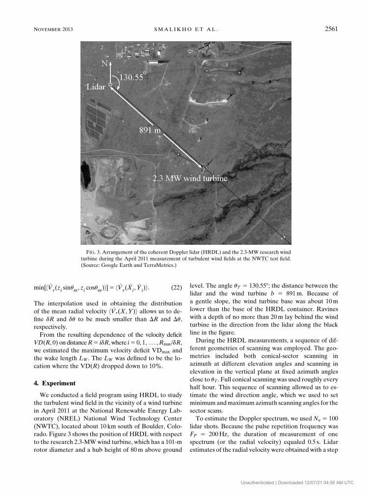
level. The angle uT 5 130.558; the distance between the

lidar and the wind turbine b 5 891m. Because of

a gentle slope, the wind turbine base was about 10m

lower than the base of the HRDL container. Ravines

with a depth of no more than 20m lay behind the wind

turbine in the direction from the lidar along the black

line in the figure.

During the HRDL measurements, a sequence of dif-

ferent geometries of scanning was employed. The geo-

metries included both conical-sector scanning in

azimuth at different elevation angles and scanning in

elevation in the vertical plane at fixed azimuth angles

close to uT . Full conical scanning was used roughly every

half hour. This sequence of scanning allowed us to es-

timate the wind direction angle, which we used to set

minimum andmaximum azimuth scanning angles for the

sector scans.

To estimate the Doppler spectrum, we used Na 5 100

lidar shots. Because the pulse repetition frequency was

FP 5 200Hz, the duration of measurement of one

spectrum (or the radial velocity) equaled 0.5 s. Lidar

estimates of the radial velocity were obtained with a step

FIG. 3. Arrangement of the coherent Doppler lidar (HRDL) and the 2.3-MW research wind

turbine during the April 2011 measurement of turbulent wind fields at the NWTC test field.

(Source: Google Earth and TerraMetrics.)



of DR 5 30m along the axis z0. The azimuth resolution

Du was 0.98 in the case of sector scanning. For full VAD

scanning, Du was 28 or 38.Examples of some realizations (without averaging and

interpolation) of two-dimensional distributions of

HRDL estimates of the radial velocity in the scanning

plane, including the distribution in the vertical plane

observed in these experiments, are reported in

Pichugina et al. (2011). The figures in Pichugina et al.

(2011) and Newsom and Banta (2004) for these distri-

butions show that, as the measurement range increases,

the number of bad estimates of the radial velocity also

increases because of the decrease in SNR. In addition,

estimates of the radial velocity are roughly zero at points

lying near the wind turbine as a result of the reflection of

the lidar pulse by the turbine blades (K€asler et al. 2010).

Therefore, to obtain the results presented below, we

used a specialized procedure, which allowed us to re-

place the velocity values at ‘‘zeroing’’ points with the

result of interpolation by neighboring points, at which

the radial velocity was estimated from aerosol back-

scatter unaffected by signal reflections off the turbine

blades. To minimize the influence of bad estimates on

the radial velocity at a long distance zi, we used the

procedure of filtering of good estimates through maxi-

mization of the functional

F(V)5 �N

n51

expf2[V2 Vr(zi, um;n)]2/(2s2)g (23)

[in place of Eq. (18)] when determining the 2D distri-

bution of the mean radial velocity. The parameter s was

taken as equal to 3m s21 in this case, that is, the mean

radial velocity was estimated as

max[F(V)]5F(hVr(zi, um)i) . (24)

Figure 4 illustrates the distribution of the radial ve-

locity in the scanning plane obtained from HRDL

measurements at elevation angles u5 28 (Fig. 4a) andu5 48 (Fig. 4b). For each of these two cases, we esti-

mated the wind direction angle uV using the technique

described in section 3. The white lines in Figs. 4a and 4c

are directed along the estimated wind direction angle

uV . Quantifications of the wind speeds along those lines

appear in Figs. 4b and 4d, and start from the turbine

FIG. 4. Distribution of the radial wind velocity in the scanning plane fX,Yg as obtained fromHRDLmeasurements at elevation angles

of (a) 28 and (c) 48 (c) from 2250 to 2300 LT 15 Apr 2011, and profiles of the wind velocity along lines 1 and 2 (starting from points marked

by white circles) at elevation angles of (b) 28 and (d) 48.



location (line 1) or the point A (line 2) at d5 1:2D 5120m (see section 3). The difference between the wind

velocities shown in the figure as curves 1 and 2 persists

for a longer downwind distance from the wind turbine at

u5 28 than at u5 48. At the same time, the maximum

deviation of velocities (consequently, the maximum

velocity deficit) took place at u5 48. This deviation was

related to the different position of scanning planes as

they intersected the turbine wake.

5. Results

For this case, sector scanning at elevation angles of 38–3.58was optimal for obtaining the information about the

wake structure. At a range of 890m (the location of the

turbine), heights of the laser beam relative to the wind

turbine base equaled 60m (20m below the turbine hub)

at u 5 38 and 67m (13m below the turbine hub) at u 53.58. At a range of 1890m, the heights of the laser beam

were 110m (u 5 38) and 128m (u 5 3.58) above the

turbine base elevation. Only these elevation angles (38and 3.58 alternately after each scan) were used for

HRDL measurements from 1920 LT 14 April 2011 to

1730 LT 15 April 2011. The duration of individual scan

sequences was, as a rule, 7min (57% of all cases) and

12min (41%). For each case, all data measured alter-

nately at elevation angles of 38 and 3.58 were used for

averaging [see Eqs. (23) and (24)]. We present the data

processing results of such measurements below.

Examples of the 2D distribution of the radial velocity

hVr(X,Y)i (Figs. 5a, 6a, and 7a), wind velocityUT(R)5U(R, 0) (curve 1) and UA(R) (curve 2) (Figs. 5b, 6b, and

7b), distribution of the wind-velocity deficit along the

wake axisVD(R, 0) (Figs. 5c, 6c, and 7c), and distributions

FIG. 5. (a) Distribution of the radial wind velocity in the scanning plane fX,Yg, as obtained from HRDL measurements at an

elevation angle of 38, from 1909 to 1916 LT 14 Apr 2011; (b) profiles of the wind velocity along white lines 1 and 2 starting from

points marked by white circles; (c) profiles of wind-velocity deficit VD(R, 0) along line 1, and (d) VD(R, x0) along the line per-

pendicular to lines 1 and 2 atR5 50m (curve 3,sT 5 51m), 150m (curve 4,sT 5 62m), 300m (curve 5,sT 5 74m), and 400m (curve 6,sT 578m).



of the wind-velocity deficit perpendicular to the wake

VD(R, x0) at different distances from the wind turbine

(Figs. 5d, 6d, and 7d) are shown. One can see a significant

difference in the wake length and velocity deficit for

the three time periods under consideration. We esti-

mated the transverse size of the wake sT , by fitting the

Gaussian model exp[2(x0/sT)2] to the measured value

of VD(R, x0)/VD(R, 0) by the least squares method.

Estimates of sT , which were obtained from the data of

Figs. 5d, 6d, and 7d, vary from 43 to 83m. Individual

estimates at different distances R are provided in the

captions of Figs. 5–7. In general sT increases with in-

creasing R.

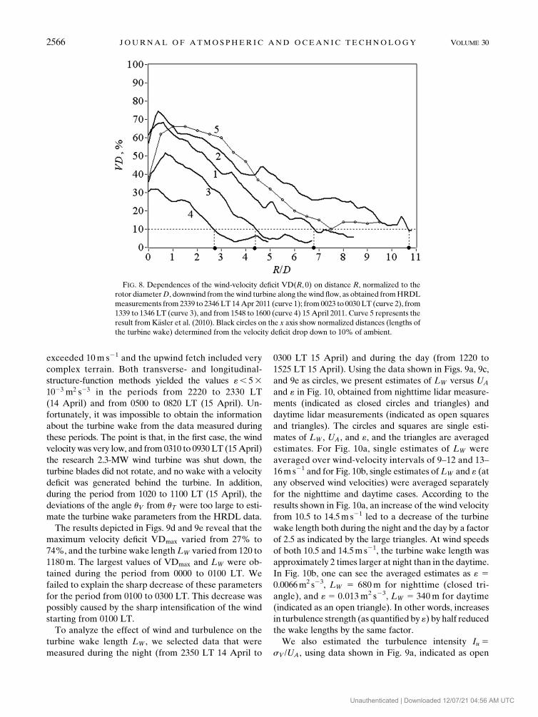
In Fig. 8, curves 1–4 show the dependency of velocity

deficit VD(R, 0) on the normalized distance on the lee-

ward side of the turbine, as obtained from HRDL

measurements. For comparison, curve 5 shows the ve-

locity deficit estimated from the data measured by

a CDL near Bremerhaven, Germany, during nighttime

at stable thermal stratification and very weak turbulence

(K€asler et al. 2010). It can be seen that curves 1 and 2,

obtained from nighttime HRDL data, are closest to

curve 5. The values of the normalized turbine wake

length LW /D are shown in the R/D axis as closed circles.

It can be seen that LW /D can change nearly tenfold for

different realizations. For the data shown in Fig. 8, the

maximum velocity deficit varied from 32% to 74%.

We used the data measured by full conical scanning

and an elevation angle of 108 (where there was no re-

flection of the signal by the wind turbine blades to

contaminate the measurement results) every half hour

for 24 h, starting from 1800 LT 14 April, to retrieve the

vertical profiles of the ambient wind velocity UA and

direction uV . The same lidar data were also used to re-

trieve vertical profiles of the turbulent parameters (such

as dissipation rate «, integral scaleLV , and wind-velocity

variance s2V) obtained using the transverse-structure-

function method described in section 2a. The resulting

FIG. 6. As in Fig. 5, but for 0018 to 0023 LT 15 Apr 2011and in (d) at R5 100m (curve 3, sT 5 60m), 300m (curve 4, sT 5 63m), 500m

(curve 5, sT 5 61m), and 1000m (curve 6, sT 5 76m).



temporal profiles of UA, uV , and « [indicated as the

turbulence energy dissipation rate (TEDR)] at h5 80m

(height of the wind turbine hub) are shown in Figs. 9a–c

as open squares connected with solid lines. Estimates of

the standard deviation sV [indicated as the standard

deviation of wind velocity (SDWV)] are shown in Fig. 9c

as closed squares connected by dashed lines. It can be

seen that during the period considered (from 1800 LT 14

April to 1800 LT 15 April), the wind velocity varied

from 2 to 18m s21. Most of the time, the wind velocity

exceeded 10m s21. In Fig. 9b, the obtained values of the

wind direction angle uV are shown by circles. These

circles aremostly concentrated near the dash-dotted line

that corresponds with the azimuth angle uT , between the

line passing through the lidar point in the direction to

the north and the line running through the lidar point

and the point of location of the turbine (see Fig. 3).

Typically, the deviations of the angle uV from uT did not

exceed 308 in absolute value, which allowed the turbine

wake information to be obtained from the lidar data and

main wake parameters to be monitored for almost the

entire period (when the turbine operated).

The processing procedures described earlier were used

to determine the ambientwind velocityUA (h5 80m) and

direction uV , themaximumvelocity deficit VDmax, and the

wake lengthLW , which are shown as circles in Figs. 9a, 9b,

9d, and 9e, from the lidar data measured by conical-sector

scanning across the wind turbine location. The same data

were also used to obtain the temporal profile of « at

a height of 80m, by using the longitudinal-structure-

functionmethod (see section 2b), which is shown as circles

in Fig. 9c. The results that are shown as circles and open

squares connected by solid lines in Figs. 9a–c are in a good

agreement most of the measurement time.

As seen in Fig. 9c, the experiment was mostly carried

out under conditions of strong («$ 1022 m2 s23) and

moderate (1023 m2 s23 # «, 1022 m2 s23) turbulence.

This was possibly related to the fact that wind speeds

FIG. 7. As in Fig. 5, but for 1518 to 1530 LT 15Apr 2011and in (d) atR5 50m (curve 3, sT 5 43m), 150m (curve 4, sT 5 65m), and 300m

(curve 5, sT 5 83m).



exceeded 10m s21 and the upwind fetch included very

complex terrain. Both transverse- and longitudinal-

structure-function methods yielded the values «, 531023 m2 s23 in the periods from 2220 to 2330 LT

(14 April) and from 0500 to 0820 LT (15 April). Un-

fortunately, it was impossible to obtain the information

about the turbine wake from the data measured during

these periods. The point is that, in the first case, the wind

velocity was very low, and from 0310 to 0930 LT (15April)

the research 2.3-MW wind turbine was shut down, the

turbine blades did not rotate, and no wake with a velocity

deficit was generated behind the turbine. In addition,

during the period from 1020 to 1100 LT (15 April), the

deviations of the angle uV from uT were too large to esti-

mate the turbine wake parameters from the HRDL data.

The results depicted in Figs. 9d and 9e reveal that the

maximum velocity deficit VDmax varied from 27% to

74%, and the turbine wake lengthLW varied from 120 to

1180m. The largest values of VDmax and LW were ob-

tained during the period from 0000 to 0100 LT. We

failed to explain the sharp decrease of these parameters

for the period from 0100 to 0300 LT. This decrease was

possibly caused by the sharp intensification of the wind

starting from 0100 LT.

To analyze the effect of wind and turbulence on the

turbine wake length LW , we selected data that were

measured during the night (from 2350 LT 14 April to

0300 LT 15 April) and during the day (from 1220 to

1525 LT 15 April). Using the data shown in Figs. 9a, 9c,

and 9e as circles, we present estimates of LW versus UA

and « in Fig. 10, obtained from nighttime lidar measure-

ments (indicated as closed circles and triangles) and

daytime lidar measurements (indicated as open squares

and triangles). The circles and squares are single esti-

mates of LW , UA, and «, and the triangles are averaged

estimates. For Fig. 10a, single estimates of LW were

averaged over wind-velocity intervals of 9–12 and 13–

16ms21 and for Fig. 10b, single estimates ofLW and « (at

any observed wind velocities) were averaged separately

for the nighttime and daytime cases. According to the

results shown in Fig. 10a, an increase of the wind velocity

from 10.5 to 14.5m s21 led to a decrease of the turbine

wake length both during the night and the day by a factor

of 2.5 as indicated by the large triangles. At wind speeds

of both 10.5 and 14.5m s21, the turbine wake length was

approximately 2 times larger at night than in the daytime.

In Fig. 10b, one can see the averaged estimates as « 50.0066m2 s23, LW 5 680m for nighttime (closed tri-

angle), and « 5 0.013m2 s23, LW 5 340m for daytime

(indicated as an open triangle). In other words, increases

in turbulence strength (as quantified by «) by half reduced

the wake lengths by the same factor.

We also estimated the turbulence intensity Iu 5sV /UA, using data shown in Fig. 9a, indicated as open

FIG. 8. Dependences of the wind-velocity deficit VD(R, 0) on distance R, normalized to the

rotor diameterD, downwind from thewind turbine along the wind flow, as obtained fromHRDL

measurements from 2339 to 2346 LT 14Apr 2011 (curve 1); from 0023 to 0030 LT (curve 2), from

1339 to 1346 LT (curve 3), and from 1548 to 1600 (curve 4) 15 April 2011. Curve 5 represents the

result fromK€asler et al. (2010). Black circles on the x axis show normalized distances (lengths of

the turbine wake) determined from the velocity deficit drop down to 10% of ambient.



squares, and in Fig. 9c, indicated as closed squares. After

averaging single estimates of Iu for periods 0000–0300

LT (when averaged wake lengthLW ’ 680m) and 1200–

1500 LT (when averaged wake length LW ’ 340m),

we obtained Iu 5 0.09 and Iu 5 0.15, respectively.

Therefore, when the turbulence intensity increased by

a factor of 0:15/0:9’ 1:7, the wake length reduced by

half.

FIG. 9. Diurnal profiles of the (a) ambient wind velocity, (b) wind direction, (c) TEDR and SDWV, (d) VDmax, and (e) turbine wake

lengthLW , all at a height of 80m as obtained from the data measured by HRDL using full conical scanning (open squares areUA, uV , and

«, and closed squares indicate sV). The « is estimated from the transverse structure function of the radial velocity (open squares) and from

the longitudinal structure function of the radial velocity calculated from HRDLmeasurements using sector scanning (circles). Estimates

shown as circles were obtained from HRDL sector scan measurements.



6. Conclusions

We investigated the turbulent wind field in the vicinity

of an operating wind turbine at the NWTC. In the field

experiment, our research team tested the method of

estimation of the turbulent energy dissipation rate from

the transverse structure function of the radial velocity

measured by a pulsed CDL using full 3608 conical

scanning. It was shown that this method was applicable

even in the case of one full conical scan. Methods were

also proposed for processing Doppler lidar–measured,

conical-sector scan data in the vicinity of a wind turbine

to estimate the wind speed and direction, the turbulent

energy dissipation rate, and parameters of the wake

generated by the wind turbine (maximum wind-velocity

deficit, and the longitudinal wake dimension).

FIG. 10. Turbine wake length versus (a) wind velocity and (b) turbulent energy dissipation

rate. Black circles and white squares are single estimates of UA, «, and LW from data

measured by HRDL at night (from 2350 LT Apr 14 to 0300 LT Apr 15) and during the day

(from 1220 to 1525 LT 15 Apr), respectively. Averaged estimates of LW that are within the

velocity intervals from 9–12m s21 and from 13–16m s21 are shown as black (nighttime) and

white (daytime) triangles in (a). The average estimate of LW and « over the indicated

measurement periods at night and during the day are shown as a black and white triangle,

respectively, in (b).



Using these approaches, we have determined the pa-

rameters of the turbulent wind field in the vicinity of the

wind turbine from measurements by the 2-mm pulsed

CDL on 14 and 15 April 2011, near Boulder, Colorado,

at the NWTC test field. In particular, it was found that

the wake behind the 2.3-MW research wind turbine,

with a rotor diameter of 101m and a hub height of 80m,

had the maximum velocity deficits of 27%–74% and

lengths from 120 to 1180m, depending on atmospheric

conditions. It has been shown that a doubling of the

turbulent energy dissipation rate (from .0066 to

0.013m2 s23) corresponded, on the average, to a halving

of the wake length (from 680 to 340m). Similarly, this

halving of the wake length is accompanied by an increase

in turbulence intensity by a factor of 1.7.

The study results indicate the high effectiveness of

using a pulsed 2-mm CDL to investigate turbulent wind

fields near wind power stations and wind farms, and

extend the range of problems addressed by atmospheric

laser sensing (Zakharov et al. 2010; Tsvyk et al. 2011;

Matvienko and Pogodaev 2012; Razenkov et al. 2012;

Banta et al. 2013). Future experiments similar to those

described in section 4 can yield the results necessary to

construct an empirical model of a turbine wake for

various atmospheric conditions.

Acknowledgments. We thank our colleagues from the

National Oceanic and Atmospheric Administration

(NOAA), including R. M. Hardesty, R.-J. Alvarez, S. P.

Sandberg, and A.M. Weickmann, and J. Mirocha from

the Lawrence Livermore National Laboratory for pre-

paring and conducting the experiment; John Brown from

NOAA for his help with weather forecasting; Andrew

Clifton from theNational Renewable Energy Laboratory

(NREL) for providing updates on tall-tower measure-

ments; Padriac Fowler and Paul Quelet for updates on

turbine operations; and Michael Stewart from NREL for

his help with security and safety issues. Funding for this

experiment was from the U.S. Department of Energy

Office of Energy Efficiency and Renewable EnergyWind

and Hydropower Technologies program. This work was

also supported by the Russian Foundation for Basic Re-

search (Project 10-05-9205) and theCivilianResearch and

Development Foundation (Project RUG1-2981-TO-10).

REFERENCES

Banakh, V. A., and I. N. Smalikho, 1997: Estimation of the tur-

bulence energy dissipation rate from the pulsed Doppler lidar

data. Atmos. Oceanic Opt., 10, 957–965.

——, ——, F. K€opp, and C. Werner, 1999: Measurements of tur-

bulent energy dissipation rate with a CW Doppler lidar in the

atmospheric boundary layer. J. Atmos. Oceanic Technol., 16,

1044–1061.

——, ——, Y. L. Pichugina, and W. A. Brewer, 2009: Represen-

tativeness of measurements of the turbulence energy dissipa-

tion rate by a scanning coherent Doppler lidar. Atmos.

Oceanic Opt., 22, 966–972.——, W. A. Brewer, Y. L. Pichugina, and I. N. Smalikho, 2010:

Wind velocity and direction measurement with a coherent

Doppler lidar under conditions of weak echo signal. Atmos.

Oceanic Opt., 23, 333–340.

Banta, R. M., R. K. Newsom, J. K. Lundquist, Y. L. Pichugina,

R. L. Coulter, and L. Mahrt, 2002: Nocturnal low-level jet

characteristics over Kansas during CASES-99. Bound.-Layer

Meteor., 105, 221–252.

——, Y. L. Pichugina, andW. A. Brewer, 2006: Turbulent velocity-

variance profiles in the stable boundary layer generated by

a nocturnal low-level jet. J. Atmos. Sci., 63, 2700–2719.

——,——, N. D. Kelley, R. M. Hardesty, andW. A. Brewer, 2013:

Wind energy meteorology: Insight into wind properties in the

turbine-rotor layer of the atmosphere from high-resolution

Doppler lidar. Bull. Amer. Meteor. Soc., 94, 883–902.

Barthelmie, R. J., L. Folkerts, F. T. Ormel, P. Sanderhoff, P. J.

Eecen, O. Stobbe, and N. M. Nielsen, 2003: Offshore wind

turbine wakesmeasured by sodar. J. Atmos. Oceanic Technol.,

20, 466–477.

——, ——, G. C. Larsen, K. Rados, S. C. Pryor, S. T. Frandsen,

B. Lange, and G. Schepers, 2006: Comparison of wake model

simulations with offshore wind turbine wake profiles mea-

sured by sodar. J. Atmos. Oceanic Technol., 23, 888–901.Bing€ol, F., J. Mann, and G. C. Larsen, 2010: Light detection and

ranging measurements of wake dynamics. Part I: One-

dimensional scanning. Wind Energy, 13, 51–61.

Browning, K. A., and R. Wexler, 1968: The determination of

kinematic properties of a wind field using Doppler radar.

J. Appl. Meteor., 7, 105–113.

Frehlich, R. G., and L. Cornman, 2002: Estimating spatial velocity

statistics with coherent Doppler lidar. J. Atmos. Oceanic

Technol., 19, 355–366.

——, S. M. Hannon, and S. W. Henderson, 1994: Performance

of a 2-mm coherent Doppler lidar for wind measurements.

J. Atmos. Oceanic Technol., 11, 1517–1528.

——, ——, and ——, 1998: Coherent Doppler lidar measurements

of wind field statistics. Bound.-Layer Meteor., 86, 223–256.——, Y. Meillier, M. L. Jensen, B. Balsley, and R. Sharman, 2006:

Measurements of boundary layer profiles in an urban envi-

ronment. J. Appl. Meteor. Climatol., 45, 821–837.Grund, C. J., R. M. Banta, J. L. George, J. N. Howell, M. J. Post,

R. A. Richter, and A. M. Weickman, 2001: High-resolution

Doppler lidar for boundary layer and cloud research. J. Atmos.

Oceanic Technol., 18, 376–393.

Hall, F. F., R. M. Huffaker, R. M. Hardesty, M. E. Jackson, T. R.

Lawrence, M. J. Post, R. A. Richter, and B. F. Weber, 1984:

Wind measurement accuracy of the NOAA pulsed infrared

Doppler lidar. Appl. Opt., 23, 2503–2506.

Hawley, J. G., R. Tang, S. W. Henderson, C. P. Hale, M. J.

Kavaya, and D. Moerder, 1993: Coherent launch-site at-

mospheric wind sounder: Theory and experiment. Appl.

Opt., 32, 4557–4567.

H€ogstr€om, U., D. N. Asimakopoulos, H. Kambezidis, C. G. Helmis,

and A. Smedman, 1987: A field study of the wake behind a

2MW wind turbine. Atmos. Environ., 22, 803–820.

K€asler, Y., S. Rahm, R. Simmet, and M. Kuhn, 2010: Wake mea-

surements of a multi-MW wind turbine with coherent long-

range pulsed Doppler wind lidar. J. Atmos. Oceanic Technol.,

27, 1529–1532.



Kelley, N. D., B. J. Jonkman, G. N. Scott, and Y. L. Pichugina,

2007: Comparing pulsed Doppler lidar with sodar and direct

measurements for wind assessment. Windpower Conf. and

Exhibition, Los Angeles, CA, American Wind Energy Asso-

ciation, NREL/CP-500-417.

K€opp, F., R. L. Schwiesow, and C. Werner, 1984: Remote mea-

surements of boundary layer wind profiles using a CW

Doppler lidar. J. Climate Appl. Meteor., 23, 148–154.——, S. Rahm, I. Smalikho, A. Dolfi, J.-P. Cariou, M. Harris, and

R. I. Young, 2005: Comparison of wake-vortex parameters

measured by pulsed and continuous-wave lidars. J. Aircr., 42,

916–923.

Magnusson, M., and A.-S. Smedman, 1996: Practical method to

estimate wind turbine wake characteristics from turbine data

and routine wind measurements. Wind Eng., 20, 73–92.Matvienko, G. G., and V. A. Pogodaev, 2012: Atmospheric and

ocean optics as uncompleted task of interaction of optical

radiation with a propagation medium. Atmos. Oceanic Opt.,

25, 5–10.Monin, A. S., and A. M. Yaglom, 1975: Mechanics of Turbulence.

Vol. 2, Statistical Fluid Mechanics, The MIT Press, 874 pp.

Newsom, R. K., and R. M. Banta, 2004: Assimilating coherent

Doppler lidar measurements into a model of the atmospheric

boundary layer. Part I:Algorithmdevelopment and sensitivity to

measurement error. J. Atmos. Oceanic Technol., 21, 1328–1345.

O’Connor, E. J., A. J. Illingworth, I. M. Brooks, C. D. Westbrook,

R. J. Hogan, F. Davies, and B. J. Brooks, 2010: A method for

estimating the kinetic energy dissipation rate from a vertically

pointing Doppler lidar, and independent evaluation from

balloon-borne in situ measurements. J. Atmos. Oceanic

Technol., 27, 1652–1664.

Pichugina, Y. L., and R. M. Banta, 2010: Stable boundary-layer

depth from high-resolution measurements of the mean wind

profile. J. Appl. Meteor. Climatol., 49, 20–35.——, S. C. Tucker, R. M. Banta, W. A. Brewer, N. D. Kelley, B. J.

Jonkman, and R. K. Newsom, 2008: Horizontal-velocity and

variance measurements in the stable boundary layer using

Doppler lidar: Sensitivity to averaging procedures. J. Atmos.

Oceanic Technol., 25, 1307–1327.

——, andCoauthors, 2011:Wind turbinewake study by theNOAA

high-resolutionDoppler lidar.Proc. 16th Coherent Laser Radar

Conf.,LongBeach,CA,Universities SpaceResearchAssociation,

4 pp. [Available online at http://sti.usra.edu/clrc2011/

presentations/Session%209/Summary%20Y%20Pichugina.

pdf.]

Rahm, S., and I. Smalikho, 2008: Aircraft wake vortex measure-

ment with airborne coherent Doppler lidar. J. Aircr., 45, 1148–

1155.

Razenkov, I. A., E. W. Eloranta, J. P. Hedrick, and J. P. Garcia,

2012: Arctic high spectral resolution lidar. Atmos. Oceanic

Opt., 25, 94–102.

Smalikho, I. N., 1997: Accuracy of the turbulent energy dissipation

rate estimation from the temporal spectrum of wind velocity

fluctuations. Atmos. Oceanic Opt., 10, 559–563.

——, 2003: Techniques of wind vector estimation from data mea-

sured with a scanning coherent Doppler lidar. J. Atmos.

Oceanic Technol., 20, 276–291.——, and V. A. Banakh, 2013: Accuracy of estimation of the tur-

bulent energy dissipation rate from wind measurements by

a pulsed coherent Doppler lidar at conical scanning by the

probing beam. Part I. Algorithm of data processing. Atmos.

Oceanic Opt., 26, 404–410.

——, F. K€opp, and S. Rahm, 2005: Measurement of atmospheric

turbulence by 2-mm Doppler lidar. J. Atmos. Oceanic Tech-

nol., 22, 1733–1747.

——, V. A. Banakh, Y. L. Pichugina, and W. A. Brewer, 2013:

Accuracy of estimation of the turbulent energy dissipation

rate from wind measurements by a pulsed coherent Doppler

lidar at conical scanning by the probing beam. Part II. Nu-

merical and atmospheric experiment. Atmos. Oceanic Opt.,

26, 411–416.Sonnenschein, C. M., and F. A. Horrigan, 1971: Signal-to-noise

relationships for coaxial systems that heterodyne backscatter

from the atmosphere. Appl. Opt., 10, 1600–1604.

Trujillo, J.-J., F. Bing€ol, G. C. Larsen, J. Mann, and M. K€uhn,2011: Light detection and ranging measurements of wake

dynamics. Part II: Two-dimensional scanning. Wind Energy,

14, 61–75.

Tsvyk, R. S., V. M. Sazanovich, and A. N. Shesternin, 2011:

Pointing of a laser beam based on laser beam aerosol back-

scattering. Modeling experiment. Atmos. Oceanic Opt., 24,

1056–1060.

Vermeer, L. J., J. N. Sorensen, and A. Crespo, 2003: Wind turbine

wake aerodynamics. Prog. Aerosp. Sci., 39, 467–510.

Vinnichenko, N. K., N. Z. Pinus, S. M. Shmeter, and G. N. Shur,

1973: Turbulence in the Free Atmosphere.Consultant’s Bureau,

263 pp.

Zakharov, V. M., O. K. Kostko, and V. U. Khattatov, 2010: Laser

applications for atmospheric research in CAO.Atmos. Oceanic

Opt., 23, 854–859.



http://sti.usra.edu/clrc2011/presentations/Session%209/Summary%20Y%20Pichugina.pdf



Date post:	07-Dec-2021
Category:	Documents
Upload:	others
View:	2 times
Download:	0 times

Lidar Investigation of Atmosphere Effect on a Wind Turbine ...

Documents