lil’ UCB : An Optimal Exploration Algorithm for Multi ... · JMLR: Workshop and Conference...

JMLR: Workshop and Conference Proceedings vol 35:1–17, 2014

lil’ UCB : An Optimal Exploration Algorithm for Multi-ArmedBandits ⇤

Kevin Jamieson [email protected] Malloy [email protected] Nowak [email protected] of Wisconsin

Sebastien Bubeck [email protected]

Princeton University

AbstractThe paper proposes a novel upper confidence bound (UCB) procedure for identifying the arm withthe largest mean in a multi-armed bandit game in the fixed confidence setting using a small numberof total samples. The procedure cannot be improved in the sense that the number of samplesrequired to identify the best arm is within a constant factor of a lower bound based on the law ofthe iterated logarithm (LIL). Inspired by the LIL, we construct our confidence bounds to explicitlyaccount for the infinite time horizon of the algorithm. In addition, by using a novel stopping timefor the algorithm we avoid a union bound over the arms that has been observed in other UCB-type algorithms. We prove that the algorithm is optimal up to constants and also show throughsimulations that it provides superior performance with respect to the state-of-the-art.Keywords: Multi-armed bandit, upper confidence bound (UCB), iterated logarithm

1. Introduction

This paper introduces a new algorithm for the best arm problem in the stochastic multi-armed bandit(MAB) setting. Consider a MAB with n arms, each with unknown mean payoff µ

1

, . . . , µn

in[0, 1]. A sample of the ith arm is an independent realization of a sub-Gaussian random variablewith mean µ

i

. In the fixed confidence setting, the goal of the best arm problem is to devise asampling procedure with a single input � that, regardless of the values of µ

1

, . . . , µn

, finds the armwith the largest mean with probability at least 1 � �. More precisely, best arm procedures mustsatisfy sup

µ

1

,...,µnP(bi 6= i⇤) �, where i⇤ is the best arm, bi an estimate of the best arm, and the

supremum is taken over all set of means such that there exists a unique best arm. In this sense,best arm procedures must automatically adjust sampling to ensure success when the mean of thebest and second best arms are arbitrarily close. Contrast this with the fixed budget setting where thetotal number of samples remains a constant and the confidence in which the best arm is identifiedwithin the given budget varies with the setting of the means. While the fixed budget and fixedconfidence settings are related (see Gabillon et al. (2012) for a discussion) this paper focuses on thefixed confidence setting only.

The best arm problem has a long history dating back to the ’50s with the work of Paulson(1964); Bechhofer (1958). In the fixed confidence setting, the last decade has seen a flurry of

⇤ Part of the research described here was carried out at the Simons Institute for the Theory of Computing. We aregrateful to the Simons Institute for providing a wonderful research environment.

c� 2014 K. Jamieson, M. Malloy, R. Nowak & S. Bubeck.

JAMIESON MALLOY NOWAK BUBECK

activity providing new upper and lower bounds. In 2002, the successive elimination procedure ofEven-Dar et al. (2002) was shown to find the best arm with order

Pi 6=i

⇤ ��2

i

log(n��2

i

) samples,where �

i

= µi

⇤ �µi

, coming within a logarithmic factor of the lower bound ofP

i 6=i

⇤ ��2

i

, shownin 2004 in Mannor and Tsitsiklis (2004). A similar bound was also obtained using a procedureknown as LUCB1 that was originally designed for finding the m-best arms (Kalyanakrishnan et al.,2012). Recently, Jamieson et al. (2013) proposed a procedure called PRISM which succeeds withP

i

�

�2

i

log log

⇣Pj

�

�2

j

⌘orP

i

�

�2

i

log

��

�2

i

�samples depending on the parameterization of

the algorithm, improving the result of Even-Dar et al. (2002) by at least a factor of log(n). The bestsample complexity result for the fixed confidence setting comes from a procedure similar to PRISM,called exponential-gap elimination (Karnin et al., 2013), which guarantees best arm identificationwith high probability using order

Pi

�

�2

i

log log�

�2

i

samples, coming within a doubly logarithmicfactor of the lower bound of Mannor and Tsitsiklis (2004). While the authors of Karnin et al. (2013)conjecture that the log log term cannot be avoided, it remained unclear as to whether the upperbound of Karnin et al. (2013) or the lower bound of Mannor and Tsitsiklis (2004) was loose.

The classic work of Farrell (1964) answers this question. It shows that the doubly logarith-mic factor is necessary, implying that order

Pi

�

�2

i

log log�

�2

i

samples are necessary and suf-ficient in the sense that no procedure can satisfy sup

�

1

,...,�nP(bi 6= i⇤) � and use fewer thanP

i

�

�2

i

log log�

�2

i

samples in expectation for all �1

, . . . ,�n

. The doubly logarithmic factor is aconsequence of the law of the iterated logarithm (LIL) (Darling and Robbins, 1985). The LIL statesthat if X

`

are i.i.d. sub-Gaussian random variables with E[X`

] = 0, E[X2

`

] = �2 and we defineSt

=

Pt

`=1

X`

then

lim sup

t!1Stp

2�

2

t log log(t)

= 1 and lim inf

t!1Stp

2�

2

t log log(t)

= �1

almost surely. Here is the basic intuition behind the lower bound. Consider the two-arm problemand let � be the difference between the means. In this case, it is reasonable to sample both armsequally and consider the sum of differences of the samples, which is a random walk with drift�. The deterministic drift crosses the LIL bound above when t� =

p2t log log t. Solving this

equation for t yields t ⇡ 2�

�2

log log�

�2. This intuition will be formalized in the next section.The LIL also motivates a novel approach to the best arm problem. Specifically, the LIL sug-

gests a natural scaling for confidence bounds on empirical means, and we follow this intuition todevelop a new algorithm for the best-arm problem. The algorithm is an Upper Confidence Bound(UCB) procedure (Auer et al., 2002) based on a finite sample version of the LIL. The new algo-rithm, called lil’UCB, is described in Figure 1. By explicitly accounting for the log log factor inthe confidence bound and using a novel stopping criterion, our analysis of lil’UCB avoids takingnaive union bounds over time, as encountered in some UCB algorithms (Kalyanakrishnan et al.,2012; Audibert et al., 2010), as well as the wasteful “doubling trick” often employed in algorithmsthat proceed in epochs, such as the PRISM and exponential-gap elimination procedures (Even-Daret al., 2002; Karnin et al., 2013; Jamieson et al., 2013). Also, in some analyses of best arm algo-rithms the upper confidence bounds of each arm are designed to hold with high probability for allarms uniformly, incurring a log(n) term in the confidence bound as a result of the necessary unionbound over the n arms (Even-Dar et al., 2002; Kalyanakrishnan et al., 2012; Audibert et al., 2010).However, our stopping time allows for a tighter analysis so that arms with larger gaps are allowedlarger confidence bounds than those arms with smaller gaps where higher confidence is required.Like exponential-gap elimination, lil’UCB is order optimal in terms of sample complexity.

2

LIL’ UCB : AN OPTIMAL EXPLORATION ALGORITHM FOR MULTI-ARMED BANDITS

It is easy to show that without the stopping condition (and with the right �) our algorithmachieves a cumulative regret of the same order as standard UCB. Thus for the expert it may besurprising that such an algorithm can achieve optimal sample complexity for the best arm identifi-cation problem given the lower bound of Bubeck et al. (2009). As it was empirically observed in thelatter paper there seems to be a transient regime, before this lower bound applies, where the perfor-mance in terms of best arm identification is excellent. In some sense the results in the present papercan be viewed as a formal proof of this transient regime: if stopped at the right time performance ofUCB for best arm identification is near-optimal (or even optimal for lil’UCB).

One of the main motivations for this work was to develop an algorithm that exhibits greatpractical performance in addition to optimal sample complexity. While the sample complexityof exponential-gap elimination is optimal up to constants, and PRISM up to small log log factors,the empirical performance of these methods is rather disappointing, even when compared to non-sequential sampling. Both PRISM and exponential-gap elimination employ median elimination(Even-Dar et al., 2002) as a subroutine. Median elimination is used to find an arm that is within" > 0 of the largest, and has sample complexity within a constant factor of optimal for this sub-problem. However, the constant factors tend to be quite large, and repeated applications of medianelimination within PRISM and exponential-gap elimination are extremely wasteful. On the con-trary, lil’UCB does not invoke wasteful subroutines. As we will show, in addition to having the besttheoretical sample complexities bounds known to date, lil’UCB also exhibits superior performancein practice with respect to state-of-the-art algorithms.

2. Lower Bound

Before introducing the lil’UCB algorithm, we show that the log log factor in the sample complexityis necessary for best-arm identification. It suffices to consider a two armed bandit problem with agap �. If a lower bound on the gap is unknown, then the log log factor is necessary, as shown bythe following result.

Theorem 1 Consider the best arm problem in the fixed confidence setting with n = 2, differ-ence between the two means �, and expected number of samples E

�

[T ]. Any procedure withsup

� 6=0

P(bi 6= i⇤) �, � 2 (0, 1/2), then has

lim sup

�!0

E�

[T ]

�

�2

log log�

�2

� 2� 4�.

Proof The proof follows readily from Theorem 1 of Farrell (1964) by considering a reduction of thebest arm problem with n = 2 in which the value of one arm is known. In this case, the only strategyavailable is to sample the other arm some number of times to determine if it is less than or greaterthan the known value. We have reduced the problem to the setting of (Farrell, 1964, Theorem 1),and stated it in Appendix A.

Theorem 1 implies that in the fixed confidence setting, no best arm procedure can have supP(bi 6=i⇤) � and use fewer than (2� 4�)

Pi

�

�2

i

log log�

�2

i

samples in expectation for all �i

.In brief, the result of Farrell follows by showing a generalized sequential probability ratio test,

which compares the running empirical mean of X after t samples against a series of thresholds,

3


is an optimal test. In the limit as t increases, if the thresholds are not at leastp(2/t) log log(t)

then the LIL implies the procedure will fail with probability approaching 1/2 for small values of�. Setting the thresholds to be just greater than

p(2/t) log log(t), in the limit, one can show the

expected number of samples must scale as ��2

log log�

�2. As the proof in Farrell (1964) is quiteinvolved, we provide a short argument for a slightly simpler result than above in Appendix A.

3. Procedure

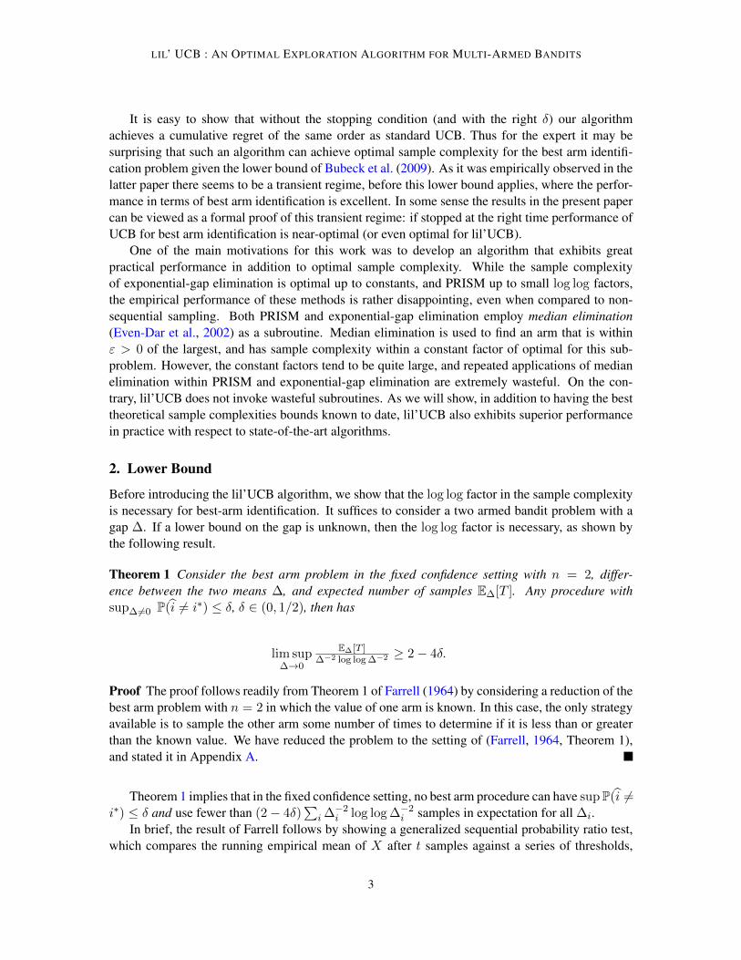
This section introduces lil’UCB. The procedure operates by sampling the arm with the largest upperconfidence bound; the confidence bounds are defined to account for the implications of the LIL.The procedure terminates when one of the arms has been sampled more than a constant timesthe number of samples collected from all other arms combined. Fig. 1 details the algorithm andTheorem 2 quantifies performance. In what follows, let X

i,s

, s = 1, 2, . . . denote independentsamples from arm i and let T

i

(t) denote the number of times arm i has been sampled up to timet. Define bµ

i,Ti(t):=

1

Ti(t)

PTi(t)

s=1

Xi,s

to be the empirical mean of the Ti

(t) samples from arm iup to time t. The algorithm of Fig. 1 assumes that the centered realizations of the ith arm aresub-Gaussian1 with known scale parameter �.

lil’ UCBinput: confidence � > 0, algorithm parameters ", �, � > 0

initialize: sample each of the n arms once, set Ti(t) = 1 for all i and set t = nwhile Ti(t) < 1 + �

Pj 6=i Tj(t) for all i

sample arm

It = argmax

i2{1,...,n}

8><

>:bµi,Ti(t) + (1 + �)(1 +

p")

vuut2�2

(1 + ") log⇣

log((1+")Ti(t))�

⌘

Ti(t)

9>=

>;.

set Ti(t+ 1) = Ti(t) + 1 if It = i, otherwise set Ti(t+ 1) = Ti(t).else stop and output argmaxi2{1,...,n} Ti(t)

Figure 1: The lil’ UCB algorithm.

Define

H1

=

X

i 6=i

⇤

1

�

2

i

and H3

=

X

i 6=i

⇤

log log

+

(1/�2

i

)

�

2

i

where log log

+

(x) = log log(x) if x � e, and 0 otherwise. Our main result is the following.

Theorem 2 For " 2 (0, 1), let c"

=

2+"

"

(1/ log(1 + "))1+" and fix � 2 (0, log(1 + ")/(ec"

)). Thenfor any � 2 (0, 3], there exists a constant � > 0 such that with probability at least 1�4

pc"

��4c"

�lil’ UCB stops after at most c

1

H1

log(1/�) + c3

H3

samples and outputs the optimal arm, wherec1

, c3

> 0 are known constants that depend only on ",�,�2.

1. A zero-mean random variable X is said to be sub-Gaussian with scale parameter � if for all t 2 R we haveE[exp{tX}] exp{�2t2/2}. If a X b almost surely than it suffices to take �2

= (b� a)2/4.

4


Note that the algorithm obtains the optimal query complexity of H1

log(1/�) +H3

up to con-stant factors. We remark that the theorem holds with any value of � satisfying (7). Inspection of (7)

shows that as � ! 0 we can let � tend to⇣2+�

�

⌘2

. We point out that the sample complexity boundin the theorem can be optimized by choosing " and �. For a setting of these parameters in a way that

is more or less faithful to the theory, we recommend taking " = 0.01, � = 1, and � =

⇣2+�

�

⌘2

. Forimproved performance in practice, we recommend applying footnote 2 and setting " = 0, � = 0.5,� = 1 + 10/n and � 2 (0, 1), which do not meet the requirements of the theorem, but work verywell in our experiments presented later. We prove the theorem via two lemmas, one for the totalnumber of samples taken from the suboptimal arms and one for the correctness of the algorithm. Inthe lemmas we give precise constants.

4. Proof of Theorem 2

Before stating the two main lemmas that imply the result, we first present a finite form of the lawof iterated logarithm. This finite LIL bound is necessary for our analysis and may also prove usefulfor other applications.

Lemma 3 Let X1

, X2

, . . . be i.i.d. centered sub-Gaussian random variables with scale param-eter �. For any " 2 (0, 1) and � 2 (0, log(1 + ")/e)2 one has with probability at least 1 �2+"

"

⇣�

log(1+")

⌘1+"

for all t � 1,

tX

s=1

Xs

(1 +

p")

s

2�2(1 + ")t log

✓log((1 + ")t)

�

◆.

Proof We denote St

=

Pt

s=1

Xs

, and (x) =r2�2x log

⇣log(x)

�

⌘. We also define by induction

the sequence of integers (uk

) as follows: u0

= 1, uk+1

= d(1 + ")uk

e.Step 1: Control of S

uk , k � 1. The following inequalities hold true thanks to an union boundtogether with Chernoff’s bound, the fact that u

k

� (1+ ")k, and a simple sum-integral comparison:

P�9k � 1 : S

uk �p1 + " (u

k

)

�

1X

k=1

exp

⇣�(1 + ") log

⇣log(uk)

�

⌘⌘

1X

k=1

⇣�

k log(1+")

⌘1+"

�1 +

1

"

� ⇣�

log(1+")

⌘1+"

.

Step 2: Control of St

, t 2 (uk

, uk+1

). Adopting the notation [n] = {1, . . . , n}, recall that Hoeffd-ing’s maximal inequality3 states that for any m � 1 and x > 0 one has

P(9 t 2 [m] s.t. St

� x) exp

⇣� x

2

2�

2

m

⌘.

2. Note � is restricted to guarantee that log( log((1+")t)� ) is well defined. This makes the analysis cleaner but in practice

one can allow the full range of � by using log(

log((1+")t+2)

� ) instead and obtain the same theoretical guarantees.3. It is an easy exercise to verify that Azuma-Hoeffding holds for martingale differences with sub-Gaussian increments,

which implies Hoeffding’s maximal inequality for sub-Gaussian distributions.

5


Thus the following inequalities hold true (by using trivial manipulations on the sequence (uk

)):

P�9 t 2 {u

k

+ 1, . . . , uk+1

� 1} : St

� Suk �

p" (u

k+1

)

�

= P�9 t 2 [u

k+1

� uk

� 1] : St

�p" (u

k+1

)

� exp

⇣�" uk+1

uk+1

�uk�1

log

⇣log(uk+1

)

�

⌘⌘

exp

⇣�(1 + ") log

⇣log(uk+1

)

�

⌘⌘⇣

�

(k+1) log(1+")

⌘1+"

.

Step 3: By putting together the results of Step 1 and Step 2 we obtain that with probability at least

1� 2+"

"

⇣�

log(1+")

⌘1+"

, one has for any k � 0 and any t 2 {uk

+ 1, . . . , uk+1

},

St

= St

� Suk + S

uk

p" (u

k+1

) +

p1 + " (u

k

)

p" ((1 + ")t) +

p1 + " (t)

(1 +

p") ((1 + ")t),

which concludes the proof.

Without loss of generality we assume that µ1

> µ2

� . . . � µn

. To shorten notation we denote

U(t,!) = (1 +

p")

r2�

2

(1+")

t

log

⇣log((1+")t)

!

⌘.

The following events will be useful in the analysis:

Ei

(!) = {8t � 1, |bµi,t

� µi

| U(t,!)}

where bµi,t

=

1

t

Pt

j=1

xi,j

. Note that Lemma 3 shows P(Ei

(!)c) = O(!). The following trivialinequalities will also be useful (the second one is derived from the first inequality and the fact thatx+a

x+b

a

b

for a � b, x � 0). For t � 1, " 2 (0, 1), c > 0, 0 < ! 1,

1

tlog

✓log((1 + ")t)

!

◆� c ) t 1

clog

✓2 log((1 + ")/(c!))

!

◆, (1)

and for t � 1, s � 3, " 2 (0, 1), c 2 (0, 1], 0 < ! � e�e,

1

tlog

✓log((1 + ")t)

!

◆� c

slog

✓log((1 + ")s)

�

◆and ! � ) t s

c

log

�2 log

�1

c!

�/!�

log(1/�). (2)

Lemma 4 Let �, ", � be set as in Theorem 2 and let � = 2(2 + �)2(1 +

p")2�2(1 + ") and

c"

=

2+"

"

⇣1

log(1+")

⌘1+"

. Then we have with probability at least 1� 2c"

� and any t � 1,

nX

i=2

Ti

(t) n+ 5�H1

log(e/�) +nX

i=2

�log(2max{1, log(�(1 + ")/�2

i

/�)})�

2

i

.

6


The proof relies crucially on the fact that the realizations from each arm are independent of eachother. This means that if we condition on the event that the realizations from the optimal arm arewell-behaved, it is shown that the number of times the ith suboptimal arm is pulled is an independentsub-exponential random variable with mean on the order of ��2

i

log(log(�

�2

i

)/�). We then apply astandard tail bound to the sum of independent sub-exponential random variables to obtain the result.Proof We decompose the proof in two steps.Step 1. Let i > 1. Assuming that E

1

(�) and Ei

(!) hold true and that It

= i one has

µi

+U(Ti

(t),!)+(1+�)U(Ti

(t), �) � bµi,Ti(t)

+(1+�)U(Ti

(t), �) � bµ1,T

1

(t)

+(1+�)U(T1

(t), �) � µ1

,

which implies (2 + �)U(Ti

(t),min(!, �)) � �

i

. If � = 2(2 + �)2(1 +p")2�2(1 + ") then using

(1) with c =�

2

i�

one obtains that if E1

(�) and Ei

(!) hold true and It

= i then

Ti

(t) �

�

2

i

log

✓2 log(�(1 + ")/�2

i

/min(!, �))

min(!, �)

◆

⌧i

+

�

�

2

i

log

✓log(e/!)

!

◆ ⌧

i

+

2�

�

2

i

log

✓1

!

◆,

where ⌧i

=

�

�

2

ilog

⇣2max{1,log(�(1+")/�

2

i /�)}�

⌘.

Since Ti

(t) only increases when i is played the above argument shows that the following in-equality is true for any time t � 1:

Ti

(t)1{E1

(�) \ Ei

(!)} 1 + ⌧i

+

2�

�

2

i

log

✓1

!

◆. (3)

Step 2. We define the following random variable:

⌦

i

= max{! � 0 : Ei

(!) holds true}.

Note that ⌦

i

is well-defined and by Lemma 3 it holds that P(⌦i

< !) c"

! where c"

=

2+"

"

⇣1

log(1+")

⌘1+"

. Furthermore one can rewrite (3) as

Ti

(t)1{E1

(�)} 1 + ⌧i

+

2�

�

2

i

log

✓1

⌦

i

◆. (4)

We use this equation as follows:

P

nX

i=2

Ti

(t) > x+

nX

i=2

(⌧i

+ 1)

! c

"

� + P

nX

i=2

Ti

(t) > x+

nX

i=2

(⌧i

+ 1)

�� E1(�)!

c"

� + P

nX

i=2

2�

�

2

i

log

✓1

⌦

i

◆> x

!. (5)

Let Zi

=

2�

�

2

ilog

⇣c

�1

"⌦i

⌘, i 2 [n] \ 1. Observe that these are independent random variables and since

P(⌦i

< !) c"

! it holds that P(Zi

> x) exp(�x/ai

) with ai

= 2�/�2

i

. Using standard

7


techniques to bound the sum of sub-exponential random variables one directly obtains that

P

nX

i=2

(Zi

� ai

) � z

! exp

✓�min

⇢z2

4kak22

,z

4kak1

�◆ exp

✓�min

⇢z2

4kak21

,z

4kak1

�◆.

(6)Putting together (5) and (6) with z = 4kak

1

log(1/(c"

�)), x = z + ||a||1

log(ec"

) one obtains

P

nX

i=2

Ti

(t) >

nX

i=2

✓4� log(e/�)

�

2

i

+ ⌧i

+ 1

◆! 2c

"

�,

which concludes the proof.

Lemma 5 Let �, ", � be set as in Theorem 2 and let c"

=

2+"

"

⇣1

log(1+")

⌘1+"

. If

� �1+

log

✓2 log

✓(

2+�� )

2

/�

◆◆

log(1/�)

1�(c"�)�p

(c"�)1/4

log(1/(c"�))

⇣2+�

�

⌘2

, (7)

then for all i = 2, . . . , n and t = 1, 2, . . . , we have Ti

(t) < 1 + �P

j 6=i

Tj

(t) with probability atleast 1� 2c

"

� + 4

pc"

�.

Note that the right hand side of (7) can be bound by a universal constant for all allowable � whichleads to the simplified statement of Theorem 2. Moreover, for any ⌫ > 0 there exists a sufficiently

small � 2 (0, 1) such that the right hand side of (7) is less than or equal to (1 + ⌫)⇣2+�

�

⌘2

.Essentially, the proof relies on the fact that given any two arms j < i (i.e. µ

j

� µi

), Ti

(t)cannot be larger than a constant times T

j

(t) with probability at least 1� �. Considering this fact, itis reasonable to suppose that the probability that T

i

(t) is larger than a constant timesP

i�1

j=1

Tj

(T ) isdecreasing exponentially fast in i. Consequently, our stopping condition is not based on a uniformconfidence bound for all arms. Rather, it is based on confidence bounds that grow in size as the armindex i increases.Proof We decompose the proof in two steps.Step 1. Let i > j. Assuming that E

i

(!) and Ej

(�) hold true and that It

= i one has

µi

+ U(Ti

(t),!) + (1 + �)U(Ti

(t), �) � bµi,Ti(t)

+ (1 + �)U(Ti

(t), �)

� bµj,Tj(t)

+ (1 + �)U(Tj

(t), �) � µj

+ �U(Tj

(t), �),

which implies (2 + �)U(Ti

(t),min(!, �)) � �U(Tj

(t), �). Thus using (2) with c =

⇣�

2+�

⌘2

oneobtains that if E

i

(!) and Ej

(�) hold true and It

= i then

Ti

(t) ⇣2+�

�

⌘2

log

✓2 log

✓⇣2+��

⌘2

/min(!,�)

◆/min(!,�)

◆

log(1/�)

Tj

(t).

Similarly to Step 1 in the proof of Lemma 4 we use the fact that Ti

(t) only increases when It

isplayed and the above argument to obtain the following inequality for any time t � 1:

(Ti

(t)� 1)1{Ei

(!) \ Ej

(�)} ⇣2+�

�

⌘2

log

✓2 log

✓⇣2+��

⌘2

/min(!,�)

◆/min(!,�)

◆

log(1/�)

Tj

(t). (8)

8


Step 2. Using (8) with ! = �i�1 we see that

1{Ei

(�i�1

)} 1

i� 1

i�1X

j=1

1{Ej

(�)} > 1� ↵ ) (1� ↵)(Ti

(t)� 1) X

j 6=i

Tj

(t)

where =

⇣2+�

�

⌘2

✓1+

log

✓2 log

✓⇣2+��

⌘2

/�

◆◆

log(1/�)

◆. This implies the following, using that P(E

i

(!)) �1� c

"

!,

P

0

@9 (i, t) 2 {2, . . . , n}⇥ {1, . . . } : (1� ↵)(Ti

(t)� 1) � X

j 6=i

Tj

(t)

1

A

P

0

@9 i 2 {2, . . . , n} : 1{Ei

(�i�1

)} 1

i� 1

i�1X

j=1

1{Ej

(�)} 1� ↵

1

A

nX

i=2

P(Ei

(�i�1

) does not hold) +nX

i=2

P

0

@ 1

i� 1

i�1X

j=1

1{Ej

(�)} 1� c"

� � (↵� c"

�)

1

A .

Let �0 = c"

�. Note that by a simple Hoeffding’s inequality and a union bound one has

P

0

@ 1

i� 1

i�1X

j=1

1{Ej

(�)} 1� �0 � (↵� �0)

1

A min((i� 1)�0, exp(�2(i� 1)(↵� �0)2),

and thus if we define j⇤ = d�0�1/4/2e we obtain with the above calculations

P

0

@9 (i, t) 2 {2, . . . , n}⇥ {1, . . . } :

⇣1� �0 �

p�01/4 log(1/�0)

⌘(T

i

(t)� 1) � X

j 6=i

Tj

(t)

1

A

nX

i=2

⇣�0i�1

+min

⇣(i� 1)�0, e�2(i�1)�

01/4log

(

1

�0 )⌘⌘

�0

1� �0+ �0j2⇤ +

e�2j⇤�01/4

log

(

1

�0 )

1� e�2�

01/4log

(

1

�0 )

�0

1� �0+

9

4

�01/2 + 3

2

�03/4 2c"

� + 4

pc"

�.

Treating ", �2 and factors of log log(�) as constants, Lemma 4 says that the total number of timesthe suboptimal arms are sampled does not exceed (� + 2)

2

(c1

H1

log(1/�) + c3

H3

). Lemma 5

states that only the optimal arm will meet the stopping condition with � = c�

⇣2+�

�

⌘2

for some c�

constant defined in the lemma. Combining these results, we observe that the total number of times

all the arms are sampled does not exceed (� + 2)

2

(c1

H1

log(1/�) + c3

H3

)

✓1 + c

�

⇣2+�

�

⌘2

◆,

completing the proof of the theorem. We also observe using the approximation c�

= 1, the optimalchoice of � ⇡ 1.66.

9


5. Implementation and Simulations

In this section we investigate how the state of the art methods for solving the best arm problembehave in practice. Before describing each of the algorithms in the comparison, we briefly describea LIL-based stopping criterion that can be applied to any of the algorithms.

LIL Stopping (LS) : For any algorithm and i 2 [n], after the t-th time we have that the i-tharm has been sampled T

i

(t) times and accumulated a mean bµi,Ti(t)

. We can apply Lemma 3

(with a union bound) so that with probability at least 1� 2+"

"

⇣�

log(1+")

⌘1+"

��bµi,Ti(t)

� µi

�� Bi,Ti(t)

:= (1 +

p")

r2�

2

(1+") log

⇣2 log((1+")Ti(t)+2)

�/n

⌘

Ti(t)(9)

for all t � 1 and all i 2 [n]. We may then conclude that if bi := argmax

i2[n] bµi,Ti(t)and

bµbi,Tbi(t)

�Bbi,Tbi(t)

� bµj,Tj(t)

+Bj,Tj(t)

8j 6= bi then with high probability we have thatbi = i⇤.

The LIL stopping condition is somewhat naive but often quite effective in practice for smaller sizeproblems when log(n) is negligible. To implement the strategy for any algorithm with fixed confi-dence ⌫, simply run the algorithm with ⌫/2 in place of ⌫ and assign the other ⌫/2 confidence to theLIL stopping criterion. Note that to for the LIL bound to hold with probability at least 1 � ⌫, one

should use � = log(1 + ")⇣

⌫"

2+"

⌘1/(1+")

. The algorithms compared were:

• Nonadaptive + LS : Draw a random permutation of [n] and sample the arms in an orderdefined by cycling through the permutation until the LIL stopping criterion is met.

• Exponential-Gap Elimination (+LS) (Karnin et al., 2013) : This procedure proceeds in stageswhere at each stage, median elimination (Even-Dar et al., 2002) is used to find an "-optimalarm whose mean is guaranteed (with large probability) to be within a specified " > 0 of themean of the best arm, and then arms are discarded if their empirical mean is sufficiently belowthe empirical mean of the "-optimal arm. The algorithm terminates when there is only onearm that has not yet been discarded (or when the LIL stopping criterion is met).

• Successive Elimination (Even-Dar et al., 2002) : This procedure proceeds in the same spirit asExponential-Gap Elimination except the "-optimal arm is equal tobi := argmax

i2[n] bµi,Ti(t).

• lil’UCB (+LS) : The procedure of Figure 1 is run with " = 0.01, � = 1, � = (2+�)2/�2 = 9,

and � = (

p1+⌫(/2)�1)

2

4c"for input confidence ⌫. The algorithm terminates according to Fig. 1

(or when the LIL stopping criterion is met). Note that � is defined as prescribed by Theorem 2but we approximate the leading constant in (7) by 1 to define �.

• lil’UCB Heuristic : The procedure of Figure 1 is run with " = 0, � = 1/2, � = 1 + 10/n,and � = ⌫/5 for input confidence ⌫. These parameter settings do not satisfy the conditions ofTheorem 2, and thus there is no guarantee that this algorithm will find the best arm.

• LUCB1 (+ LS) (Kalyanakrishnan et al., 2012) : This procedure pulls two arms at each time:the arm with the highest empirical mean and the arm with the highest upper confidence boundamong the remaining arms. The upper confidence bound was of the form prescribed in thesimulations section of Kaufmann and Kalyanakrishnan (2013) and is guaranteed to return thearm with the highest mean with confidence 1� �.

10


We did not compare to PRISM of Jamieson et al. (2013) because the algorithm and its empirical per-formance are very similar to Exponential-Gap Elimination so its inclusion in the comparison wouldprovide very little added value. We remark that the first three algorithms require O(1) amortizedcomputation per time step, the lil’UCB algorithms require O(log(n)) computation per time stepusing smart data structures4, and LUCB1 requires O(n) computation per time step. LUCB1 wasnot run on all problem sizes due to poor computational scaling with respect to the problem size.

Three problem scenarios were considered over a variety problem sizes (number of arms). The“1-sparse” scenario sets µ

1

= 1/2 and µi

= 0 for all i = 2, . . . , n resulting in a hardness ofH

1

= 4n. The “↵ = 0.3” and “↵ = 0.6” scenarios consider n + 1 arms with µ0

= 1 andµi

= 1 � (i/n)↵ for all i = 1, . . . , n with respective hardnesses of H1

⇡ 3/2n and H1

⇡ 6n1.2.That is, the ↵ = 0.3 case should be about as hard as the sparse case with increasing problem sizewhile the ↵ = 0.6 is considerably more challenging and grows super linearly with the problem size.See Jamieson et al. (2013) for an in-depth study of the ↵ parameterization. All experiments wererun with input confidence � = 0.1. All realizations of the arms were Gaussian random variableswith mean µ

i

and variance 1/45.Each algorithm terminates at some finite time with high probability so we first consider the

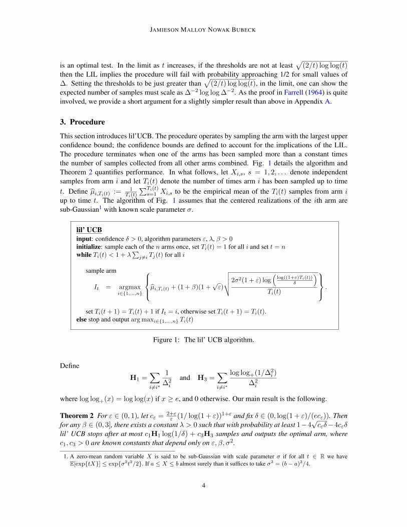
relative stopping times of each of the algorithms in Figure 2. Each algorithm was run on eachproblem scenario and problem size, repeated 50 times. The first observation is that Exponential-Gap Elimination (+LS) appears to barely perform better than nonadaptive sampling with the LILstopping criterion. This confirms our suspicion that the constants in median elimination are justtoo large to make this algorithm practically relevant. While the LIL stopping criterion seems tohave measurably improved the lil’UCB algorithm, it had no impact on the lil’UCB Heuristic variant(not plotted). While lil’UCB Heuristic has no theoretical guarantees of outputting the best arm, weremark that over the course of all of our tens of thousands of experiments, the algorithm never failedto terminate with the best arm. The LUCB algorithm, despite having worse theoretical guaranteesthan the lil’UCB algorithm, performs surprisingly well. We conjecture that this is because UCBstyle algorithms tend to lean towards exploiting the top arm versus focusing on increasing the gapbetween the top two arms, which is the goal of LUCB.

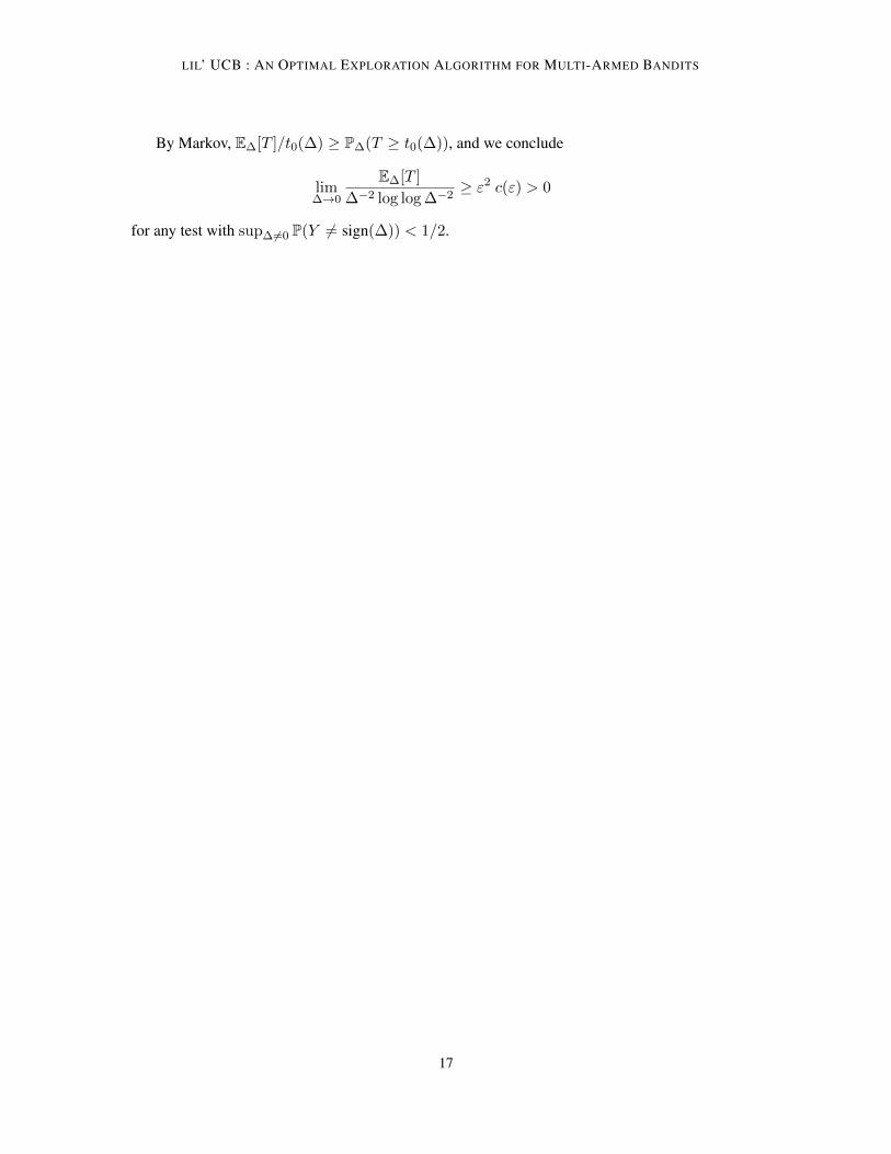
In reality, one cannot always wait for an algorithm to run until it terminates on its own so we nowexplore how the algorithms perform if the algorithm must output an arm at every time step beforetermination (this is similar to the setting studied in Bubeck et al. (2009)). For each algorithm, at eachtime we output the arm with the highest empirical mean. Clearly, the probability that a sub-optimalarm is output by any algorithm should very close to 1 in the beginning but then eventually decrease toat least the desired input confidence, and likely, to zero. Figure 3 shows the “anytime” performanceof the algorithms for the three scenarios and unlike the empirical stopping times of the algorithms,we now observe large differences between the algorithms. Each experiment was repeated 5000times. Again we see essentially no difference between nonadaptive sampling and the exponential-gap procedure. While in the stopping time plots of Figure 2 the successive elimination appearscompetitive with the UCB algorithms, we observe in Figure 3 that the UCB algorithms are collecting

4. The sufficient statistic for lil’UCB to decide which arm to sample depends only on bµi,Ti(t) and Ti(t) which onlychanges for an arm if that particular arm is pulled. Thus, it suffices to maintain an ordered list of the upper confidencebounds in which deleting, updating, and reinserting the arm requires just O(log(n)) computation. Contrast this witha UCB procedure in which the upper confidence bounds depend explicitly on t so that the sufficient statistics forpulling the next arm changes for all arms after each pull, requiring ⌦(n) computation per time step.

5. The variance was chosen such that the analyses of algorithms that assumed realizations were in [0, 1] and usedHoeffding’s inequality were still valid using sub-Gaussian tail bounds with scale parameter 1/2.

11


1-sparse, H1

= 4n ↵ = 0.3, H1

⇡ 3

2

n ↵ = 0.6, H1

⇡ 6n1.2

Figure 2: Stopping times of the algorithms for three scenarios for a variety of problem sizes. Theproblem scenarios from left to right are the 1-sparse problem (µ

1

= 0.5, µi

= 0 8i > 1),↵ = 0.3 (µ

i

= 1� (i/n)↵, i = 0, 1, . . . , n), and ↵ = 0.6.

sufficient information to output the best arm at least twice as fast as successive elimination. Thistells us that the stopping conditions for the UCB algorithms are still too conservative in practicewhich motivates the use of the lil’UCB Heuristic algorithm which appears to perform very stronglyacross all metrics. The LUCB algorithm again performs strongly here suggesting that LUCB-stylealgorithms are very well-suited for exploration tasks.

6. Discussion

This paper proposed a new procedure for identifying the best arm in a multi-armed bandit problemin the fixed confidence setting, a problem of pure exploration. However, there are some scenarioswhere one wishes to balance exploration with exploitation and the metric of interest is the cumu-lative regret. We remark that the techniques developed here can be easily extended to show thatthe lil’UCB algorithm obtains bounded regret with high probability, improving upon the result ofAbbasi-Yadkori et al. (2011).

In this work we proved upper and lower bounds over the class of distributions with boundedmeans and sub-Guassian realizations and presented our results just in terms of the difference be-tween the means of the arms. In contrast to just considering the means of the distributions, Kauf-mann and Kalyanakrishnan (2013) studied the Chernoff information between distributions, a quan-tity related to the KL divergence, that is sharper and can result in improved rates in identifying thebest arm in theory and practice (for instance if the realizations from the arms have very differentvariances). Pursuing methods that exploit distributional characteristics beyond the mean is a gooddirection for future work.

Finally, an obvious extension of this work is to consider finding the top-m arms instead ofjust the best arm. This idea has been explored in both the fixed confidence setting Kaufmann andKalyanakrishnan (2013) and the fixed budget setting Bubeck et al. (2012) but we believe both ofthese sample complexity results to be suboptimal. It may be possible to adapt the approach devel-oped in this paper to find the top-m arms and obtain gains in theory and practice.

12


1-sparse, H1

= 4n ↵ = 0.3, H1

⇡ 3

2

n ↵ = 0.6, H1

⇡ 6n1.2

n=

10

n=

100

n=

1000

n=

10000

Figure 3: At every time, each algorithm outputs an arm ˆi that has the highest empirical mean. TheP(ˆi 6= i⇤) is plotted with respect to the total number of pulls by the algorithm. The prob-lem sizes (number of arms) increase from top to bottom. The problem scenarios from leftto right are the 1-sparse problem (µ

1

= 0.5, µi

= 0 8i > 1) , ↵ = 0.3 (µi

= 1� (i/n)↵,i = 0, 1, . . . , n), and ↵ = 0.6. The arrows indicate the stopping times (if not shown,those algorithms did not terminate within the time window shown). Note that LUCB1is not plotted for n = 10000 due to computational constraints (see text for explanation).Also note that in some plots it is difficult to distinguish between the nonadaptive samplingprocedure, the exponential-gap algorithm, and successive elimination due to the curvesbeing on top of each other.

13


References

Yasin Abbasi-Yadkori, Csaba Szepesvari, and David Tax. Improved algorithms for linear stochasticbandits. In Advances in Neural Information Processing Systems, pages 2312–2320, 2011.

Jean-Yves Audibert, Sebastien Bubeck, and Remi Munos. Best arm identification in multi-armedbandits. COLT 2010-Proceedings, 2010.

Peter Auer, Nicolo Cesa-Bianchi, and Paul Fischer. Finite-time analysis of the multiarmed banditproblem. Machine learning, 47(2-3):235–256, 2002.

Robert E Bechhofer. A sequential multiple-decision procedure for selecting the best one of severalnormal populations with a common unknown variance, and its use with various experimentaldesigns. Biometrics, 14(3):408–429, 1958.

S. Bubeck, R. Munos, and G. Stoltz. Pure exploration in multi-armed bandits problems. In Pro-ceedings of the 20th International Conference on Algorithmic Learning Theory (ALT), 2009.

Sebastien Bubeck, Tengyao Wang, and Nitin Viswanathan. Multiple identifications in multi-armedbandits. arXiv preprint arXiv:1205.3181, 2012.

DA Darling and Herbert Robbins. Iterated logarithm inequalities. In Herbert Robbins SelectedPapers, pages 254–258. Springer, 1985.

Eyal Even-Dar, Shie Mannor, and Yishay Mansour. PAC bounds for multi-armed bandit and markovdecision processes. In Computational Learning Theory, pages 255–270. Springer, 2002.

R. H. Farrell. Asymptotic behavior of expected sample size in certain one sided tests. The Annalsof Mathematical Statistics, 35(1):pp. 36–72, 1964. ISSN 00034851.

Victor Gabillon, Mohammad Ghavamzadeh, Alessandro Lazaric, and Team SequeL. Best arm iden-tification: A unified approach to fixed budget and fixed confidence. In NIPS, pages 3221–3229,2012.

Kevin Jamieson, Matthew Malloy, Robert Nowak, and Sebastien Bubeck. On finding the largestmean among many. arXiv preprint arXiv:1306.3917, 2013.

Shivaram Kalyanakrishnan, Ambuj Tewari, Peter Auer, and Peter Stone. PAC subset selection instochastic multi-armed bandits. In Proceedings of the 29th International Conference on MachineLearning (ICML-12), pages 655–662, 2012.

Zohar Karnin, Tomer Koren, and Oren Somekh. Almost optimal exploration in multi-armed bandits.In Proceedings of the 30th International Conference on Machine Learning, 2013.

Emilie Kaufmann and Shivaram Kalyanakrishnan. Information complexity in bandit subset selec-tion. COLT, 2013.

Shie Mannor and John N Tsitsiklis. The sample complexity of exploration in the multi-armed banditproblem. The Journal of Machine Learning Research, 5:623–648, 2004.

Edward Paulson. A sequential procedure for selecting the population with the largest mean from knormal populations. The Annals of Mathematical Statistics, 35(1):174–180, 1964.

14


Appendix A. Condensed Proof of Lower Bound

We first re-state the main result of Farrell (1964).

Theorem 6 (Farrell, 1964, Theorem 1). Let Xi

i.i.d.⇠ N (�, 1), where � 6= 0 is unknown. Considertesting whether � > 0 or � < 0. Let Y 2 {�1, 1} be the decision of any such test based on Tsamples (possibly a random number) and let � 2 (0, 1/2). If sup

� 6=0

P(Y 6= sign(�)) �, then

lim sup

�!0

E�

[T ]

�

�2

log log�

�2

� 2� 4�.

In the following we show a weaker result than what is shown in Farrell (1964); nonetheless, itshows the log log term is necessary.

Theorem 7 Let Xi

i.i.d.⇠ N (�, 1), where � 6= 0 is unknown. Consider testing whether � > 0 or� < 0. Let Y 2 {�1, 1} be the decision of any such test based on T samples (possibly a randomnumber). If sup

� 6=0

P(Y 6= sign(�)) < 1/2, then

lim sup

�!0

E[T ]�

�2

log log�

�2

> 0 .

We rely on two intuitive facts, each which justified more formally in Farrell (1964).

Fact 1. The form of an optimal test is a generalized sequential probability ratio test (GSPRT),which continues sampling while

�Bt

tX

j=1

Xi

Bt

and stops otherwise, declaring � > 0 ifP

t

j=1

Xj

� Bt

, and � < 0 ifP

t

j=1

Xj

�Bt

where Bt

> 0 is non-decreasing in t. This is made formal in Farrell (1964).

Fact 2. If

lim

t!1

Btp

2t log log t 1 (10)

then Y , the decision output by the GSPRT, satisfies sup

� 6=0

P�

(Y 6= sign �) = 1/2.This follows from the LIL and a continuity argument (and note the limit exists as B

t

isnon-decreasing). Intuitively, if the thresholds satisfy (10), a zero mean random walk willeventually hit either the upper or lower threshold. The upper threshold is crossed first withprobability one half, as is the lower. By arguing that the error probabilities are continuousfunctions of �, one concludes this assertion is true.

The argument proceeds as follows. If (10) is holds, then the error probability is 1/2. So we canfocus on threshold sequences satisfying lim

t!1Btp

2t log log t

� (1 + ") for some " > 0. In otherwords, for all t > t

1

some " > 0, some sufficiently large t1

Bt

� (1 + ")p2t log log t.

15


Define the function

t0

(�) =

"2��2

2

log log

✓�

�2

2

◆

and let T be the stopping time:

T := inf

(t 2 N :

��

tX

i=1

Xi

�� Bt

).

Let S(�)

t

=

Pt

j=1

Xj

for Xj

iid⇠ N (�, 1). Without loss of generality, assume � > 0. Additionally,suppose � is sufficiently small, such that both t

0

(�) > t1

(") and � " (in the following steps weconsider the limit as � ! 0). We have

P�

(T � t0

(�))

= P

0

@t

0

(�)�1\

t=1

|S(�)

t

| < Bt

1

A

= P

0

@t

1

(")\

t=1

{|S(�)

t

| < Bt

} \t

0

(�)�1\

t=t

1

(")+1

{S(0)

t

< Bt

��t} \ {S(0)

t

> �Bt

��t}

1

A

� P

0

@t

1

(")\

t=1

{|S(�)

t

| < Bt

} \t

0

(�)�1\

t=t

1

(")+1

{|S(0)

t

| < (1 + "/2)p2t log log t}

1

A (11)

= P

0

@t

1

(")\

t=1

|S(�)

t

| < Bt

1

AP

0

@t

0

(�)�1\

t=t

1

(")+1

|S(0)

t

| (1 + "/2)p2t log log t

��

t

1

(")\

t=1

|S(0)

t

| < Bt

1

A

� P

0

@t

1

(")\

t=1

|S(�)

t

| < Bt

1

AP

0

@1\

t=t

1

(")+1

|S(0)

t

| < (1 + "/2)p2t log log t

1

A (12)

where (11) holds when " � � and (12) holds by removing the conditioning, and then by increasingthe number of terms in the intersection. To see that (11) holds, note that 2 log log t

t

��2�

"

�2 for all

t t0

(�), which is easily verified when " � � since

log log

⇣"

2

�

�2

2

log log

⇣�

�2

2

⌘⌘

log log

⇣�

�2

2

⌘ � 1.

Taking the limit as � ! 0, for any " > 0, gives

lim

�!0

P�

(T � t0

(�)) � c(") > 0

where c(") is a non-zero constant, and the inequality follows from (12), as the first term is non-zerofor any � (including � = 0) since t

1

(") < 1 and Bt

> 0, and the second term is non-zero by theLIL for any " > 0. Note that a finite bound on the second term can be obtained as in Section 2.

16


By Markov, E�

[T ]/t0

(�) � P�

(T � t0

(�)), and we conclude

lim

�!0

E�

[T ]

�

�2

log log�

�2

� "2 c(") > 0

for any test with sup

� 6=0

P(Y 6= sign(�)) < 1/2.

17

Date post:	12-Feb-2019
Category:	Documents
Upload:	dangnhan
View:	213 times
Download:	0 times

lil’ UCB : An Optimal Exploration Algorithm for Multi ... · JMLR: Workshop and Conference...

Documents