The Open Ecology Journal, 2012, 5, 25-44 25 1874-2130/12 2012 Bentham Open Open Access Line Transects by Design: The Influence of Study Design, Spatial Distribution and Density of Objects on Estimates of Abundance Saif Z. Nomani 1 , Madan K. Oli *,1 and Raymond R. Carthy 2 1 Department of Wildlife Ecology and Conservation, University of Florida, 110 Newins-Ziegler Hall, Gainesville, FL 32611, USA 2 U. S. Geological Survey, Florida Cooperative Fish and Wildlife Research Unit, University of Florida, Gainesville, FL 32611, USA Abstract: The line transect distance sampling method provides unbiased estimates of abundance when organisms are distributed randomly or line transects are laid out randomly, sample sizes are large and other assumptions of the method are met; such, however, is rarely the case in real life. We conducted a simulation study to investigate how spatial distribution and density of objects, and total length, layout and number of transects influence bias, precision, and accuracy of estimates of abundance obtained by distance sampling along line transects. Overall, density estimated using the distance sampling method was within 4.9% of the true density, but it varied substantially depending upon spatial distribution of objects. Of the three spatial distribution patterns considered, estimates of density were least biased, and most precise and accurate when objects were distributed randomly; they were most biased, and least precise and accurate when objects followed a clumped distribution. The estimated bias (% difference between true density and estimated density) for clumped, random and uniform distribution was 13.1%, -0.4%, and 2.1%, respectively; precision (% coefficient of variation, CV( ˆ D )) was 13.7%, 9.1%, and 9.2%; and accuracy (root mean-squared error, RMSE) was 27.9%, 7.4%, and 11.7% for clumped, random, and uniform distribution, respectively. Increasing total transect length and using several short transects (as opposed to few long transects) generally reduced bias, and increased accuracy and precision of estimates of abundance. A systematic layout of transects worked as well as, or better than, random layout, except when objects were distributed uniformly in space. This study advances the utility of the line transect method by providing information both on how study design affects accuracy and precision of abundance estimates, and how it can be improved when assumptions of the method are not strictly met based on a priori knowledge of the spatial distribution and presumed density of the target organism through appropriate changes in the study design. Keywords: Abundance estimation, accuracy, bias, clumped distribution, distance sampling, half normal cosine, line transect, population density, precision, random distribution, spatial distribution pattern, uniform distribution. INTRODUCTION One of the fundamental questions in ecology and conser- vation biology is: how many are there (Williams et al., 2002)? Indeed, abundance is perhaps the most sought after piece of information in ecology and wildlife management (Mills, 2007). With the cost of total counts being prohibitive in many cases, researchers and resource managers often employ sampling methodologies to obtain reasonable esti- mates of population size. Distance sampling along line trans- ects (hereafter “line transect”) is a popular and statistically robust method for estimating abundance of organisms (Buckland et al., 2001, Krzysik, 2002, Williams et al., 2002). Implementation of this method involves laying out transects either randomly or systematically at predetermined distances, walking along the line transects detecting objects, and recording sighting angles and sighting distances, or perpendicular distances of objects to the line. If assumptions are met, the distance sampling (hereafter, line transect) method is efficient, cost-effective and provides rigorous *Address correspondence to this author at the Department of Wildlife Ecology and Conservation, University of Florida, 110 Newins-Ziegler Hall, Gainesville, FL 32611, USA; Tel: (352) 846-0561; Fax: (352) 392-6984; E-mail: [email protected]estimates of abundance (Buckland et al., 2001, Nomani et al., 2008). Consequently, this method has been used for estimating abundance of many species of birds (Hanowski et al., 1990, Jarvinen and Vaisanen, 1975) terrestrial and marine mammals (Calambokidis and Barlow, 2004, Jefferson, 1996, Plumptre, 2000, Ruette et al., 2003), reptiles (Krzysik, 2002, Lewis et al., 1985, Nomani et al., 2008), amphibians (Donnelly and Guyer, 1994, Lewis et al., 1985), and plants (Abrahamson, 1984, Gentry and Emmons, 1987). Line transect method has also been used for estimating abundance of bird nests (Hashimoto, 1995), dung (Ellis and Bernard, 2005, Marques et al., 2001), and burrows (Lohoefener, 1990, Nomani et al., 2008, Swann et al., 2002) as indices of animal abundance (Borchers et al., 1998, Buckland et al., 2001). While the line transect method is now widely accepted and used, it is usually applied with the assumption of random distribution of the target species or random sampling of the organisms. The line transect method makes the following assumptions (Buckland et al., 2001, Williams et al., 2002): (1) transect lines are randomly positioned with respect to the distribution of objects (or equivalently, objects are randomly distributed in space; (2) objects directly on the transect lines are detected with certainty; (3) objects are detected at their initial locations,
Transcript
The Open Ecology Journal, 2012, 5, 25-44 25
1874-2130/12 2012 Bentham Open
Open Access
Line Transects by Design: The Influence of Study Design, Spatial Distribution and Density of Objects on Estimates of Abundance
Saif Z. Nomani1, Madan K. Oli*,1 and Raymond R. Carthy2
1Department of Wildlife Ecology and Conservation, University of Florida, 110 Newins-Ziegler Hall, Gainesville, FL 32611, USA 2U. S. Geological Survey, Florida Cooperative Fish and Wildlife Research Unit, University of Florida, Gainesville, FL 32611, USA
Abstract: The line transect distance sampling method provides unbiased estimates of abundance when organisms are distributed randomly or line transects are laid out randomly, sample sizes are large and other assumptions of the method are met; such, however, is rarely the case in real life. We conducted a simulation study to investigate how spatial distribution and density of objects, and total length, layout and number of transects influence bias, precision, and accuracy of estimates of abundance obtained by distance sampling along line transects. Overall, density estimated using the distance sampling method was within 4.9% of the true density, but it varied substantially depending upon spatial distribution of objects. Of the three spatial distribution patterns considered, estimates of density were least biased, and most precise and accurate when objects were distributed randomly; they were most biased, and least precise and accurate when objects followed a clumped distribution. The estimated bias (% difference between true density and estimated density) for clumped, random and uniform distribution was 13.1%, -0.4%, and 2.1%, respectively; precision (% coefficient of variation, CV( D̂ )) was 13.7%, 9.1%, and 9.2%; and accuracy (root mean-squared error, RMSE) was 27.9%, 7.4%, and 11.7% for clumped, random, and uniform distribution, respectively. Increasing total transect length and using several short transects (as opposed to few long transects) generally reduced bias, and increased accuracy and precision of estimates of abundance. A systematic layout of transects worked as well as, or better than, random layout, except when objects were distributed uniformly in space. This study advances the utility of the line transect method by providing information both on how study design affects accuracy and precision of abundance estimates, and how it can be improved when assumptions of the method are not strictly met based on a priori knowledge of the spatial distribution and presumed density of the target organism through appropriate changes in the study design.
Keywords: Abundance estimation, accuracy, bias, clumped distribution, distance sampling, half normal cosine, line transect, population density, precision, random distribution, spatial distribution pattern, uniform distribution.
INTRODUCTION
One of the fundamental questions in ecology and conser-vation biology is: how many are there (Williams et al., 2002)? Indeed, abundance is perhaps the most sought after piece of information in ecology and wildlife management (Mills, 2007). With the cost of total counts being prohibitive in many cases, researchers and resource managers often employ sampling methodologies to obtain reasonable esti-mates of population size. Distance sampling along line trans-ects (hereafter “line transect”) is a popular and statistically robust method for estimating abundance of organisms (Buckland et al., 2001, Krzysik, 2002, Williams et al., 2002). Implementation of this method involves laying out transects either randomly or systematically at predetermined distances, walking along the line transects detecting objects, and recording sighting angles and sighting distances, or perpendicular distances of objects to the line. If assumptions are met, the distance sampling (hereafter, line transect) method is efficient, cost-effective and provides rigorous
*Address correspondence to this author at the Department of Wildlife Ecology and Conservation, University of Florida, 110 Newins-Ziegler Hall, Gainesville, FL 32611, USA; Tel: (352) 846-0561; Fax: (352) 392-6984; E-mail: [email protected]
estimates of abundance (Buckland et al., 2001, Nomani et al., 2008). Consequently, this method has been used for estimating abundance of many species of birds (Hanowski et al., 1990, Jarvinen and Vaisanen, 1975) terrestrial and marine mammals (Calambokidis and Barlow, 2004, Jefferson, 1996, Plumptre, 2000, Ruette et al., 2003), reptiles (Krzysik, 2002, Lewis et al., 1985, Nomani et al., 2008), amphibians (Donnelly and Guyer, 1994, Lewis et al., 1985), and plants (Abrahamson, 1984, Gentry and Emmons, 1987). Line transect method has also been used for estimating abundance of bird nests (Hashimoto, 1995), dung (Ellis and Bernard, 2005, Marques et al., 2001), and burrows (Lohoefener, 1990, Nomani et al., 2008, Swann et al., 2002) as indices of animal abundance (Borchers et al., 1998, Buckland et al., 2001). While the line transect method is now widely accepted and used, it is usually applied with the assumption of random distribution of the target species or random sampling of the organisms. The line transect method makes the following assumptions (Buckland et al., 2001, Williams et al., 2002): (1) transect lines are randomly positioned with respect to the distribution of objects (or equivalently, objects are randomly distributed in space; (2) objects directly on the transect lines are detected with certainty; (3) objects are detected at their initial locations,
26 The Open Ecology Journal, 2012, Volume 5 Nomani et al.
and the location of objects is not influenced by the observer’s presence or observation process; (4) detection of individual objects are independent events; and (5) measure-ments are exact. This method provides unbiased estimates of abundance when aforementioned assumptions are met (Buckland et al., 2001, Williams et al., 2002). However, it is frequently not possible to meet these assumptions in practice. We know that distribution of organisms can follow spatial patterns based on concentrated areas of critical habitats or resources (e.g., food, appropriate shelter), or respond to density-dependent cues from conspecifics (e.g., competition, social behaviors, allelopathy); consequently, organisms frequently are not distributed randomly in space. Time and funding limitations usually do not permit extensive field efforts that are required to meet the assumptions of the method and to obtain large enough sample sizes for unbiased and precise estimates of abundance. While investigators may not have full a priori knowledge of species distribution patterns, in many cases generalizations can be made or pilot studies can provide distributional information. The accuracy and precision of estimates of abundance obtained from the line transect method may vary depending upon the spatial distribution, and density of objects, and total length, layout, and number of line transects. Researchers cannot change the spatial distribution or density of objects, but it is usually possible to design a study by varying the total length, layout, and number of transects in order to maximize accuracy and precision of estimates of abundance for a given spatial distribution and density of objects. Given the large number of factors involved, questions such as these are difficult to resolve empirically, but can be addressed effectively using simulations. We conducted a simulation study to address the follow-ing questions: 1) Which spatial distribution pattern of objects is the line transect method most appropriate for? 2) For a given spatial distribution, do estimates of abundance depend on object density? 3) For a given spatial distribution and density of objects, how can one optimize the study design by varying total transect length, transect layout pattern, and number of transects in order to maximize accuracy and precision of estimates of abundance? We hypothesized that: 1) estimates of abundance obtained from the line transect method would be less biased, and more precise and accurate when objects were randomly distributed in space; 2) for a given spatial distribution pattern, precision of estimates of abundance would increase with increasing object density; 3) increasing total transect length would increase the accuracy and precision of estimates of abundance for all spatial distribution patterns and density levels; 4) for clumped and uniform distributions of objects, transects laid out randomly with respect to objects would provide more accurate and precise estimates of abundance; and 5) for a random distri-bution of objects, transect layout and transect number would not have a substantial effect on the accuracy and precision of estimates of abundance.
METHODS
Simulation Inputs We considered three spatial distributions of objects: clumped, random and uniform. Within each spatial distribu-
tion we used three levels of object densities: low (2 objects ha-1), medium (6 objects ha-1), and high (10 objects ha-1). For each combination of spatial distribution and density level, we used: a) three levels of transect length, quantified as the total linear extent of transect lines in the study area in m ha-1 (hereafter, “transect density”): 10 m ha-1, 20 m ha-1, and 30 m ha-1; b) two transect layout patterns: random and syste-matic transect layout; c) and two levels of total number of transects: few long and several short transects. Considering all three spatial distributions, there was a total of 216 unique combinations of input variables.
Spatial Distribution and Density of Objects
Using MATLAB (Mathworks) we designed an 800 ha study area and generated objects within the study area for the following spatial distributions: uniform grid (hereafter, uni-form), random (sometimes also referred to as uniform ran-dom distribution), and clumped (Krebs, 1999). For a uniform distribution, we evenly spaced the objects throughout the study area (Zollner and Lima, 1999). For a random distribu-tion, each object was distributed independently of all other objects. We implemented this by generating the x and y coordinates for the object using a uniform random distribu-tion throughout the study area (Zollner and Lima, 1999). For a clumped distribution, objects were aggregated in groups or patches. To implement this, we randomly distributed parent objects in the study area, and using a random Gaussian distribution with the parent object location as the mean, and variance ν (ranging from 2 to 5) depending upon the density of objects, we generated “offspring” around each parent object (Conradt et al., 2003, Zollner and Lima, 1999). This ensured that offspring objects were more likely to be closer to the parents than father away from them, creating clusters centered on the parent objects. The number of parent objects was a randomly selected integer between 25 and 50. We divided the total population size (i.e., total number of objects) by the number of parent objects to determine the number of “offspring” around each parent. Offspring that fell outside the borders of the study area were deleted and the overall object density was readjusted. To evaluate the effect of object density on estimates of abundance obtained from the line transect method we used object densities of 2, 6, and 10 objects ha-1 for each spatial distribution.
The Pattern of Line Transect Layout
We laid out line transects in two different patterns: syste-matic and random. For a systematic transect layout, x and y coordinates and the angle θ for the first transect were predetermined. The coordinates were chosen to ensure that all line transects would fall inside the study area. We used 0, 45 and 90 degrees for θ in order to provide an adequate representation of systematic transect layouts. Subsequent transects were then placed at 90 m intervals so as to prevent double-counting of objects from two adjacent transects. For a random transect layout several different sets of transects were laid out throughout the study area. The x and y coordinates and the angle θ for the first transect of each transect set was chosen at random. Subsequent transects were then placed at 90 m intervals parallel to the first
Improving Line Transect Abundance Estimates through Study Design The Open Ecology Journal, 2012, Volume 5 27
transect. We ensured that all transect sets were located inside the study area and did not overlap each other.
Total Length of Line Transects
As noted previously, the total transect length was determined based on the density of transects in the study area in m ha-1. For instance, a transect density of 10 m ha-1 would result in a total transect length of 8000 m in an 800 ha study area. We used transect densities ranging from 10m ha-1 to 30m ha-1 in increments of 10m ha-1. The length of all transects was equal within each simulation run. Based on the transect density used we chose the total number of transect sets in the study area as well as the number of transects in each set.
Number of Transects
The number of transect sets and the number of transects within each set varied with transect density. For a random transect layout with few long transects, the number of transect sets for a transect density of 10 m ha-1 was 2, and for transect densities of 20 m ha-1 and 30 m ha-1. The number of transect sets was a randomly chosen integer between 3 or 4. The number of transects in each transect set was a randomly chosen integer between 4 and 6. For a systematic transect layout with few long transects, we used 1 transect set for all transect densities. The number of transects for a transect density of 10 m ha-1 was 7, and for transect densities of 20 m ha-1 and 30 m ha-1 the number of transects was a randomly chosen integer between 8 and 14. For a random transect layout with several short transects, the number of transect sets for a transect density of 10 m ha-1
was 3, and for transect densities of 20 m ha-1 and 30 m ha-1, the number of transect sets was a randomly chosen integer between 4 or 5. The number of transects in each transect set was a randomly chosen integer between 7 and 10. For a systematic transect layout with several short transects, we used 1 transect set for all transect densities. The number of transects for a transect density of 10 m ha-1 was 10, and for transect densities of 20 m ha-1 and 30 m ha-1, the number of transect was a randomly chosen integer between 11 and 19. The number of transects was chosen to satisfy either of two conditions: a few long transects, or several short transects.
Data Collection and Analysis
We set the transect strip width (w) at 30 m. This was the width of the area searched on each side of the line transect; objects beyond 30 m from the line were not considered. We used the half normal detection function to determine whether objects within 30 m were detected. The half normal detection function is often a good choice as a key function in line transect sampling (Buckland et al., 2001). This took the form
g(x) = exp(!x
2 / 2" 2 )
where g(x) = probability of detecting an object at perpendicular distance x from the line, and σ = scale
parameter defined as ! = 2w(2" )
#1
2 (Brown and Cowling, 1998).
For each object within the strip width we generated a uniform random number between 0 and 1. If the random number was less than or equal to the detection probability obtained from the half normal detection function, the object was marked as detected; it was considered undetected otherwise. We measured the perpendicular distance of every object detected within the transect strip width of 30 m. We called Program DISTANCE (Thomas et al., 2003) from within MATLAB to analyze the data using a half normal cosine detection function to estimate density of objects ( D̂ ) and 95% confidence interval of estimated density (95% CI( D̂ )).
We ran 1000 simulations for each combination of spatial distribution and density of objects, and layout, total length, and number of transects. The total number of simulation runs was 216000 for 216 unique combinations of input variables. We then compared estimated density obtained from the line transect method ( D̂ ) with the actual ‘true’ density (DT) for each combination of spatial distribution of objects, and layout, total length, and number of transects. We quantified bias of estimates of density as the mean of the difference between D̂ and DT as a percentage of DT. Generally, precision was quantified as the replication-based coefficient of variation of D̂ (CV( D̂ ), %). However, we calculated the average of the model-based CV( D̂ ) (computed by Program DISTANCE for each simulation run) to quantify precision for specific patterns of spatial distributions (e.g., clumped distribution, ignoring all other factors) (hereafter “model-based”). Unless otherwise indicated, we report replication-based estimates of precision. We quantified accuracy of estimates of density as the root mean squared error (RMSE) expressed as a percentage of true density DT following Williams et al. (2002).
RMSE =1
n !1(D̂
i! D
T)2
i=1
n
" #100
DT
where n is the sample size. We also calculated the percentage of times 95% CI of estimates of density computed by Program DISTANCE contained DT (95% CID). We calculated the number of objects detected as a percentage of the total number of objects in the study area to investigate the effect of transect layout on spatial coverage of transects. We also calculated Pearson’s correlation coefficients to examine the linear relationship between object density and transect density, and bias, CV( D̂ ), RMSE, and 95% CID. We performed all statistical analyses using SAS® software (SAS Institute, 2004).
RESULTS
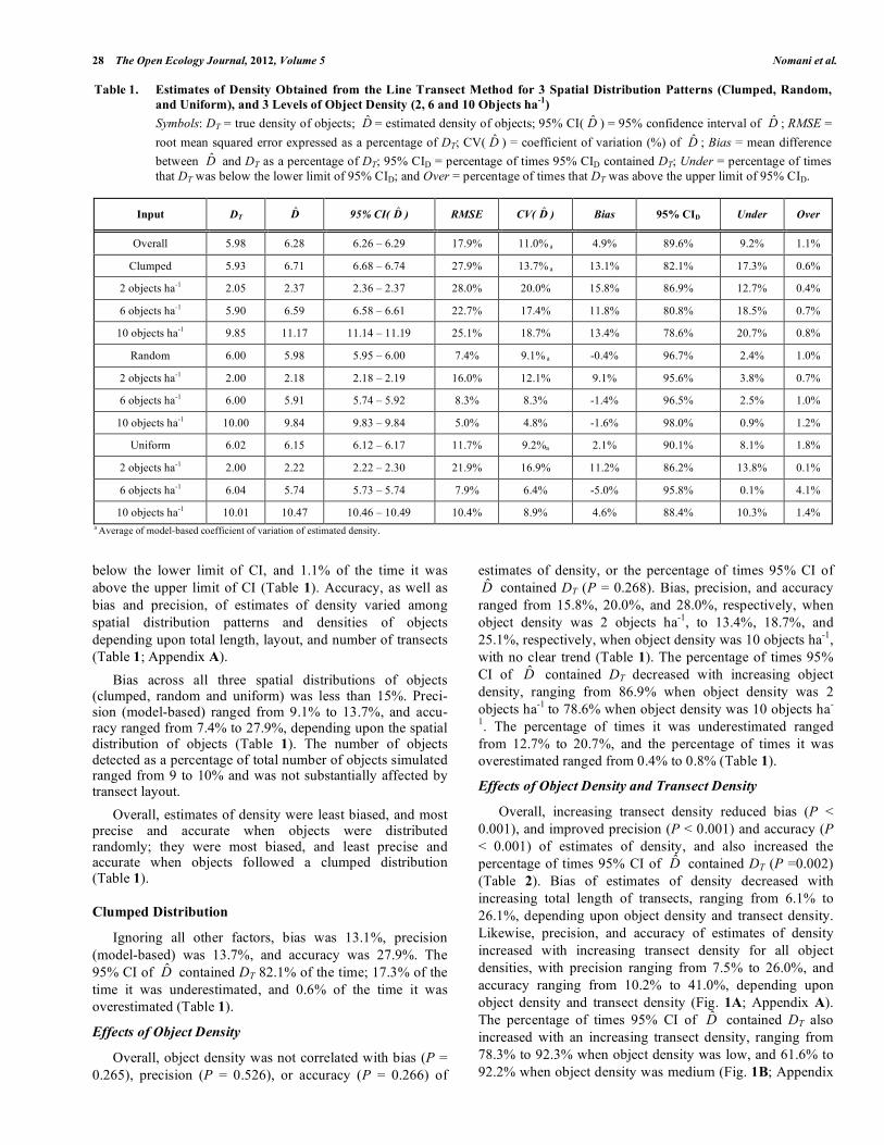
Ignoring all factors (spatial distribution and density of objects, and total length, layout, and number of transects) bias, precision (model-based), and accuracy was 4.9%, 11.0%, and 17.9%, respectively (Table 1). The 95% CI of D̂ contained DT 89.6% of the time; 9.2% of the time it was
28 The Open Ecology Journal, 2012, Volume 5 Nomani et al.
below the lower limit of CI, and 1.1% of the time it was above the upper limit of CI (Table 1). Accuracy, as well as bias and precision, of estimates of density varied among spatial distribution patterns and densities of objects depending upon total length, layout, and number of transects (Table 1; Appendix A). Bias across all three spatial distributions of objects (clumped, random and uniform) was less than 15%. Preci-sion (model-based) ranged from 9.1% to 13.7%, and accu-racy ranged from 7.4% to 27.9%, depending upon the spatial distribution of objects (Table 1). The number of objects detected as a percentage of total number of objects simulated ranged from 9 to 10% and was not substantially affected by transect layout. Overall, estimates of density were least biased, and most precise and accurate when objects were distributed randomly; they were most biased, and least precise and accurate when objects followed a clumped distribution (Table 1).
Clumped Distribution
Ignoring all other factors, bias was 13.1%, precision (model-based) was 13.7%, and accuracy was 27.9%. The 95% CI of D̂ contained DT 82.1% of the time; 17.3% of the time it was underestimated, and 0.6% of the time it was overestimated (Table 1).
Effects of Object Density
Overall, object density was not correlated with bias (P = 0.265), precision (P = 0.526), or accuracy (P = 0.266) of
estimates of density, or the percentage of times 95% CI of D̂ contained DT (P = 0.268). Bias, precision, and accuracy ranged from 15.8%, 20.0%, and 28.0%, respectively, when object density was 2 objects ha-1, to 13.4%, 18.7%, and 25.1%, respectively, when object density was 10 objects ha-1, with no clear trend (Table 1). The percentage of times 95% CI of D̂ contained DT decreased with increasing object density, ranging from 86.9% when object density was 2 objects ha-1 to 78.6% when object density was 10 objects ha-
1. The percentage of times it was underestimated ranged from 12.7% to 20.7%, and the percentage of times it was overestimated ranged from 0.4% to 0.8% (Table 1).
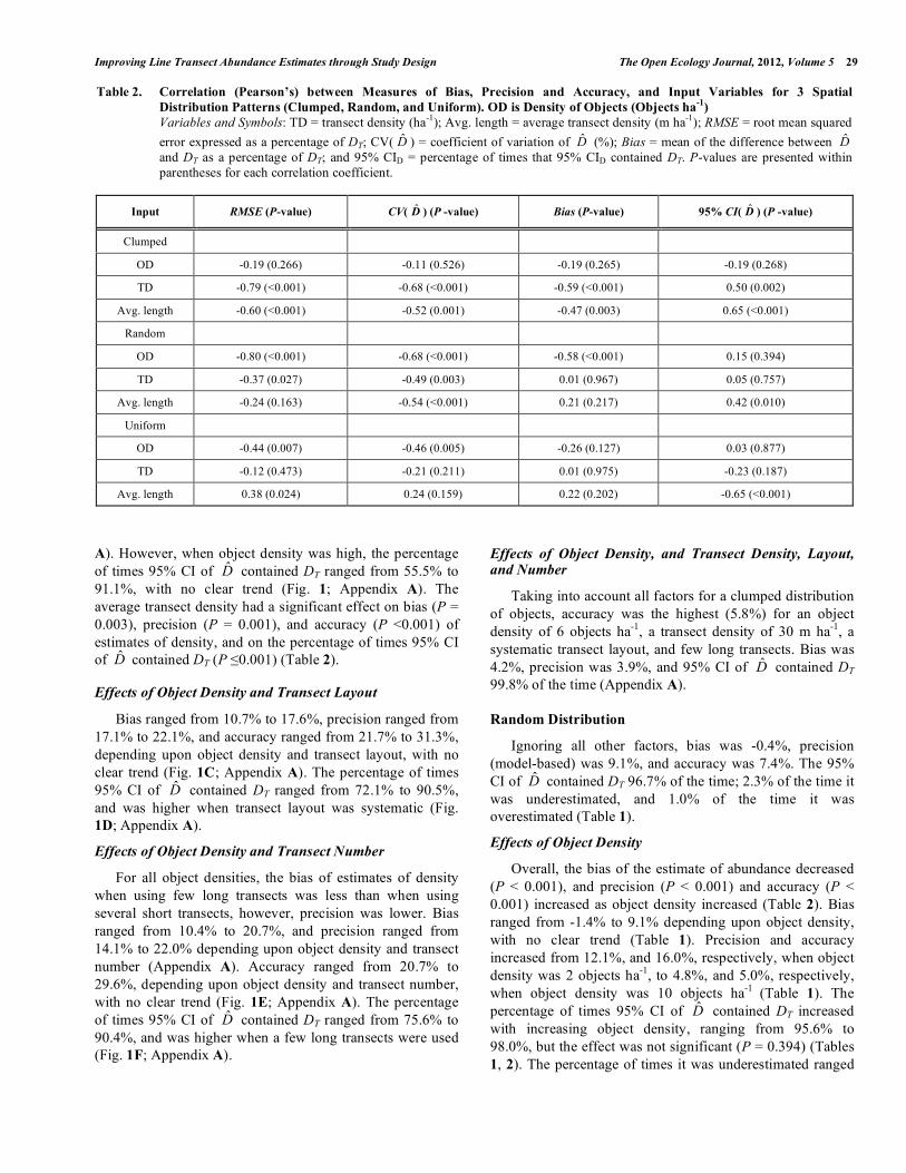
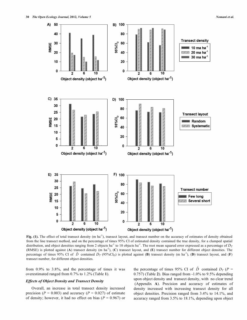
Effects of Object Density and Transect Density
Overall, increasing transect density reduced bias (P < 0.001), and improved precision (P < 0.001) and accuracy (P < 0.001) of estimates of density, and also increased the percentage of times 95% CI of D̂ contained DT (P =0.002) (Table 2). Bias of estimates of density decreased with increasing total length of transects, ranging from 6.1% to 26.1%, depending upon object density and transect density. Likewise, precision, and accuracy of estimates of density increased with increasing transect density for all object densities, with precision ranging from 7.5% to 26.0%, and accuracy ranging from 10.2% to 41.0%, depending upon object density and transect density (Fig. 1A; Appendix A). The percentage of times 95% CI of D̂ contained DT also increased with an increasing transect density, ranging from 78.3% to 92.3% when object density was low, and 61.6% to 92.2% when object density was medium (Fig. 1B; Appendix
Table 1. Estimates of Density Obtained from the Line Transect Method for 3 Spatial Distribution Patterns (Clumped, Random, and Uniform), and 3 Levels of Object Density (2, 6 and 10 Objects ha-1) Symbols: DT = true density of objects; D̂ = estimated density of objects; 95% CI( D̂ ) = 95% confidence interval of D̂ ; RMSE = root mean squared error expressed as a percentage of DT; CV( D̂ ) = coefficient of variation (%) of D̂ ; Bias = mean difference between D̂ and DT as a percentage of DT; 95% CID = percentage of times 95% CID contained DT; Under = percentage of times that DT was below the lower limit of 95% CID; and Over = percentage of times that DT was above the upper limit of 95% CID.
Input DT D̂ 95% CI( D̂ ) RMSE CV( D̂ ) Bias 95% CID Under Over
10 objects ha-1 10.01 10.47 10.46 – 10.49 10.4% 8.9% 4.6% 88.4% 10.3% 1.4% a Average of model-based coefficient of variation of estimated density.
Improving Line Transect Abundance Estimates through Study Design The Open Ecology Journal, 2012, Volume 5 29
A). However, when object density was high, the percentage of times 95% CI of D̂ contained DT ranged from 55.5% to 91.1%, with no clear trend (Fig. 1; Appendix A). The average transect density had a significant effect on bias (P = 0.003), precision (P = 0.001), and accuracy (P <0.001) of estimates of density, and on the percentage of times 95% CI of D̂ contained DT (P ≤0.001) (Table 2).
Effects of Object Density and Transect Layout
Bias ranged from 10.7% to 17.6%, precision ranged from 17.1% to 22.1%, and accuracy ranged from 21.7% to 31.3%, depending upon object density and transect layout, with no clear trend (Fig. 1C; Appendix A). The percentage of times 95% CI of D̂ contained DT ranged from 72.1% to 90.5%, and was higher when transect layout was systematic (Fig. 1D; Appendix A).
Effects of Object Density and Transect Number
For all object densities, the bias of estimates of density when using few long transects was less than when using several short transects, however, precision was lower. Bias ranged from 10.4% to 20.7%, and precision ranged from 14.1% to 22.0% depending upon object density and transect number (Appendix A). Accuracy ranged from 20.7% to 29.6%, depending upon object density and transect number, with no clear trend (Fig. 1E; Appendix A). The percentage of times 95% CI of D̂ contained DT ranged from 75.6% to 90.4%, and was higher when a few long transects were used (Fig. 1F; Appendix A).
Effects of Object Density, and Transect Density, Layout, and Number
Taking into account all factors for a clumped distribution of objects, accuracy was the highest (5.8%) for an object density of 6 objects ha-1, a transect density of 30 m ha-1, a systematic transect layout, and few long transects. Bias was 4.2%, precision was 3.9%, and 95% CI of D̂ contained DT 99.8% of the time (Appendix A).
Random Distribution
Ignoring all other factors, bias was -0.4%, precision (model-based) was 9.1%, and accuracy was 7.4%. The 95% CI of D̂ contained DT 96.7% of the time; 2.3% of the time it was underestimated, and 1.0% of the time it was overestimated (Table 1).
Effects of Object Density
Overall, the bias of the estimate of abundance decreased (P < 0.001), and precision (P < 0.001) and accuracy (P < 0.001) increased as object density increased (Table 2). Bias ranged from -1.4% to 9.1% depending upon object density, with no clear trend (Table 1). Precision and accuracy increased from 12.1%, and 16.0%, respectively, when object density was 2 objects ha-1, to 4.8%, and 5.0%, respectively, when object density was 10 objects ha-1 (Table 1). The percentage of times 95% CI of D̂ contained DT increased with increasing object density, ranging from 95.6% to 98.0%, but the effect was not significant (P = 0.394) (Tables 1, 2). The percentage of times it was underestimated ranged
Table 2. Correlation (Pearson’s) between Measures of Bias, Precision and Accuracy, and Input Variables for 3 Spatial Distribution Patterns (Clumped, Random, and Uniform). OD is Density of Objects (Objects ha-1)
Variables and Symbols: TD = transect density (ha-1); Avg. length = average transect density (m ha-1); RMSE = root mean squared error expressed as a percentage of DT; CV( D̂ ) = coefficient of variation of D̂ (%); Bias = mean of the difference between D̂ and DT as a percentage of DT; and 95% CID = percentage of times that 95% CID contained DT. P-values are presented within parentheses for each correlation coefficient.
30 The Open Ecology Journal, 2012, Volume 5 Nomani et al.
from 0.9% to 3.8%, and the percentage of times it was overestimated ranged from 0.7% to 1.2% (Table 1).
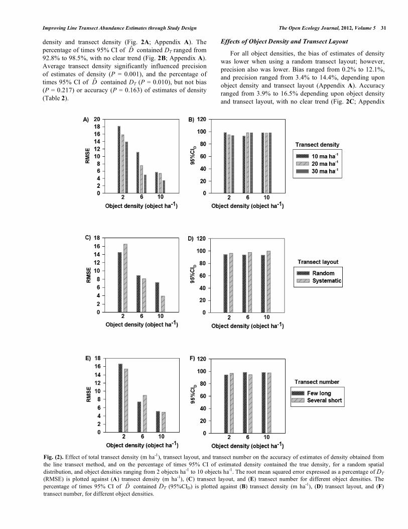
Effects of Object Density and Transect Density
Overall, an increase in total transect density increased precision (P = 0.003) and accuracy (P = 0.027) of estimate of density; however, it had no effect on bias (P = 0.967) or
the percentage of times 95% CI of D̂ contained DT (P = 0.757) (Table 2). Bias ranged from -1.0% to 9.5% depending upon object density and transect density, with no clear trend (Appendix A). Precision and accuracy of estimates of density increased with increasing transect density for all object densities. Precision ranged from 3.4% to 14.1%, and accuracy ranged from 3.5% to 18.1%, depending upon object
Fig. (1). The effect of total transect density (m ha-1), transect layout, and transect number on the accuracy of estimates of density obtained from the line transect method, and on the percentage of times 95% CI of estimated density contained the true density, for a clumped spatial distribution, and object densities ranging from 2 objects ha-1 to 10 objects ha-1. The root mean squared error expressed as a percentage of DT (RMSE) is plotted against (A) transect density (m ha-1), (C) transect layout, and (E) transect number for different object densities. The percentage of times 95% CI of D̂ contained DT (95%CID) is plotted against (B) transect density (m ha-1), (D) transect layout, and (F) transect number, for different object densities.
Improving Line Transect Abundance Estimates through Study Design The Open Ecology Journal, 2012, Volume 5 31
density and transect density (Fig. 2A; Appendix A). The percentage of times 95% CI of D̂ contained DT ranged from 92.8% to 98.5%, with no clear trend (Fig. 2B; Appendix A). Average transect density significantly influenced precision of estimates of density (P = 0.001), and the percentage of times 95% CI of D̂ contained DT (P = 0.010), but not bias (P = 0.217) or accuracy (P = 0.163) of estimates of density (Table 2).
Effects of Object Density and Transect Layout
For all object densities, the bias of estimates of density was lower when using a random transect layout; however, precision also was lower. Bias ranged from 0.2% to 12.1%, and precision ranged from 3.4% to 14.4%, depending upon object density and transect layout (Appendix A). Accuracy ranged from 3.9% to 16.5% depending upon object density and transect layout, with no clear trend (Fig. 2C; Appendix
Fig. (2). Effect of total transect density (m ha-1), transect layout, and transect number on the accuracy of estimates of density obtained from the line transect method, and on the percentage of times 95% CI of estimated density contained the true density, for a random spatial distribution, and object densities ranging from 2 objects ha-1 to 10 objects ha-1. The root mean squared error expressed as a percentage of DT (RMSE) is plotted against (A) transect density (m ha-1), (C) transect layout, and (E) transect number for different object densities. The percentage of times 95% CI of D̂ contained DT (95%CID) is plotted against (B) transect density (m ha-1), (D) transect layout, and (F) transect number, for different object densities.
32 The Open Ecology Journal, 2012, Volume 5 Nomani et al.
A). The percentage of times 95% CI of D̂ contained DT ranged from 93.1% to 99.6%, and was higher when using a systematic transect layout (Fig. 2D; Appendix A).
Effects of Object Density and Transect Number
For all levels of object densities, there was no clear trend in the effect of transect number on bias, precision, or accuracy of estimates of density. Bias ranged from -0.9% to 9.9%, precision ranged from 4.6% to 12.2%, and accuracy ranged from 4.9% to 16.6%, depending upon object density and transect number, with no clear trend (Fig. 2E; Appendix A). The percentage of times 95% CI of D̂ contained DT ranged from 94.3% to 98.4%, with no clear trend (Fig. 2F; Appendix A).
Effects of Object Density, and Transect Density, Layout, and Number
Taking into account all factors for a random distribution of objects, accuracy was highest (2.4%) for an object density of 10 objects ha-1, a transect density of 30 m ha-1, a syste-matic transect layout, and few long transects. Bias was -0.8%, precision was 2.3%, and 95% CI of D̂ contained DT 100% of the time (Appendix A).
Uniform Distribution
Ignoring all other factors, bias was 2.1%, precision (model-based) was 9.2%, and accuracy was 11.7%. The 95% CI of D̂ contained DT 90.1% of the time; 8.1% of the time it was underestimated, and 1.8% of the time it was overestimated (Table 1).
Effects of Object Density
Overall, an increase in object density improved precision (P = 0.005) and accuracy (P = 0.007), but it did not have a significant effect on bias (P = 0.127) and on the percentage of times 95% CI of D̂ contained DT (P = 0.877) (Table 2). Bias ranged from 4.6% to 11.2%, depending upon object density, and decreased with increasing object density (Table 1). Precision ranged from 6.4% to 16.9%, and accuracy ranged from 7.9% to 21.9%, depending upon object density, with no clear trend (Table 1). The percentage of times 95% CI of D̂ contained DT ranged from 86.2% to 95.8%, with no clear trend. The percentage of times it was underestimated ranged from 0.1% to 13.8%, and the percentage of times if was overestimated ranged from 0.1% to 4.1% (Table 1).
Effects of Object Density and Transect Density
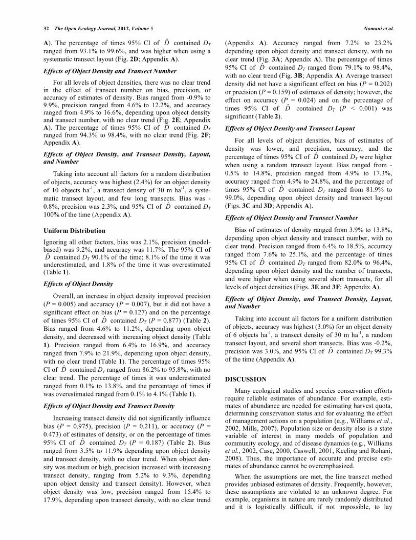
Increasing transect density did not significantly influence bias (P = 0.975), precision (P = 0.211), or accuracy (P = 0.473) of estimates of density, or on the percentage of times 95% CI of D̂ contained DT (P = 0.187) (Table 2). Bias ranged from 3.5% to 11.9% depending upon object density and transect density, with no clear trend. When object den-sity was medium or high, precision increased with increasing transect density, ranging from 5.2% to 9.3%, depending upon object density and transect density). However, when object density was low, precision ranged from 15.4% to 17.9%, depending upon transect density, with no clear trend
(Appendix A). Accuracy ranged from 7.2% to 23.2% depending upon object density and transect density, with no clear trend (Fig. 3A; Appendix A). The percentage of times 95% CI of D̂ contained DT ranged from 79.1% to 98.4%, with no clear trend (Fig. 3B; Appendix A). Average transect density did not have a significant effect on bias (P = 0.202) or precision (P = 0.159) of estimates of density; however, the effect on accuracy (P = 0.024) and on the percentage of times 95% CI of D̂ contained DT (P < 0.001) was significant (Table 2).
Effects of Object Density and Transect Layout
For all levels of object densities, bias of estimates of density was lower, and precision, accuracy, and the percentage of times 95% CI of D̂ contained DT were higher when using a random transect layout. Bias ranged from -0.5% to 14.8%, precision ranged from 4.9% to 17.3%, accuracy ranged from 4.9% to 24.8%, and the percentage of times 95% CI of D̂ contained DT ranged from 81.9% to 99.0%, depending upon object density and transect layout (Figs. 3C and 3D; Appendix A).
Effects of Object Density and Transect Number
Bias of estimates of density ranged from 3.9% to 13.8%, depending upon object density and transect number, with no clear trend. Precision ranged from 6.4% to 18.5%, accuracy ranged from 7.6% to 25.1%, and the percentage of times 95% CI of D̂ contained DT ranged from 82.0% to 96.4%, depending upon object density and the number of transects, and were higher when using several short transects, for all levels of object densities (Figs. 3E and 3F; Appendix A).
Effects of Object Density, and Transect Density, Layout, and Number
Taking into account all factors for a uniform distribution of objects, accuracy was highest (3.0%) for an object density of 6 objects ha-1, a transect density of 30 m ha-1, a random transect layout, and several short transects. Bias was -0.2%, precision was 3.0%, and 95% CI of D̂ contained DT 99.3% of the time (Appendix A).
DISCUSSION
Many ecological studies and species conservation efforts require reliable estimates of abundance. For example, esti-mates of abundance are needed for estimating harvest quota, determining conservation status and for evaluating the effect of management actions on a population (e.g., Williams et al., 2002, Mills, 2007). Population size or density also is a state variable of interest in many models of population and community ecology, and of disease dynamics (e.g., Williams et al., 2002, Case, 2000, Caswell, 2001, Keeling and Rohani, 2008). Thus, the importance of accurate and precise esti-mates of abundance cannot be overemphasized. When the assumptions are met, the line transect method provides unbiased estimates of density. Frequently, however, these assumptions are violated to an unknown degree. For example, organisms in nature are rarely randomly distributed and it is logistically difficult, if not impossible, to lay
Improving Line Transect Abundance Estimates through Study Design The Open Ecology Journal, 2012, Volume 5 33
transect lines randomly. Thus, it is instructive to know whether and to what extent violation of the key assumptions influence accuracy and precision of density estimates, and whether or not it is possible to reduce bias, and improve accuracy and precision of density estimates through study design (e.g., by altering total length, layout, and the number of transects). This, however, requires an understanding of how total length, layout, and the number of transects inf-
luence accuracy and precision of estimates of densities, and of how these influences might vary depending upon the spatial distribution pattern and density of study objects. In this study, we investigated the influence of total length, lay-out, and number of transects on bias, precision, and accuracy of estimates of density for different spatial distribution pat-terns and densities of objects. Specifically, we asked the following questions: (1) How does accuracy and precision of
Fig. (3). Effect of total transect density (m ha-1), transect layout, and transect number on accuracy of estimates of density obtained from the line transect method, and on the percentage of times 95% CI of estimated density contained the true density, for a uniform spatial distribution, and object densities ranging from 2 objects ha-1 to 10 objects ha-1. The root mean squared error expressed as a percentage of DT (RMSE) is plotted against (A) transect density (m ha-1), (C) transect layout, and (E) transect number for different object densities. The percentage of times 95% CI of D̂ contained DT (95%CID) is plotted against (B) transect density (m ha-1), (D) transect layout, and (F) transect number, for different object densities.
34 The Open Ecology Journal, 2012, Volume 5 Nomani et al.
estimates of abundance obtained from the line transect method vary across spatial distribution patterns? (2) How might these patterns be influenced by density of objects? (3) For a given spatial distribution and density level, how do layout, total length, and the number of transects influence accuracy and precision of density estimates? Estimates of density obtained from the line transect method were within 4.9% of the true density, but varied substantially depending upon spatial distribution pattern of objects (Table 1). Overall, the line transect method worked best when objects were distributed randomly. All else being equal, bias was lowest, and precision and accuracy were highest when objects followed a random distribution. Addi-tionally, 95% CI contained true density over 95% of the time (and in cases, as frequently as 98%) of the time (Table 1; Fig. 2). Consequently, it is reasonable to conclude that the line transect method may be most appropriate for estimating abundance when objects or organisms approximate a random distribution pattern. In contrast, the line transect method was most biased, and least accurate and precise when objects followed a clumped spatial distribution pattern (Table 1; Fig. 1). Additionally, the percentage of times 95% CI of estima-ted density contained true density was smaller than expected, sometimes ≤80% of the time. These findings suggest that caution must be exercised when interpreting point estimates as well as confidence intervals of these estimates, particu-larly when objects follow a clumped distribution pattern. When the distribution pattern of objects was clumped, there was no clear trend for the effect of object density on bias, precision, or accuracy of estimates of density. The percentage of times 95% CI of estimated density contained true density decreased with increasing object density (Table 1), but object density did not have a significant effect on bias, precision, or accuracy of estimates of density, or on the percentage of times 95% CI of estimated density contained true density (Table 2). When objects were distributed ran-domly, accuracy of estimates of density increased with increasing object density. Precision of estimates of density increased with increasing object density; however, there was no clear trend in bias of estimates of density. The percentage of times 95% CI of estimated density contained true density increased with increasing object density (Table 1). Object density had a significant effect on bias, precision, and accuracy of estimates of density, however, the effect on the percentage of times 95% CI of estimated density contained true density was not significant (Table 2). When objects were distributed uniformly, bias of estimates of density increased with increasing object density, but there was no clear trend for the effect of object density on precision, or accuracy of estimates of density, or on the percentage of times 95% CI of estimates density contained true density (Table 1). Object density had a significant effect on precision and accuracy of estimates of density, and the effect on bias and on the percentage of times 95% CI contained true density, was not significant (Table 2). The results of our study were consistent with most of our hypotheses. The line transect method worked best when objects followed a random spatial distribution. However, accuracy of estimates of density was less than desired for a clumped distribution of objects (RMSE = 27.9%; Table 1).
For a random distribution of objects, precision of estimates of density increased with increasing object density; however, when object distribution was clumped or uniform, there was no clear trend in the effect of object density on precision of estimates of density. Consistent with our hypothesis, accu-racy of estimates of density increased with an increasing total length of transects for random and clumped distri-butions (Figs. 1A and 2A). Specifically, for a clumped distri-bution, there was a significant increase in accuracy, and a significant decrease in bias of estimates of density for all levels of object density when transect density increased from 10 to 20 m ha-1 (Fig. 1A; Appendix A). However, for a uniform distribution of objects, there was no clear trend in the effect of transect density on accuracy of estimates of density (Fig. 3A). For a clumped distribution, transect layout did not seem to have a substantial effect on bias, precision, or accuracy of estimates of density for all values of object densities (Fig. 1C; Appendix A). For a given total transect density, using several short (as opposed to few long) transects provided greater precision when objects approximated a clumped spatial distribution pattern. Additionally, using several short transects provided slightly greater accuracy when object density was medium, or high. However, bias of estimates was lower when using few long transects for all object densities (Appendix A). Consistent with our hypothesis, a random transect layout worked very well when objects were distributed randomly or uniformly (Figs. 2C, 2D, 3D, and 3C; Appendix A). Buckland et al. (2001) discuss in detail the importance of replication of transects, and stress that a minimum of 10 to 20 replicate lines should be surveyed to provide a basis for adequate variance estimation. In our study, the average number of transects simulated for each of the three spatial distributions (clumped, random, and uniform) was approxi-mately 11 and 18 when using few long transects and several short transects, respectively. A systematic placement of lines has been suggested to provide a better spatial coverage and precision of estimates of density when objects are randomly and independently distributed (Buckland et al., 2001). In our study, transect layout did not influence the number of objects detected (as a percentage of the total number of objects simulated), but significantly influenced precision of esti-mates of abundance, especially when objects were distri-buted randomly or uniformly (Appendix A). For random and clumped distribution patterns, a systematic transect layout provided a slightly greater precision regardless of density of objects, but there was no clear trend for the effect of transect layout on accuracy, precision, or bias of estimates of abundance when objects were distributed uniformly (Fig. 3; Appendix A). When objects followed a random distribution, results were very similar when using a systematic and a random transect layout for all levels of object density (Fig. 2; Appendix A). For uniformly distributed objects, the line transect method worked better when using a random than a systematic transect layout (Fig. 3; Appendix A). When objects followed a clumped distribution, results did not vary substantially based on the pattern of transect layout (syste-matic or random), although the percentage of times that 95% CI of estimated density contained true density was higher for a systematic transect layout (Fig. 1; Appendix A).
Improving Line Transect Abundance Estimates through Study Design The Open Ecology Journal, 2012, Volume 5 35
Fowler (1986) found that the total length of transects did not significantly influence the accuracy of estimates of density; however, precision was variable with the smallest transect density providing the least precise estimates of den-sity. In our study, average transect density had a significant effect on accuracy of estimates of density when distribution of objects was clumped or uniform, and on precision of estimates of density when distribution of objects was clumped or random (Table 2). For a clumped and random distribution, accuracy and precision of estimates of density and 95% CI coverage of DT generally increased with an increasing transect density for all object densities (Figs. 1-2; Appendix A). However, an increase in transect density did not significantly influence the accuracy, but improved the precision, of estimates of density (Fig. 3; Appendix A). Our study further corroborates the claim that the line transect method provides unbiased and precise estimates of abundance when assumptions of the method are met and sample sizes are adequate (Buckland et al., 2001, Williams et al., 2002). However, it is rarely possible to strictly meet all the assumptions of this method or to obtain large sample sizes while sampling animal populations due to time and resource limitations, inaccessibility of the study site or other logistic difficulties. Under such situations, our study shows that accuracy and precision of estimates of abundance can be improved by considering spatial distribution pattern and by appropriately modifying the study design. Spatial distribu-tion of organisms is influenced by a suite of factors that may include habitat, food availability, and behavioral mecha-nisms. A given species may not always follow a particular distribution pattern, and researchers can usually observe but not manipulate distribution and density of organisms. Nonetheless, a knowledge of the relative performance of the line transect method under the various spatial distribution patterns dictated by ecological constraints can help resear-chers to identify potential limitations of the method, and suggest study designs that could help reduce bias and improve precision and accuracy of the estimates of density. We found that, overall, the line transect method was most effective for random, and least effective for a clumped distribution of objects. These results are of critical import-ance because the spatial distribution patterns of many orga-nisms tend to be non-random. Virtually all social animals follow clumped distribution, as do many other species that seek resources that are patchily distributed (Chapman, 1988, Burgess et al., 1982, Cornelissen and Stiling, 2008). Calambokidis et al. (2004) noted the difficulties in using line transect method for estimating abundance of near-shore, humpback and blue whales that exhibit clumped distribution pattern, and Buckland et al. (2007) suggested new app-roaches for estimating abundance of strongly aggregated plant populations. Our study shows that, when spatial distri-bution of objects is clumped or random, precision and accu-racy of estimates of density obtained from the line transect method can generally be improved by increasing total length of transects, and by laying out the transects systematically. We also recommend using several short, rather than few long, transects, because this approach can help reduce bias
and increase precision. Finally, we note that the line transect method can potentially underestimate abundance if spatial distribution of objects are nonrandom, and especially when distribution is clumped. The line transect method is often the most efficient and cost-effective method of estimating popu-lation sizes (e.g., Nomani et al., 2008), and results presented in this paper will help refine the study design to maximize accuracy and precision of estimates of abundance based on the line transect method under conditions in the field. The line transect method has been the method of choice for estimating abundance for many taxa because it adequa-tely addresses two major challenges in abundance estima-tion: spatial sampling and detectability (Williams et al., 2002). Furthermore, compared to alternative approaches such as capture-recapture or total count, this method is efficient and cost effective (Williams et al., 2002, Buckland et al., 2001, Buckland et al., 2007, Nomani et al., 2008). However, conventional approaches to abundance estimation based on line transect distance sampling do not permit modeling abundance as a function of environmental cova-riates that can affect both spatial distribution pattern and population density. To this end, it is encouraging to note that modeling approaches such as the hierarchical modeling framework of Royle et al. (2004), and its extension to allow temporary emigration (Chandler et al., 2011), will prove useful to improve accuracy and precision of density estimates and statistical inference regarding covariate effects on density. Finally, the availability of software packages such as unmarked (Fiske et al., 2012) will facilitate the implementation of recently developed density estimation and modeling approaches using data collected from distance sampling. Careful study design as per our recommendations, along with the application of recently developed modeling approaches to analyze and model the resulting data (Chandler et al., 2011, Royle et al., 2004) will undoubtedly help improve accuracy and precision of estimates of abundance using distance sampling methods.
CONFLICT OF INTEREST
None declared.
ACKNOWLEDGEMENTS
The Department of Wildlife Ecology and Conservation at the University of Florida provided funding for this project. Institutional IACUC consultation designated the study as primarily observational and no review was required. We thank I. Ismail, A. Jaffery, A. Ozgul, J. Hostetler, K. Aaltonen, A. Singh, and especially J. D. Nichols and G. C. White for insightful comments on the manuscript, and for assistance with statistical analysis. Special thanks go to L. Thomas, S. Buckland, N. Adams, H. Sultan, M. Christman, M. Sitharam, and J. D. Nichols for their help with the design and implementation of the simulation programs. Any use of trade, product or firm names is for descriptive purposes only and does not imply endorsement by the U.S. Government.
36 The Open Ecology Journal, 2012, Volume 5 Nomani et al.
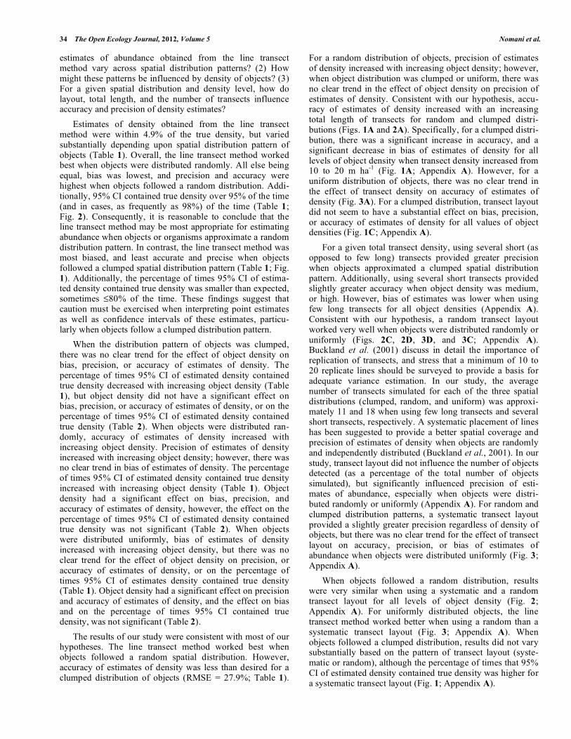
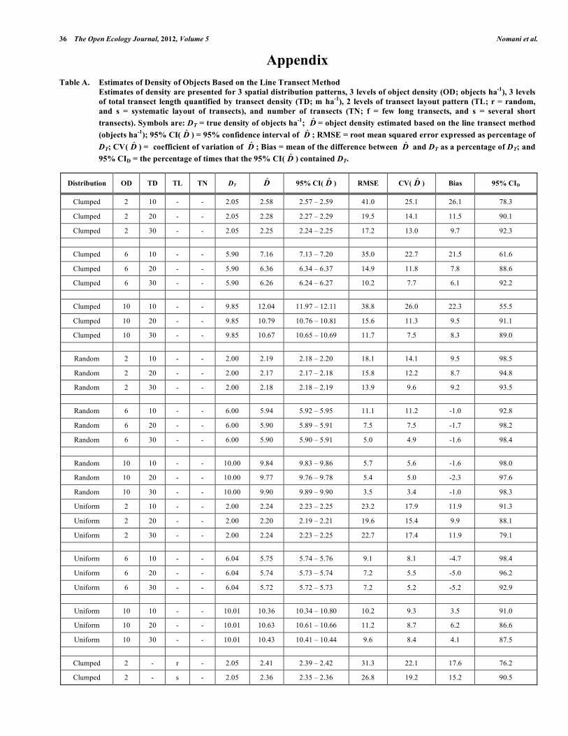
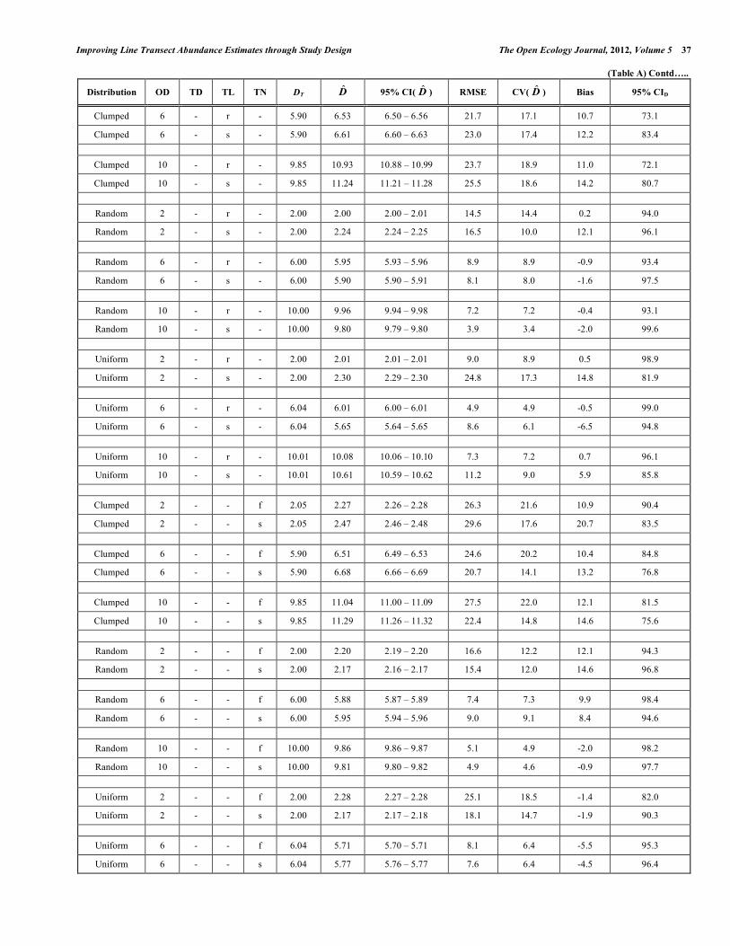
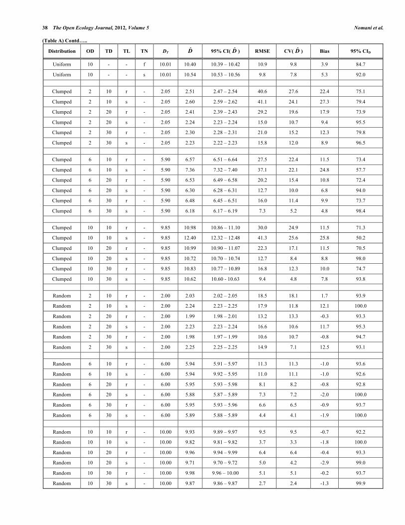
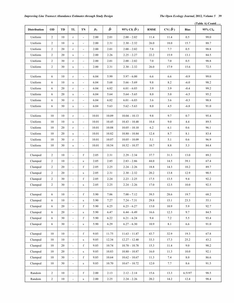
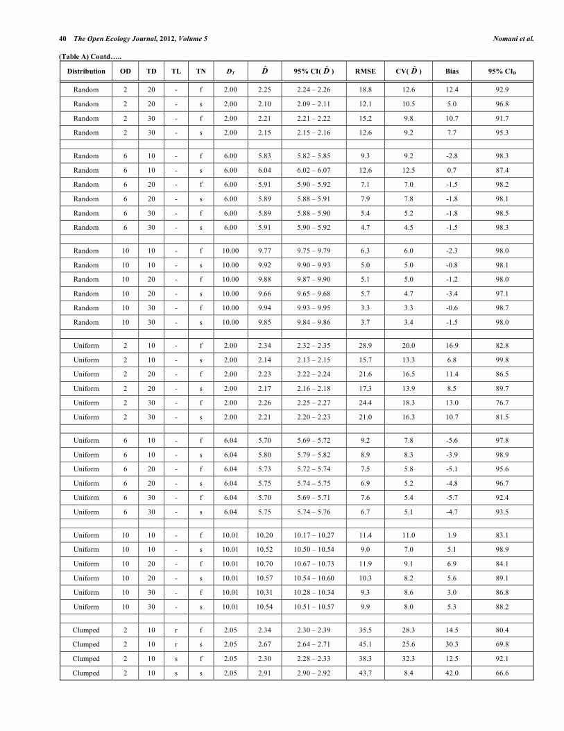
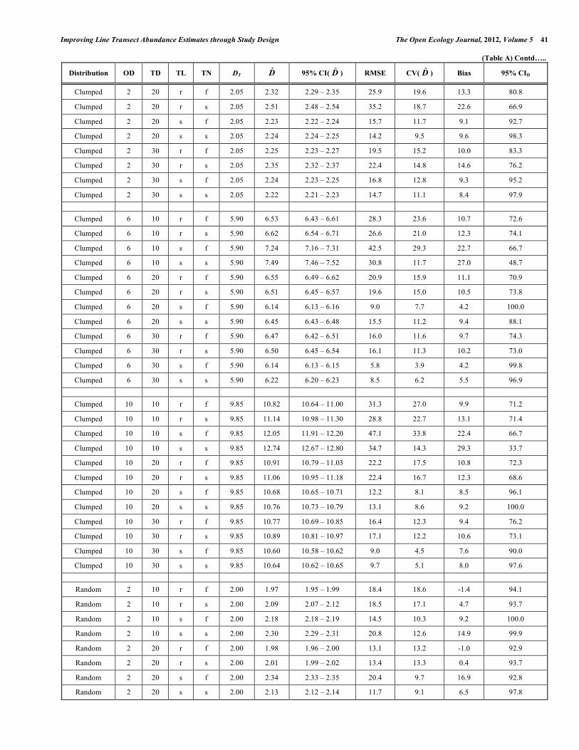
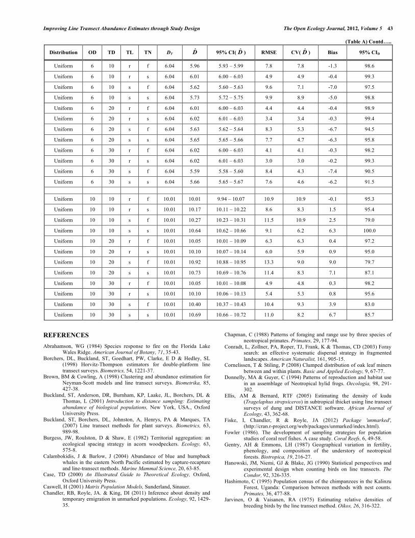
Appendix Table A. Estimates of Density of Objects Based on the Line Transect Method Estimates of density are presented for 3 spatial distribution patterns, 3 levels of object density (OD; objects ha-1), 3 levels
of total transect length quantified by transect density (TD; m ha-1), 2 levels of transect layout pattern (TL; r = random, and s = systematic layout of transects), and number of transects (TN; f = few long transects, and s = several short transects). Symbols are: DT = true density of objects ha-1; D̂ = object density estimated based on the line transect method (objects ha-1); 95% CI( D̂ ) = 95% confidence interval of D̂ ; RMSE = root mean squared error expressed as percentage of DT; CV( D̂ ) = coefficient of variation of D̂ ; Bias = mean of the difference between D̂ and DT as a percentage of DT; and 95% CID = the percentage of times that the 95% CI( D̂ ) contained DT.
Distribution OD TD TL TN DT D̂ 95% CI( D̂ ) RMSE CV( D̂ ) Bias 95% CID
Clumped 2 10 r f 2.05 2.34 2.30 – 2.39 35.5 28.3 14.5 80.4
Clumped 2 10 r s 2.05 2.67 2.64 – 2.71 45.1 25.6 30.3 69.8
Clumped 2 10 s f 2.05 2.30 2.28 – 2.33 38.3 32.3 12.5 92.1
Clumped 2 10 s s 2.05 2.91 2.90 – 2.92 43.7 8.4 42.0 66.6
Improving Line Transect Abundance Estimates through Study Design The Open Ecology Journal, 2012, Volume 5 41 (Table A) Contd…..
Distribution OD TD TL TN DT D̂ 95% CI( D̂ ) RMSE CV( D̂ ) Bias 95% CID
Clumped 2 20 r f 2.05 2.32 2.29 – 2.35 25.9 19.6 13.3 80.8
Clumped 2 20 r s 2.05 2.51 2.48 – 2.54 35.2 18.7 22.6 66.9
Clumped 2 20 s f 2.05 2.23 2.22 – 2.24 15.7 11.7 9.1 92.7
Clumped 2 20 s s 2.05 2.24 2.24 – 2.25 14.2 9.5 9.6 98.3
Clumped 2 30 r f 2.05 2.25 2.23 – 2.27 19.5 15.2 10.0 83.3
Clumped 2 30 r s 2.05 2.35 2.32 – 2.37 22.4 14.8 14.6 76.2
Clumped 2 30 s f 2.05 2.24 2.23 – 2.25 16.8 12.8 9.3 95.2
Clumped 2 30 s s 2.05 2.22 2.21 – 2.23 14.7 11.1 8.4 97.9
Clumped 6 10 r f 5.90 6.53 6.43 – 6.61 28.3 23.6 10.7 72.6
Clumped 6 10 r s 5.90 6.62 6.54 – 6.71 26.6 21.0 12.3 74.1
Clumped 6 10 s f 5.90 7.24 7.16 – 7.31 42.5 29.3 22.7 66.7
Clumped 6 10 s s 5.90 7.49 7.46 – 7.52 30.8 11.7 27.0 48.7
Clumped 6 20 r f 5.90 6.55 6.49 – 6.62 20.9 15.9 11.1 70.9
Clumped 6 20 r s 5.90 6.51 6.45 – 6.57 19.6 15.0 10.5 73.8
Clumped 6 20 s f 5.90 6.14 6.13 – 6.16 9.0 7.7 4.2 100.0
Clumped 6 20 s s 5.90 6.45 6.43 – 6.48 15.5 11.2 9.4 88.1
Clumped 6 30 r f 5.90 6.47 6.42 – 6.51 16.0 11.6 9.7 74.3
Clumped 6 30 r s 5.90 6.50 6.45 – 6.54 16.1 11.3 10.2 73.0
Clumped 6 30 s f 5.90 6.14 6.13 – 6.15 5.8 3.9 4.2 99.8
Clumped 6 30 s s 5.90 6.22 6.20 – 6.23 8.5 6.2 5.5 96.9
Clumped 10 10 r f 9.85 10.82 10.64 – 11.00 31.3 27.0 9.9 71.2
Clumped 10 10 r s 9.85 11.14 10.98 – 11.30 28.8 22.7 13.1 71.4
Clumped 10 10 s f 9.85 12.05 11.91 – 12.20 47.1 33.8 22.4 66.7
Clumped 10 10 s s 9.85 12.74 12.67 – 12.80 34.7 14.3 29.3 33.7
Clumped 10 20 r f 9.85 10.91 10.79 – 11.03 22.2 17.5 10.8 72.3
Clumped 10 20 r s 9.85 11.06 10.95 – 11.18 22.4 16.7 12.3 68.6
Clumped 10 20 s f 9.85 10.68 10.65 – 10.71 12.2 8.1 8.5 96.1
Clumped 10 20 s s 9.85 10.76 10.73 – 10.79 13.1 8.6 9.2 100.0
Clumped 10 30 r f 9.85 10.77 10.69 – 10.85 16.4 12.3 9.4 76.2
Clumped 10 30 r s 9.85 10.89 10.81 – 10.97 17.1 12.2 10.6 73.1
Clumped 10 30 s f 9.85 10.60 10.58 – 10.62 9.0 4.5 7.6 90.0
Clumped 10 30 s s 9.85 10.64 10.62 – 10.65 9.7 5.1 8.0 97.6
Random 2 10 r f 2.00 1.97 1.95 – 1.99 18.4 18.6 -1.4 94.1
Random 2 10 r s 2.00 2.09 2.07 – 2.12 18.5 17.1 4.7 93.7
Random 2 10 s f 2.00 2.18 2.18 – 2.19 14.5 10.3 9.2 100.0
Random 2 10 s s 2.00 2.30 2.29 – 2.31 20.8 12.6 14.9 99.9
Random 2 20 r f 2.00 1.98 1.96 – 2.00 13.1 13.2 -1.0 92.9
Random 2 20 r s 2.00 2.01 1.99 – 2.02 13.4 13.3 0.4 93.7
Random 2 20 s f 2.00 2.34 2.33 – 2.35 20.4 9.7 16.9 92.8
Random 2 20 s s 2.00 2.13 2.12 – 2.14 11.7 9.1 6.5 97.8
42 The Open Ecology Journal, 2012, Volume 5 Nomani et al.
(Table A) Contd…..
Distribution OD TD TL TN DT D̂ 95% CI( D̂ ) RMSE CV( D̂ ) Bias 95% CID
Random 2 30 r f 2.00 1.99 1.98 – 2.00 10.8 10.8 -0.5 94.1
Random 2 30 r s 2.00 1.98 1.96 – 1.99 10.4 10.5 -0.1 95.2
Random 2 30 s f 2.00 2.29 2.28 – 2.29 16.4 6.9 14.4 90.8
Random 2 30 s s 2.00 2.21 2.21 – 2.22 13.2 7.0 10.7 95.4
Random 6 10 r f 6.00 5.90 5.85 – 5.94 11.9 11.9 -1.7 93.3
Random 6 10 r s 6.00 5.98 5.94 – 6.02 10.7 10.7 -0.4 93.8
Random 6 10 s f 6.00 5.81 5.79 – 5.83 8.3 7.9 -3.2 100.0
Random 6 10 s s 6.00 6.06 6.04 – 6.09 13.2 13.1 1.1 85.2
Random 6 20 r f 6.00 5.95 9.92 – 5.98 8.2 8.2 -0.9 93.0
Random 6 20 r s 6.00 5.96 5.93 – 5.99 8.1 8.1 -0.6 92.6
Random 6 20 s f 6.00 5.90 5.88 – 5.91 6.7 6.6 -1.7 100.0
Random 6 20 s s 6.00 5.87 5.85 – 5.89 7.9 7.7 -2.2 100.0
Random 6 30 r f 6.00 5.96 5.94 – 5.99 6.6 6.7 -0.7 94.1
Random 6 30 r s 6.00 5.93 5.91 – 5.95 6.5 6.4 -1.2 93.3
Random 6 30 s f 6.00 5.87 5.86 – 5.88 4.9 4.5 -2.1 100.0
Random 6 30 s s 6.00 5.90 5.90 – 5.91 3.9 3.6 1.6 100.0
Random 10 10 r f 10.00 9.88 9.82 – 9.94 10.0 10.1 -1.2 91.9
Random 10 10 r s 10.00 9.98 9.92 – 10.03 8.9 8.9 -0.2 92.4
Random 10 10 s f 10.00 9.73 9.72 – 9.75 4.5 3.7 -2.7 100.0
Random 10 10 s s 10.00 9.89 9.89 – 9.91 2.7 2.6 -1.0 100.0
Random 10 20 r f 10.00 9.99 9.95 – 10.03 6.5 6.5 -0.1 93.4
Random 10 20 r s 10.00 9.94 9.90 – 9.98 6.2 6.3 -0.6 93.2
Random 10 20 s f 10.00 9.85 9.83 – 9.86 4.5 4.3 -1.5 99.6
Random 10 20 s s 10.00 9.57 9.56 – 9.58 5.5 3.5 -4.3 98.4
Random 10 30 r f 10.00 10.01 9.97 - 10.04 5.1 5.1 0.1 94.8
Random 10 30 r s 10.00 9.96 9.93 – 9.99 5.2 5.2 -0.4 92.6
Random 10 30 s f 10.00 9.92 9.91 – 9.93 2.4 2.3 -0.8 100.0
Random 10 30 s s 10.00 9.82 9.81 – 9.82 3.0 2.4 -1.8 99.7
Uniform 2 10 r f 2.00 1.99 1.97 – 2.00 11.4 11.4 -0.6 98.9
Uniform 2 10 r s 2.00 2.03 2.02 – 2.05 11.5 11.2 1.6 99.1
Uniform 2 10 s f 2.00 2.46 2.44 – 2.47 32.7 19.1 22.8 77.5
Uniform 2 10 s s 2.00 2.17 2.16 – 2.18 16.9 13.4 8.5 100.0
Uniform 2 20 r f 2.00 2.01 2.00 – 2.02 8.0 8.0 0.3 98.6
Uniform 2 20 r s 2.00 2.01 2.01 – 2.02 7.6 7.5 0.7 99.0
Uniform 2 20 s f 2.00 2.30 2.29 – 2.31 24.6 16.9 15.1 82.4
Uniform 2 20 s s 2.00 2.22 2.21 – 2.23 19.5 14.5 11.1 86.6
Uniform 2 30 r f 2.00 2.00 1.99 – 2.01 7.1 7.1 0.2 98.7
Uniform 2 30 r s 2.00 2.02 2.01 – 2.03 6.9 6.8 0.9 98.9
Uniform 2 30 s f 2.00 2.34 2.33 – 2.36 27.9 18.7 17.2 69.4
Uniform 2 30 s s 2.00 2.28 2.27 – 2.29 23.3 17.0 14.0 75.6
Improving Line Transect Abundance Estimates through Study Design The Open Ecology Journal, 2012, Volume 5 43 (Table A) Contd…..
Distribution OD TD TL TN DT D̂ 95% CI( D̂ ) RMSE CV( D̂ ) Bias 95% CID
Uniform 6 10 r f 6.04 5.96 5.93 – 5.99 7.8 7.8 -1.3 98.6
Uniform 6 10 r s 6.04 6.01 6.00 – 6.03 4.9 4.9 -0.4 99.3
Uniform 6 10 s f 6.04 5.62 5.60 – 5.63 9.6 7.1 -7.0 97.5
Uniform 6 10 s s 6.04 5.73 5.72 – 5.75 9.9 8.9 -5.0 98.8
Uniform 6 20 r f 6.04 6.01 6.00 – 6.03 4.4 4.4 -0.4 98.9
Uniform 6 20 r s 6.04 6.02 6.01 – 6.03 3.4 3.4 -0.3 99.4
Uniform 6 20 s f 6.04 5.63 5.62 – 5.64 8.3 5.3 -6.7 94.5
Uniform 6 20 s s 6.04 5.65 5.65 – 5.66 7.7 4.7 -6.3 95.8
Uniform 6 30 r f 6.04 6.02 6.00 – 6.03 4.1 4.1 -0.3 98.2
Uniform 6 30 r s 6.04 6.02 6.01 – 6.03 3.0 3.0 -0.2 99.3
Uniform 6 30 s f 6.04 5.59 5.58 – 5.60 8.4 4.3 -7.4 90.5
Uniform 6 30 s s 6.04 5.66 5.65 – 5.67 7.6 4.6 -6.2 91.5
Uniform 10 10 r f 10.01 10.01 9.94 – 10.07 10.9 10.9 -0.1 95.3
Uniform 10 10 r s 10.01 10.17 10.11 – 10.22 8.6 8.3 1.5 95.4
Uniform 10 10 s f 10.01 10.27 10.23 – 10.31 11.5 10.9 2.5 79.0
Uniform 10 10 s s 10.01 10.64 10.62 – 10.66 9.1 6.2 6.3 100.0
Uniform 10 20 r f 10.01 10.05 10.01 – 10.09 6.3 6.3 0.4 97.2
Uniform 10 20 r s 10.01 10.10 10.07 – 10.14 6.0 5.9 0.9 95.0
Uniform 10 20 s f 10.01 10.92 10.88 – 10.95 13.3 9.0 9.0 79.7
Uniform 10 20 s s 10.01 10.73 10.69 – 10.76 11.4 8.3 7.1 87.1
Uniform 10 30 r f 10.01 10.05 10.01 – 10.08 4.9 4.8 0.3 98.2
Uniform 10 30 r s 10.01 10.10 10.06 – 10.13 5.4 5.3 0.8 95.6
Uniform 10 30 s f 10.01 10.40 10.37 – 10.43 10.4 9.3 3.9 83.0
Uniform 10 30 s s 10.01 10.69 10.66 – 10.72 11.0 8.2 6.7 85.7
REFERENCES Abrahamson, WG (1984) Species response to fire on the Florida Lake
Wales Ridge. American Journal of Botany, 71, 35-43. Borchers, DL, Buckland, ST, Goedhart, PW, Clarke, E D & Hedley, SL
(1998) Horvitz-Thompson estimators for double-platform line transect surveys. Biometrics, 54, 1221-37.
Brown, BM & Cowling, A (1998) Clustering and abundance estimation for Neyman-Scott models and line transect surveys. Biometrika, 85, 427-38.
Buckland, ST, Anderson, DR, Burnham, KP, Laake, JL, Borchers, DL & Thomas, L (2001) Introduction to distance sampling: Estimating abundance of biological populations, New York, USA., Oxford University Press.
Buckland, ST, Borchers, DL, Johnston, A, Henrys, PA & Marques, TA (2007) Line transect methods for plant surveys. Biometrics, 63, 989-98.
Burgess, JW, Roulston, D & Shaw, E (1982) Territorial aggregation: an ecological spacing strategy in acorn woodpeckers. Ecology, 63, 575-8.
Calambokidis, J & Barlow, J (2004) Abundance of blue and humpback whales in the eastern North Pacific estimated by capture-recapture and line-transect methods. Marine Mammal Science, 20, 63-85.
Case, TD (2000) An Illustrated Guide to Theoretical Ecology, Oxford, Oxford University Press.
Caswell, H (2001) Matrix Population Models, Sunderland, Sinauer. Chandler, RB, Royle, JA. & King, DI (2011) Inference about density and
temporary emigration in unmarked populations. Ecology, 92, 1429-35.
Chapman, C (1988) Patterns of foraging and range use by three species of neotropical primates. Primates, 29, 177-94.
Conradt, L, Zollner, PA, Roper, TJ, Frank, K & Thomas, CD (2003) Foray search: an effective systematic dispersal strategy in fragmented landscapes. American Naturalist, 161, 905-15.
Cornelissen, T & Stiling, P (2008) Clumped distribution of oak leaf miners between and within plants. Basic and Applied Ecology, 9, 67-77.
Donnelly, MA & Guyer, C (1994) Patterns of reproduction and habitat use in an assemblage of Neotropical hylid frogs. Oecologia, 98, 291-302.
Ellis, AM & Bernard, RTF (2005) Estimating the density of kudu (Tragelaphus strepsiceros) in subtropical thicket using line transect surveys of dung and DISTANCE software. African Journal of Ecology, 43, 362-68.
Fiske, I, Chandler, R & Royle, JA (2012) Package 'unmarked', (http://cran.r-project.org/web/packages/unmarked/index.html).
Fowler (1986). The development of sampling strategies for population studies of coral reef fishes. A case study. Coral Reefs, 6, 49-58.
Gentry, AH & Emmons, LH (1987) Geographical variation in fertility, phenology, and composition of the understory of neotropical forests. Biotropica, 19, 216-27.
Hanowski, JM, Niemi, GJ & Blake, JG (1990) Statistical perspectives and experimental design when counting birds on line transects. The Condor, 92, 326-335.
Hashimoto, C (1995) Population census of the chimpanzees in the Kalinzu Forest, Uganda: Comparison between methods with nest counts. Primates, 36, 477-88.
Jarvinen, O & Vaisanen, RA (1975) Estimating relative densities of breeding birds by the line transect method. Oikos, 26, 316-322.
44 The Open Ecology Journal, 2012, Volume 5 Nomani et al.
Jefferson, TA (1996) Estimates of abundance of cetaceans in offshore waters by the northwestern Gulf of Mexico, 1992-1993. Southwestern Naturalist, 41, 279-87.
Keeling, MJ & Rohani, P (2008) Modeling infectious diseases in humans and animals., Princeton, Princeton University Press.
Krebs, CJ (1999) Ecological Methodology, Menlo Park, California, USA, Addison-Wesley Educational Publishers.
Krzysik, AJ (2002) A landscape sampling protocol for estimating distribution and density patterns of desert tortoise at multiple spatial scales. Chelonian Conservation and Biology, 4, 366-379.
Lewis, DL, Baxter, GT, Johnson, KM & Stone, MD (1985) Possible extinction of the Wyoming toad, Bufo hemiophrys baxteri. Journal of Herpetology, 19, 166-168.
Lohoefener, R. Line transect estimation of gopher tortoise burrow density using a fourier series. In: Wester, E., Dodd Jr, C. K. & Franz, R., eds. Eighth annual meeting gopher tortoise council, (1990) Florida Museum of Natural History, Gainesville, Florida, USA, pp. 44-69.
Marques, FFC, Buckland, ST, Goffin, D, Dixon, CE, Borchers, DL, Mayle, BA & Peace, AJ (2001) Estimating deer abundance from line transect surveys of dung: sika deer in southern Scotland. Journal of Applied Ecology, 38, 349-63.
This is an open access article licensed under the terms of the Creative Commons Attribution Non-Commercial License (http://creativecommons.org/ licenses/by-nc/3.0/), which permits unrestricted, non-commercial use, distribution and reproduction in any medium, provided the work is properly cited.