Clemson University TigerPrints All eses eses 5-2007 Linear and Non-Linear Control of a Quadrotor UAV Andrew Neff Clemson University, aneff@ieee.org Follow this and additional works at: hps://tigerprints.clemson.edu/all_theses Part of the Electrical and Computer Engineering Commons is esis is brought to you for free and open access by the eses at TigerPrints. It has been accepted for inclusion in All eses by an authorized administrator of TigerPrints. For more information, please contact [email protected]. Recommended Citation Neff, Andrew, "Linear and Non-Linear Control of a Quadrotor UAV" (2007). All eses. 88. hps://tigerprints.clemson.edu/all_theses/88
Transcript
Clemson UniversityTigerPrints
All Theses Theses
5-2007
Linear and Non-Linear Control of a QuadrotorUAVAndrew NeffClemson University, [email protected]
Follow this and additional works at: https://tigerprints.clemson.edu/all_theses
Part of the Electrical and Computer Engineering Commons
This Thesis is brought to you for free and open access by the Theses at TigerPrints. It has been accepted for inclusion in All Theses by an authorizedadministrator of TigerPrints. For more information, please contact [email protected].
Recommended CitationNeff, Andrew, "Linear and Non-Linear Control of a Quadrotor UAV" (2007). All Theses. 88.https://tigerprints.clemson.edu/all_theses/88
An unmanned aerial vehicle (UAV) refers to any flying vehicle that does
not require a live pilot on the aircraft, typically an airplane or helicopter.
UAV research is a growing field because of the emerging affordable technology,
allowing for UAVs to be deployed in numerous new applications. Sending
UAVs into dangerous situations prevents the endangering of human lives while
accomplishing tasks such as visual inspections, following a target [4], scouting,
and many more applications.
This thesis will focus on the control design for a particular UAV, the
quadrotor helicopter, because of its simple design and its ability to control its
torques. This particular type of UAV is an underactuated helicopter that is,
there are only four inputs to control the six degrees-of-freedom. The quadrotor
design is covered in [6] and the analysis for controlling a quadrotor is described
in [11]. Since the quadrotor has only four control inputs, two degrees-of-
freedom are coupled in the sense that the translational position depends on
the orientation of the aircraft.
Another key aspect to developing these control systems is the sensors that
measure position and orientation of an aerial vehicle. One of the most prevalent
sensor systems in use is the global positioning system (GPS) based on satellite
signals. GPS supplies measurements of the three translational positions and
velocities with respect to the earth. However, to measure the three orienta-
tions another technology is required. Using a combination of microelectro-
mechanical systems (MEMS) gyroscopes, accelerometers, and magnetometers,
the orientation of a UAV can be determined. Thus, by combining GPS sensor
with an array of attitude sensors, the six DOF position and orientation of an
aircraft can be determined.
Previous Work
There is a lot of work being done on UAVs with the availability of affordable
UAVs and UAV sensors such as MEMS Gyros and GPS sensors. The Jang
and Tomlin paper [8] discusses the use of a single GPS sensor for use on
UAV tracking. It is important to have a method for a UAV to know where
it is and how it is oriented so that a controller can have a feedback signal.
The Hamel and Mohony paper [3] defines a dynamic model for an X-4 Flyer.
The X-4 Flyer is another quadrotor similar to the DraganFlyer X-Pro used at
Clemson University. The dynamic model proposed in [3] treated the quadrotor
helicopter as a rigid body that has the ability to thrust and torque itself in
midair.
The Chitrakaran and Dawson paper [5] designs an autonomous landing
system using a vision based controller. The controller used includes a method
for handling the underactuated quadrotor and the coupling between the trans-
lational and rotational forces. Procerus Technologies has a Vision-Centric [15]
approach to many targeting systems. They have developed an OnPoint Target-
ing system that include 5 different tracking methods. Among these difference
methods, include a Fly by Camera Control approach where the UAV can be
controlled from the frame of reference of the camera instead of the UAV frame.
Thesis Outline
A MEMS and GPS sensor are used on a quadrotor helicopter in the de-
velopment of two completely different control systems. The first is a PID
controller that will utilize the angular sensors for controlling the orientation of
a quadrotor in flight, according to a set of desired orientations. Hovering a he-
licopter is a very demanding task that requires many small adjustments when
flying by hand and can only be effectively accomplished by an experienced
pilot. Using the proposed orientation controller, the user simply specifies an
orientation, and the control works to achieve it. The desired orientations used
2
can be generated by numerous means, but they will be generated by a joystick
for these experiments.
The second control system will focus on the visual inspection application
of UAVs. When a helicopter is flown, an operator will typically: watch the
helicopter as it moves and actuate the motors for local uses or watch video
taken from a pilot perspective with an on-board video camera. In either case,
it is difficult to manually keep the UAV stable. A new approach to this control
problem was presented in [5] where the UAV and the camera positioning unit
are considered to be a single robotic unit. From this perspective, a controller
can be developed which will simultaneously control both the UAV and the cam-
era positioning unit in a complementary fashion. Here, this control approach
is exploited to provide a new perspective for piloting the UAV. This perspec-
tive, which shall be referred to as the fly-the-camera perspective, presents a
new interface to the pilot. In this proposed approach, the pilot commands
motion from the perspective of the on-board camera - it is as though the pilot
is riding on the tip of the camera and commanding movement of the camera
ala a six-DOF flying camera. This is subtly different from the traditional re-
mote control approach wherein the pilot processes the camera view and then
commands an aircraft motion to create a desired motion of the camera view.
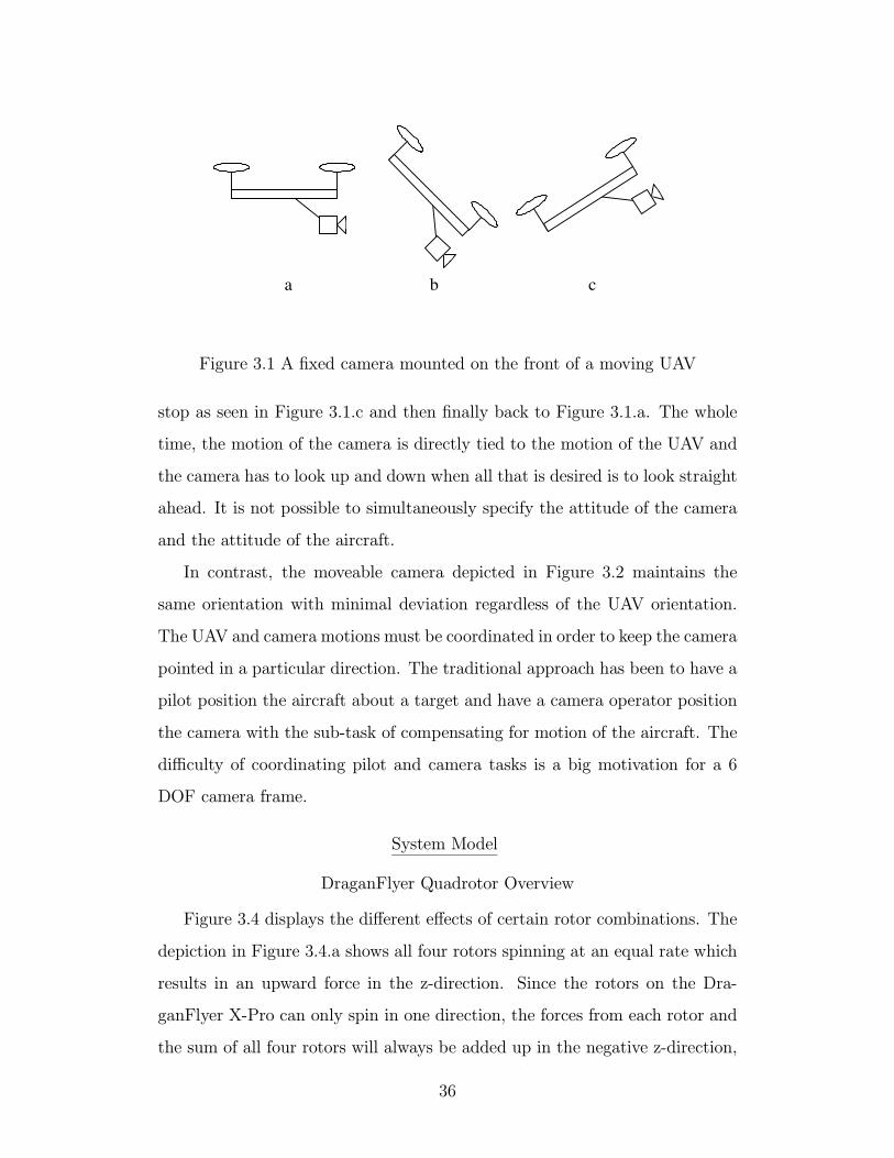
If there is a camera mounted on the UAV, then the orientation and the
position of the UAV affect the orientation and position of the camera. Since
the camera is very important during visual inspections, it was decided that
instead of making the control inputs control the UAV, a non-linear controller
will be used to control the movements of the camera, actuating the UAV in
the process. The control inputs will not be controlling a particular torque to
either keep the UAV still, to rotate it, or to move the UAV, but the input will
simple tell the camera to move in a particular direction, handling the current
orientation of the UAV in the background. In addition, using an actuated
camera and the UAV will create a fully actuated system, giving complete
control over all six degrees-of-freedom.
3
This thesis is divided into two main chapters. Chapter 2 covers the de-
velopment of a PID controller that uses the quadrotor orientation feedback
to control quadrotor. A method for implementing a closed-loop sensor feed-
back system using wireless transmitters will be described. The experiments
for the PID controller include a simulation of the controller and experiments
implementing the PID controller on the DraganFlyer X-Pro.
Chapter 3 is dedicated to a non-linear controller that uses only transla-
tional and angular velocities for feedback. A two degree-of-freedom camera
positioner will be mounted onto the quadrotor helicopter to make a combined
UAV camera platform that is fully actuated in all six degrees-of-freedom. De-
sired velocities will be given relative to the camera frame, creating a fly-by-
camera interface.
Notation
The math for explaining robotics and their systems can involve many points
of views, or frames of reference. With the existence of two or more frames,
quantities such as rotation between two frames will be expressed as
ΘAN ∈ R3
where ΘAN are the three roll, pitch, and yaw angles of rotation of frame N with
respect to A. A position will be expressed as
xNEB ∈ R3
denoting the position of frame B relative to frame E expressed in the orien-
tation of frame N . The quantities xNEB can be expressed in other frames by
using a rotation matrix
RAN ∈ SO (3) ,
where RAN is the matrix that will transform coordinates defined in frame N to
frame A. So the quantity xNEB can be expressed in frame A by saying
RANx
NEB = xAEB. (1.1)
4
CHAPTER 2
LINEAR CONTROL
Introduction
Unmanned Aerial Vehicles (UAVs) can be used to complete a variety of
tasks. The quadrotor unmanned aerial vehicle can be used for civilian and
military tasks. They can go places too dangerous for humans and in places
too small for a person [12]. The quadrotor UAV is inherently unstable, thus a
system is required to control the four actuators on the quadrotor to achieve a
desired position and orientation.
The quadrotor has a six degree-of-freedom (DOF) rigid body that is posi-
tioned by changing the relative speed of the four rotors. These speed differ-
ences of the rotors can produce torques about the roll, pitch, and yaw axes in
addition to the thrust produced as the sum of the four rotating blades. Since
the helicopter is underactuated, it is only able to translate in one direction,
up and down, while rotating about all three axes. The remaining two trans-
lational axes depend on the upward force coupled with the orientation of the
UAV.
The basic components for building an orientation or position controller
include the quadrotor, a sensor for feedback, and a method for closing the loop.
In this chapter, a method for closing the control loop wirelessly is covered
and tested. This wireless loop requires that there be no computer on the
quadrotor weighing it down, only the sensors and the hardware needed for
wireless communication are used on the quadrotor itself. To test out the
wireless link, an orientation control system is developed using a PID controller
which will allow a pilot to easily control the quadrotor. This will allow for a
less experienced pilot to control the quadrotor without problem.
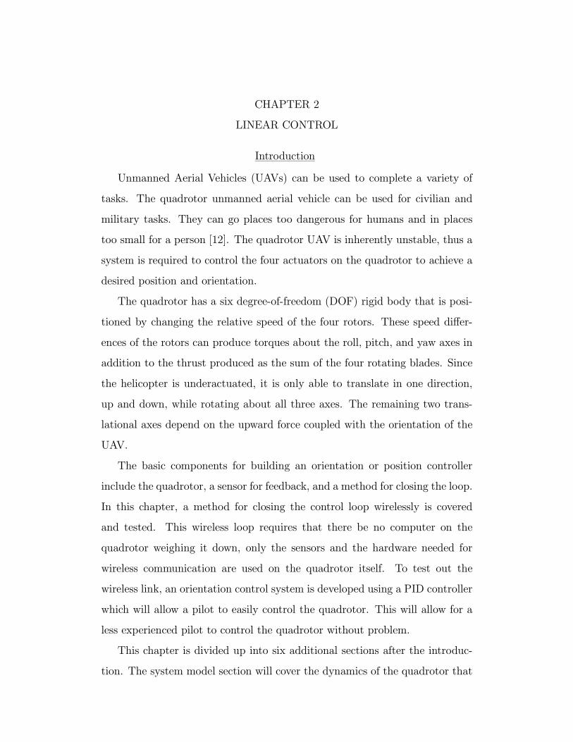
This chapter is divided up into six additional sections after the introduc-
tion. The system model section will cover the dynamics of the quadrotor that
zf
(yaw)
(front)
xf
(roll)
yf
(pitch)
UAV
Figure 2.1 Yaw, pitch, and roll definitions.
will be used in the simulations, as well as the kinematics and coupling effect
of the quadrotor design. The control method section will cover how these sen-
sors will be used in a PID system to control the quadrotor. Simulation and
implementation will cover the software used for the simulation and controller
and implementing it on the DraganFlyer X-Pro quadrotor helicopter. Obser-
vations and results will cover how well the controller works followed by the
conclusion.
System Model
DraganFlyer Quadrotor Overview
Figure 2.2 displays the different effects of certain rotor combinations. The
depiction in Figure 2.2.a shows all four rotors spinning at an equal rate which
results in an upward force in the z-direction. Since the rotors on the Dra-
ganFlyer X-Pro can only spin in one direction, the forces from each rotor and
the sum of all four rotors will always be added up in the negative z-direction,
according to Figure 2.1. If all the rotors spin faster then the craft will rise and
if all spin slower then the craft will settle.
The intriguing aspect of a quadrotor is the manner in which the torques,
that can be used to move the quadrotor, are generated. The four rotors can
6
be grouped into two sets, group A consisting of the front and back rotors
and group B consisting of the left and right rotors. Both rotors in group A
spin counter-clockwise while both rotors in group B spin clockwise, shown in
Figure 2.2. Pitch will be defined as rotation about the y-axis, roll as rotation
about the x-axis and yaw as rotation about the z-axis, as seen in Figure 2.1.
To achieve pitch torque, the front and back rotors in group A must spin at
different speeds. To pitch clockwise, the front rotor speed is decreased and
the rear rotor speed increased while keeping the left and right rotors in group
B constant, as depicted in Figure 2.2.b. The front rotor is increased and
the back rotor is equally decreased so that the total sum of the four rotor
forces remain the same. The same method is used for generating a roll torque
in the clockwise direction as seen in Figure 2.2.c. The third body torque is
applied using a different method; instead of using the thrusting forces of the
rotors as done for roll and pitch, rotating in the yaw direction uses torque
couples. Since group A spins counter-clockwise and group B spins clockwise,
the quadrotor creates a clockwise couple and counter-clockwise couple. When
all four rotors spin at the same speed, the couples cancel out and there is no
yaw rotation. But when group B slows down, and group A speeds up, there
will be a counterclockwise rotation as illustrated in Figure 2.2.d.
The DraganFlyer X-Pro is designed for each rotor to spin in one direction
only. Because of this restriction, there are certain situations in which all
torques cannot be arbitrarily applied. The first example in Figure 2.3.a is
when all four rotors are stopped. If roll is the desired torque, one motor
cannot be decreased while the opposite is increased as an undesired yaw force
will be introduced. This yaw force can be cancelled out with the other two
rotors, but then an undesired upward force is generated. If the motors could
spin backwards, then the roll torque could be achieved by simply spinning the
left rotor and right rotor in opposite directions. It is rare to have all four rotors
stopped while flying. The example in Figure 2.3.b is far more likely. When
trying to achieve a large yaw torque, two of the motors will shut off, making
7
Max spin
…
Medium
…
Slow
No Spin
Legend
Front
a - hovering b – pitching forward
c – rolling left d – yawing
counterclockwise
Back
A A
A A
B
B
B
B
A A
A A
B
B
B
B
Figure 2.2 Quadrotor method of applying torques to produce motion.
8
Max spin
…
Medium
…
Slow
No Spin
Legend
Front
a – undesired yaw and
thrust from roll or pitch
b – week roll while
yawing
c – week pitch while
yawing
Back
A A
A A
B
B
B
B
A
A
B
B
Figure 2.3 Peculiarities resulting from mono-directional rotor motors andblades.
9
a b c zf
xf yf
Thrust Thrust
Figure 2.4 Series of motions the quadrotor executes while moving
roll impossible or extremely weak. In order to apply a roll torque, speeding
up the left rotor only will start creating a stray yaw torque in addition to
an additional upward force. The same is true for pitch in Figure 2.3.c. One
method to prevent such a situation is to set a minimum rotor speed. That
way the quadrotor can still apply at least a small amount of torque in the roll,
pitch, and yaw directions without introducing undesired forces and torques.
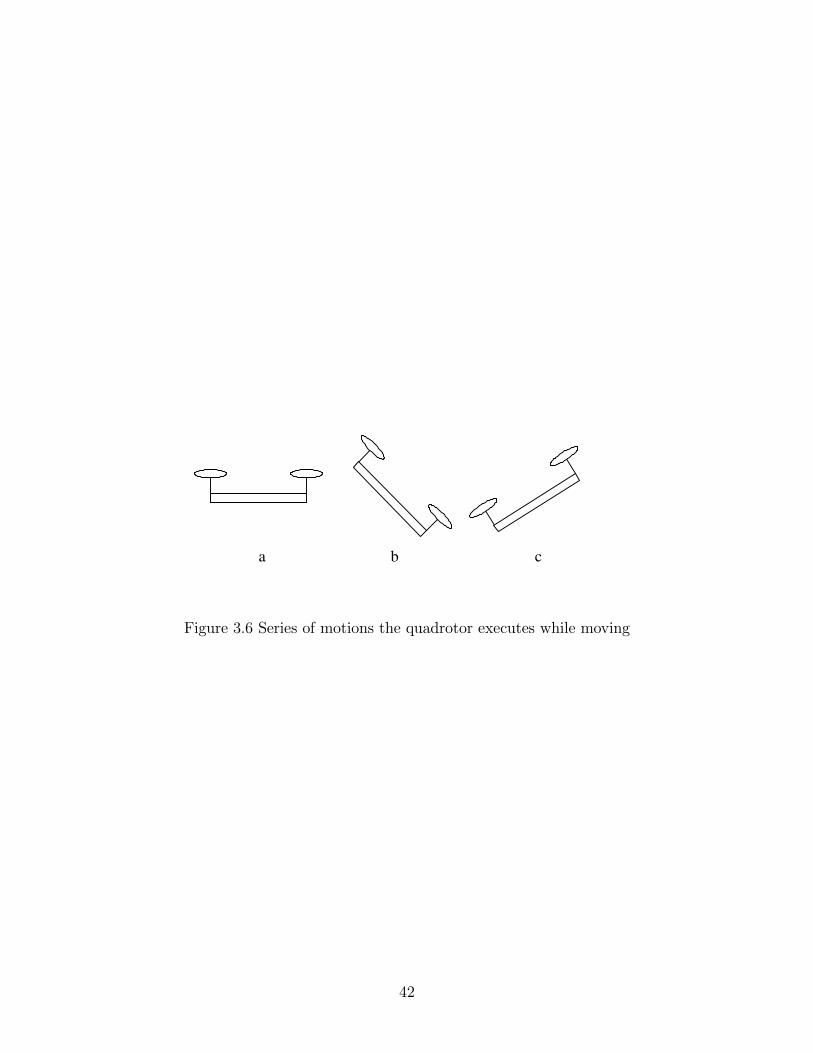
As stated, the quadrotor is underactuated, although it is still free to move
in all of its six degrees-of-freedom (DOF). An example of quadrotor motion is
shown in Figure 2.4. In Figure 2.4.a, the quadrotor is hovering. To move in
the x-direction, the quadrotor must pitch clockwise to direct a component of
the forward direction as seen in Figure 2.4.b. To come to a stop, the quadrotor
must pitch back as seen in Figure 2.4.c to bring the quadrotor’s velocity down
to zero. Once the quadrotor horizontal motion has stopped, it returns to the
horizontal state, Figure 2.4.a. This is the coupling between the pitch angle
and the x-direction which is used to move in the forward direction. The same
coupling is seen between the roll angle and the y-direction. Note that the
rotor speeds must increase in Figures 2.4.b and 2.4.c above Figure 2.4.b as the
thrust component that counters gravity is reduced.
Quadrotor Dynamics Model
As discussed above, the quadrotor UAV, such as the DraganFlyer X-Pro
quadrotor [18], is an inherently underactuated system. While the angular
10
zi
xi
yi
Inertial
(I)
zf
xf
yf
U AV
(F)
I
I F
I
F
x
R
Figure 2.5 The quadrotor helicopter coordinate frames
torques are directly actuated, the translational forces are only directly actuated
in the z-direction. The forces and torques are expressed as
F Ff =
[0 0 u1
]ᵀ ∈ R3F Ft =
[u2 u3 u4
]ᵀ ∈ R3 (2.1)
where F Ff (t) refers to the UAV translational forces expressed in the UAV frame
F and F Ft (t) are the UAV torques expressed in the UAV frame, as seen in
Figure 2.5.
Rigid body dynamics are used for the UAV dynamics because the quadrotor
is a rigid body that can thrust and torque freely in space. The four equations
to describe the UAV’s rigid body dynamics are [3] in
xIIF = RIFv
FIF (2.2)
mvFIF = −mS(ωFIF
)vFIF + N1 (·) + mgRF
I e3 + F Ff (2.3)
RIF = RI
FS(ωFIF
)(2.4)
MωFIF = −S(ωFIF
)MωFIF + N2 (·) + F F
t (2.5)
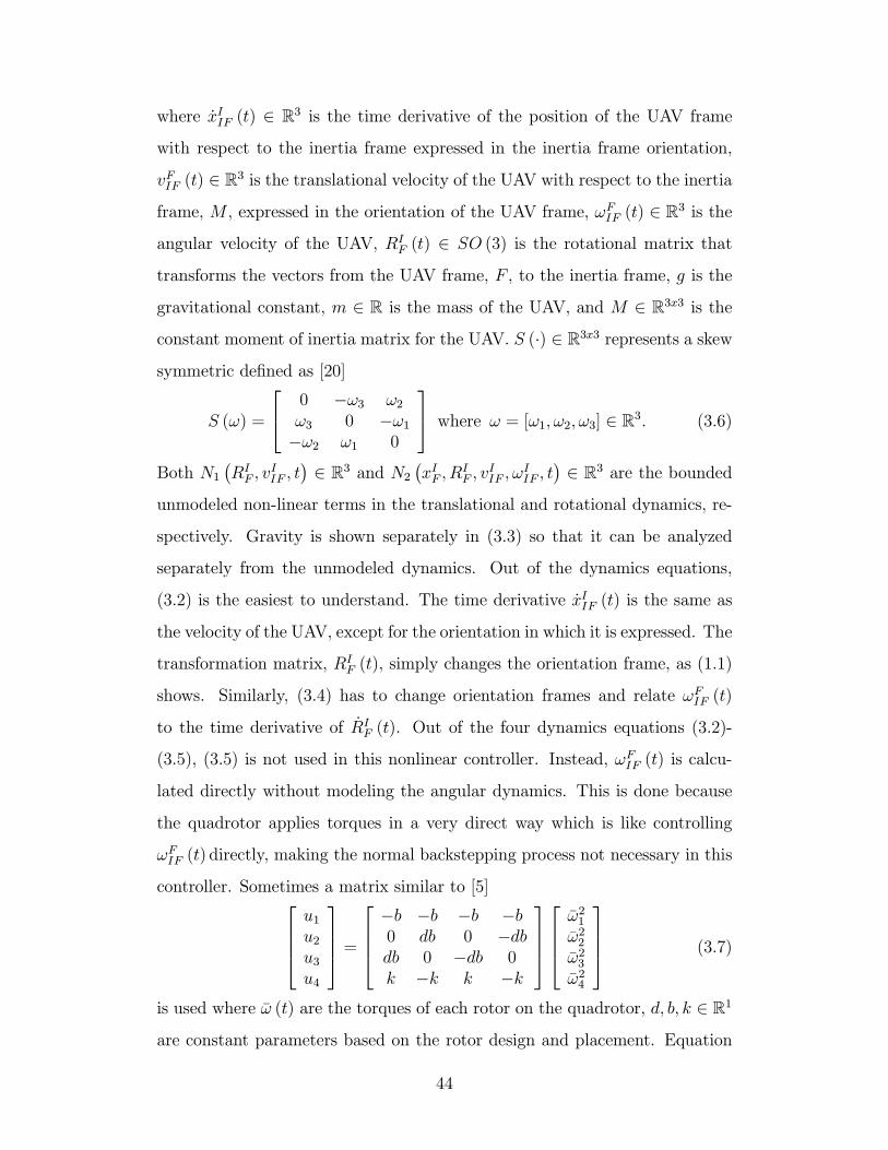
where xIIF (t) ∈ R3 is the time derivative of the position of the UAV frame
with respect to the inertia frame expressed in the inertia frame orientation,
11
vFIF (t) ∈ R3 is the translational velocity of the UAV with respect to the inertia
frame, M , expressed in the orientation of the UAV frame, ωFIF (t) ∈ R3 is the
angular velocity of the UAV, RIF (t) ∈ SO (3) is the rotational matrix that
transforms the vectors from the UAV frame, F , to the inertia frame, g is the
gravitational constant, m ∈ R is the mass of the UAV, and M ∈ R3x3 is the
constant moment of inertia matrix for the UAV. S (·) ∈ R3x3 represents a skew
symmetric defined as [20]
S (ω) =
0 −ω3 ω2ω3 0 −ω1−ω2 ω1 0
where ω = [ω1, ω2, ω3]ᵀ ∈ R3. (2.6)
Both N1
(xIF , R
IF , v
IIF , ω
IIF , t
)∈ R3 and N2
(xIF , R
IF , v
IIF , ω
IIF , t
)∈ R3 are the
unmodeled non-linear terms in the translational and rotational dynamics, re-
spectively. Gravity is shown separately in (2.3) so that it can be analyzed
separately from the unmodeled dynamics. Out of the dynamics equations,
(2.2) is the easiest to understand. The time derivative xIIF (t) is the same as
the velocity of the UAV, except for the orientation in which it is expressed.
The transformation matrix, RIF (t), simply changes the orientation frame, as
(1.1) shows. Similarly, (2.4) has to change orientation frames and relate ωFIF (t)
to the time derivative of RIF (t). Sometimes a matrix similar to [5]
u1u2u3u4
=
−b −b −b −b0 db 0 −dbdb 0 −db 0k −k k −k
ω21ω22ω23ω24
(2.7)
is used where ω (t) are the torques of each rotor on the quadrotor, and d, b, k ∈R1 are constant parameters based on the rotor design and placement. Equation
(2.7) describes the relationship between the four rotor torques on the quadrotor
and the forces and torques of the quadrotor from (2.1). With the DraganFlyer
X-Pro (and most quadrotor RC helicopters) this calculation is done internally
and the joystick inputs are mapped to u (t) instead of ω (t).
12
Quadrotor Kinematic Model
Many of the equations, such as (2.2)-(2.4), will need either RIF (t) or RF
I (t).
While (2.4) expresses how to get RIF (t), it involves integrating an SO (3) ma-
trix, which will not yield another SO (3) matrix due to numerical integration
method errors. However, the integration can be done on the roll, pitch, and
yaw angles. A Jacobian will be required in order to satisfy the equation
ωFIF = JF ΘFIF (2.8)
which can then be used to solve for
ΘIF =
∫ t
0
J−1F ωFIFdt (2.9)
where ΘIF (t) ∈ R3 represents the roll, pitch, and yaw angles between the UAV
frame and inertia frame. The Jacobian matrix used, J−1F(ΘIF (t)
)is defined as
[2]
J−1F =
1 sinψ tan θ cosψ tan θ0 cosψ − sinψ0 sinψ/ cos θ cosψ/ cos θ
, ΘIT =
ψθφ
. (2.10)
As long as the θ term is not near ±π2, the yaw, pitch, roll representation will
not reach singularity. To convert between RIF (t) and ΘI
F (t),
RIF =
cosφ cos θ − sinφ cosψ + cosφ sin θ sinψsinφ cos θ cosφ cosψ + sinφ sin θ sinψ− sin θ cos θ sinψ
(2.11)
sinφ sinψ + cosφ sin θ cosψ− cos φ sinψ + sinφ sin θ cos φ
cos θ cosψ
is used [20].
Control Method
Because of the coupling explained in the previous sections, it was decided to
make the system control the pitch and roll angles at the expense of controlling
the x and y position directly. By controlling these angles, commanding the
quadrotor to move forward will be the same as commanding the quadrotor to
13
pitch forward in the pattern displayed in Figure 2.4. Since the yaw angle is
not coupled with a direction, it can rotate without affecting the position and
the yaw velocity which will facilitate the design of a controller that will allow
for the user to command the quadrotor to rotate the yaw at a certain rate
instead of to a certain angle.
Since the quadrotor UAV controls its torques directly, it is easier to control
the angle. Using a proportional-derivative-integral (PID) controller, the non-
linearities from (2.4) and (2.5), primarily the S(ωFIF
)MωFIF and the unmodeled
non-linearities N2 (·), will be ignored. By using the torque F Ft (t) as a control
signal, a feedback system can be developed based on
u = −kpe− kdde
dt− ki
∫e (2.12)
where u (t) is the control signal, e (t) is the error signal, kp is the proportional
gain, kd is the differential gain, and ki is the integral gain. The error signal
used, eθ (t) ∈ R3, consists of
eroll = θroll − θrolld (2.13)
epitch = θpitch − θpitchd (2.14)
eyaw = θyaw − θyawd (2.15)
where θyawd (t) is
θyawd =
∫θyawd. (2.16)
Based upon these signals, the feedback signals used are
u1 = u1 (2.17)
u2 = −kp rolleroll − kd roll
depitchdt
− ki roll
∫eroll (2.18)
u3 = −kp pitchepitch − kd pitch
depitchdt
− ki pitch
∫epitch (2.19)
u4 = −kp yaweyaw − kd yaw
deyawdt
− ki yaw
∫eyaw. (2.20)
The desired trajectories that will be generated will create the values for u1 (t),
θrolld (t), θpitchd (t), and θyawd (t).
14
This approach takes a PID linear approach and applies it to the non-linear
system. It is not known if the non-linearities cause any significant instabilities,
however the goal of this was to verify the wireless closed looped system will
work.
Simulation and Implementation
Quadrotor Model Simulation Parameters
In order to have an accurate simulation of the DraganFlyer X-Pro, certain
parameters have to be measured. The mass and inertia matrix are needed for
the dynamics equations and the actual maximum thrust and torques produced
by the quadrotor are needed to set realistic limits on the simulation.
To measure the mass, the helicopter was weighted using a spring scale. To
measure the total force the helicopter can produce, a spring scale is used to
measure the amount of force one rotor can create when spinning at maximum
speed. This quantity multiplied by four will yield the full thrust ability. In
addition, the distance from the rotor to the center of the UAV will yield the
total roll and pitch torque that can be generated with one rotor spinning at
its maximum velocity while the opposite rotor stopped, as in Figure 2.2.b.
A similar measurement was made when two opposite rotors were spinning
at maximum speed and the other two rotors were off, as in Figure 2.3.b, to
estimate the maximum yaw torque. All of these measurements are displayed
in Table 2.1. The inertia matrix was not measured and was estimated based
off of [9][7] where the vehicle was half the weight of the DraganFlyer, so the
values of the inertia matrix were doubled to
M =
1.3 0 00 1.3 00 0 2
kg ·m2. (2.21)
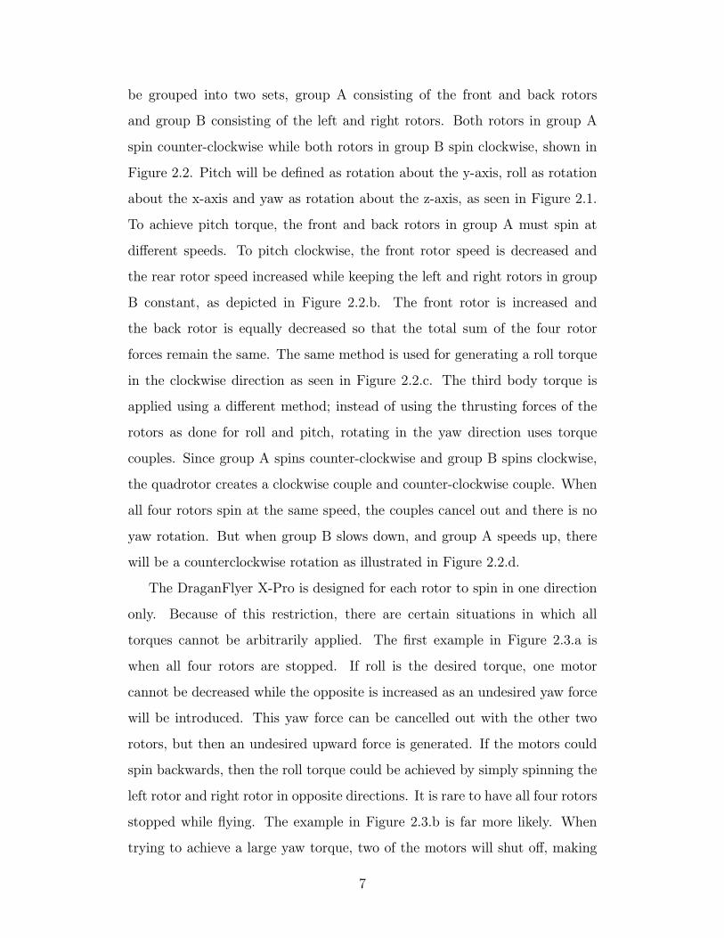
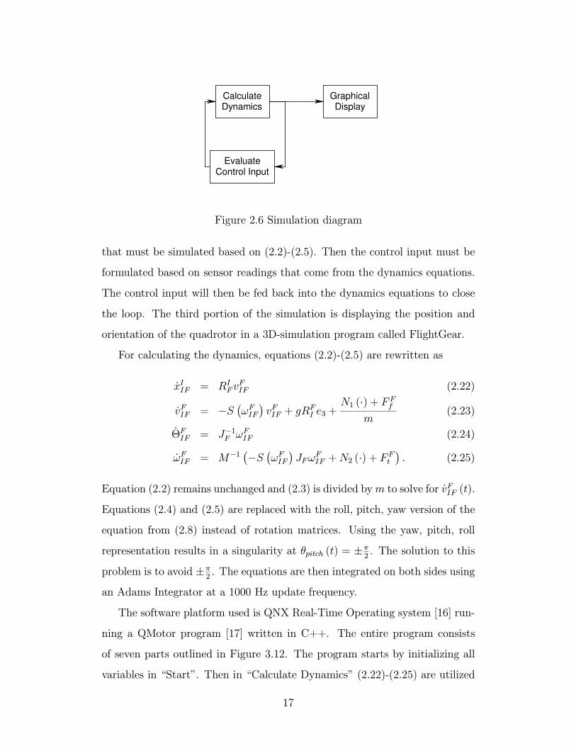
Simulation
To simulate this controller, there are three main tasks that must be im-
plemented as seen in Figure 2.6. The first block is the helicopter dynamics
15
Table 2.1 DraganFlyer X-Pro Parameters
Parameter Value UnitsMass 2.041 kgAdditional Weight (battery and sensors) .68 kgMax Thrust 35.586 NMax Roll Torque 4.067 NmMax Pitch Torque 4.067 NmMax Yaw Torque 2.034 Nm
16
CalculateDynamics
GraphicalDisplay
EvaluateControl Input
Figure 2.6 Simulation diagram
that must be simulated based on (2.2)-(2.5). Then the control input must be
formulated based on sensor readings that come from the dynamics equations.
The control input will then be fed back into the dynamics equations to close
the loop. The third portion of the simulation is displaying the position and
orientation of the quadrotor in a 3D-simulation program called FlightGear.
For calculating the dynamics, equations (2.2)-(2.5) are rewritten as
xIIF = RIFv
FIF (2.22)
vFIF = −S(ωFIF
)vFIF + gRF
I e3 +N1 (·) + F F
f
m(2.23)
ΘFIF = J−1F ωFIF (2.24)
ωFIF = M−1(−S
(ωFIF
)JFω
FIF + N2 (·) + FF
t
). (2.25)
Equation (2.2) remains unchanged and (2.3) is divided by m to solve for vFIF (t).
Equations (2.4) and (2.5) are replaced with the roll, pitch, yaw version of the
equation from (2.8) instead of rotation matrices. Using the yaw, pitch, roll
representation results in a singularity at θpitch (t) = ±π2. The solution to this
problem is to avoid ±π2. The equations are then integrated on both sides using
an Adams Integrator at a 1000 Hz update frequency.
The software platform used is QNX Real-Time Operating system [16] run-
ning a QMotor program [17] written in C++. The entire program consists
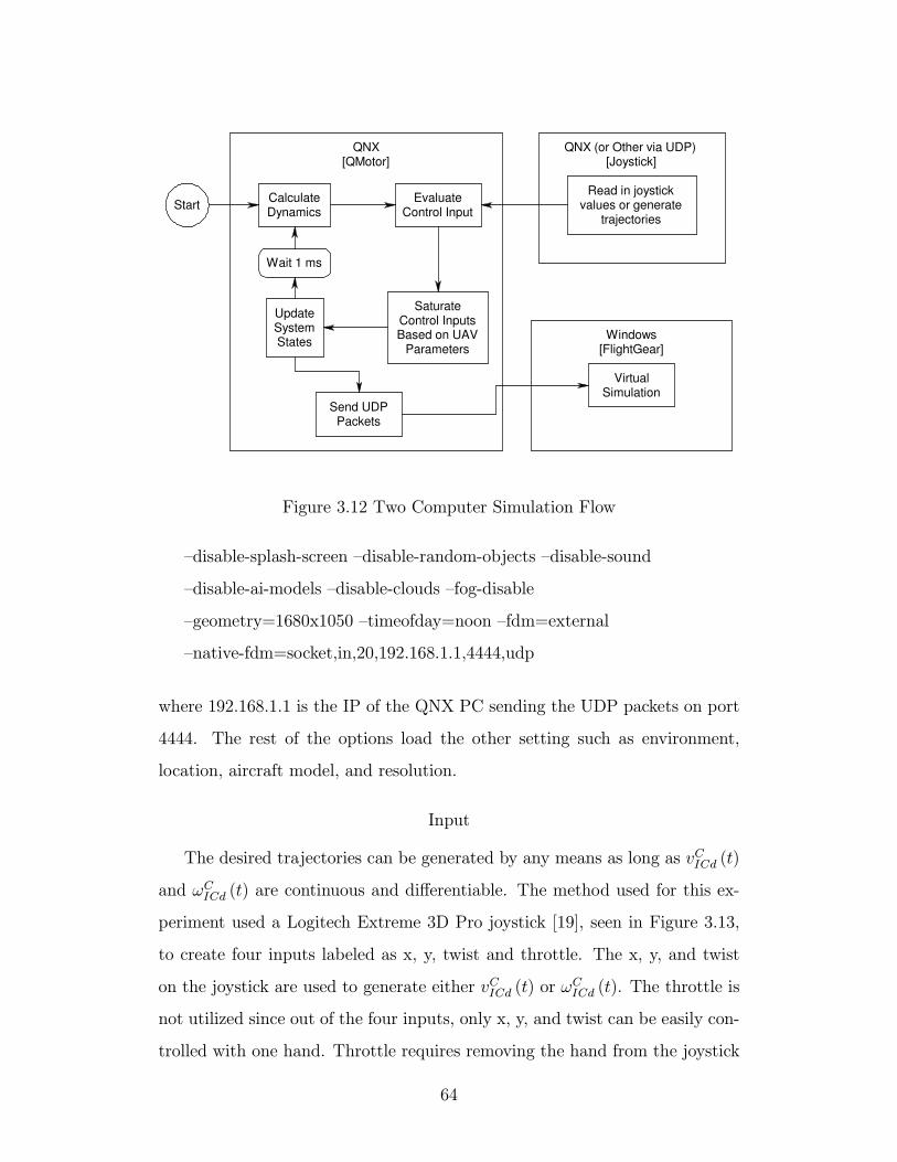
of seven parts outlined in Figure 3.12. The program starts by initializing all
variables in “Start”. Then in “Calculate Dynamics” (2.22)-(2.25) are utilized
17
to find xIIF (t), vFIF (t), ΘIF (t), and ωFIF (t). In “Evaluate Control Input” the
program uses the trajectories for θrolld (t), θpitchd (t), θyawd (t), and u1 from
“Read in joystick values and generate trajectories” to evaluate (2.17)-(2.20).
“Saturate Control Inputs Based on UAV Parameters” uses the parameters
from Table 2.1 to make sure the control inputs do not exceed realistic values,
and if they do, it saturates the value to the maximum limits. A minimum
rotor speed is also utilized to prevent the quadrotor coupling peculiarities due
to the motors only spinning in one direction. Not only are the singularities
prevented, but the effects of the coupling between the different torques are also
included in the control inputs. “Update System States” is where all the posi-
tions and velocities in the inertia, UAV, and camera frames are computed for
use in other calculations in the next iteration. The resulting position and ve-
locity are sent to FlightGear by “Send UDP Packets” and received and shown
on the screen by “Virtual Simulation.” The code for the QNX program can
be found at http://www.ece.clemson.edu/crb/research/uav/simulation.zip. In
the simulate.cpp file, the “Send UDP Packets” is accomplished by
d flight UDP->PackitSend(Latitude, Longitude, Altitute, Roll, P itch, Y aw);
where all numbers are in radians except altitude which is in meters and
d flight UDP is of type FlightUDP. A UDP is send to a PC on a specific
port defined in the constructor in FlightUDP.cpp as
d UDP client=new UDPClient(“192.168.1.100”,4444,d timeout);
where the UDP packet is sent to the FlightGear IP address, 192.168.1.100 in
this case, on port 4444 and d timeout is a struct of type timeval set to 50ms.
The UDP packet is of type FGNetFDM defined by net fdm.hxx [1]. The only
use for the second computer is the FlightGear simulation, because a simulation
such as FlightGear requires| almost all of a computer’s CPU, video card, and
input/output system [1]. To execute the FlightGear simulator at GSP airport,
where 192.168.1.1 is the IP of the QNX PC sending the UDP packets on port
4444. The rest of the options load the other setting such as environment,
location, aircraft model, and resolution.
Input
The desired trajectories can be generated by any means as long as vCICd (t)
and ωCICd (t) are continuous and differentiable. The method used for this ex-
periment used a Logitech Extreme 3D Pro joystick [19], seen in Figure 3.13,
to create four inputs labeled as x, y, twist and throttle. The x, y, and twist
on the joystick are used to generate either vCICd (t) or ωCICd (t). The throttle is
not utilized since out of the four inputs, only x, y, and twist can be easily con-
trolled with one hand. Throttle requires removing the hand from the joystick
64
x
y
Twist
Throttle
Figure 3.13 Logitech Wingman Extreme 3D Pro joystick
or using a second hand. One method of using this joystick is to only input
three of the desired velocities at one time. Depending on whether Button 1
is pressed, the joystick’s three axes will control the 3 translational velocities,
vCICd (t), or the three angular velocities, ωCICd (t). However this prevents all six
degrees from being controlled at once. A second method uses two Wingman
joysticks to allow the user to control three desired velocities with each hand,
for a total of all six desired velocities.
FlightGear
FlightGear is an open-source flight simulator [1]. It can run on many com-
puter platforms including Linux and Windows. FlightGear offers a versatile
package with multiple input-output (I/O) systems and an interface for import-
ing custom helicopter models. FlightGear is used to display the position and
65
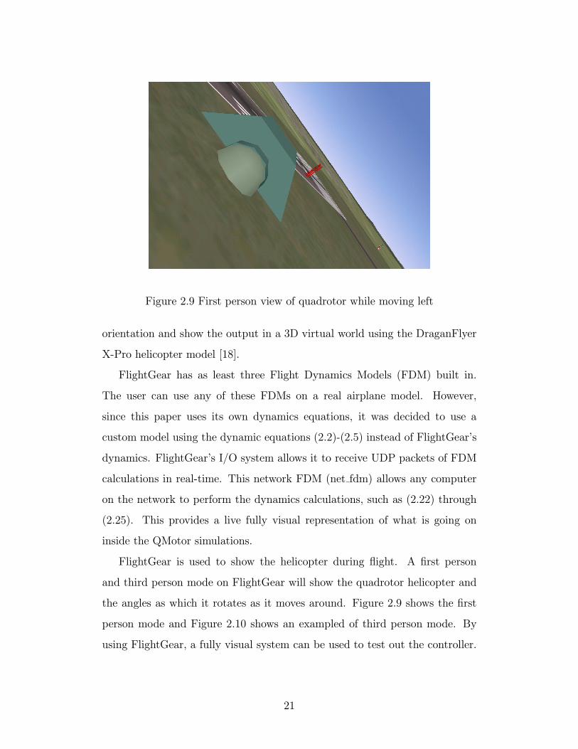
orientation and show the output in a 3D virtual world using the DraganFlyer
X-Pro helicopter model [18].
FlightGear has as least three Flight Dynamics Models (FDM) built in.
The user can use any of these FDMs on a real airplane model. However,
since this paper uses its own dynamics equations, it was decided to use a
custom model using the dynamic equations (3.2)-(3.5) instead of FlightGear’s
dynamics. FlightGear’s I/O system allows it to receive UDP packets of FDM
calculations in real-time. This network FDM (netfdm) allows any computer
on the network to perform the dynamics calculations, such as (3.2) through
(3.5). This provides a live fully visual representation of what is going on inside
the QMotor simulations.
There are two useful viewpoints that can be shown from FlightGear. The
most important of these is the camera view. Since this is a fly-by-camera inter-
face, it is useful to be able to see the camera view for simulation. FlightGear’s
first person view looks out the quadrotor’s x-axis, as seen in Figure 3.8. To
accomplish this, a transformation is made so that the camera frame’s z-axis is
the x-axis seen in the simulator using the rotation matrix
RsimulationC(fonrt) =
0 0 −10 1 01 0 0
(3.86)
that goes from the camera frame to the FlightGear simulation frame. If the
camera were mounted on the bottom of the helicopter as seen in Figure 3.9, the
transformation will be from the camera’s z-axis to the z-axis on the helicopter.
This transformation is needed because FlightGear is attempting to display
the UAV and this transformation allows it to display the camera correctly,
allowing for a complete camera view in the simulator. The other important
camera view is the helicopter itself. A third person mode on FlightGear will
show the quadrotor helicopter and the angles as which it rotates as it moves
around. QMotor has the option of showing either the camera frame for first
person mode or the UAV frame for third person mode to demonstrate what
the helicopter is actually doing.
66
Figure 3.14 First person view of quadrotor while moving left
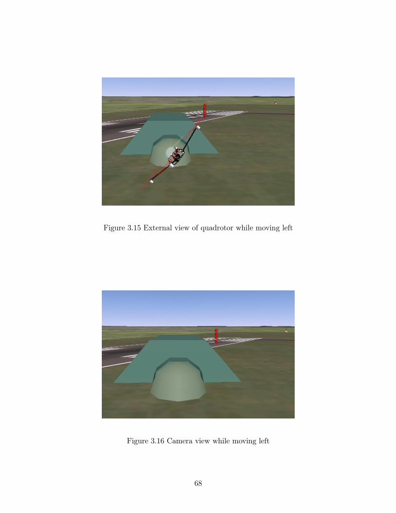
FlightGear is used to show two points of view while the simulation is run-
ning: the UAV view and the camera view. The UAV view will show the
position and orientation of the UAV helicopter. Likewise, the camera frame
shows the orientation and position of the camera. It is important to show the
camera for the simulation since the experiment is the fly by camera interface.
In Figures 3.14 and 3.15, the UAV is oriented so that it can move to the left.
Figure 3.16 shows what the camera will show in the same situation. The actual
level of the ground can be seen in Figure 3.15 and is approximately the same
in Figure 3.16, thus demonstrating the independence of the UAV and camera
frame.
Observations and Results
The very first simulations were a complete failure. This is because the
original U1 control input was different from (3.52). Instead, U1 was defined as
U1 = −krrv − rvζ21(∥∥vFIF
∥∥)
ε1+ S
(ωCIC
)vCICd (3.87)
with no G11 (t) term and the ev (t) replaced by rv (t). The lack of a G11 (t)
term was because it was originally intended that gravity would be included
67
Figure 3.15 External view of quadrotor while moving left
Figure 3.16 Camera view while moving left
68
in the N11 (t) term. This was extremely difficult to overcome because accord-
ing to Table 3.3 the DraganFlyer X-Pro uses approximately 75% of it’s total
thrust just to overcome gravity. Using rv (t) instead of ev (t) also proved to be
unusable. Using (3.26), (3.87) can be rewritten as
U1 = −krev − krRCF δ − rv
ζ21(∥∥vFIF
∥∥)
ε1+ S
(ωCIC
)vCICd. (3.88)
The krRCF δ term was adding a constant to the control input, and overpowering
the rest of the system making it unusable. This is where the solution of using
(3.52) came from. (3.87) satisfies its own Lyapunov proof and the velocities
were GUUB, however they never came near to zero and the bound could not
be made arbitrarily small on ev (t).
In simulation when the UAV is just hovering, it will stand still with no
errors using (3.52) and (3.59). To examine how the control reacts, a simple
experiment is conducted by commanding the camera to move left and right.
All of the experiments are conducted with δ = 100, kr = 1, and no ki because
there is no angular error in the simulation. To look at how the velocities and
positions of the camera react, the first experiment will show the UAV going left
then right using the first camera mounting method highlighted in Figure 3.8.
The desired velocity graph seen in Figure 3.17 is used on the y-coordinate of
the camera frame only. All values remain zero for the first 15 seconds of the
experiment and are not shown. The desired x- and z-velocities remain zero and
ωCICd = 0. The actual velocities of the camera frame in Figure 3.20 approach
the desired velocities in a few seconds. It can also be seen that the x-velocity
changes when the camera moves left and right. This is because gravity is in
the x-direction. Sudden changes cause the quadrotor to lift or fall a little,
however, the controller does respond and stabilizes the x velocity to zero.
In this first experiment when the camera is commanded to go left and right,
the UAV will tilt left and right along the camera z-axis, as seen in Figure 3.18.
The other two axes not shown remain zero for the entire simulation. The graph
shows the UAV tilting over .5 radians (29 degrees). The controller is suppose
69
Figure 3.17 Desired velocities of Camera Frame (vCICd ): Experiment 1
70
to apply a counter rotation to the camera frame in an attempt to minimize
the amount of rotation felt in the camera frame. As seen in Figure 3.19, the
camera frame’s rotation is much less than that of the UAV. There is still a
certain amount of rotation error in the camera frame. However, the error is not
due to an error in ωCIC (t). In the simulation, eω (t) is zero since the simulation
model controls the angular rates directly. The error is caused by the design of
the controller. The error is in the rotation of the camera, however the feedback
and inputs are in terms of angular velocities. Because the exact angles of the
UAV and camera are not known by the controller, there is a drifting error in
the camera rotation. The camera angles are essentially a result of integrating
the control inputs, thus creating this drift error over time. The drift error in
the translational velocities is less detrimental because the position error is not
focused on.
The camera is tilting a little more in the opposite direction than needed.
When the UAV turns left .38 radians, the camera is actually turning right
.46 radians, resulting in the final .08 radian rotation. This gives viewers and
observers a counterintuitive feeling because they are familiar with there being
no correction.
The error is relatively small and is easy to compensate for by telling the
camera to tilt a little in the opposite direction of the error. The total error
after about a minute of flight time can be seen in Figures 3.18 and 3.19 when
the UAV angle returns to zero and the camera angle settles around .15 radi-
ans (8.6◦). The feel from the camera is a lot smoother then if there was no
correction.
If the drift error seen in Figure 3.19 is to be fixed, then the controller has to
be changed. Theorem 1 does not state that the angles are bounded. In order
to control the angles, an angle sensor will need to be added to the controller.
With angle feedback, the angle can be controlled and the error can eventually
be bounded.
In this particular experiment, the desired camera angle was zero throughout
71
Figure 3.18 Angles of UAV while moving left and right (ΘFI )
Figure 3.19 Camera error while moving left and right (ΘCI )
72
the experiment, even though the actual angle is not zero as seen in Figure 3.19.
Because of this, the velocities expressed in the camera frame and the inertia
frame are in fact different. It is interesting to compare these velocities to
evaluate how significant this error is. In Figure 3.20, the camera y velocity can
be seen to be in the approximate shape of the desired velocity in Figure 3.17.
There is an apparent flat spot around 25 second and 35 seconds. While the
z-velocity remains zero the entire experiment, the x-velocity does not. This
is because the x-velocity is along the same axis as gravity in the Figure 3.8
configuration. When the quadrotor rolls left and right, rotation about the
x-axis is disturbed and the controller must correct for this. As stated before,
if there were no errors in the rotation, then vCIC = vC(0)IC , where C (0) is the
camera frame at time 0. Comparing Figure 3.20 to Figure 3.21, there are
small differences, however the errors seen in Figure 3.19 do not make a huge
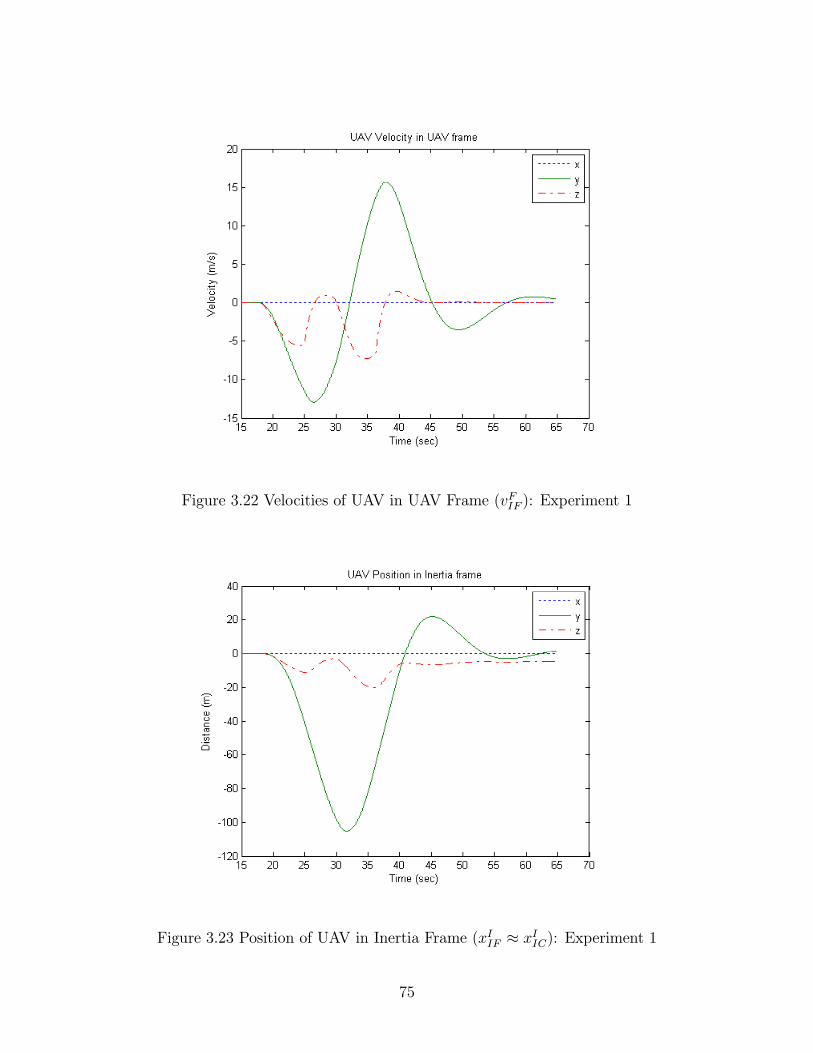
difference in the velocities. The last velocity to look at is the UAV velocity in
the UAV frame seen in Figure 3.22. It is a much smoother curve compared to
the rest. This is how the quadrotor actually reacts: in smooth glides left and
right.
Another interesting graph to look at is the path the UAV and camera
actually travel in. Since the camera is closely mounted onto the UAV, it is
safe to say their positions are approximately the same. Figure 3.23 shows the
y-position going left then coming back right. Since the velocity to the right
seen in Figure 3.21 is faster and longer then to the left, the UAV ends up
going right more, before settling close to zero. The z-position is off by about
5 meters in the end. This is all part of the drift error that will occur in the
position when only the velocity is bounded, as stated in Theorem 1.
Examining the control inputs for the first experiment shows that the FFf
control input u1, seen in Figure 3.24, only reaches its saturation point once,
at around 30 seconds. Due to the controller’s nature, where there are sharp
changes in the velocities, there are sharp changes in the thrusts, seen especially
at 25, 30, and 36 seconds. As for the other control inputs, only the x-axis of
73
Figure 3.20 Velocities of Camera Frame (vCIC): Experiment 1
Figure 3.21 Velocities of Camera in a Fixed Inertia Frame (vC(0)IC ):
Experiment 1
74
Figure 3.22 Velocities of UAV in UAV Frame (vFIF ): Experiment 1
Figure 3.23 Position of UAV in Inertia Frame (xIIF ≈ xIIC): Experiment 1
75
Figure 3.24 UAV trust (FFf ): Experiment 1
ωFIF and the roll angle of θC do not remain zero, as shown in Figure 3.25. It
can be seen that these two curves are near opposites of each other, as would
be expected given the desired inputs and the θC .
The exact same results are seen in a second experiment when the desired
velocities tell the camera to go forward and backward instead of left and right,
since the quadrotor is completely symmetrical in this way.
In a third experiment, the camera is commanded to go up and down to
examine the effects that a limited thrust has. ωCICd is kept at zero while vCICd
is in the shape of Figure 3.26. Since the quadrotor is only translating in the
up and down directions, there will be no torques or change of angle. The
actual velocity achieved by the camera can be seen in Figure 3.27. Since the
thrust is limited to 35.586 N in Table 3.3, the quadrotor only significantly
reaches its limit at 7 seconds and again at 40 seconds, seen in Figure 3.28.
By comparing the acceleration of the UAV in Figure 3.27, it can be seen that
the acceleration up is much slower then the acceleration down due to this
76
Figure 3.25 UAV Angular rates (ωFIF and θC): Experiement 1
77
Figure 3.26 Desired velocities of Camera Frame (vCICd ): Experiment 3
limitation. The saturation points reached at 15 seconds and 31 seconds are
there to stop the rotors from spinning and losing all roll, pitch, yaw control.
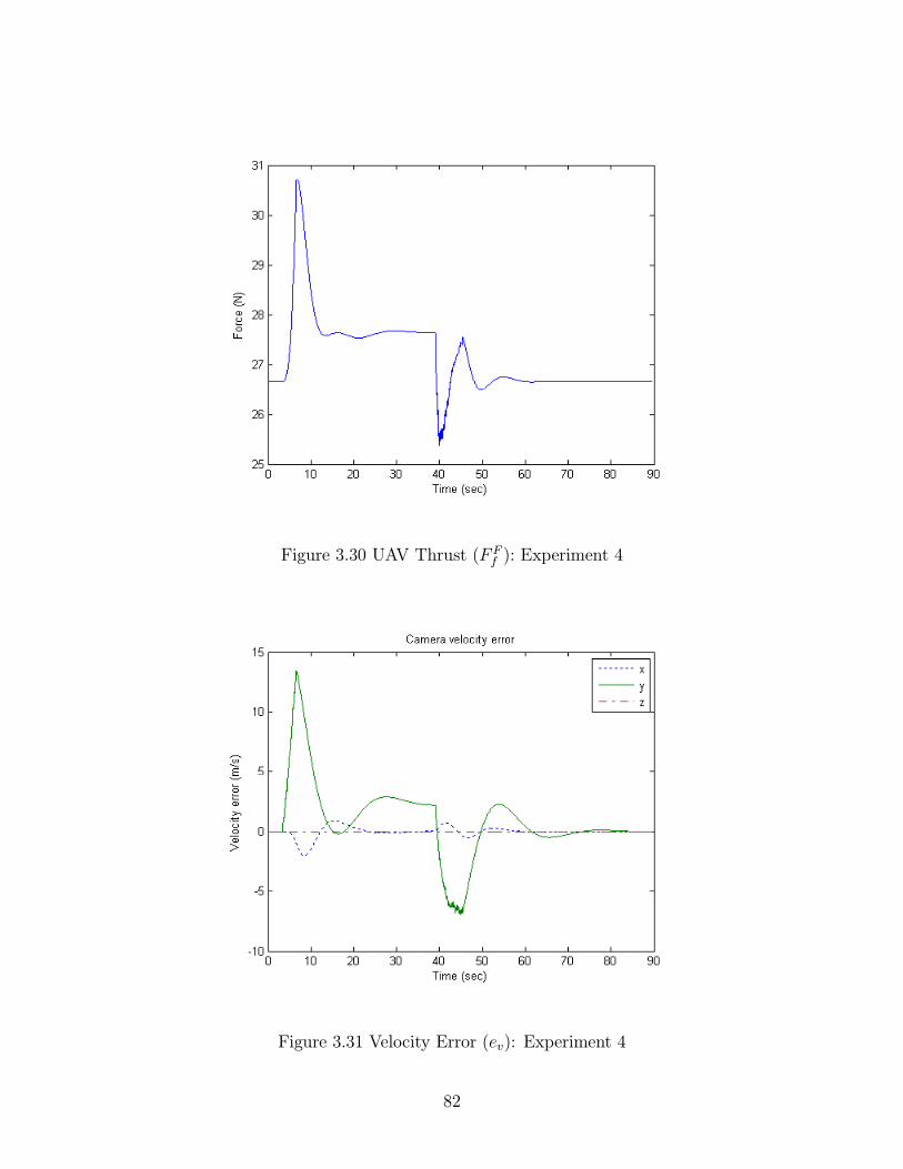
In the last experiment, a smoother desired velocity is used to tell the
quadrotor to move right then stop, as seen in Figure 3.29. Looking at the
camera velocities, it can be seen that there is a small overshoot at around
15 seconds, and then the velocity settles near the desired 15 m/s. The same
event occurs at around 50 seconds as the quadrotor comes to a stop. Similar
to experiment 1, the UAV drops in the camera’s x-direction. The drop in the
x-direction is smaller then that observed in experiment 1. In addition, a small
angular error can be observed. However this error is less then .1 radians for
all time, smaller than that from experiment 1. With less sudden changes in
the desired velocity, there is less error in the angles of rotation and less of a
drop in the x-direction. The thrust control input F Ff in Figure 3.30 varies con-
siderably less than experiment 1 did. The velocity error shown in Figure 3.31
shows most of the error in the y-direction and is in the same shape as u1 seen
78
Figure 3.27 Velocities of Camera Frame (vCIC): Experiment 3
Figure 3.28 UAV trust (FFf ): Experiment 3
79
in Figure 3.30. All of these results are expected for this kind of experiment.
All of these experiments show that the controller is GUUB in both vCIC
and ωCIC . One of the difficulties in a velocity controller like this is that the
positions and angles are not bounded and can only be kept small by making
the bounds on the velocities close to zero. By using (3.52) instead of (3.87),
it is possible to have a useful velocity GUUB controller.
Future Work
There are a number of improvements that can be made on this controller
for the future. One improvement would be to add a kvi integral gain into
equation (3.52) to make
U1 = −krev − rvζ21(∥∥vFIF
∥∥)
ε1+ S
(ωCIC
)vCICd − kviei −G11 (3.89)
where
ei � RIC
∫vCIC − vCICd. (3.90)
This will help compensate for constant errors and is especially good for cor-
recting for uncertainties in gravity. This relaxes the restriction that gravity
to be known. It has been observed that small uncertainties in gravity will
cause the velocities to drift to an offset instead of going to zero, as would
be expected. Another improvement to (3.52) could be to use a predictor for
vCICd (t). By adding a ‖rv‖∥∥vCICd
∥∥ term to U1 to get
U1 = −krev − rvζ21(∥∥vFIF
∥∥)
ε1+ S
(ωCIC
)vCICd − ‖rv‖
∥∥vCICd∥∥−G11, (3.91)
there will be no need for a β1 (t) term in (3.70). ε2 will become
ε2 = kr ‖δ‖ (3.92)
and there would be a smaller constant that does not vary with vCICd (t).
Another change that should be added is the frame in which the gains are
added. As seen in (3.90), there is a change of frame back to the UAV frame.
This is important because the kiei term will be used to remove slowly varying
80
Figure 3.29 Graphs of vCICd, vCIC , and θCI : Experiment 4
81
Figure 3.30 UAV Thrust (F Ff ): Experiment 4
Figure 3.31 Velocity Error (ev): Experiment 4
82
errors. Errors such as wind and gravity will never vary as the UAV turns or
the camera turns, it is detrimental to make the term with respect to any from
other then an inertia frame. Another frame that should be changed is the
krev term. This term is currently in terms of the camera frame with a single
constant kr. This forces all three axes to react the same, when in fact, only
the UAV’s x- and y-axes behave the same. A solution for this is the change
(3.52) into
U1 = −diag(RFCev)kr − rv
ζ21(∥∥vFIF
∥∥)
ε1+ S
(ωCIC
)vCICd −G11, kr ∈ R3 (3.93)
allowing for three gains for each of the three axes of the UAV. diag (·) puts
the values of a vector on the diagonal in a square matrix. The same can be
done for (3.59) changing to
U2 = −diag(RFC
∫eω
)ki + ωCICd. (3.94)
This second solution allows for a gain to control the yaw angle differently from
the roll and pitch angle, since the yaw torque is weaker then the other two.
While these changes make only small improvements in the performance, none
of them would change the main concept of this controller. A change that
would significantly change the controller is using position and orientation in
the feedback loop. While this will definitely improve the performance of the
controller, it will no longer be a velocity-only controller and the choices of
sensors and their accuracies will be more limited.
Conclusion
This chapter shows the development of a non-linear controller for use on a
quadrotor helicopter and a two DOF camera to successfully create a fully actu-
ated fly-by-camera interface. The controller is shown to be Globally Uniform
Ultimately Bounded (GUUB) using only velocity information for feedback.
The fly-by-camera system allows the camera and UAV to be controlled by the
user in an intuitive manner. Simulation verifies that the controller works based
83
on the rigid body model and that the fly-by-camera system is easy for anyone
to fly.
84
APPENDICES
Appendix A
Sensors
MIDG II Interface
To get information from the MIDG II sensor, the sensor had to be connected
to a computer through a converter. To communicate with the MIDG II sen-
sor, two tasks must be completed: i) create a hardware link from the MIDG
II connector to a PC computer’s DB-9 connector, ii) convert the MIDG II
RS-422 protocol to the PC computer’s RS-232 protocol, and iii) implement
software to parse the data packets and store the information in a convenient
data structure.. Tasks (i) and (ii) requires combining a variety of devices to
complete the data link while task (iii) requires adapting the software provided
by Microbotics Inc. to work in both Windows and QNX. Once these tasks
are completed, QNX programs will have an easy and reliable interface for
retrieving sensor data.
Connecting the MIDG II to a PC has two obstacles: i) the connecting
the connector in Figure A.1 to a DB-9 on a PC and ii) converting the signal
from RS-422 to RS-232. To power the MIDG II, pins 4 and 9 of the MIDG
II connector in Figure A.1 are connected to the on-board Lithium Polymer
battery on the UAV through an RCA plug. A standard RJ-45 connector
is used to connect to the MIDG II sensor connector, using the pin layout
displayed in Table A.1 and labeled as “MIDG II to (A) RJ-45”. Then an
RJ-45 to DB-9 connector labeled as “(A) to (B)” is used to get the signals
into a DB-9 connector using the wiring shown in the second and third column
of Table A.1. Then there is a third connector labeled as “(B) to (C)” is used
to get the signals back to the RJ-45 connector used on the Serial Converter
RS422 to RS232 (SLC22232) board from Microbotics Inc [13]. This converter
will change the RS-422 signals into the RS-232 voltage and DB-9 connector
which can there be plugged in on a PC computer. There is a USB plug that
must be plugged into a computer to power the converter. This completes the
87
first path shown in Figure A.2 using the “Wired Method”. All pathways are
bi-directional allowing for configuration data to be sent back to the MIDG II
sensor, although a majority of the data is sensor information from the MIDG
II to the PC computer.
A second method for connecting the sensor a PC involves the X-Tend Serial
Wireless transceivers [14] seen in Figure A.2 using the “Wireless Method”.
Using the “(A) to (B)” connector discussed above, the MIDG II can be plugged
into an X-Tend transceiver using the RS-422 protocol.. The X-Tend transceiver
will wirelessly communicated with another transceiver that can then connect
to a computer using RS-232, removing the need for an external RS-422 to RS-
232 converter. This is the method used for actual UAV experiments, providing
a range of up to 40 miles [14].
To use the data from the MIDG II, a client/server program is written
for the MIDG II using the software provided by Microbotics to parse the
data packets into a single data structure that includes GPS position, orien-
tation, time, and everything the sensor transmits. For Windows, the data
must be saved from the serial port to a file, and then the file can be parsed
using the Microbotics program [13]. In QNX, a server program, MIDGServer,
runs in the background and receives serial data, then parses the data pack-
ets and stores them in a single shared memory location as a data struc-
ture. Then a client program running in QMotor will read the shared mem-
Table A.1 Wiring table for the MIDG II connectionst
MIDG II Signal (A) RJ-45 (B) DB-9 (C) RJ-45Pb (Not used) 1 NC NC
NC 2 NC NCRb 3 8 8
Ground 4 5 5Ra 5 2 2Ta 6 3 3
Pa (Not used) 7 NC NCTb 8 7 7
88
Figure A.1 MIDG II RS-422 Connector [13]
(A) RJ-45to (B) DB-9
MIDG IISensor
MIDG II to(A) RJ-45
Wireless Method
Wireless Transceiverto (PC) DB-9
(B) DB-9 toWireless Transceiver
Wired Method
(C) RJ-45to (PC) DB-9
(B) DB-9to (C) RJ-45
RS-422 to RS-232Serial Converter
Figure A.2 A connection diagram for a Wireless and Wired Method of con-necting the MIDG II sensor
89
ory location to get feedback information such as orientation. The two pro-
grams are designed to run simultaneously without error and can be found at
http://www.ece.clemson.edu/crb/research/uav/MIDGServer.zip. In a C++
program, the MIDG II client is initiated by the command
d client = newMIDGClient(“/dev/midg0”);
which initiates the client with the shared memory location “/dev/midg0.” To
access the sensor data structure of type mtMIDG2State, the method
d client->getM2();
is used to access the different pieces of sensor information, defined in “mMIDG2.h.”
This is the only code needed on the client side to get all of the information
from the server.
Magnetometer Background
The MIDG II sensor is a position and orientation measurement system suitable
for many UAV applications because of its small size and number of integrated
sensors. Part of the MIDG II sensor is a magnetometer used for orientation.
Since Most UAVs are gas powered, there is no known electromagnetic inter-
ference surrounding the vehicle. This is not the case for electric helicopters.
A strong electromagnetic interference has been observed throughout the Dra-
ganFlyer X-Pro and all other electric helicopters. While companies such as
Rotomotion position the magnetometer far from the magnetic interference, on
the DraganFlyer X-Pro there is no safe location for the magnetometer, making
the magnetometers unusable. A solution has been found that allows for the
use of magnetometer readings during times of no interference.
A typical robotic arm can use encoders to measure angles of individual
links and then calculate the end effector’s orientation. Having end effector
orientation is almost always an important part for any control problem. How-
ever, in the case of a flying UAV, there are no links attached to the helicopter.
90
Figure A.3 Yaw, Pitch, and Roll angles
A sensor has to be able to measure the orientation of the helicopter without
making ground contact. An inclinometer uses a level to determine the roll
and pitch angles, but it is sensitive to vibration and cannot measure yaw. Gy-
roscopes (gyros) can measure angular rate which can then be used to derive
the angle. A sensor like the gyro can measure its own orientation and is very
useful in the UAV control problem.
The original spinning mechanical gyro uses conservation of momentum
to create gyroscopic forces which maintain a level orientation. Some of the
downfalls to mechanical gyros are their bulky size and fragility. The X-UFO
by SilverLit successfully uses a mechanical gyro for stabilization of the quad-
rotor helicopter. Unfortunately, the fragile wires of the gyro often break.
Micro-Electro-Mechanical Sensor (MEMS) gyros are beginning to manifest
themselves as an orientation sensor in many UAVs. MEMS gyros contain
vibrating masses that generate a force when they rotate due to Coriolis Forces.
By measuring these movements, angular rates can be determined. Some of the
advantages of MEMS gyros are their miniature size and durability. There are
many navigation sensors that use MEMS gyros for determining orientation,
including the MIDG II sensor.
MEMS Gyros can measure angular rates in the yaw, pitch, and roll di-
91
Drift Error
Time
An
gle
Actual
Measured
Figure A.4 A simulated example of drift error over time.
rections, as shown in Figure A.3. MEMS Gyros cannot directly measure the
orientation angles. Only inclinometers can directly measure orientation, and
they can only measure pitch and roll. To get the orientation angles from the
gyroscopes, the angular rates must be integrated to get angles as
θ = J−1∫
ω − ωbias, (A.1)
where θ (t) ∈ R3 is the calculated orientation of the sensor with respect to an
inertia fixed frame, ω (t) ∈ R3 is the measured angular rate of the sensor with
respect to an inertia frame, ωbias (t) ∈ R3 is the angular rate bias that slowly
varies over time, and J−1 (t) is the Jacobian matrix. All sensors have errors
in their measurements. In the case of a MEMS gyro, an error will increase
over time, as seen in Figure A.4. The source of this error can be a bias in
the sensor, noise, or quantization error. In any event, a small error can grow
over time. A method of removing this error must be used to achieve accurate
readings, or else the sensor becomes ineffective in determining the angle. One
possible way of doing this is to calculate a slowly varying ωbias (t) to correct
for the drift.
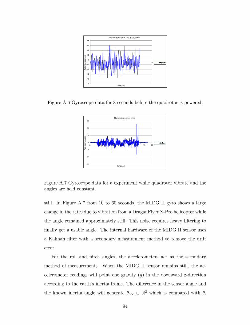
After mounting the MIDG II onto the DraganFlyer X-Pro seen in Figure
A.5, the actual MEMS gyro data itself is heavily noisy, as seen in Figure A.6
and A.7. Figure A.6 shows MIDG II gyro readings while the sensor remains
92
MIDG II
Figure A.5 The MIDG II mounted on the DraganFlyer X-Pro UAV
93
Gyro values over first 8 seconds
-1
-0.8
-0.6
-0.4
-0.2
0
0.2
0.4
0.6
0.8
0 2 4 6 8 10
Time(sec)R
ate
(deg
rees/s
ec)
?(pitch)
Figure A.6 Gyroscope data for 8 seconds before the quadrotor is powered.
Gyro values over time
-30
-20
-10
0
10
20
30
0 10 20 30 40 50 60 70 80
Time(sec)
Rate
(deg
rees/s
ec)
?(pitch)
Figure A.7 Gyroscope data for a experiment while quadrotor vibrate and theangles are held constant.
still. In Figure A.7 from 10 to 60 seconds, the MIDG II gyro shows a large
change in the rates due to vibration from a DraganFlyer X-Pro helicopter while
the angle remained approximately still. This noise requires heavy filtering to
finally get a usable angle. The internal hardware of the MIDG II sensor uses
a Kalman filter with a secondary measurement method to remove the drift
error.
For the roll and pitch angles, the accelerometers act as the secondary
method of measurements. When the MIDG II sensor remains still, the ac-
celerometer readings will point one gravity (g) in the downward z-direction
according to the earth’s inertia frame. The difference in the sensor angle and
the known inertia angle will generate θacc ∈ R2 which is compared with θi
94
(A.1) to generate the ωbias for the roll and pitch angles to correct for drift.
The yaw angle is independent from gravity and cannot use the gravity vec-
tor to correct for drift, so an additional sensor must be used for correcting the
yaw drift. The secondary yaw sensor used in the MIDG II is a 3-axis magne-
tometer. Throughout the earth surface a magnetic field can be measured. A
north seeking compass is a primitive tool that can detect this magnetic field.
A 3-axis magnetometer actually measures this magnetic force (in milligauss)
in the x-, y-, and z-directions. These three pieces of information are magni-
tudes and allow the sensor to know the 3-D magnetic vector. What is desired,
however, is the yaw orientation. By projecting the vector on the x-y plane,
the yaw angle can be calculated relative to the North Pole. This assumes the
magnetic field in the area is approximately the constant (north seeking). This
assumption holds true as long as the sensor is not near ferrites or magnetic
fields. Three scalars can be used to determine up to two orientations and one
magnitude, as shown in Figure A.8. A point, P , contains two angles (θ and φ)
and one magnitude (ρ). Since there are two angles in the 3-D magnetic vector
(OP ), it can potentially be used to measure a second orientation angle. How-
ever, this is not done since the accelerometers take care of pitch and roll. The
3-D magnetic vector cannot correct for a third orientation because the third
orientation rotates along the axis and cannot be measured. The accelerometers
follow the same reasoning and do correct for two orientations: pitch and roll.
With the accelerometers and magnetometers combined, three orientations are
measured. However, if the magnetic field and gravitational field line up, there
would be a singularity and one orientation cannot be measured. This does not
happen unless the magnetic field is no longer north seeking.
Both secondary measurement methods mentioned allow drift to be removed
and give a reference point to all orientations. For pitch and roll, zero degrees
is orthogonal to gravity. For yaw, zero degrees is north, assuming the mag-
netic field in the area is due to the earth’s magnetic field. The secondary
measurements are combined with the gyroscope data by Kalman filtering the
95
Figure A.8 Cartesian and Cylindrical coordinates
96
two together over time. This allows for the accelerometer vector to change a
little (by shaking the sensor around) without drastically changing the values
of pitch and roll, and allowing it to re-correct the values in seconds. In the
yaw case, a shift in the magnetic field causes the yaw heading to change in
only a few seconds. This is the cause for a great error in the yaw angle.
Magnetometer Problem
One of the applications for the MIDG II sensor is UAV application. Many
UAVs use gas power and will have no magnetic interference for the MIDG
II sensor. The DraganFlyer X-Pro is an electric helicopter with permanent
magnet motors and currents ranging from 30 to 70 amps (total current for
all four motors). The permanent magnets can be spaced 20 inches away from
the sensor, but the current is all over the DraganFlyer X-Pro and cannot be
avoided.
Figure A.9 shows a 3-D plot of magnetic field vectors shown as points in
x, y, and z from an experiment using the MIDG II on the DraganFlyer X-Pro.
The shift between the different ellipses shows the effects of interference in the
magnetic vectors. The magnetic field starts in ellipse a before the motors are
turned on. Ellipses b and c show an immediate shift in the direction of the
magnetic vector readings after turning on the helicopter. The magnetometer
readings vary throughout ellipses b and c depending on how much current
flows through the motors. The shift from ellipse a to b or c is across the x-
and y-axes, an error of up to 180◦. Such a large error is detrimental to the
operation of the sensor.
A magnetic source is not the only cause for disturbance in the earth’s mag-
netic field. The existence of a ferrous material alone can cause a shift in the
magnetic field, as shown in Figure A.10. Buildings, roads, and bridges com-
monly contain iron beams and rods for structural reinforcement. Rotomotion
uses a magnetometer for orientation data and cannot go near buildings for
this reason. This demonstrates one of the many possible errors observed when
97
a
b
c
Figure A.9 Magnetometer vector values
98
Figure A.10 Ferrous object disturbance in uniform magnetic field
using magnetometers.
Magnetometer Solution
The MIDG II sensor uses MEMS gyros for determining the orientations. If a
gyro is used by itself, there will always be a drift error due to a non-zero bias
and noise. The magnetometers are used to correct drift error over time by
monitoring the earth’s magnetic field for all time and continuously correcting
yaw ωbias (t).
The MIDG II sensor has three paths for the modes of operations: IMU,
VG, and INS. IMU path (Inertia Measurement Unit) is not used because it
only supplies raw unfiltered gyro and accelerometer information. INS (Inertia
Navigation System) path requires GPS and cannot be used inside of a building
where a majority of the experiments occur. The VG path (Vertical Gyro) uses
the gyros, accelerometers and magnetometers to generate yaw, pitch, and roll
values. The VG path has 5 sequential modes of operation: VG Initialize, VG
Fast, VG Med, VG Slow, and VG SE. Each mode is more accurate than the
last. VG SE mode can continue to INS path if GPS is engaged, or return to
VG Med mode if the gyro rates saturate (the sensor rotates too fast). To read
more about the different sensor modes, please see the MIDG II information
sheet “Operating Modes” [13].
Once in the VG SE mode, the MIDG II has a good estimation of the bias
in the system. The solution to the magnetometer problem is to correct for yaw
for only a limited period of time and not use the magnetometers in the VG
SE mode. If the magnetometers were simply not used in VG SE mode, then
99
(A.1) can be used with a constant value of ωbias for the yaw angle and any
drift error would only be due to variations in the yaw ωbias term. A modified
firmware is used to disable magnetometer readings in VG SE mode only.
It is important to have an accurate value of ωbias for yaw before entering
VG SE mode despite any magnetic interference. Even with the magnetometers
turned off in VG SE mode, if ωbias has a corrupted value there will be a large
drift over time due to the incorrect ωbias. To alleviate this problem, the sensor
remains motionless and the helicopter motors remain off until the sensor enters
VG SE mode. The only magnetic interferences that remain are fluctuations in
the magnetic fields due to ferrous materials, such as buildings. As long as the
magnetic field does not vary and does not line up with the gravitational field,
this solution works. There will still be a small drift error from the gyros, but
over a 15 minute time frame, it should be unnoticeable.
Upon implementing the new firmware, the magnetic interference due to
magnets and magnetic currents has no effect on the yaw reading at all. Micro-
botics Inc, maker of the MIDG II sensor stated that without the magnetometer
readings, the sensor can expect up to 5 degrees of error per minute. After a 10
minute experiment, there was an actual error of about 3 degrees. Even if there
was an error of 5 degrees a minute, it could be corrected with knowledge of the
sensor’s velocity. As the helicopter loses yaw, it would slowly move forward
in the wrong direction, and this can be detected and compensated for. It is
concluded that even a small 5 degrees per minute error would be acceptable,
given the 15 minute fly time of the DraganFlyer X-Pro.
GPS
The Differential GPS sensor is investigated to observer how it reacts under
normal conditions. In this experiment, the GPS sensor is positioned on top of
the Flour Daniel building and is held stationary while gathering data for 1 hour
and 45 minutes. All the GPS data from the MIDG II sensor is recorded during
this time. For this experiment, WAAS signals are not received. It has been
100
GPS Data (position)
-1200
-1000
-800
-600
-400
-200
0
200
400
600
0 1000 2000 3000 4000 5000 6000
Time(seconds)
Po
sit
ion
(cm
)
x(cm)
y(cm)
z(cm)
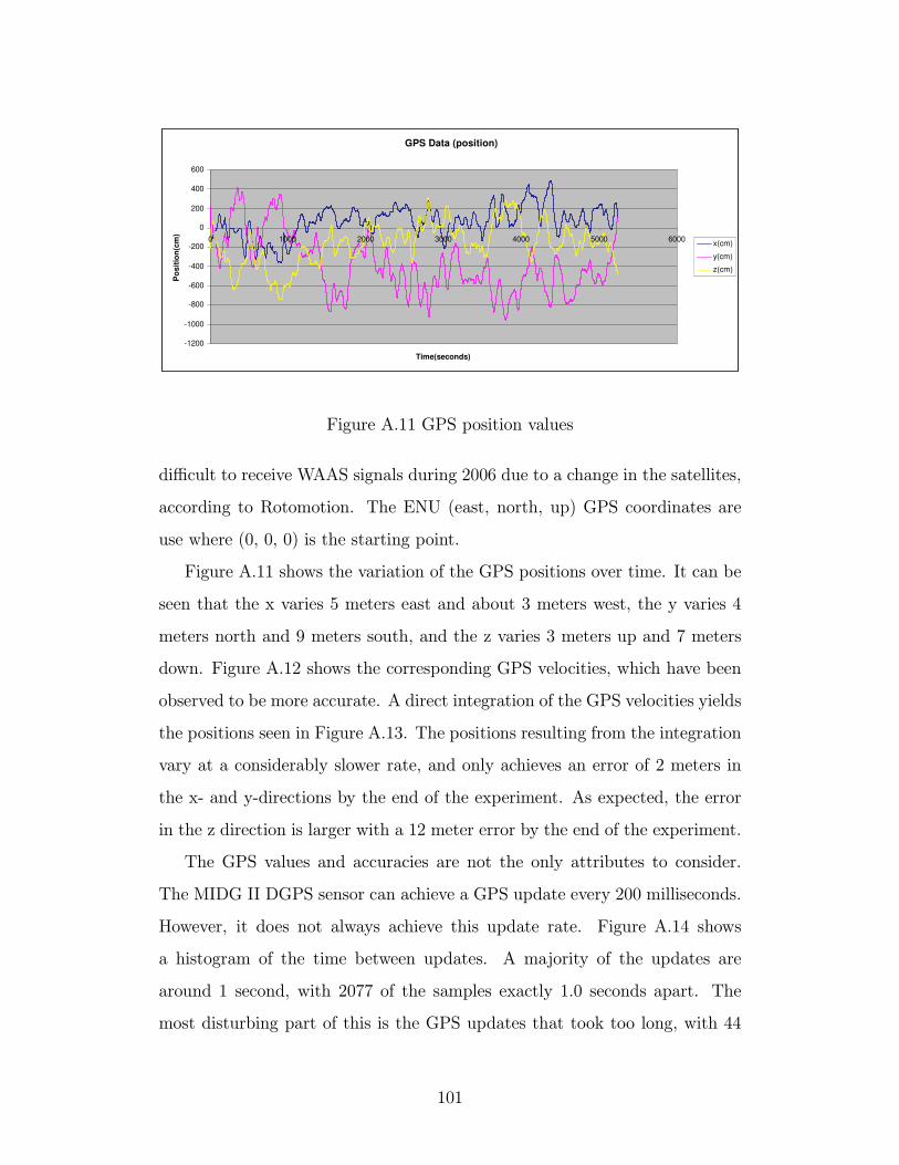
Figure A.11 GPS position values
difficult to receive WAAS signals during 2006 due to a change in the satellites,
according to Rotomotion. The ENU (east, north, up) GPS coordinates are
use where (0, 0, 0) is the starting point.
Figure A.11 shows the variation of the GPS positions over time. It can be
seen that the x varies 5 meters east and about 3 meters west, the y varies 4
meters north and 9 meters south, and the z varies 3 meters up and 7 meters
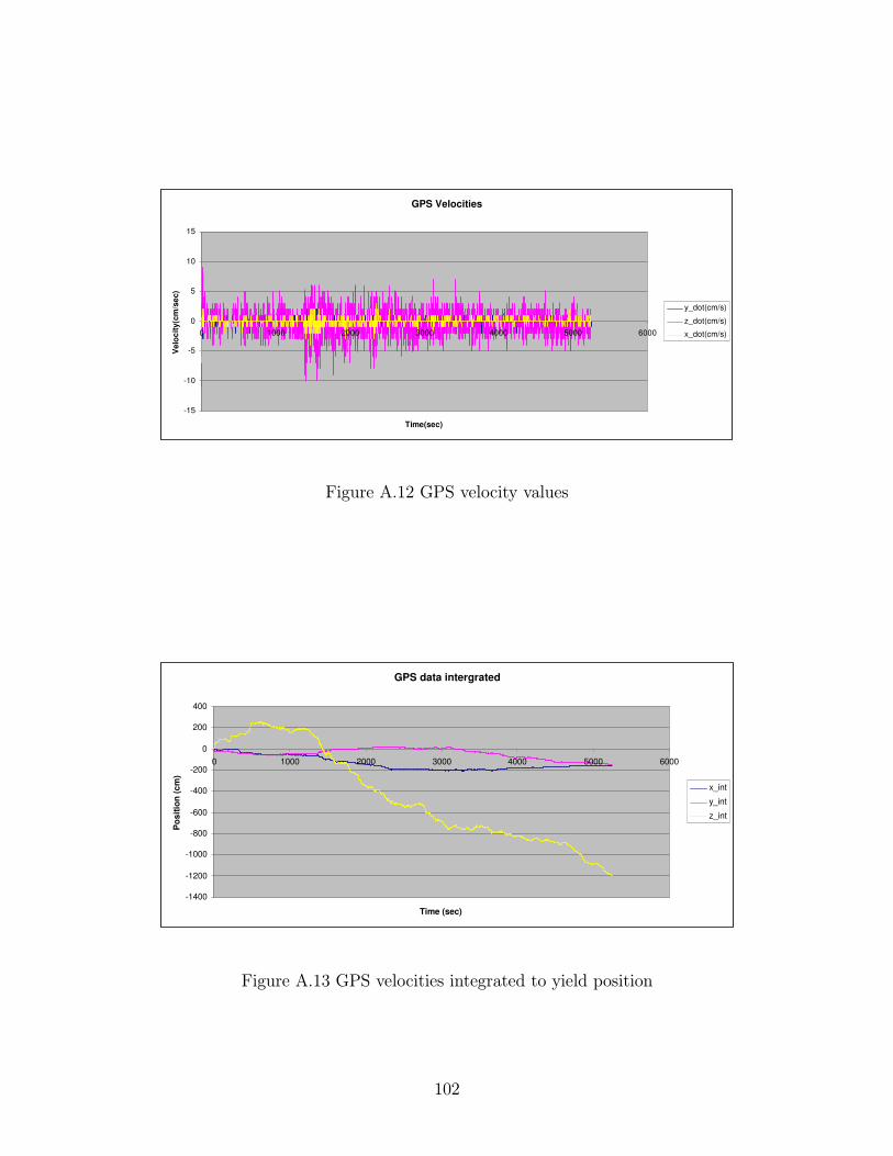
down. Figure A.12 shows the corresponding GPS velocities, which have been
observed to be more accurate. A direct integration of the GPS velocities yields
the positions seen in Figure A.13. The positions resulting from the integration
vary at a considerably slower rate, and only achieves an error of 2 meters in
the x- and y-directions by the end of the experiment. As expected, the error
in the z direction is larger with a 12 meter error by the end of the experiment.
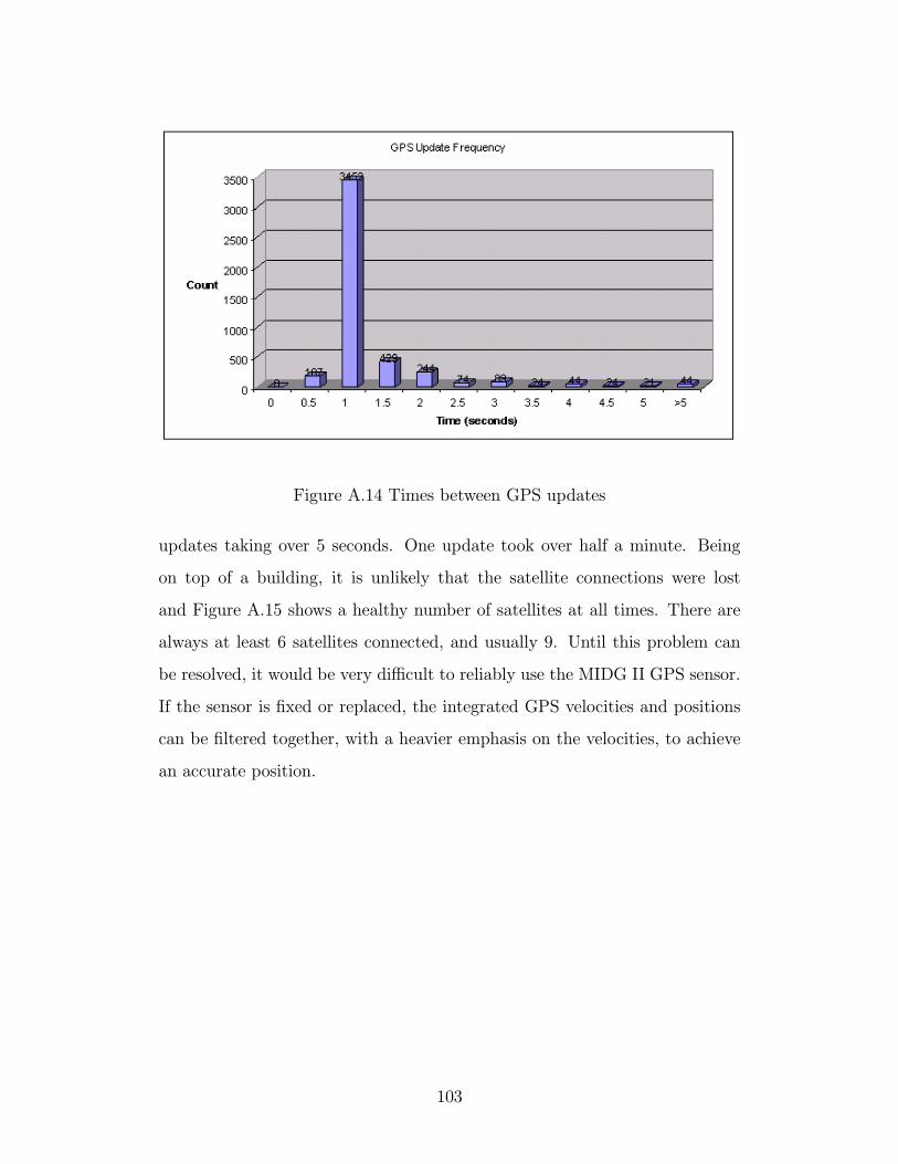
The GPS values and accuracies are not the only attributes to consider.
The MIDG II DGPS sensor can achieve a GPS update every 200 milliseconds.
However, it does not always achieve this update rate. Figure A.14 shows
a histogram of the time between updates. A majority of the updates are
around 1 second, with 2077 of the samples exactly 1.0 seconds apart. The
most disturbing part of this is the GPS updates that took too long, with 44
101
GPS Velocities
-15
-10
-5
0
5
10
15
0 1000 2000 3000 4000 5000 6000
Time(sec)
Ve
loc
ity(c
m/s
ec)
y_dot(cm/s)
z_dot(cm/s)
x_dot(cm/s)
Figure A.12 GPS velocity values
GPS data intergrated
-1400
-1200
-1000
-800
-600
-400
-200
0
200
400
0 1000 2000 3000 4000 5000 6000
Time (sec)
Po
sit
ion
(c
m)
x_int
y_int
z_int
Figure A.13 GPS velocities integrated to yield position
102
Figure A.14 Times between GPS updates
updates taking over 5 seconds. One update took over half a minute. Being
on top of a building, it is unlikely that the satellite connections were lost
and Figure A.15 shows a healthy number of satellites at all times. There are
always at least 6 satellites connected, and usually 9. Until this problem can
be resolved, it would be very difficult to reliably use the MIDG II GPS sensor.
If the sensor is fixed or replaced, the integrated GPS velocities and positions
can be filtered together, with a heavier emphasis on the velocities, to achieve
an accurate position.
103
365
842
1552
1751
122
0
200
400
600
800
1000
1200
1400
1600
1800
Count
6 7 8 9 10
Sattelites
Number of GPS Satellites
Figure A.15 Number of satellites receiving GPS signals from.
104
Appendix B
Signal Chasing for Theorem 1
According to Theorem 1 and its subsequent stability analysis from (3.62) to
(3.77), V (t) is bounded according to (3.77). Since the conditions in (3.71) and
(3.74) are guaranteed to be satisfied by some arbitrary variables that always
exist, it ensures that eω (t) and rv (t) are bounded. The desired trajectories,
vCICd (t) and ωCICd (t), are assumed to be bounded. The transformation matrices
R (Θ) and J−1F (Θ) are bounded under the assumption that θp = ±π2, based on
the definition of (3.10) and (3.11) which applies to all rotation matrices. Now
it can be said that ev (t) in (3.26) is bounded, resulting in vCIC (t) in (3.25) and
ωCIC (t) in (3.42) being bounded. Thus vFIF (t) ∈ L∞ by (3.28) which results
in xIIF (t) ∈ L∞ by (3.2). Since JC (t) ∈ L∞ by (3.19)/(3.23), all elements
of B (t) in (3.45) are bounded. ζ(∥∥vFIF (t)
∥∥) can be shown to be upper and
lower bounded by the inequality in (3.53). N1 (·) and g are assumed to be
bounded, yielding N11 (·) and G11 (·) ∈ L∞ by (3.37) and (3.38). Now U1 (t)
and U2 (t) can be shown to be bounded in (3.52) and the lower half of (3.48).
Owing to B (t) and U (t) ∈ L∞, U (t) is bounded by (3.46), yielding u1 (t),
ωFIF (t), and θC (t) are bounded. Thus ωFFC (t) is bounded by (3.43). Owing to
ωFFC (t) ∈ L∞, S(ωFFC (t)
)is also bounded by (3.6), resulting in RC
F (t) being
bounded by (3.30). Based on (3.10), JF (t) can be found to be
JF =
1 0 − sin (θ)0 cos (ψ) sin (ψ) cos (θ)0 − sin (ψ) cos (ψ) cos (θ)
, (B.1)
which is bounded. Since ωFIF (t) ∈ L∞, ΘFIF (t) is bounded by (3.8).
∥∥vCICd (t)∥∥
is assumed to be upper bounded by β1 (t) expressed in (3.67). Owing to
U (t) ∈ L∞, rv (t) is bounded by (3.41) and vFIF (t) ∈ L∞ by modeling equation
(3.3). Therefore, we can conclude that all signals are bounded in the velocity
control of fly-by-camera interface.
105
BIBLIOGRAPHY
[1] FlightGear, http://www.flightgear.org/.
[2] T. I. Fossen, Marine Control Systems : Guidance, Navigation, and Controlof Ships, Rigs, and Underwater Vehicles, Marine Cybernetics, 2002.
[3] T. Hamel, R. Mahony, R. Lozano, and J. Ostrowski, “Dynamic Modellingand Configuration Stabilization for an X-4 Flyer,” Proceedings of theIFAC World Congress, Barcelona, Spain, July 2002.
[4] V. Chitrakaran, D. Dawson, H. Kannan, and M. Feemster, “Vision-Based Tracking for Unmanned Aerial Vehicles.” Technical ReportCU/CRB/2/27/06/#1, College of Engineering and Science Controland Robotics, Clemson University, Feb. 2006.
[5] V. Chitrakaran, D. Dawson, J. Chen, and M. Feemster, “Vision AssistedAutonomous Landing of an Unmanned Aerial Vehicle,” Proceedingsof the IEEE Conf. on Decision and Control, Seville, Spain, pp. 1465-1470, December, 2005.
[6] P. Pounds, R. Mahony, J. Gresham, P. Corke, and J. Roberts, “TowardsDynamically-Favourable Quad-Rotor Aerial Robots,” Proc. of the2004 Australasian Conf. on Robotics and Automation, Canberra,Australia, Dec. 2004.
[7] G. Hoffmann, D. Rajnarayan, S. Waslander, D. Dostal, J. Jang, and C.Tomlin, “The Stanford Testbed of Autonomous Rotorcraft for MultiAgent Control (STARMAC)”, Proceedings of the 23rd Digital Avion-ics Systems Conference, Salt Lake City, Utah, pp. 12.E.4-12.E.10,November, 2004.
[8] J. Jang and C. Tomlin, “Longitudinal Stability Augmentation System De-sign for the DragonFly UAV using a Single GPS Receiver,” Proceed-ings of the AIAA Guidance, Navigation, and Control Conference,Austin, Texas, AIAA Paper Number 2003-5592, August 2003.
[9] A. Tayebi and S. McGilvray, “Attitude Stabilization of a VTOL QuadrotorAircraft”, IEEE Transactions on Control Systems Technology, pp.562-571, May 2006.
[10] T. Hamel and R. Mahony, “Attitude estimation on SO(3) based on directinertial measurements”, Proc. of the 2006 IEEE Int. Conf. on Ro-botics and Automation, Orlando, Florida, pp. 2170-2175, May 2006.
[11] P. McKerrow, “Modelling the Draganflyer Four-Rotor Helicopter”, Proc.of the 2004 IEEE Int. Conf. on Robotics and Automation, pp. 3596-3601, New Orleans, April 2004.
[12] S. Bouabdallah, P. Murrieri, and R. Siegwart, “Design and control of an in-door micro quadrotor”, Proc. of the 2004 IEEE Int. Conf. on Robot-ics and Automation, New Orleans, Louisiana, pp. 4393-4398, April2004.
[13] MIDG II INS/GPS Sensor, http://microboticsinc.com/ins gps.php.