Elementi di Meccanica Computazionale Corso di Laurea in Ingegneria Civile Pavia, 2014 Linear beams: extension to dynamics and finite element formulation Ferdinando Auricchio 12 1 DICAR – Dipartimento di Ingegneria Civile e Architettura, Universit` a di Pavia, Italy 2 IMATI – Istituto di Matematica Applicata e Tecnologie Informatiche, CNR, Italy March 13, 2014 F.Auricchio (UNIPV) Linear beam March 13, 2014 1 / 44
Transcript
Elementi di Meccanica ComputazionaleCorso di Laurea in Ingegneria Civile
Pavia, 2014
Linear beams: extension to dynamics and finite element
formulation
Ferdinando Auricchio 1 2
1DICAR – Dipartimento di Ingegneria Civile e Architettura, Universita di Pavia, Italy2IMATI – Istituto di Matematica Applicata e Tecnologie Informatiche, CNR, Italy
March 13, 2014
F.Auricchio (UNIPV) Linear beam March 13, 2014 1 / 44
Some references I
A. Chopra, “Dynamics of Structures: Theory and Applications to EarthquakeEngineering (2nd Edition) ”, Prentice Hall, 2000
F.Auricchio (UNIPV) Linear beam March 13, 2014 2 / 44
Beam: extension to dynamics I
GOAL: extend beam formulation to include dynamics
1 Weak formulation of the problem
Differential form → Integro-differential form
2 Introduction of approximation fields
Integro-differential form → Algebraic-differential form
3 Introduction of time-marching scheme
Algebraic-differential form → Algebraic form
4 Solution of algebraic problem
F.Auricchio (UNIPV) Linear beam March 13, 2014 3 / 44
Beam: extension to dynamics at the continuous level I
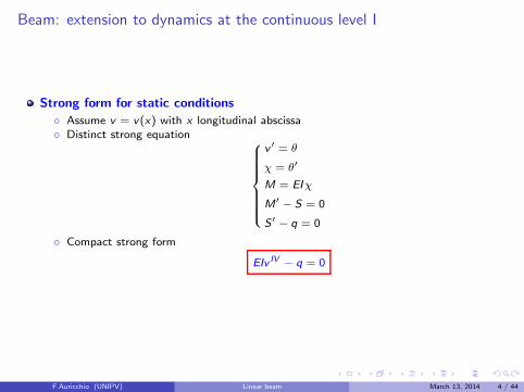
Strong form for static conditions
◦ Assume v = v(x) with x longitudinal abscissa◦ Distinct strong equation
v ′ = θ
χ = θ′
M = EIχ
M′ − S = 0
S ′ − q = 0
◦ Compact strong form
EIv IV − q = 0
F.Auricchio (UNIPV) Linear beam March 13, 2014 4 / 44
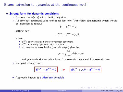
Beam: extension to dynamics at the continuous level II
Strong form for dynamic conditions
◦ Assume v = v(x , t) with t indicating time◦ All previous equations valid except for last one (transverse equilibrium) which should
be modified as follow:S ′ − qdyn = 0
setting now
qdyn = qstat − ρv v
where⋆ qdyn : equivalent load under dynamical conditions⋆ qstat : externally applied load (static load)⋆ ρv : transverse mass density (per unit length) given by
ρv =
∫
h/2
−h/2
ρbdy = ρA
with ρ mass density per unit volume, b cross-section depth and A cross-section area
◦ Compact strong form
EIv IV − qdyn = 0 or EIv IV + ρv v − qstat = 0
◮ Approach known as d’Alembert principle
F.Auricchio (UNIPV) Linear beam March 13, 2014 5 / 44
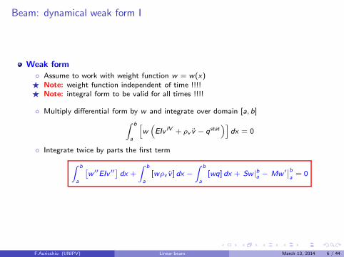
Beam: dynamical weak form I
Weak form
◦ Assume to work with weight function w = w(x)⋆ Note: weight function independent of time !!!!⋆ Note: integral form to be valid for all times !!!!
◦ Multiply differential form by w and integrate over domain [a,b]
∫ b
a
[
w(
EIv IV + ρv v − qstat)]
dx = 0
◦ Integrate twice by parts the first term
∫ b
a
[
w ′′EIv ′′]
dx +
∫ b
a
[wρv v ] dx −
∫ b
a
[wq] dx + Sw |ba − Mw ′∣
∣
b
a= 0
F.Auricchio (UNIPV) Linear beam March 13, 2014 6 / 44
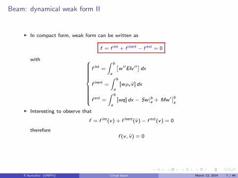
Beam: dynamical weak form II
◮ In compact form, weak form can be written as
f = f int + f inert − f ext = 0
with
f int =
∫ b
a
[
w ′′EIv ′′]
dx
f inert =
∫ b
a
[wρv v ] dx
f ext =
∫ b
a
[wq] dx − Sw |ba + Mw ′∣
∣
b
a
◮ Interesting to observe that
f = f int(v) + f inert(v)− f ext(v) = 0
thereforef (v , v) = 0
F.Auricchio (UNIPV) Linear beam March 13, 2014 7 / 44
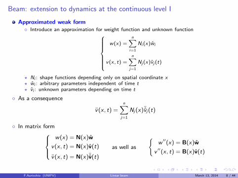
Beam: extension to dynamics at the continuous level I
Approximated weak form
◦ Introduce an approximation for weight function and unknown function
w(x) =n
∑
i=1
Ni (x)wi
v(x , t) =n
∑
j=1
Nj(x)vj (t)
⋆ Ni : shape functions depending only on spatial coordinate x⋆ wi : arbitrary parameters independent of time t⋆ vi : unknown parameters depending on time t
◦ As a consequence
v(x , t) =
n∑
j=1
Nj (x)¨vj (t)
◦ In matrix form
w(x) = N(x)w
v(x , t) = N(x)v(t)
v(x , t) = N(x)¨v(t)
as well as
{
w′′(x) = B(x)w
v′′(x , t) = B(x)v(t)
F.Auricchio (UNIPV) Linear beam March 13, 2014 8 / 44
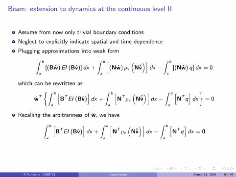
Beam: extension to dynamics at the continuous level II
Assume from now only trivial boundary conditions
Neglect to explicitly indicate spatial and time dependence
Plugging approximations into weak form
∫ b
a
[(Bw)EI (Bv)] dx +
∫ b
a
[
(Nw) ρv(
N¨v)]
dx −
∫ b
a
[(Nw) q] dx = 0
which can be rewritten as
wT
{∫ b
a
[
BTEI (Bv)
]
dx +
∫ b
a
[
NTρv
(
N¨v)]
dx −
∫ b
a
[
NTq]
dx
}
= 0
Recalling the arbitrariness of w, we have
∫ b
a
[
BTEI (Bv)
]
dx +
∫ b
a
[
NTρv
(
N¨v)]
dx −
∫ b
a
[
NTq]
dx = 0
F.Auricchio (UNIPV) Linear beam March 13, 2014 9 / 44
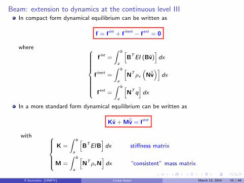
Beam: extension to dynamics at the continuous level IIIIn compact form dynamical equilibrium can be written as
f = fint + f
inert− f
ext = 0
where
fint =
∫ b
a
[
BTEI (Bv)
]
dx
finert =
∫ b
a
[
NTρv
(
N¨v)]
dx
fext =
∫ b
a
[
NTq]
dx
In a more standard form dynamical equilibrium can be written as
Kv +M¨v = fext
with
K =
∫ b
a
[
BTEIB
]
dx stiffness matrix
M =
∫ b
a
[
NTρvN
]
dx “consistent” mass matrix
F.Auricchio (UNIPV) Linear beam March 13, 2014 10 / 44
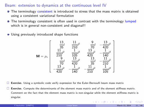
Beam: extension to dynamics at the continuous level IV
The terminology consistent is introduced to stress that the mass matrix is obtainedusing a consistent variational formulation
The terminology consistent is often used in contrast with the terminology lumpedwhich is in general non-consistent and diagonal!!
Using previously introduced shape functions
M = ρv
13
35l
11
210l2
9
70l −
13
420l2
11
210l2
1
105l3
13
420l2 −
1
140l3
9
70l
13
420l2
13
35l −
11
210l2
−13
420l2 −
1
140l3 −
11
210l2
1
105l3
� Exercise. Using a symbolic code verify expression for the Euler-Bernoulli beam mass matrix
� Exercise. Compute the determinants of the element mass matrix and of the element stiffness matrix.
Comment on the fact that the element mass matrix is non-singular while the element stiffness matrix is
singular.
F.Auricchio (UNIPV) Linear beam March 13, 2014 11 / 44
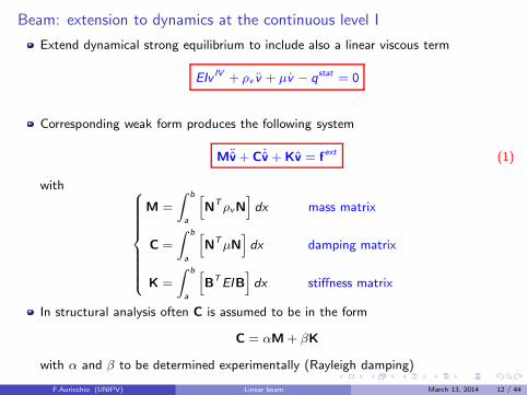
Beam: extension to dynamics at the continuous level I
Extend dynamical strong equilibrium to include also a linear viscous term
EIvIV + ρv v + µv − q
stat = 0
Corresponding weak form produces the following system
M¨v+ C ˙v+ Kv = fext (1)
with
M =
∫ b
a
[
NTρvN
]
dx mass matrix
C =
∫ b
a
[
NTµN
]
dx damping matrix
K =
∫ b
a
[
BTEIB
]
dx stiffness matrix
In structural analysis often C is assumed to be in the form
C = αM+ βK
with α and β to be determined experimentally (Rayleigh damping)
F.Auricchio (UNIPV) Linear beam March 13, 2014 12 / 44
Dynamic problem: problem classification I
As a result of semi-discretization in space, time-dependent problem is reduced to aset of ordinary differential equations
In the following discuss three different possible situations:
◦ Determination of free-response (i.e. fext = 0)
◦ Determination of steady-state periodic response (i.e. fext periodic in time)◦ Determination of transient response (i.e. fext arbitrary in time)
F.Auricchio (UNIPV) Linear beam March 13, 2014 13 / 44
Dynamic problem: free-response / eigenvalue problem I
From now on consider always discrete problems (i.e. simplify notation)
If no damping or forcing terms exist, dynamical problem 1 reduces as
Mu+ Ku = 0 (2)
A general solution can be written in the form
u = u exp(iωt)
with the corresponding real part representing an harmonic response since
exp(iωt) = cos(ωt) + i sin(ωt)
Back-substitution into equation 2 returns(
−ω2M+ K
)
u = 0 (3)
i.e. a general linear eigenvalue or characteristic value problem and for non-zerosolutions the determinant of the above coefficient matrix must be zero
det[
−ω2M+ K
]
= 0 (4)
F.Auricchio (UNIPV) Linear beam March 13, 2014 14 / 44
Dynamic problem: free-response / eigenvalue problem II
Provided that M and K are n × n symmetric-definite matrices, condition 4 gives npositive roots or eigenvalues ωi with i = 1..n
For each eigenvalue, using equation 3, possible to compute system eigenvectors ornormal modes ui , in general requiring a proper normalization, i.e. s.t.
uTi Mui = 1 for i = 1..n
At this stage also possible to introduce classical modal orthogonality condition
uTi Muj = u
Tj Mui = 0 for i 6= j
as well as to prove the result
uTi Kui = ω
2i
F.Auricchio (UNIPV) Linear beam March 13, 2014 15 / 44
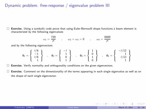
Dynamic problem: free-response / eigenvalue problem III
� Exercise. Using a symbolic code prove that using Euler-Bernoulli shape functions a beam element ischaracterized by the following eigenvalues
ω1 =720
l4, ω2 = ω3 = 0 , ω4 =
8400
l4
and by the following eigenvectors
u1 =
l/6−1l/61
, u2 =
−l
101
, u3 =
1010
, u4 =
−l/121
l/121
� Exercise. Verify normality and orthogonality conditions on the given eigenvectors.
� Exercise. Comment on the dimensionality of the terms appearing in each single eigenvalue as well as on
the shape of each single eigenvector.
F.Auricchio (UNIPV) Linear beam March 13, 2014 16 / 44
Dynamic problem: free-response / eigenvalue problem IV
To preserve methods based on the invertibility of stiffness matrix, possible to use anartifice
Modify problem[
−ω2M+ K
]
u = 0
into[
−(
ω2 + α
)
M+ (K+ αM)]
u = 0
where α is an arbitrary constant of the same order of the typical ω2 sought
The new matrix K+ αM is no more singular
F.Auricchio (UNIPV) Linear beam March 13, 2014 17 / 44
Dynamic problem: damped free-response / eigenvalue problem I
If damping exists but no no forcing terms exist , dynamical problem 1 reduces as
Mu+ Cu+ Ku = 0 (5)
A general solution can again be written in the form
u = u exp(αt)
Back-substitution into equation 5 returns
(
α2M+ αC+ K
)
u = 0 (6)
with α and u possibly complex quantities, with a real part representing a decayingvibration
Equation 6 corresponds again to an eigenvalue problem, which is more complex thanthe one previously considered
F.Auricchio (UNIPV) Linear beam March 13, 2014 18 / 44
Dynamic problem: damped free-response / eigenvalue problem II
Usually the problem is solved by splitting it into two first-order problems, defining
u = v
s.t. we get
[
M 0
0 −M
]{
v
u
}
+
[
C K
M 0
]{
v
u
}
=
{
0
0
}
Setting now
u = u exp(αt) , v = v exp(αt)
and substituting gives the general linear eigenvalue
(
α
[
M 0
0 −M
]
+
[
C K
M 0
]){
v
u
}
=
{
0
0
}
(7)
F.Auricchio (UNIPV) Linear beam March 13, 2014 19 / 44
Dynamic problem: forced periodic response I
If in equation 1 the forcing term is periodical, i.e.
f = f exp(αt)
with α = α1 + iα2, then general solution can be again written as
u = u exp(αt)
which plugged into 1 gives
(
α2M+ αC+K
)
u = f
Obtained problem is no more an eigenvalue problem and it can simply solved as
u = K−1
f
where
K = α2M + αC+ K
F.Auricchio (UNIPV) Linear beam March 13, 2014 20 / 44
Dynamic problem: transient response procedures I
To treat the response of a linear dynamical system to a general force we can adopttwo approaches:
◦ frequency response procedures◦ numerical time-integration
⋆ Start considering frequency response procedures
In general a completely arbitrary forcing function can be represented approximatelyby a Fourier series or in the limit, exactly, as a Fourier integral
Accordingly, response to a completely arbitrary forcing function can be obtainedproperly combining the response to a series of periodic forcing functions
The frequency response technique is readily adapted to problems where the matrix C
is of an arbitrary form
F.Auricchio (UNIPV) Linear beam March 13, 2014 21 / 44
Dynamic problem: modal decomposition analysis I
For free response the general solution is of the form
u =n
∑
i
ui exp(αi t)
where αi are the complex eigenvalues and ui are the complex eigenvectors.
For forced response and linear problem, the solution can be again expressed as alinear combination of the modes
u =
n∑
i
uiyi (t) (8)
with yi scalar modal partecipation factors, assumed to be function of time
Position 8 presents no restriction as all the modes are linearly indipendent
F.Auricchio (UNIPV) Linear beam March 13, 2014 22 / 44
Dynamic problem: modal decomposition analysis II
Using position 8 in dynamical equation and premultiplying by the complex conjugateeigenvectors uT
i , the result is simply a set of scalar, indipendent equations
mi y + ci y + kiyi = fi (9)
where
mi = uTi Mui , ci = u
Ti Cui , ki = u
Ti Kui , fi = u
Ti f
since we have
uTi Muj = u
Ti Cuj = u
Ti Kuj = 0 when i 6= j
Each scalar equation 9 can be solved indipendently by elementary procedures
Total motion is obtained by superposition using 8
F.Auricchio (UNIPV) Linear beam March 13, 2014 23 / 44
Dynamic problem: modal decomposition analysis III
Most classical approach is to work with real eigenvalues obtained as solution of
[
−ω2M+ K
]
u = 0
With this position decoupled equations only in the case
uiCuj = 0 if i 6= j
which is a non-trivial condition since eigenvectors in general guarantee orthogonalitywrt M and K and not necessarily wrt C
If using damping matrix in the form of Rayleigh damping, then trivial.
F.Auricchio (UNIPV) Linear beam March 13, 2014 24 / 44
Exercises I
� Exercise. Modify the frame Matlab code to compute also mass matrix, structural eigenvalues andeigenmodes.
� Exercise. For some simple beam problems (i.e. simply supported or cantilever beams), computeeigenvalue and eigenvector solutions in close form and compare with numerical solutions obtained for anincreasing number of elements. Plot convergence diagrams in a log-log-scale.
� Exercise. Choose a structure and compute free response comparing it with a standard commercialsoftware.
� Exercise. Develop mass matrix for a Timoshenko beam model
F.Auricchio (UNIPV) Linear beam March 13, 2014 25 / 44
MDOF numerical solution I
Analytical solutions previously described provide insights into the behaviour patternsof linear systems
◦ Not computationally economical for the solution of transient problems◦ Cannot be extended to nonlinear cases
We now investigate discretization methods directly applicable to time-domain
Since time domain is infinite, refer to a finite time increment ∆t between tn andtn+1 = tn +∆t, obtaining the so-called recurrence relations
F.Auricchio (UNIPV) Linear beam March 13, 2014 26 / 44
MDOF numerical solution II
GOAL: solve equation of motion for a general load condition and possibly forgeneral internal force response
Time interval of interest: [0,T ]
Discretize time interval in N time sub-intervals of size ∆t, such that
t0 = 0, t1 = ∆t, t2 = 2∆t, .... tN = N∆t = T
or assume variable time sub-intervals
Resort to time-marching numerical scheme to compute motion in time, i.e.assuming to know solutions up to tn, compute solution at tn+1
Look for numerical solutions with a bounded error wrt exact solution, i.e.
un+1 ≈ u(tn+1) such that un+1 = u(tn+1) + O(∆tk)
then time integration method is k-order accurate
Second order accurate methods are desirable !!!!
F.Auricchio (UNIPV) Linear beam March 13, 2014 27 / 44
MDOF numerical solution: central difference method I
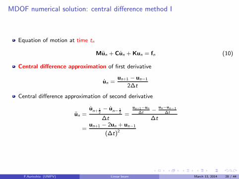
Equation of motion at time tn
Mun + Cun + Kun = fn (10)
Central difference approximation of first derivative
un =un+1 − un−1
2∆t
Central difference approximation of second derivative
un =un+ 1
2− un− 1
2
∆t=
un+1−un∆t
−un−un−1
∆t
∆t
=un+1 − 2un + un−1
(∆t)2
F.Auricchio (UNIPV) Linear beam March 13, 2014 28 / 44
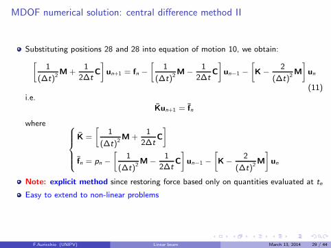
MDOF numerical solution: central difference method II
Substituting positions 28 and 28 into equation of motion 10, we obtain:
[
1
(∆t)2M+
1
2∆tC
]
un+1 = fn −
[
1
(∆t)2M−
1
2∆tC
]
un−1 −
[
K −2
(∆t)2M
]
un
(11)i.e.
Kun+1 = fn
where
K =
[
1
(∆t)2M+
1
2∆tC
]
fn = pn −
[
1
(∆t)2M−
1
2∆tC
]
un−1 −
[
K−2
(∆t)2M
]
un
Note: explicit method since restoring force based only on quantities evaluated at tn
Easy to extend to non-linear problems
F.Auricchio (UNIPV) Linear beam March 13, 2014 29 / 44
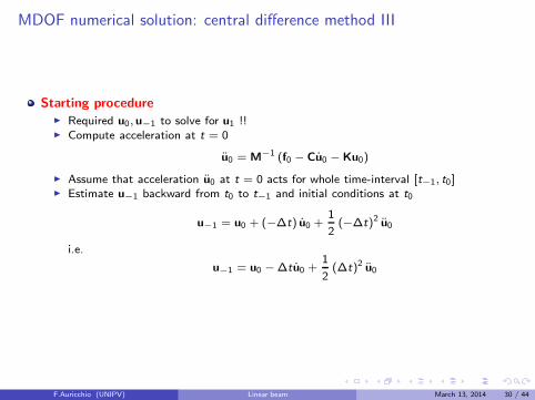
MDOF numerical solution: central difference method III
Starting procedure◮ Required u0, u−1 to solve for u1 !!◮ Compute acceleration at t = 0
u0 = M−1 (f0 − Cu0 − Ku0)
◮ Assume that acceleration u0 at t = 0 acts for whole time-interval [t−1, t0]◮ Estimate u−1 backward from t0 to t−1 and initial conditions at t0
u−1 = u0 + (−∆t) u0 +1
2(−∆t)2 u0
i.e.
u−1 = u0 −∆tu0 +1
2(∆t)2 u0
F.Auricchio (UNIPV) Linear beam March 13, 2014 30 / 44
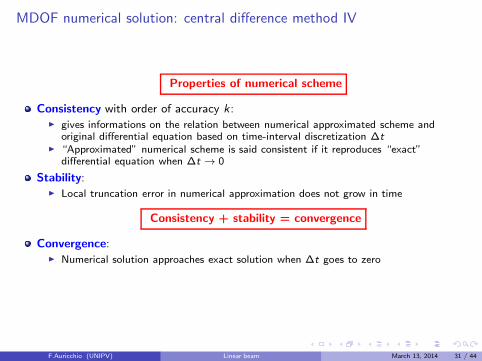
MDOF numerical solution: central difference method IV
Properties of numerical scheme
Consistency with order of accuracy k :◮ gives informations on the relation between numerical approximated scheme and
original differential equation based on time-interval discretization ∆t◮ “Approximated” numerical scheme is said consistent if it reproduces “exact”
differential equation when ∆t → 0
Stability:◮ Local truncation error in numerical approximation does not grow in time
Consistency + stability = convergence
Convergence:◮ Numerical solution approaches exact solution when ∆t goes to zero
F.Auricchio (UNIPV) Linear beam March 13, 2014 31 / 44
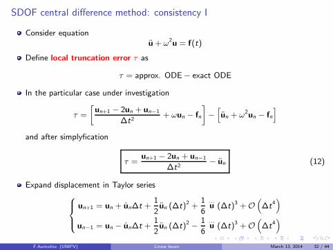
SDOF central difference method: consistency I
Consider equationu+ ω
2u = f(t)
Define local truncation error τ as
τ = approx. ODE− exact ODE
In the particular case under investigation
τ =
[
un+1 − 2un + un−1
∆t2+ ωun − fn
]
−[
un + ω2un − fn
]
and after simplyfication
τ =un+1 − 2un + un−1
∆t2− un (12)
Expand displacement in Taylor series
un+1 = un + un∆t +1
2un (∆t)2 +
1
6
...
u (∆t)3 +O(
∆t4)
un−1 = un − un∆t +1
2un (∆t)2 −
1
6
...
u (∆t)3 +O(
∆t4)
F.Auricchio (UNIPV) Linear beam March 13, 2014 32 / 44
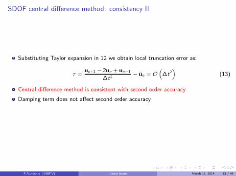
SDOF central difference method: consistency II
Substituting Taylor expansion in 12 we obtain local truncation error as:
τ =un+1 − 2un + un−1
∆t2− un = O
(
∆t2)
(13)
Central difference method is consistent with second order accuracy
Damping term does not affect second order accuracy
F.Auricchio (UNIPV) Linear beam March 13, 2014 33 / 44
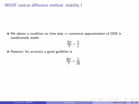
MDOF central difference method: stability I
We obtain a condition on time step ⇒ numerical approximation of ODE isconditionally stable
∆t
T<
1
π
However, for accuracy a good guideline is
∆t
T<
1
10
F.Auricchio (UNIPV) Linear beam March 13, 2014 34 / 44
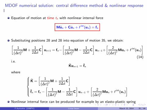
MDOF numerical solution: central difference method & nonlinear responseI
Equation of motion at time tn with nonlinear internal force
Mun + Cun + fint(un) = fn
Substituting positions 28 and 28 into equation of motion 35, we obtain:[
1
(∆t)2M+
1
2∆tC
]
un+1 = fn−
[
1
(∆t)2M−
1
2∆tC
]
un−1+
[
2
(∆t)2Mun + f
int(un)
]
(14)i.e.
Kun+1 = fn
where
K =
[
1
(∆t)2M+
1
2∆tC
]
fn = fn −
[
1
(∆t)2M−
1
2∆tC
]
un−1 +
[
2
(∆t)2Mun + f
int(un)
]
Nonlinear internal force can be produced for example by an elasto-plastic spring
F.Auricchio (UNIPV) Linear beam March 13, 2014 35 / 44
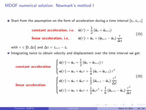
MDOF numerical solution: Newmark’s method I
Start from the assumption on the form of acceleration during a time interval [tn, tn+1]
constant acceleration, i.e. u(τ ) =1
2(un + un+1)
linear acceleration, i.e. u(τ ) = un + (un+1 − un)τ
∆t
(15)
with τ ∈ [0,∆t] and ∆t = tn+1 − tn
Integrating twice to obtain velocity and displacement over the time interval we get:
constant acceleration
u(τ ) = un +1
2(un + un+1) τ
u(τ ) = un + unτ +1
4(un + un+1) τ
2
linear acceleration
u(τ ) = un + unτ +1
2(un+1 − un)
τ 2
∆t
u(τ ) = un + unτ +1
2unτ
2 +1
6(un+1 − un)
τ 3
∆t
(16)
F.Auricchio (UNIPV) Linear beam March 13, 2014 36 / 44
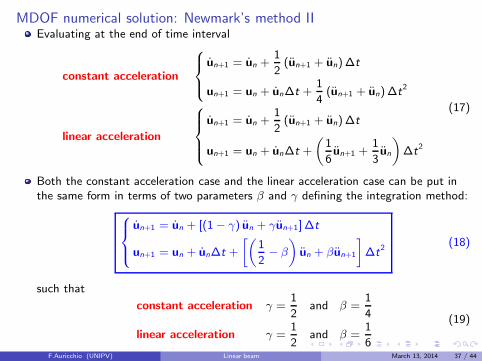
MDOF numerical solution: Newmark’s method IIEvaluating at the end of time interval
constant acceleration
un+1 = un +1
2(un+1 + un)∆t
un+1 = un + un∆t +1
4(un+1 + un)∆t
2
linear acceleration
un+1 = un +1
2(un+1 + un)∆t
un+1 = un + un∆t +
(
1
6un+1 +
1
3un
)
∆t2
(17)
Both the constant acceleration case and the linear acceleration case can be put inthe same form in terms of two parameters β and γ defining the integration method:
un+1 = un + [(1− γ) un + γun+1]∆t
un+1 = un + un∆t +
[(
1
2− β
)
un + βun+1
]
∆t2
(18)
such that
constant acceleration γ =1
2and β =
1
4
linear acceleration γ =1
2and β =
1
6
(19)
F.Auricchio (UNIPV) Linear beam March 13, 2014 37 / 44
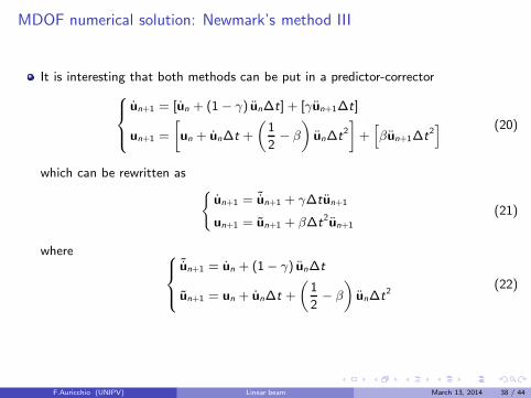
MDOF numerical solution: Newmark’s method III
It is interesting that both methods can be put in a predictor-corrector
un+1 = [un + (1− γ) un∆t] + [γun+1∆t]
un+1 =
[
un + un∆t +
(
1
2− β
)
un∆t2
]
+[
βun+1∆t2] (20)
which can be rewritten as{
un+1 = ˜un+1 + γ∆tun+1
un+1 = un+1 + β∆t2un+1
(21)
where
˜un+1 = un + (1− γ) un∆t
un+1 = un + un∆t +
(
1
2− β
)
un∆t2
(22)
F.Auricchio (UNIPV) Linear beam March 13, 2014 38 / 44
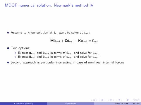
MDOF numerical solution: Newmark’s method IV
Assume to know solution at tn, want to solve at tn+1
Mun+1 + Cun+1 + Kun+1 = fn+1
Two options:
◦ Express un+1 and un+1 in terms of un+1 and solve for un+1
◦ Express un+1 and un+1 in terms of un+1 and solve for un+1
Second approach is particular interesting in case of nonlinear internal forces
F.Auricchio (UNIPV) Linear beam March 13, 2014 39 / 44
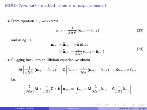
MDOF Newmark’s method in terms of displacements I
From equation 212 we express
un+1 =1
β∆t2(un+1 − un+1) (23)
and using 211un+1 = ˜un+1 + γ∆tun+1
= ˜un+1 +γ
β∆t(un+1 − un+1)
(24)
Plugging back into equilibrium equation we obtain
M
[
1
β∆t2(un+1 − un+1)
]
+ C
[
˜un+1 +γ
β∆t(un+1 − un+1)
]
+Kun+1 = fn+1
i.e.[
1
β∆t2M+
γ
β∆tC+ K
]
un+1 =
[
fn+1 +M1
β∆t2un+1 + C
γ
β∆tun+1
]
F.Auricchio (UNIPV) Linear beam March 13, 2014 40 / 44
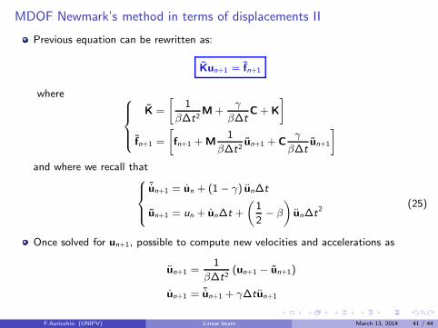
MDOF Newmark’s method in terms of displacements II
Previous equation can be rewritten as:
Kun+1 = fn+1
where
K =
[
1
β∆t2M+
γ
β∆tC+ K
]
fn+1 =
[
fn+1 +M1
β∆t2un+1 + C
γ
β∆tun+1
]
and where we recall that
˜un+1 = un + (1− γ) un∆t
un+1 = un + un∆t +
(
1
2− β
)
un∆t2
(25)
Once solved for un+1, possible to compute new velocities and accelerations as
un+1 =1
β∆t2(un+1 − un+1)
un+1 = ˜un+1 + γ∆tun+1
F.Auricchio (UNIPV) Linear beam March 13, 2014 41 / 44
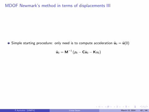
MDOF Newmark’s method in terms of displacements III
Simple starting procedure: only need is to compute acceleration u0 = u(0)
u0 = M−1 (p0 − Cu0 − Ku0)
F.Auricchio (UNIPV) Linear beam March 13, 2014 42 / 44
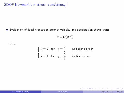
SDOF Newmark’s method: consistency I
Evaluation of local truncation error of velocity and acceleration shows that:
τ = O(∆tk)
with:
k = 2 for γ =1
2i.e second order
k = 1 for γ 6=1
2i.e first order
F.Auricchio (UNIPV) Linear beam March 13, 2014 43 / 44
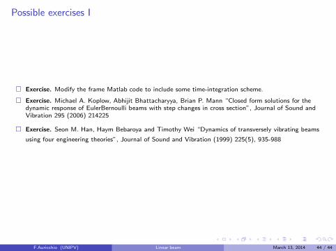
Possible exercises I
� Exercise. Modify the frame Matlab code to include some time-integration scheme.
� Exercise. Michael A. Koplow, Abhijit Bhattacharyya, Brian P. Mann “Closed form solutions for thedynamic response of EulerBernoulli beams with step changes in cross section”, Journal of Sound andVibration 295 (2006) 214225
� Exercise. Seon M. Han, Haym Bebaroya and Timothy Wei “Dynamics of transversely vibrating beams
using four engineering theories”, Journal of Sound and Vibration (1999) 225(5), 935-988
F.Auricchio (UNIPV) Linear beam March 13, 2014 44 / 44