Journal of Sound and < ibration (1999) 225(5), 935 } 988 Article No. jsvi.1999.2257, available online at http://www.idealibrary.com on DYNAMICS OF TRANSVERSELY VIBRATING BEAMS USING FOUR ENGINEERING THEORIES SEON M. HAN,HAYM BENAROYA AND TIMOTHY WEI Mechanical and Aerospace Engineering, Rutgers, the State ;niversity of New Jersey, Piscataway, NJ 08854, ;.S.A. (Received 18 September 1998, and in ,nal form 22 March 1999) In this paper, the full development and analysis of four models for the transversely vibrating uniform beam are presented. The four theories are the Euler}Bernoulli, Rayleigh, shear and Timoshenko. First, a brief history of the development of each beam model is presented. Second, the equation of motion for each model, and the expressions for boundary conditions are obtained using Hamilton's variational principle. Third, the frequency equations are obtained for four sets of end conditions: free} free, clamped}clamped, hinged}hinged and clamped}free. The roots of the frequency equations are presented in terms of normalized wave numbers. The normalized wave numbers for the other six sets of end conditions are obtained using the analysis of symmetric and antisymmetric modes. Fourth, the orthogonality conditions of the eigenfunctions or mode shape and the procedure to obtain the forced response using the method of eigenfunction expansion is presented. Finally, a numerical example is shown for a non-slender beam to signify the di!erences among the four beam models. ( 1999 Academic Press 1. INTRODUCTION The beam theories that we consider here were all introduced by 1921. That is, the problem of the transversely vibrating beam was formulated in terms of the partial di!erential equation of motion, an external forcing function, boundary conditions and initial conditions. Many e!orts had been devoted to obtaining and to understanding the solution of this non-homogeneous initial-boundary-value problem. However, work on this subject was done in a patchwork fashion by showing parts of the solution at a time, and there is no paper that presents the complete solution from the formulation of the governing di!erential equation to its solution for all four models. The most complete study was done by Traill-Nash and Collar [1], but they only derived the frequency equations for various end conditions for four models. In this paper, the partial di!erential equation of motion for each model is solved in full obtaining the frequency equations for each end condition, the solutions of these frequency equations in terms of dimensionless wave numbers, the orthogonality conditions among the eigenfunctions, and the procedure to obtain the full solution to the non-homogeneous initial- boundary-value problem using the method of eigenfunction expansion. 0022-460X/99/350935#54 $30.00/0 ( 1999 Academic Press
Transcript
Journal of Sound and <ibration (1999) 225(5), 935}988Article No. jsvi.1999.2257, available online at http://www.idealibrary.com on
DYNAMICS OF TRANSVERSELY VIBRATING BEAMSUSING FOUR ENGINEERING THEORIES
SEON M. HAN, HAYM BENAROYA AND TIMOTHY WEI
Mechanical and Aerospace Engineering, Rutgers, the State ;niversity of New Jersey,Piscataway, NJ 08854, ;.S.A.
(Received 18 September 1998, and in ,nal form 22 March 1999)
In this paper, the full development and analysis of four models for thetransversely vibrating uniform beam are presented. The four theories are theEuler}Bernoulli, Rayleigh, shear and Timoshenko. First, a brief history ofthe development of each beam model is presented. Second, the equation of motionfor each model, and the expressions for boundary conditions are obtained usingHamilton's variational principle. Third, the frequency equations are obtained forfour sets of end conditions: free}free, clamped}clamped, hinged}hinged andclamped}free. The roots of the frequency equations are presented in terms ofnormalized wave numbers. The normalized wave numbers for the other six sets ofend conditions are obtained using the analysis of symmetric and antisymmetricmodes. Fourth, the orthogonality conditions of the eigenfunctions or mode shapeand the procedure to obtain the forced response using the method of eigenfunctionexpansion is presented. Finally, a numerical example is shown for a non-slenderbeam to signify the di!erences among the four beam models.
( 1999 Academic Press
1. INTRODUCTION
The beam theories that we consider here were all introduced by 1921. That is, theproblem of the transversely vibrating beam was formulated in terms of the partialdi!erential equation of motion, an external forcing function, boundary conditionsand initial conditions. Many e!orts had been devoted to obtaining and tounderstanding the solution of this non-homogeneous initial-boundary-valueproblem. However, work on this subject was done in a patchwork fashion byshowing parts of the solution at a time, and there is no paper that presents thecomplete solution from the formulation of the governing di!erential equation to itssolution for all four models. The most complete study was done by Traill-Nash andCollar [1], but they only derived the frequency equations for various endconditions for four models. In this paper, the partial di!erential equation of motionfor each model is solved in full obtaining the frequency equations for each endcondition, the solutions of these frequency equations in terms of dimensionlesswave numbers, the orthogonality conditions among the eigenfunctions, and theprocedure to obtain the full solution to the non-homogeneous initial-boundary-value problem using the method of eigenfunction expansion.
For engineering purposes, the dimensionless wave numbers are tabulated orplotted as functions of the slenderness ratio so that the natural frequencies can beobtained directly for given geometrical and physical properties. The comparisonsamong the natural frequencies and the dimensionless wave numbers of the fourmodels are then made. It is shown that the di!erences between the theEuler}Bernoulli model and the other models monotonically decreases withincreasing slenderness ratio de"ned by the ratio of length of the beam to the radiusof gyration of the cross-section. A numerical example is given for the case ofa non-slender beam so that the di!erences among models are noticeable.
Following is a brief history of the development of each beam model.
1.1. LITERATURE REVIEW
An exact formulation of the beam problem was "rst investigated in terms ofgeneral elasticity equations by Pochhammer (1876) and Chree (1889) [2]. Theyderived the equations that describe a vibrating solid cylinder. However, it isnot practical to solve the full problem because it yields more information thanusually needed in applications. Therefore, approximate solutions for transversedisplacement are su$cient. The beam theories under consideration all yield thetransverse displacement as a solution.
It was recognized by the early researchers that the bending e!ect is the singlemost important factor in a transversely vibrating beam. The Euler}Bernoulli modelincludes the strain energy due to the bending and the kinetic energy due to thelateral displacement. The Euler}Bernoulli model dates back to the 18th century.Jacob Bernoulli (1654}1705) "rst discovered that the curvature of an elastic beamat any point is proportional to the bending moment at that point. Daniel Bernoulli(1700}1782), nephew of Jacob, was the "rst one who formulated the di!erentialequation of motion of a vibrating beam. Later, Jacob Bernoulli's theory wasaccepted by Leonhard Euler (1707}1783) in his investigation of the shape of elasticbeams under various loading conditions. Many advances on the elastic curves weremade by Euler [3]. The Euler}Bernoulli beam theory, sometimes called theclassical beam theory, Euler beam theory, Bernoulli beam theory, orBernoulli}Euler beam theory, is the most commonly used because it is simple andprovides reasonable engineering approximations for many problems. However, theEuler}Bernoulli model tends to slightly overestimate the natural frequencies. Thisproblem is exacerbated for the natural frequencies of the higher modes. Also, theprediction is better for slender beams than non-slender beams.
The Rayleigh beam theory (1877) [4] provides a marginal improvement on theEuler}Bernoulli theory by including the e!ect of rotation of the cross-section. Asa result, it partially corrects the overestimation of natural frequencies in theEuler}Bernoulli model. However, the natural frequencies are still overestimated.Early investigators include Davies (1937) [5], who studied the e!ect of rotaryinertia on a "xed-free beam.
The shear model adds shear distortion to the Euler}Bernoulli model. It shouldbe noted that this is di!erent from the pure shear model which includes the shear
TRANSVERSELY VIBRATING BEAMS 937
distortion and rotary inertia only or the simple shear beam which includes theshear distortion and lateral displacement only [6]. Neither the pure shear northe simple shear model "ts our purpose of obtaining an improved model tothe Euler}Bernoulli model because both exclude the most important factor, thebending e!ect. By adding shear distortion to the Euler}Bernoulli beam, theestimate of the natural frequencies improves considerably.
Timoshenko (1921, 1922) [7, 8] proposed a beam theory which adds the e!ect ofshear as well as the e!ect of rotation to the Euler}Bernoulli beam. The Timoshenkomodel is a major improvement for non-slender beams and for high-frequencyresponses where shear or rotary e!ects are not negligible. Following Timoshenko,several authors have obtained the frequency equations and the mode shapes forvarious boundary conditions. Some are Kruszewski (1949) [9], Traill-Nash andCollar (1953) [1], Dolph (1954) [10], and Huang (1961) [11].
Kruszewski obtained the "rst three antisymmetric modes of a cantilever beam,and three antisymmetric and symmetric modes of a free}free beam.
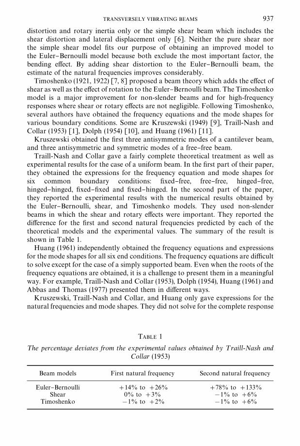
Traill-Nash and Collar gave a fairly complete theoretical treatment as well asexperimental results for the case of a uniform beam. In the "rst part of their paper,they obtained the expressions for the frequency equation and mode shapes forsix common boundary conditions: "xed}free, free}free, hinged}free,hinged}hinged, "xed}"xed and "xed}hinged. In the second part of the paper,they reported the experimental results with the numerical results obtained bythe Euler}Bernoulli, shear, and Timoshenko models. They used non-slenderbeams in which the shear and rotary e!ects were important. They reported thedi!erence for the "rst and second natural frequencies predicted by each of thetheoretical models and the experimental values. The summary of the result isshown in Table 1.
Huang (1961) independently obtained the frequency equations and expressionsfor the mode shapes for all six end conditions. The frequency equations are di$cultto solve except for the case of a simply supported beam. Even when the roots of thefrequency equations are obtained, it is a challenge to present them in a meaningfulway. For example, Traill-Nash and Collar (1953), Dolph (1954), Huang (1961) andAbbas and Thomas (1977) presented them in di!erent ways.
Kruszewski, Traill-Nash and Collar, and Huang only gave expressions for thenatural frequencies and mode shapes. They did not solve for the complete response
TABLE 1
¹he percentage deviates from the experimental values obtained by ¹raill-Nash andCollar (1953)
Beam models First natural frequency Second natural frequency
Euler}Bernoulli #14% to #26% #78% to #133%Shear 0% to #3% !1% to #6%
Timoshenko !1% to #2% !1% to #6%
938 S. M. HAN E¹ A¸.
of the beam due to initial conditions and external forces. To do so, knowledge ofthe orthogonality conditions among the eigenfunctions is required. Theorthogonality conditions for the Timoshenko beam were independently noted byDolph (1954) and Herrmann (1955) [12]. Dolph solved the initial andboundary-value problem for a hinged}hinged beam with no external forces. Themethods used to solve for the forced initial-boundary-value problem and for theproblem with time-dependent boundary conditions are brie#y mentioned in hispaper. A general method to solve for the response of a Timoshenko beam due toinitial conditions and the external forces is given in the book Elastokinetics byReismann and Pawlik (1974) [13]. They used the method of eigenfunctionexpansion.
A crucial parameter in Timoshenko beam theory is the shape factor. It is alsocalled the shear coe$cient or the area reduction factor. This parameter arisesbecause the shear is not constant over the cross-section. The shape factor isa function of Poisson's ratio and the frequency of vibration as well as the shape ofthe cross-section. Typically, the functional dependence on frequency is ignored.Davies (1948) [5], Mindlin and Deresiewicz (1954) [14], Cowper (1966) [15] andSpence and Seldin (1970) [16] suggested methods to calculate the shape factor asa function of the shape of the cross-section and Poisson's ratio. Stephen (1978) [17]showed variation in the shape factor with frequency.
Despite current e!orts (Levinson (1979, 1981) [18}20] to come up with a newand better beam theory, the Euler}Bernoulli and Timoshenko beam theories arestill widely used.
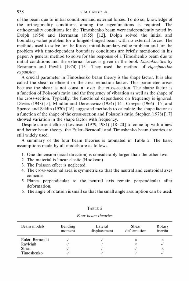
A summary of the four beam theories is tabulated in Table 2. The basicassumptions made by all models are as follows.
1. One dimension (axial direction) is considerably larger than the other two.2. The material is linear elastic (Hookean).3. The Poisson e!ect is neglected.4. The cross-sectional area is symmetric so that the neutral and centroidal axes
coincide.5. Planes perpendicular to the neutral axis remain perpendicular after
deformation.6. The angle of rotation is small so that the small angle assumption can be used.
2. EQUATION OF MOTION AND BOUNDARY CONDITIONS VIAHAMILTON'S PRINCIPLE
2.1. THE EULER}BERNOULLI BEAM MODEL
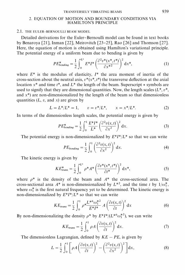
Detailed derivations for the Euler}Bernoulli model can be found in text booksby Benaroya [21], Inman [22], Meirovitch [23}25], Rao [26] and Thomson [27].Here, the equation of motion is obtained using Hamilton's variational principle.The potential energy of a uniform beam due to bending is given by
PE*bending
"
12 P
L*
0
E*I* AL2v*(x*, t*)
Lx*2 B2dx*, (1)
where E* is the modulus of elasticity, I* the area moment of inertia of thecross-section about the neutral axis, v*(x*, t*) the transverse de#ection at the axiallocation x* and time t*, and ¸* the length of the beam. Superscript * symbols areused to signify that they are dimensional quantities. Now, the length scales (¸*, v*,and x*) are non-dimensionalized by the length of the beam so that dimensionlessquantities (¸, v, and x) are given by
¸"¸*/¸*"1, v"v*/¸*, x"x*/¸*. (2)
In terms of the dimensionless length scales, the potential energy is given by
PE*bending
"
12 P
1
0
E*I*¸* A
L2v (x, t)Lx2 B
2dx. (3)
The potential energy is non-dimensionalized by E*I*/¸* so that we can write
PEbending
"
12 P
1
0AL2v(x, t)
Lx2 B2dx. (4)
The kinetic energy is given by
KE*trans
"
12 P
L*
0
o*A* ALv*(x*, t*)
Lt* B2dx*, (5)
where o* is the density of the beam and A* the cross-sectional area. Thecross-sectional area A* is non-dimensionalized by ¸*2, and the time t by 1/u*
1,
where u*1
is the "rst natural frequency yet to be determined. The kinetic energy isnon-dimensionalized by E*I*/¸* so that we can write
KEtrans
"
12 P
1
0
o*¸*6u*2
1E*I*
A ALv(x, t)
Lt B2dx (6)
By non-dimensionalizing the density o* by E*I*/(¸*6u*21
), we can write
KEtrans
"
12 P
1
0
oA ALv (x, t)
Lt B2dx . (7)
The dimensionless Lagrangian, de"ned by KE!PE, is given by
¸"
12 P
1
0CoA A
Lv (x, t)Lt B
2!A
L2v (x, t)Lx2 B
2
D dx , (8)
TRANSVERSELY VIBRATING BEAMS 939
940 S. M. HAN E¹ A¸.
The virtual work due to the non-conservative transverse force per unit lengthf *(x*, t*) is given by
d=*nc"P
L*
0
f *(x*, t*)dv* (x*, t*) dx* . (9)
Non-dimensionalizing the work by E*I*/¸* and the transverse external force f * by¸*3/E*I*, the dimensionless non-conservative work is given by
d=nc"P
1
0
f (x, t)dv(x, t) dx. (10)
Using the extended Hamilton's principle, by including the non-conservativeforcing, the governing di!erential equation of motion is given by
oAL2v(x, t)
Lt2#
L4v(x, t)Lx4
"f (x, t) , (11)
with the boundary conditions to be satis"ed
L2vLx2
d ALvLxB K
1
0
"0,L3vLx3
dv K1
0
"0. (12)
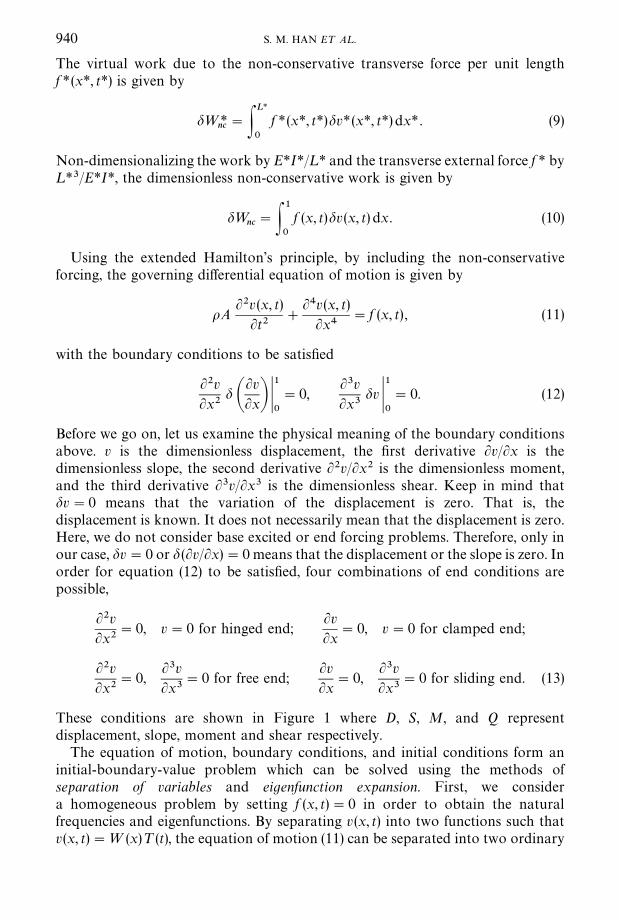
Before we go on, let us examine the physical meaning of the boundary conditionsabove. v is the dimensionless displacement, the "rst derivative Lv/Lx is thedimensionless slope, the second derivative L2v/Lx2 is the dimensionless moment,and the third derivative L3v/Lx3 is the dimensionless shear. Keep in mind thatdv"0 means that the variation of the displacement is zero. That is, thedisplacement is known. It does not necessarily mean that the displacement is zero.Here, we do not consider base excited or end forcing problems. Therefore, only inour case, dv"0 or d(Lv/Lx)"0 means that the displacement or the slope is zero. Inorder for equation (12) to be satis"ed, four combinations of end conditions arepossible,
L2vLx2
"0, v"0 for hinged end;LvLx
"0, v"0 for clamped end;
L2vLx2
"0,L3vLx3
"0 for free end;LvLx
"0,L3vLx3
"0 for sliding end. (13)
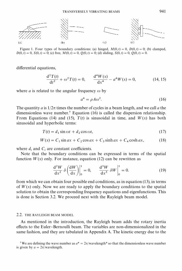
These conditions are shown in Figure 1 where D, S, M, and Q representdisplacement, slope, moment and shear respectively.
The equation of motion, boundary conditions, and initial conditions form aninitial-boundary-value problem which can be solved using the methods ofseparation of variables and eigenfunction expansion. First, we considera homogeneous problem by setting f (x, t)"0 in order to obtain the naturalfrequencies and eigenfunctions. By separating v(x, t) into two functions such thatv(x, t)"= (x)¹(t), the equation of motion (11) can be separated into two ordinary
Figure 1. Four types of boundary conditions: (a) hinged, M(0, t)"0, D (0, t)"0; (b) clamped,D(0, t)"0, S (0, t)"0; (c) free, M(0, t)"0, Q (0, t)"0; (d) sliding, S(0, t)"0, Q(0, t)"0.
TRANSVERSELY VIBRATING BEAMS 941
di!erential equations,
d2¹(t)dt2
#u2¹(t)"0,d4=(x)
dx4!a4=(x)"0, (14, 15)
where a is related to the angular frequency u by
a4"oAu2. (16)
The quantity a is 1/2n times the number of cycles in a beam length, and we call a thedimensionless wave number.s Equation (16) is called the dispersion relationship.From Equations (14) and (15), ¹ (t) is sinusoidal in time, and = (x) has bothsinusoidal and hyperbolic terms:
¹(t)"d1sinut#d
2cosut, (17)
=(x)"C1sin ax#C
2cos ax#C
3sinh ax#C
4cosh ax , (18)
where diand C
iare constant coe$cients.
Note that the boundary conditions can be expressed in terms of the spatialfunction=(x) only. For instance, equation (12) can be rewritten as
d2=dx2
d Ad=dx B K
1
0
"0,d3=dx3
d= K1
0
"0. (19)
from which we can obtain four possible end conditions, as in equation (13), in termsof=(x) only. Now we are ready to apply the boundary conditions to the spatialsolution to obtain the corresponding frequency equations and eigenfunctions. Thisis done is Section 3.2. We proceed next with the Rayleigh beam model.
2.2. THE RAYLEIGH BEAM MODEL
As mentioned in the introduction, the Rayleigh beam adds the rotary inertiae!ects to the Euler}Bernoulli beam. The variables are non-dimensionalized in thesame fashion, and they are tabulated in Appendix A. The kinetic energy due to the
sWe are de"ning the wave number as a*"2n/wavelength* so that the dimensionless wave numberis given by a"2n/wavelength.
942 S. M. HAN E¹ A¸.
rotation of the cross-section is given by
KErot"
12 P
1
0
oI AL2v(x, t)
LtLx B2
dx , (20)
where I* is non-dimensionalized by ¸*4. Combining equation (20) with equations(4), (7) and (10) to form the Lagrangian and using Hamilton's principle, we obtainthe equation of motion given by
oAL2v(x, t)
Lt2#
L4v(x, t)Lx4
!oIL4v (x, t)Lx2Lt2
"f (x, t), (21)
with the boundary conditions given by
L2vLx2
dALvLxB K
1
0
"0, AL3vLx3
!oIL3v
LxLt2Bdv K1
0
"0, (22)
where v is the dimensionless displacement, Lv/Lx the dimensionless slope, L2v/Lx2the dimensionless moment and L3v/Lx3!oI(L3v/LxLt2) the dimensionless shear.Four possible end conditions are
L2vLx2
"0, v"0 for hinged end;LvLx
"0, v"0 for clamped end;
L2vLx2
"0,L3vLx3
!oIL3v
LxLt2"0 for free end;
LvLx
"0,L3vLx3
!oIL3v
LxLt2"0 for sliding end. (23)
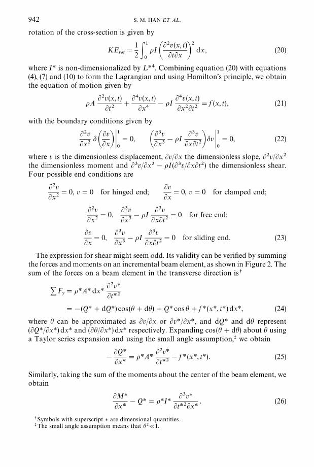
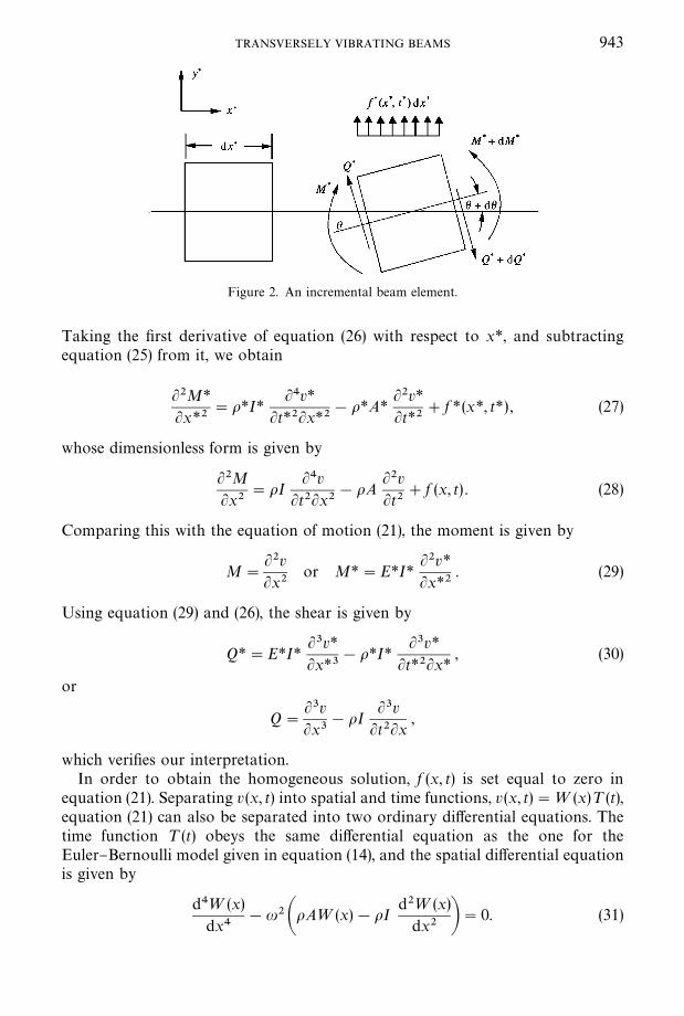
The expression for shear might seem odd. Its validity can be veri"ed by summingthe forces and moments on an incremental beam element, as shown in Figure 2. Thesum of the forces on a beam element in the transverse direction iss
+Fy"o*A*dx*
L2v*Lt*2
"!(Q*#dQ*) cos(h#dh)#Q* cos h#f *(x*, t*) dx*, (24)
where h can be approximated as Lv/Lx or Lv*/Lx*, and dQ* and dh represent(LQ*/Lx*) dx* and (Lh/Lx*) dx* respectively. Expanding cos(h#dh) about h usinga Taylor series expansion and using the small angle assumption,t we obtain
!
LQ*Lx*
"o*A*L2v*Lt*2
!f * (x*, t*). (25)
Similarly, taking the sum of the moments about the center of the beam element, weobtain
LM*Lx*
!Q*"o*I*L3v*
Lt*2Lx*. (26)
sSymbols with superscript * are dimensional quantities.tThe small angle assumption means that h2@1.
Figure 2. An incremental beam element.
TRANSVERSELY VIBRATING BEAMS 943
Taking the "rst derivative of equation (26) with respect to x*, and subtractingequation (25) from it, we obtain
L2M*Lx*2
"o*I*L4v*
Lt*2Lx*2!o*A*
L2v*Lt*2
#f *(x*, t*) , (27)
whose dimensionless form is given by
L2MLx2
"oIL4v
Lt2Lx2!oA
L2vLt2
#f (x, t) . (28)
Comparing this with the equation of motion (21), the moment is given by
M"
L2vLx2
or M*"E*I*L2v*Lx*2
. (29)
Using equation (29) and (26), the shear is given by
Q*"E*I*L3v*Lx*3
!o*I*L3v*
Lt*2Lx*, (30)
or
Q"
L3vLx3
!oIL3v
Lt2Lx,
which veri"es our interpretation.In order to obtain the homogeneous solution, f (x, t) is set equal to zero in
equation (21). Separating v(x, t) into spatial and time functions, v (x, t)"= (x)¹(t),equation (21) can also be separated into two ordinary di!erential equations. Thetime function ¹(t) obeys the same di!erential equation as the one for theEuler}Bernoulli model given in equation (14), and the spatial di!erential equationis given by
d4=(x)dx4
!u2AoA=(x)!oId2=(x)
dx2 B"0. (31)
944 S. M. HAN E¹ A¸.
Again, the time solution ¹ (t) is sinusoidal, and the spatial solution= (x) has bothsinusoidal and hyperbolic terms,
¹(t)"d1sinut#d
2cosut, (32)
=(x)"C1sin ax#C
2cos ax#C
3sinh bx#C
4cosh bx , (33)
where the dispersion relations are
a"JoIu2/2#J(oIu2/2)2#oAu2 ,
b"J!oIu2/2#J(oIu2/2)2#oAu2 . (34)
Note that there are two wave numbers in this case. It will be shown in Section 3.3that these wave numbers are related only by the slenderness ratio.
The boundary conditions given in equation (22) can be written in terms of=(x)only,
d2=dx2
d Ad=dx B K
1
0
"0, Ad3=dx3
#oIu2d=dx Bd= K
1
0
"0. (35)
2.3. THE SHEAR BEAM MODEL
This model adds the e!ect of shear distortion (but not rotary inertia) to theEuler}Bernoulli model. We introduce new variables a, the angle of rotation of thecross-section due to the bending moment, and b, the angle of distortion due toshear. The total angle of rotation is the sum of a and b and is approximately the "rstderivative of the de#ection,
a (x, t)#b (x, t)"Lv (x, t)/Lx . (36)
Therefore, the potential energy due to bending given in equation (4) is slightlymodi"ed in this case such that
PEbending
"
12 P
1
0ALa(x, t)
Lx B2
dx . (37)
The potential energy due to shear is given by
PE*shear
"
12 P
L
0
k@G*A*ALv* (x*, t*)
Lx*!a (x*, t*)B
2dx*. (38)
Using the dimensionless length scales and the dimensionless potential energyexpressions,
PEshear
"
12 P
L
0
k@G*¸*4
E*I*AA
Lv (x, t)Lx
!a(x, t)B2dx . (39)
Non-dimensionalizing G* by E*I*/¸*4, we can write
PEshear
"
12 P
1
0
k@GAALv (x, t)
Lx!a(x, t)B
2dx , (40)
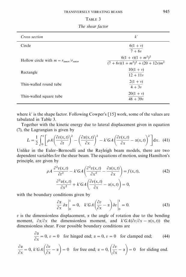
TABLE 3
¹he shear factor
Cross section k@
Circle 6(1#l)7#6l
Hollow circle with m"rinner
/router
6(1#l)(1#m2)2
(7#6l) (1#m2)2#(20#12l)m2
Rectangle10(1#l)12#11l
Thin-walled round tube2(1#l)4#3l
Thin-walled square tube20(1#l)48#39l
TRANSVERSELY VIBRATING BEAMS 945
where k@ is the shape factor. Following Cowper's [15] work, some of the values aretabulated in Table 3.
Together with the kinetic energy due to lateral displacement given in equation(7), the Lagrangian is given by
¸"
12 P
1
0CoAA
Lv(x, t)Lt B
2!A
La(x, t)Lx B
2!k@GAA
Lv (x, t)Lx
!a(x, t)B2
Ddx . (41)
Unlike in the Euler}Bernoulli and the Rayleigh beam models, there are twodependent variables for the shear beam. The equations of motion, using Hamilton'sprinciple, are given by
oAL2v(x, t)
Lt2!k@GAA
L2v(x, t)Lx2
!
La(x, t)Lx B"f (x, t) , (42)
L2a(x, t)Lx2
#k@GAALv (x, t)
Lx!a (x, t)B"0,
with the boundary conditions given by
LaLx
da K1
0
"0, k@GAALvLx
!aB dv K1
0
"0. (43)
v is the dimensionless displacement, a the angle of rotation due to the bendingmoment, La/Lx the dimensionless moment, and k@GA(Lv/Lx!a(x, t)) thedimensionless shear. Four possible boundary conditions are
LaLx
"0, v"0 for hinged end; a"0, v"0 for clamped end; (44)
LaLx
"0, k@GAALvLx
!aB"0 for free end; a"0, ALvLx
!aB"0 for sliding end.
946 S. M. HAN E¹ A¸.
Note that the slope due to the bending moment a is zero (instead of the total slopeLv/Lx) at the clamped or sliding end.
Now, we try to solve the homogeneous problem without the external forcingfunction. The two equations of motion (42) can be decoupled to yield
L4v (x, t)Lx4
!
ok@G
L4v(x, t)Lx2Lt2
#oAL2v (x, t)
Lt2"0,
L4a(x, t)Lx4
!
ok@G
L4a(x, t)Lx2Lt2
#oAL2a(x, t)
Lt2"0. (45)
Note that the forms of the di!erential equations for v and a are identical.sTherefore, we can expect that the forms of v(x, t) and a(x, t) are the same.
The next step is to separate the variables. Here, we "rst assume that they sharethe same time solution ¹(t). In other words, v(x, t) and a (x, t) are synchronized intime,
Cv (x, t)a (x, t)D"¹ (t)C
= (x)W(x) D . (46)
Now, let us substitute the above expression into the governing di!erential equation(42) without the term f (x, t) to obtain
oA=(x)¹G (t)!k@GA(=A(x)!W@ (x))¹(t)"0,
WA(x)¹ (t)#k@GA(=@(x)!W (x))¹ (t)"0, (47)
where the prime and dot notations are used for the derivatives with respect to x andt respectively. The "rst expression in equation (47) can be separated into twoordinary di!erential equations given by
¹G (t)#u2¹(t)"0,
k@GA(=A (x)!W@ (x) )#u2oA=(x)"0. (48)
Again, ¹(t) is sinusoidal with angular frequency u as in equation (17). The spatialequations, the second in equation (47) and the second in equation (48), are writtenusing matrix notation as
0"Ck@GA
001DC=A (x)WA(x) D#C
0k@GA
!k@GA0 D C
=@(x)W@ (x) D
#CoAu2
00
!k@GAD C= (x)W(x) D . (49)
These equations can be decoupled to yield
=@@@@(x)#ou2
k@G=A(x)!oAu2=(x)"0,
W@@@@(x)#ou2
k@GWA (x)!oAu2W(x)"0. (50)
sThe equations can be decoupled in this way only when the cross-sectional area and the density areuniform.
TRANSVERSELY VIBRATING BEAMS 947
Note that the di!erential equations for= (x) and W(x) have the same form, so thatwe can further assume that the solutions of= (x) and W (x) also have the same formand only di!er by a constant as
C= (x)W(x) D"duerx, (51)
where d is the constant coe$cient, u a vector of constant numbers and r the wavenumber.
When equation (51) is substituted into equation (49), we obtain
Ck@GAr2#oAu2
k@GAr!k@GArr2!k@GADu"0, (52)
from which we obtain the eigenvalues r and eigenvectors u. In order to havea non-trivial solution, the determinant of the above matrix has to be zero, that is,
r4#ou2
k@Gr2!oAu2"0. (53)
The eigenvalues are given by
ri"$S!
ou2
2k@G$SA
ou2
2k@GB2#oAu2 for i"1, 2, 3, 4, (54)
of which two are real and the other two are imaginary. The correspondingdimensionless eigenvectors u
iare given by
ui"C
k@GAri
k@GAr2i#oAu2D or C
r2i!k@GA
!k@GAriD . (55)
The spatial solution is given by
C=(x)W(x) D"
4+i/1
diuierix
"d1u1ebx#d
2u2e~bx#d
3u3e*ax#d
4u4e~*ax, (56)
where
a"Sou2
2k@G#SA
ou2
2k@GB2#oAu2 , b"S!
ou2
2k@G#SA
ou2
2k@GB2#oAu2 .
(57)
We can write the spatial solution (56) in terms of the sinusoidal and hyperbolicfunctions with real arguments,
C=(x)W(x) D"C
C1
D1D sin ax#C
C2
D2Dcos ax#C
C3
D3D sinh bx#C
C4
D4Dcosh bx. (58)
948 S. M. HAN E¹ A¸.
It may seem that the spatial solution has eight unknown constant coe$cients,C
iand D
i, instead of the four that we started with [d
iin equation (56)]. By
expressing the exponential functions erix in equation (56) in terms of sinusoidal andhyperbolic functions, the expressions for the coe$cients C
iand D
iare obtained in
terms of eigenvectors,
CC
1D
1D"(d
3u3!d
4u4) i, C
C2
D2D"d
3u3#d
4u4,
CC
3D
3D"(d
1u1!d
2u2) , C
C2
D2D"d
1u1#d
2u2. (59)
Keeping in mind that d3
and d4
are complex conjugates of each other, we obtain
D1"!
k@GAa2!oAu2
k@GAaC
2, D
2"
k@GAa2!oAu2
k@GAaC
1,
D3"
k@GAb2#oAu2
k@GAbC
4, D
4"
k@GAb2#oAu2
k@GAbC
3. (60)
Therefore, there are four unknowns. These relations can be obtained moreeasily by substituting the assumed solution (58) into the spatial di!erentialequations (49).
The boundary conditions in equation (43) are written in terms of spatial solutionsas
dWdx
dW K1
0
"0, k@GAAd=dx
!WBd= K1
0
"0. (61)
2.4. THE TIMOSHENKO BEAM MODEL
Timoshenko proposed a beam theory which adds the e!ects of shear distortionand rotary inertia [7, 8] to the Euler}Bernoulli model.s Therefore, the Lagrangianincludes the e!ects of bending moment (37), lateral displacement (7), rotary inertia(20) and shear distortion (40). We assume that there is no rotational kinetic energyassociated with shear distortion, but only with the rotation due to bending.Therefore, the kinetic energy term used in the Rayleigh beam (20) is modi"ed toinclude only the angle of rotation due to bending by replacing Lv/Lx with a.
Combining modi"ed equation (20) with equations (7), (37) and (40), theLagrangian is given by
¸"
12 P
1
0CoAA
Lv(x, t)Lt B
2#oI A
La(x, t)Lt B
2
!ALa (x, t)
Lx B2!k @GAA
Lv (x, t)Lx
!a(x, t)B2
D dx . (62)
sEquivalently, the Timoshenko model adds rotary inertia to the shear model or adds sheardistortion to the Rayleigh model.
TRANSVERSELY VIBRATING BEAMS 949
The equations of motion are given by
oAL2v(x, t)
Lt2!k@GAA
L2v(x, t)Lx2
!
La(x, t)Lx B"f (x, t) ,
oIL2a(x, t)
Lt2!
L2a(x, t)Lx2
!k@GA ALv(x, t)
Lx!a (x, t)B"0, (63)
and the boundary conditions are given by
LaLx
da K1
0
"0, k@GAALvLx
!aB dv K1
0
"0, (64)
which are identical to those of the shear beam.In order to solve the homogeneous problem, the forcing function is set to zero.
The equations of motion (63) can be decoupled into
L4vLx4
!AoI#o
k@GBL4v
Lx2Lt2#oA
L2vLt2
#
o2Ik@G
L4vLt4
"0,
L4aLx4
!AoI#o
k@GBL4a
Lx2Lt2#oA
L2aLt2
#
o2Ik@G
L4aLt4
"0, (65)
where it is implied that v and a are functions of x and t. Again, both v(x, t) and a(x, t)obey di!erential equations of the same form, so that we can make the sameargument as we did for the shear beam that v (x, t) and a(x, t) themselves are of thesame form.
First, we use the method of separation of variables to separate the equations ofmotion (63) to obtain the time and the spatial ordinary di!erential equations. Thetime equation is the same as the ones for the other models given in equation (14),and the spatial equation is given by
0"Ck@GA
001DC=A (x)WA(x) D#C
0k@GA
!k@GA0 D C
=@(x)W@ (x) D
#CoAu2
00
Ju2!k@GAD C= (x)W (x) D . (66)
Following the procedure used previously from equations (46)} (53), we obtain thecharacteristic equation
r4#AoI#o
k@GBu2r2!oAu2#o2Ik@G
u4"0, (67)
whose roots are
r"$S!AI#1
k@GBou2
2$SAI!
1k@GB
2 o2u4
4#oAu2 . (68)
950 S. M. HAN E¹ A¸.
Of the four roots, the two given by
r1,2
"$S!AI#1
k@GBou2
2!SAI!
1k@GB
2 o2u4
4#oAu2
are always imaginary, and the other two roots given by
r3,4
"$S!AI#1
k@GBou2
2#SAI!
1k@GB
2 o2u4
4#oAu2 (69)
are either real or imaginary depending on the frequency u (for a given material andgeometry). They are real when the frequency is less than Jk@GA/oI and areimaginary when the frequency is greater than Jk@GA/oI. We call this cuto!frequency the critical frequency u
c. Therefore, we must consider two cases when
obtaining spatial solutions: u(ucand u'u
c.
When u(uc, the spatial solution is written in terms of both sinusoidal and
hyperbolic terms,
C=(x)W(x) D"C
C1
D1D sin ax#C
C2
D2D cos ax#C
C3
D3D sinh bx#C
C4
D4D cosh bx , (70)
where
a"SAI# 1k@GB
ou2
2#SAI!
1k@GB
2 o2u4
4#oAu2 ,
b"S!AI#1
k@GBou2
2#SAI!
1k@GB
2 o2u4
4#oAu2 . (71)
and Ciand D
iare related by equation (60).
When u'uc, the spatial solution only has sinusoidal terms,
C= (x)W(x) D"C
CI1
D31D sin ax#C
CI2
D32D cos ax#C
CI3
D33D sin bJ x#C
CI4
D34D cos bJ x , (72)
where
a"SAI# 1k@GB
ou2
2#SAI!
1k@GB
2 o2u4
4#oAu2 ,
bJ "SAI# 1k@GB
ou2
2!SAI!
1k@GB
2 o2u4
4#oAu2 , (73)
and CIiand D3
iare related by
D31"!
k@GAa2!oAu2
k@GAaCI
2, D3
2"
k@GAa2!oAu2
k@GAaCI
1,
D33"!
k@GAbJ 2!oAu2
k@GAbJCI
4, D3
4"
k@GAbJ 2!oAu2
k@GAbJCI
3, (74)
TRANSVERSELY VIBRATING BEAMS 951
Notice that b and bJ are related by
b"ibJ . (75)
Let us examine the frequency and the wave number where the transition occurs.This critical frequency can be written as
uc"S
k@GAoI
"
1k S
k@Go
, (76)
where k is the dimensionless radius of gyration or the inverse of the slendernessratio,
k"SI*A*
1¸*
"
1s
. (77)
By substituting equation (76) into equations (71) and (73), the critical wave numbersare
ac"
1k
J(k@GI#1), bc"bJ
c"0. (78)
Writing in terms of dimensional variables
ac"
1k SAk@
G*E*
#1B"1k SA
1c2#1B , (79)
where c is given bys
c2"E*
k@G*"
2(1#l)k@
. (81)
Recall that k@ depends on the Poisson ratio and the shape of the cross-section. Bothk@ and l do not vary much so that we can say that the critical wave numberessentially depends on the slenderness ratio.
Also, the case when u(ucis equivalent to the case when a(a
c. This can be
veri"ed by taking a derivative of a in the dispersion relationship [equations (71) or(73)] with respect to u. We will "nd that the derivative is always positive implyingthat a is a monotonically increasing function of u.
3. NATURAL FREQUENCIES AND MODE SHAPES
So far, we have obtained the spatial solutions with four unknowns [equations(18) for the Euler}Bernoulli and Rayleigh models, equations (58) with equation (60)for the shear and the Timoshenko models for u(u
c, and equation (72) with
equation (74) for the Timoshenko model for u'uc], and we have identi"ed the
possible boundary conditions that the spatial solutions have to satisfy equation (19)
sHere, we use
G*"E*/2(1#l). (80)
952 S. M. HAN E¹ A¸.
for the Euler}Bernoulli, equation (35) for the Rayleigh and equation (61) for theshear and Timoshenko models]. The next step is to apply a set of boundaryconditions in order to obtain the four unknown coe$cients in the spatial solution.Upon applying the boundary conditions, we obtain four simultaneous equationswhich can be written as
[F]4]4
MCN4]1
"M0N4]1
, (82)
where MCN is the vector of coe$cients in the spatial solution, and the matrix [F]typically has sinusoidal and hyperbolic functions evaluated at the end points. Thedeterminant of [F] has to be zero to avoid the trivial solution or MCN"0. At thispoint, the best we can do is to reduce the number of unknowns from four to one.The equation obtained by setting the determinant to zero is the frequency equation,which has an in"nite number of roots. For each root, the coe$cients C
iof the
corresponding spatial solution are unique only to a constant. The roots are in theform of dimensionless wave numbers, which can be translated into naturalfrequencies using the dispersion relationships. The corresponding spatial solutionsare called the eigenfunctions or the mode shapes. The remaining constant in theeigenfunction is usually determined by normalizing the modal equation forconvenience.s In this section, for each model, we obtain the frequency equations,their roots and the mode shapes for four of the ten boundary conditions. Those forthe other six cases are obtained using the symmetric and antisymmetric modes.
3.1. SYMMETRIC AND ANTISYMMETRIC MODES
First, let us identify all 10 cases. They are free}free, hinged}hinged, clamped}clamped, clamped}free, sliding}sliding, free}hinged, free}sliding, clamped}hinged,clamped}sliding and hinged}sliding supports. Using the symmetric andantisymmetric modes, we try to minimize the cases to be considered.
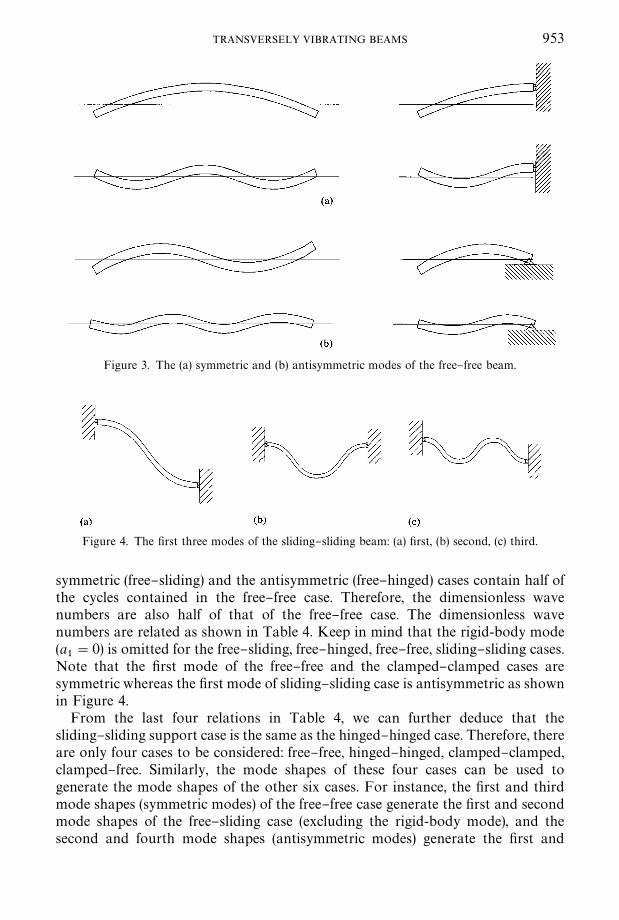
Excluding the rigid-body mode, the free}sliding is the symmetric modet and thefree}hinged is the antisymmetric mode of the free}free case as shown in Figure 3.
Similarly, the clamped}sliding is the symmetric mode and the clamped}hinged isthe antisymmetric mode of the clamped}clamped case. The hinged}sliding is thesymmetric mode of the hinged}hinged case and the antisymmetric mode of thesliding}sliding case.
Once we obtain the dimensionless wave numbers of the free}free, hinged}hinged,clamped}clamped, and clamped}free cases, we can "nd the dimensionless wavenumbers of the remaining cases using the de"nition of the dimensionless wavenumber. The dimensionless wave number is 1/2n times the number of cyclescontained in the beam length. As shown in Figure 3 for the free}free beam, the
ssee sections 5.1 and 5.2 for normalization process.tThe symmetric mode of the free}free beam requires that the total slope of the beam v@ (x, t) in the
middle of the beam is zero. On the other hand, for the shear and Timoshenko models, the free}slidingbeam requires that the angle of rotation due to bending a is zero at the sliding end. It seems that thesymmetric mode of the free}free beam cannot represent the free}sliding beam. However, if we lookmore closely, the other condition for the sliding end is that b"0 which leads to v@"0. Therefore, thefree}sliding beam can be replaced by the symmetric mode of the free}free beam.
Figure 3. The (a) symmetric and (b) antisymmetric modes of the free}free beam.
Figure 4. The "rst three modes of the sliding}sliding beam: (a) "rst, (b) second, (c) third.
TRANSVERSELY VIBRATING BEAMS 953
symmetric (free}sliding) and the antisymmetric (free}hinged) cases contain half ofthe cycles contained in the free}free case. Therefore, the dimensionless wavenumbers are also half of that of the free}free case. The dimensionless wavenumbers are related as shown in Table 4. Keep in mind that the rigid-body mode(a
1"0) is omitted for the free}sliding, free}hinged, free}free, sliding}sliding cases.
Note that the "rst mode of the free}free and the clamped}clamped cases aresymmetric whereas the "rst mode of sliding}sliding case is antisymmetric as shownin Figure 4.
From the last four relations in Table 4, we can further deduce that thesliding}sliding support case is the same as the hinged}hinged case. Therefore, thereare only four cases to be considered: free}free, hinged}hinged, clamped}clamped,clamped}free. Similarly, the mode shapes of these four cases can be used togenerate the mode shapes of the other six cases. For instance, the "rst and thirdmode shapes (symmetric modes) of the free}free case generate the "rst and secondmode shapes of the free}sliding case (excluding the rigid-body mode), and thesecond and fourth mode shapes (antisymmetric modes) generate the "rst and
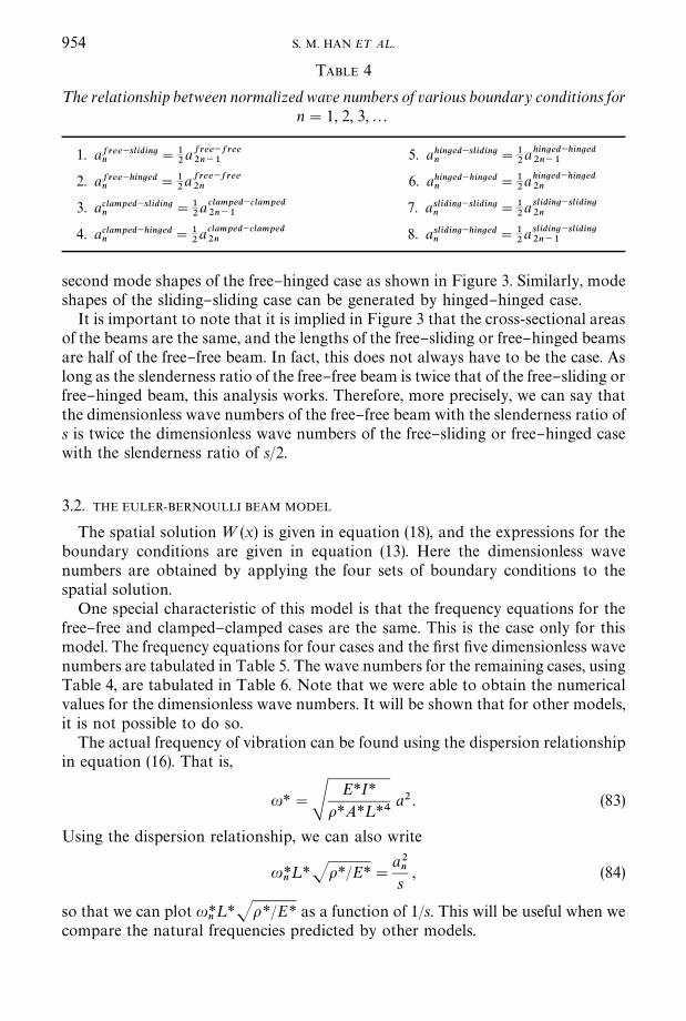
TABLE 4
¹he relationship between normalized wave numbers of various boundary conditions forn"1, 2, 3,2
1. afree~slidingn
"12afree~free2n~1
5. ahinged~slidingn
"12ahinged~hinged2n~1
2. afree~hingedn
"12afree~free2n
6. ahinged~hingedn
"12ahinged~hinged2n
3. aclamped~slidingn
"12a clamped~clamped2n~1
7. asliding~slidingn
"12a sliding~sliding2n
4. aclamped~hingedn
"12aclamped~clamped2n
8. asliding~hingedn
"12asliding~sliding2n~1
954 S. M. HAN E¹ A¸.
second mode shapes of the free}hinged case as shown in Figure 3. Similarly, modeshapes of the sliding}sliding case can be generated by hinged}hinged case.
It is important to note that it is implied in Figure 3 that the cross-sectional areasof the beams are the same, and the lengths of the free}sliding or free}hinged beamsare half of the free}free beam. In fact, this does not always have to be the case. Aslong as the slenderness ratio of the free}free beam is twice that of the free}sliding orfree}hinged beam, this analysis works. Therefore, more precisely, we can say thatthe dimensionless wave numbers of the free}free beam with the slenderness ratio ofs is twice the dimensionless wave numbers of the free}sliding or free}hinged casewith the slenderness ratio of s/2.
3.2. THE EULER-BERNOULLI BEAM MODEL
The spatial solution= (x) is given in equation (18), and the expressions for theboundary conditions are given in equation (13). Here the dimensionless wavenumbers are obtained by applying the four sets of boundary conditions to thespatial solution.
One special characteristic of this model is that the frequency equations for thefree}free and clamped}clamped cases are the same. This is the case only for thismodel. The frequency equations for four cases and the "rst "ve dimensionless wavenumbers are tabulated in Table 5. The wave numbers for the remaining cases, usingTable 4, are tabulated in Table 6. Note that we were able to obtain the numericalvalues for the dimensionless wave numbers. It will be shown that for other models,it is not possible to do so.
The actual frequency of vibration can be found using the dispersion relationshipin equation (16). That is,
u*"SE*I*
o*A*¸*4a2 . (83)
Using the dispersion relationship, we can also write
u*n¸*Jo*/E*"
a2ns
, (84)
so that we can plot u*n¸*Jo*/E* as a function of 1/s. This will be useful when we
compare the natural frequencies predicted by other models.
TABLE 5
¹he frequency equations and the ,rst ,ve wave numbers of Euler}Bernoulli model
The frequency equation a1
a2
a3
a4
a5
c-c and f-f cos a cosh a!1"0 4)730 7)853 10)996 14)137 17)279h-h or s-s sin a sinh a"0 n 2n 3n 4n 5nc-f cos a cosh a#1"0 1)875 4)694 7)855 10)996 14)137
TABLE 6
¹he ,rst ,ve wave numbers obtained using the symmetric and antisymmetric modes
a1
a2
a3
a4
a5
c-s and f-s 2)365 5)498 8)639 11)781 14)923c-h and f-h 3)927 7)069 10)210 13)352 16)493h-s 0)5n 1)5n 2)5n 3)5n 4)5n
TRANSVERSELY VIBRATING BEAMS 955
3.3. THE RAYLEIGH BEAM MODEL
The expressions for the boundary conditions are given in equation (23). Unlike inthe Euler}Bernoulli beam case, there are two wave numbers in the Rayleigh beam,a and b.s The frequency equation will have both a and b. In order to "nd thesolution to the frequency equations, one of the wave numbers has to be expressed interms of the other so that the frequency equation is a function of one wave numberonly, let us say a. Following is the procedure used to express b in terms of a.
The dispersion relations given in equation (34) can be written as
a2"B1#JB2
1#B
2, b2"!B
1#JB2
1#B
2, (85)
where B1
and B2, in this case, are
B1"
oIu2
2, B
2"oAu2 . (86)
Solving for B1
and B2
in equation (85) we obtain
B1"(a2!b2)/2, B
2"a2b2 (87)
Note that equations (87) are still the dispersion relations. Now, let us examine theratio of B
1to B
2. From equations (87) and (86),
B1
B2
"
12 A
1b2
!
1a2B"
I2A
, (88)
sNote that the wave number of a hyperbolic function, b, does not have a physical meaning while thewave number of a sinusoidal function, a, does. Nonetheless, we call b the wave number of thehyperbolic function.
TABLE 7
¹he frequency equations of the Rayleigh model
f-f (b6!a6)sin a sinh b#2a3b3 cos a cosh b!2a3b3"0c-c (b2!a2 ) sin a sinh b!2ab cos a cosh b#2ab"0
h-h or s-s sin a sinh b"0c-f (b2!a2)ab sin a sinh b#(b4#a4) cos a cosh b#2a2b2"0
956 S. M. HAN E¹ A¸.
where the ratio of I to A is k2 from equation (77). Now, we can write
1b2
!
1a2
"k2"1s2
. (89)
Therefore, the wave numbers of the Rayleigh beam are related by the slendernessratio. This contrasts with the case of the Euler}Bernoulli beam where thedimensionless wave numbers are independent of the geometry of the beambut dependent solely on the boundary conditions. Expressing b in terms of a andk (or s),
b"aS1
a2k2#1"asS
1a2#s2
. (90)
Let us consider the case when k"0. Then, a equals b by equation (89) or (90), andB1
is zero by equation (87). Comparing equation (85) with equation (16), we also"nd that the wave numbers a and b are equal to the wave number of theEuler}Bernoulli beam. For a slender beam where s is large (k is small), the two wavenumbers approach each other so that the result resembles that of theEuler}Bernoulli beam.s
The frequency equations for four cases are given in Table 7. Notice that thefrequency equations contain both a and b as predicted earlier. Further, notice thatwhen b is expressed in terms of a using equation (90), the geometrical property,slenderness ratio, enters the frequency equations. Therefore, the roots of thefrequency equations depend on the slenderness of the beam and are no longerindependent of the geometry of the beam. The signi"cance of the previousstatement is that it implies that the mode shapes also vary with the slendernessratio.
As mentioned earlier, as s approaches in"nity, the frequency equation becomesidentical to that of the Euler}Bernoulli beam. The best way to represent thesolution of the frequency equation is to plot wave numbers as a continuousfunction of s or k. Here, we will use k for a reason which will become apparentshortly. The frequency equations in Table 7 are transcendental equations that haveto be solved numerically. In order to obtain a smooth function, a (k), we use thefollowing analysis. Let one of the frequency equations be F(a, b). From equation
sIn general, the slenderness ratio of 100 is su$cient so that there is little di!erence among all fourmodels (Euler}Bernoulli, Rayleigh, shear and Timoshenko).
TRANSVERSELY VIBRATING BEAMS 957
(90), b is a function of a and k, b(a, k). dF and db are given by
dF"
LFLa
da#LFLb
db , db"LbLa
da#LbLk
dk . (91)
Combining two expressions, dF is given by
dF"
LFLa
da#LFLb A
LbLa
da#LbLk
dkB"0, (92)
where dF is zero because F is zero. Solving for da/dk, we obtain
dadk
"
!(LF/Lb)(Lb/Lk)(LF/La)#(LF/Lb)(Lb/La)
, (93)
where the right-hand side is a function of a, b and k. After b is expressed in terms ofa and k by equation (90), the right-hand side is a function of a and k only. Now, thisis a "rst order ordinary di!erential equation which can be solved once we know theinitial value a(k"0). The initial value is identical to the wave numbers of theEuler}Bernoulli model given in Tables 5 and 6. Note that depending on whichwave number we use as an initial value, a
1, a
2,2, we can track that particular wave
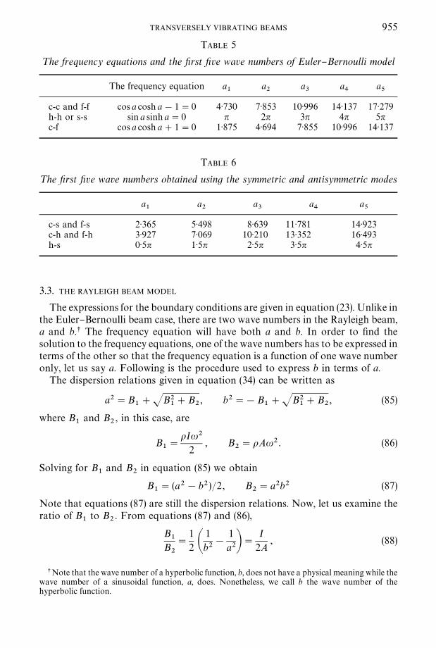
number as the slenderness ratio varies. The initial value problem is solved usingMATLAB, and the results are shown in Figures 5}8. The four solid lines in each"gure are the wave numbers obtained using the Euler}Bernoulli theory. They arenot a!ected by the slenderness ratio. The two lines (dotted and dot-dashed) thatemerge from nth solid line near 1/s"0 are the nth waves numbers, a and b , of the
n n
Figure 5. The "rst four pairs of wave numbers of the free}free Rayleigh beam and clamped}clamped shear beam: * , Euler}Bernoulli; 2, a; } )} )} , b.
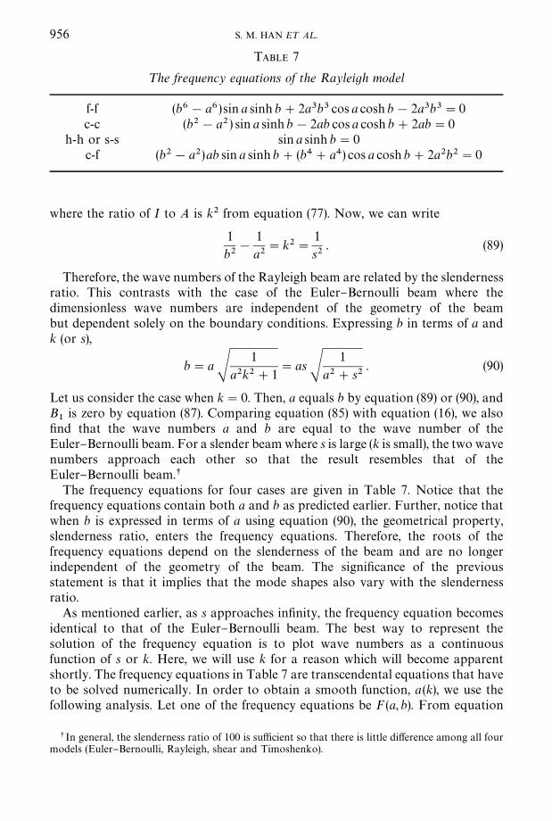
Figure 6. The "rst four pairs of wave numbers of the clamped}clamped Rayleigh beam andfree}free shear beam: * , Euler}Bernoulli; 2, a; } )} )} , b.
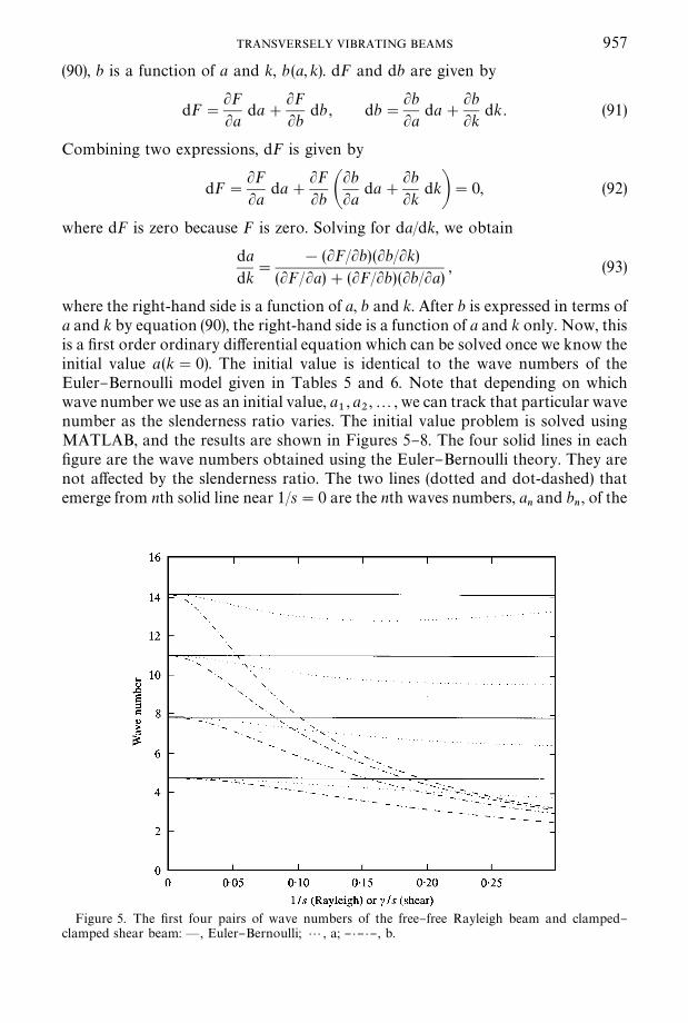
Figure 7. The "rst four pairs of wave numbers of the hinged}hinged (or sliding}sliding) Rayleighand shear beam: * , Euler}Bernoulli or a; } )} )} , b.
958 S. M. HAN E¹ A¸.
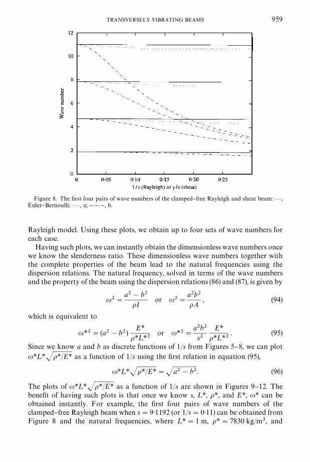
Figure 8. The "rst four pairs of wave numbers of the clamped}free Rayleigh and shear beam:* ,Euler}Bernoulli; 2, a; } )} )} , b.
TRANSVERSELY VIBRATING BEAMS 959
Rayleigh model. Using these plots, we obtain up to four sets of wave numbers foreach case.
Having such plots, we can instantly obtain the dimensionless wave numbers oncewe know the slenderness ratio. These dimensionless wave numbers together withthe complete properties of the beam lead to the natural frequencies using thedispersion relations. The natural frequency, solved in terms of the wave numbersand the property of the beam using the dispersion relations (86) and (87), is given by
u2"a2!b2
oIor u2"
a2b2
oA, (94)
which is equivalent to
u*2"(a2!b2)E*
o*¸*2or u*2"
a2b2
s2E*
o*¸*2. (95)
Since we know a and b as discrete functions of 1/s from Figures 5}8, we can plotu*¸*Jo*/E* as a function of 1/s using the "rst relation in equation (95),
u*¸*Jo*/E*"Ja2!b2. (96)
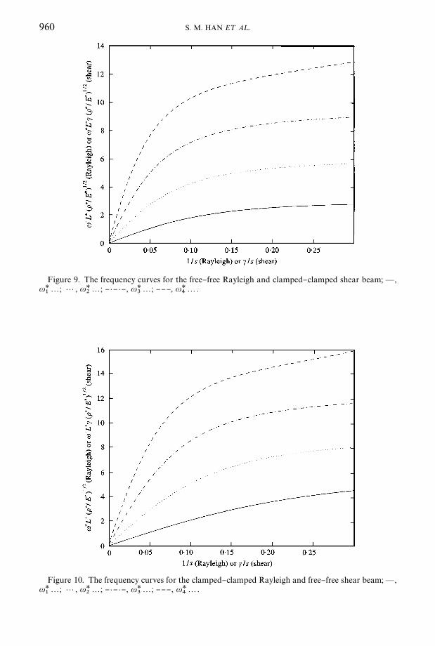
The plots of u*¸*Jo*/E* as a function of 1/s are shown in Figures 9}12. Thebene"t of having such plots is that once we know s, ¸*, o*, and E*, u* can beobtained instantly. For example, the "rst four pairs of wave numbers of theclamped}free Rayleigh beam when s"9)1192 (or 1/s"0)11) can be obtained fromFigure 8 and the natural frequencies, where ¸*"1 m, o*"7830 kg/m3, and
Figure 9. The frequency curves for the free}free Rayleigh and clamped}clamped shear beam; * ,u*
12; 2, u*
22; } )} )} , u*
32; }}}, u*
42.
Figure 10. The frequency curves for the clamped}clamped Rayleigh and free}free shear beam;* ,u*
12; 2, u*
22; } )} )} , u*
32; }}} , u*
42.
960 S. M. HAN E¹ A¸.
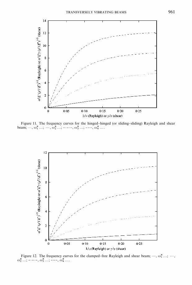
Figure 11. The frequency curves for the hinged}hinged (or sliding}sliding) Rayleigh and shearbeam; * , u*
12; 2, u*
22; } )} )} , u*
32; }}} , u*
42.
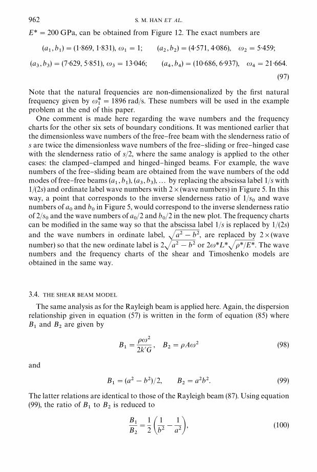
Figure 12. The frequency curves for the clamped}free Rayleigh and shear beam; * , u*12
; 2,u*
22; } )} )} , u*
32; }}} , u*
42.
TRANSVERSELY VIBRATING BEAMS 961
962 S. M. HAN E¹ A¸.
E*"200 GPa, can be obtained from Figure 12. The exact numbers are
(a1, b
1)"(1)869, 1)831), u
1"1; (a
2, b
2)"(4)571, 4)086), u
2"5)459;
(a3, b
3)"(7)629, 5)851), u
3"13)046; (a
4, b
4)"(10)686, 6)937), u
4"21)664.
(97)
Note that the natural frequencies are non-dimensionalized by the "rst naturalfrequency given by u*
1"1896 rad/s. These numbers will be used in the example
problem at the end of this paper.One comment is made here regarding the wave numbers and the frequency
charts for the other six sets of boundary conditions. It was mentioned earlier thatthe dimensionless wave numbers of the free}free beam with the slenderness ratio ofs are twice the dimensionless wave numbers of the free}sliding or free}hinged casewith the slenderness ratio of s/2, where the same analogy is applied to the othercases: the clamped}clamped and hinged}hinged beams. For example, the wavenumbers of the free}sliding beam are obtained from the wave numbers of the oddmodes of free}free beams (a
1, b
1), (a
3, b
3),2 by replacing the abscissa label 1/s with
1/(2s) and ordinate label wave numbers with 2](wave numbers) in Figure 5. In thisway, a point that corresponds to the inverse slenderness ratio of 1/s
0and wave
numbers of a0and b
0in Figure 5, would correspond to the inverse slenderness ratio
of 2/s0and the wave numbers of a
0/2 and b
0/2 in the new plot. The frequency charts
can be modi"ed in the same way so that the abscissa label 1/s is replaced by 1/(2s)and the wave numbers in ordinate label, Ja2!b2, are replaced by 2](wavenumber) so that the new ordinate label is 2Ja2!b2 or 2u*¸*Jo*/E*. The wavenumbers and the frequency charts of the shear and Timoshenko models areobtained in the same way.
3.4. THE SHEAR BEAM MODEL
The same analysis as for the Rayleigh beam is applied here. Again, the dispersionrelationship given in equation (57) is written in the form of equation (85) whereB1
and B2
are given by
B1"
ou2
2k@G, B
2"oAu2 (98)
and
B1"(a2!b2)/2, B
2"a2b2. (99)
The latter relations are identical to those of the Rayleigh beam (87). Using equation(99), the ratio of B
1to B
2is reduced to
B1
B2
"
12 A
1b2
!
1a2B , (100)
TABLE 8
¹he frequency equations of the shear model
f-f (b2!a2)sin a sinh b!2ab cos a cosh b#2ab"0c-c (b6!a6 ) sin a sinh b#2a3b3 cos a cosh b!2a3b3"0
h-h or s-s sin a sinh b"0c-f (b2!a2)ab sin a sinh b#(b4#a4) cos a cosh b#2a2b2"0
TRANSVERSELY VIBRATING BEAMS 963
and using equation (98) the ratio is reduced to
B1
B2
"
12k@GA
"
E*I*¸*2
2k@G*¸*4A*"
(1#l)k@
1s2"
12 A
csB
2, (101)
where c is given in equation (81) and G* is related to E* by equation (80). Therefore,we can write
A1b2
!
1a2B"A
csB
2"(ck)2 . (102)
Solving for b, we obtain
b"aS1
c2k2a2#1"
asc S
1a2#s2/c2
. (103)
Looking again at equation (60), we "nd that the coe$cients in the spatial solutionsare related by
D1"!
b2
aC
2, D
2"
b2
aC
1, D
3"
a2
bC
4, D
4"
a2
bC
3, (104)
so that we can write the spatial solution in terms of the wave numbers only.The frequency equations for the shear beam are given in Table 8. Note that the
frequency equation for the free}free shear beam is identical to the clamped}clamped Rayleigh beam. Also, the frequency equation for the clamped}clampedshear beam is identical to that of the free}free Rayleigh beam. The frequencyequations for the other two cases are the same as the ones for the Rayleigh beam.Also note that the relationship between wave numbers (102) is similar to that of theRayleigh beam (89). In fact, 1/s is modi"ed by the factor c. We can use the plots forthe Rayleigh beam here by just replacing the label for the abscissa 1/s with c/s andswitching the free}free case with the clamped}clamped case. The clamped}clamped case is shown in Figure 5, free}free in Figure 6, hinged}hinged (orsliding}sliding) in Figure 7, and clamped}free in Figure 8.
From equations (98) and (99), the natural frequency is given by
So*¸*2
E* S2(1#l)
k@u*"Ja2!b2 , (105)
where J2(1#l)/k@ is denoted as c throughout this paper as shown in equation(81). Notice the similarity between equations (96) and (105). Therefore, we can use
964 S. M. HAN E¹ A¸.
the plots used in the Rayleigh beam (Figures 9}12) by simply replacing the ordinatewith u*¸*cJo*/E*. The notation u*
n2in the captions are representative of
u*n¸*Jo*/E* for the Rayleigh and u*
n¸*cJo*/E* for the shear model.
Again, these plots are convenient for easily obtaining the natural frequencies fora given s and c. From Figures 8 and 12, for 1/s"0)11, ¸*"1 m, c"2)205,o*"7830 kg/m3, and E*"200 GPa, the pairs of wave numbers and the naturalfrequencies are
(a1, b
1)"(1)846, 1)686), u
1"1; (a
2, b
2)"(4)352, 2)998), u
2"4)1923;
(a3, b
3)"(7)539, 3)626), u
3"8)7823; (a
4, b
4)"(10)686, 3)857), u
4"13)241;
(106)
where the natural frequencies are non-dimensionalized by the "rst naturalfrequency u*
1"1725 rad/s.
3.5. THE TIMOSHENKO BEAM MODEL
Here, we follow the same procedure used for the Rayleigh and the shear beamsby letting
B1"
oIu2
2, B
2"
ou2
2k@G"B
1c2, B
3"oAu2 , (107)
so that the dispersion relations in equations (71) and (73) can be written as
a"J(B1#B
2)#J(B
1!B
2)2#B
3,
b"J!(B1#B
2)#J(B
1!B
2)2#B
3"ibJ . (108)
Solving for B1, B
2and B
3, we obtain
B1"
a2!b2
2(1#c2), B
2"
c2 (a2!b2)2(1#c2)
,
B3"
14 G(a2#b2)2!
(1!c2)2(1#c2)2
(a2!b2)2H , (109)
where c is a constant given in equation (81). Note that B1, B
2, and B
3can be
obtained in terms of a and bJ by replacing b2 with bJ 2 in equation (109). By equatingthe ratio of B
3to B
1using equations (107) and (109), we obtain the relationship
between the wave numbers given by
(c2b2#a2)(a2c2#b2)(a2!b2) (1#c2)
"s2 . (110)
Again, the relationship between a and bJ can be obtained by replacing b with ibJ inequation (110) as
(!c2bJ 2#a2)(c2a2!bJ 2)(a2#bJ 2) (1#c2)
"s2 . (111)
Note that the wave numbers are related by s and c.
TRANSVERSELY VIBRATING BEAMS 965
Using equations (107) and (109), we can write equation (60) as
D1"!
a2#c2b2
(1#c2)aC
2, D
2"
a2#c2b2
(1#c2)aC
1,
D3"
b2#c2a2
(1#c2)bC
4, D
4"
b2#c2a2
(1#c2)bC
3, (112)
so that the spatial solution for u(uccan be written in terms of wave numbers
only. Using equations (107) and (109) with b replaced by ibJ , the coe$cients CIiand
D3iin equation (74) are then related by
D31"!
a2!c2bJ 2(1#c2)a
CI2, D3
2"
a2!c2bJ 2(1#c2)a
CI1,
D33"!
bJ 2!c2a2
(1#c2)bJCI
4, D3
4"
bJ 2!c2a2
(1#c2)bJCI
3, (113)
which we can use to express the spatial solution for u'ucin terms of the wave
numbers only.Note that we only need to obtain one frequency equation for each boundary
condition. Once the frequency equation for the case a(acis obtained, the other
frequency equation for a'accan be obtained by replacing b with ibJ . The frequency
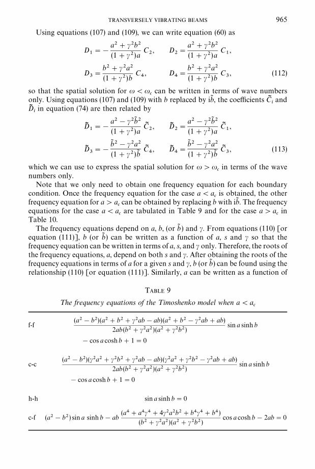
equations for the case a(acare tabulated in Table 9 and for the case a'a
cin
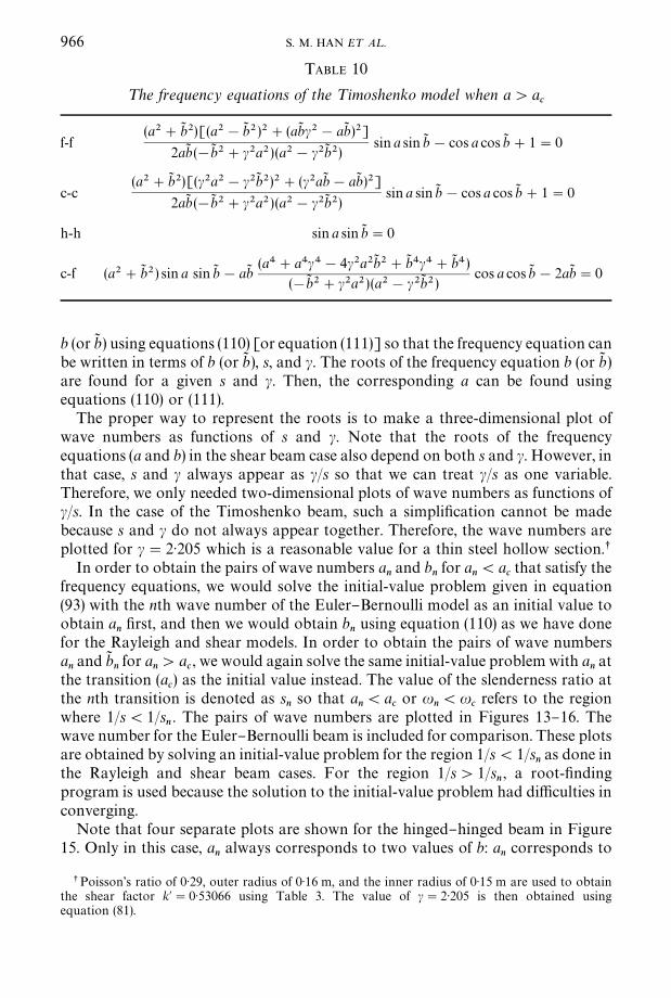
Table 10.The frequency equations depend on a, b, (or bJ ) and c. From equations (110) [or
equation (111)], b (or bJ ) can be written as a function of a, s and c so that thefrequency equation can be written in terms of a, s, and c only. Therefore, the roots ofthe frequency equations, a, depend on both s and c. After obtaining the roots of thefrequency equations in terms of a for a given s and c, b (or bJ ) can be found using therelationship (110) [or equation (111)]. Similarly, a can be written as a function of
TABLE 9
¹he frequency equations of the ¹imoshenko model when a(ac
f-f(a2!b2)(a2#b2#c2ab!ab) (a2#b2!c2ab#ab)
2ab (b2#c2a2) (a2#c2b2)sin a sinh b
!cos a cosh b#1"0
c-c(a2!b2)(c2a2#c2b2#c2ab!ab) (c2a2#c2b2!c2ab#ab)
2ab (b2#c2a2) (a2#c2b2)sin a sinh b
!cos a cosh b#1"0
h-h sin a sinh b"0
c-f (a2!b2) sin a sinh b!ab(a4#a4c4#4c2a2b2#b4c4#b4)
(b2#c2a2)(a2#c2b2)cos a cosh b!2ab"0
TABLE 10
¹he frequency equations of the ¹imoshenko model when a'ac
f-f(a2#bJ 2)[(a2!bJ 2)2#(abJ c2!abJ )2]
2abJ (!bJ 2#c2a2)(a2!c2bJ 2)sin a sin bJ !cos a cos bJ #1"0
c-c(a2#bJ 2)[(c2a2!c2bJ 2)2#(c2abJ !abJ )2]
2abJ (!bJ 2#c2a2)(a2!c2bJ 2)sin a sin bJ !cos a cos bJ #1"0
h-h sin a sin bJ "0
c-f (a2#bJ 2) sin a sin bJ !abJ(a4#a4c4!4c2a2bJ 2#bJ 4c4#bJ 4)
(!bJ 2#c2a2)(a2!c2bJ 2)cos a cos bJ !2abJ "0
966 S. M. HAN E¹ A¸.
b (or bJ ) using equations (110) [or equation (111)] so that the frequency equation canbe written in terms of b (or bJ ), s, and c. The roots of the frequency equation b (or bJ )are found for a given s and c. Then, the corresponding a can be found usingequations (110) or (111).
The proper way to represent the roots is to make a three-dimensional plot ofwave numbers as functions of s and c. Note that the roots of the frequencyequations (a and b) in the shear beam case also depend on both s and c. However, inthat case, s and c always appear as c/s so that we can treat c/s as one variable.Therefore, we only needed two-dimensional plots of wave numbers as functions ofc/s. In the case of the Timoshenko beam, such a simpli"cation cannot be madebecause s and c do not always appear together. Therefore, the wave numbers areplotted for c"2)205 which is a reasonable value for a thin steel hollow section.s
In order to obtain the pairs of wave numbers anand b
nfor a
n(a
cthat satisfy the
frequency equations, we would solve the initial-value problem given in equation(93) with the nth wave number of the Euler}Bernoulli model as an initial value toobtain a
n"rst, and then we would obtain b
nusing equation (110) as we have done
for the Rayleigh and shear models. In order to obtain the pairs of wave numbersanand bJ
nfor a
n'a
c, we would again solve the same initial-value problem with a
nat
the transition (ac) as the initial value instead. The value of the slenderness ratio at
the nth transition is denoted as sn
so that an(a
cor u
n(u
crefers to the region
where 1/s(1/sn. The pairs of wave numbers are plotted in Figures 13}16. The
wave number for the Euler}Bernoulli beam is included for comparison. These plotsare obtained by solving an initial-value problem for the region 1/s(1/s
nas done in
the Rayleigh and shear beam cases. For the region 1/s'1/sn, a root-"nding
program is used because the solution to the initial-value problem had di$culties inconverging.
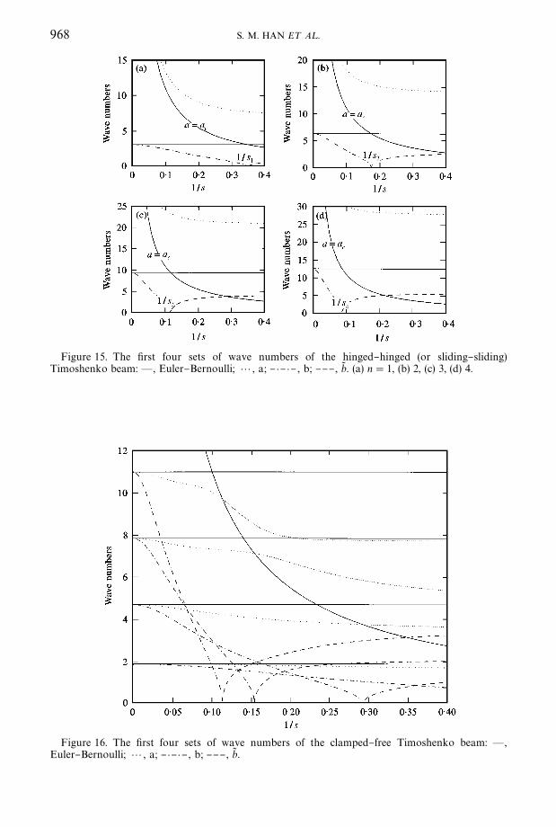
Note that four separate plots are shown for the hinged}hinged beam in Figure15. Only in this case, a
nalways corresponds to two values of b: a
ncorresponds to
sPoisson's ratio of 0)29, outer radius of 0)16 m, and the inner radius of 0)15 m are used to obtainthe shear factor k@"0)53066 using Table 3. The value of c"2)205 is then obtained usingequation (81).
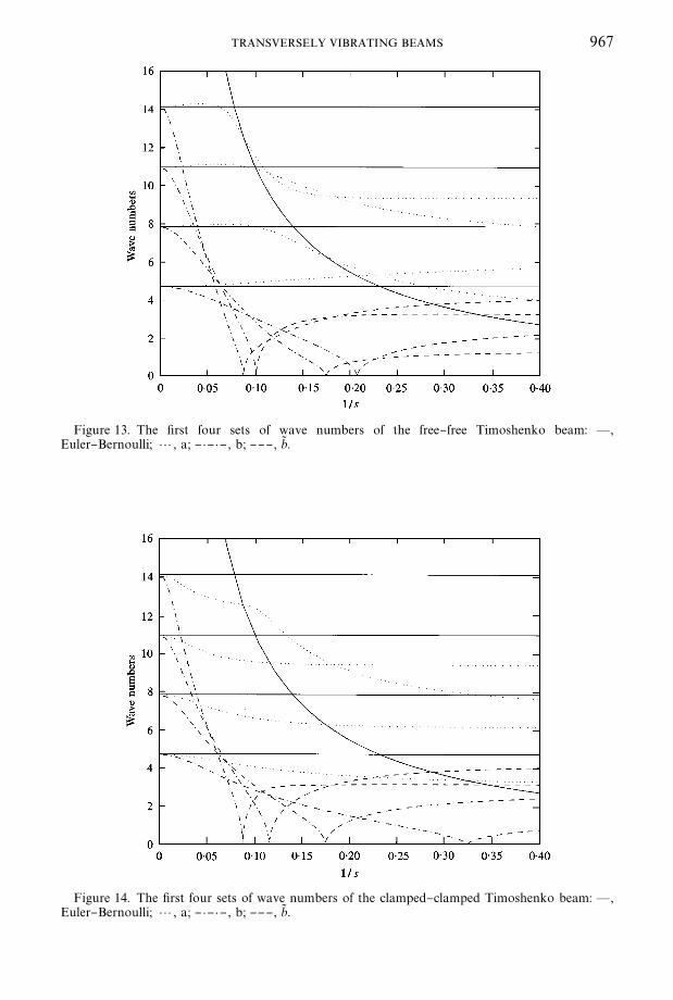
Figure 13. The "rst four sets of wave numbers of the free}free Timoshenko beam: * ,Euler}Bernoulli; 2, a; } )} )} , b; }}} , bJ .
Figure 14. The "rst four sets of wave numbers of the clamped}clamped Timoshenko beam: * ,Euler}Bernoulli; 2, a; } )} )} , b; }}} , bJ .
TRANSVERSELY VIBRATING BEAMS 967
Figure 15. The "rst four sets of wave numbers of the hinged}hinged (or sliding}sliding)Timoshenko beam: * , Euler}Bernoulli; 2, a; } )} )} , b; }}} , bJ . (a) n"1, (b) 2, (c) 3, (d) 4.
Figure 16. The "rst four sets of wave numbers of the clamped}free Timoshenko beam: * ,Euler}Bernoulli; 2, a; } )} )} , b; }}} , bJ .
968 S. M. HAN E¹ A¸.
TRANSVERSELY VIBRATING BEAMS 969
bnand bJ (2)
nfor 1/s(1/s
nand to bJ (1)
nand bJ (2)
nfor 1/s'1/s
n. It is important to note
that each pair corresponds to a distinct natural frequency. The consequence is thatthere are twice as many natural frequencies in the hinged}hinged case as in othercases.
In order to explain why this is the case, let us look at the frequency equation ofthe hinged}hinged beam given in Table 9 or 10.
sin a sinh b"0 for a(ac, sin a sin bJ "0 for a'a
c. (114)
Note that the frequency equation is satis"ed for any value of b (or bJ ) as long assin ax is zero (or a
n"nn for n"1, 2, 3,2). When we solve for b
n(or bJ ) that
corresponds to an
in equation (110) or (111), there are two unique expressions.When 1/s(1/s
n, one is real and the other is imaginary. We call the real root b
nand
the imaginary root ibJ (2)n
. When 1/s'1/sn, both roots are imaginary where one is
ibJ (1)n
and the other is ibJ (2)n
.The natural frequencies that correspond to each pair can be calculated using the
relation for B1
in equations (107) and (109). The natural frequencies for thefree}free, clamped}clamped, and clamped}free cases are given by
u*n¸*Jo*/E*"S
a2n!b2
n1#c2
for 1/s(1/sn
"Sa2n#(bJ
n)2
1#c2for 1/s'1/s
n. (115)
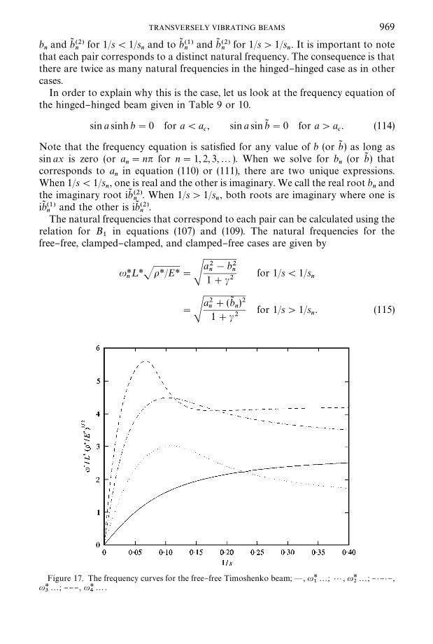
Figure 17. The frequency curves for the free}free Timoshenko beam;* , u*12
; 2, u*22
; } )} )} ,u*
32; }}} , u*
42.
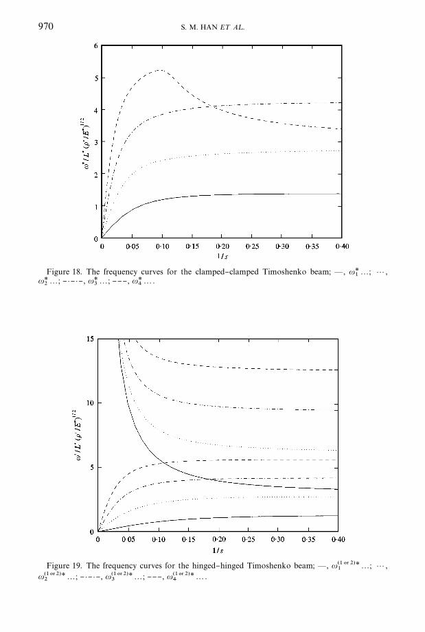
Figure 18. The frequency curves for the clamped}clamped Timoshenko beam; * , u*12
; 2,u*
22; } )} )} , u*
32; }}} , u*
42.
Figure 19. The frequency curves for the hinged}hinged Timoshenko beam; * , u(1 032)*1 2; 2,
u(1032)*2 2; } )} )} , u(1032)*
3 2; }}} , u(1032)*4 2.
970 S. M. HAN E¹ A¸.
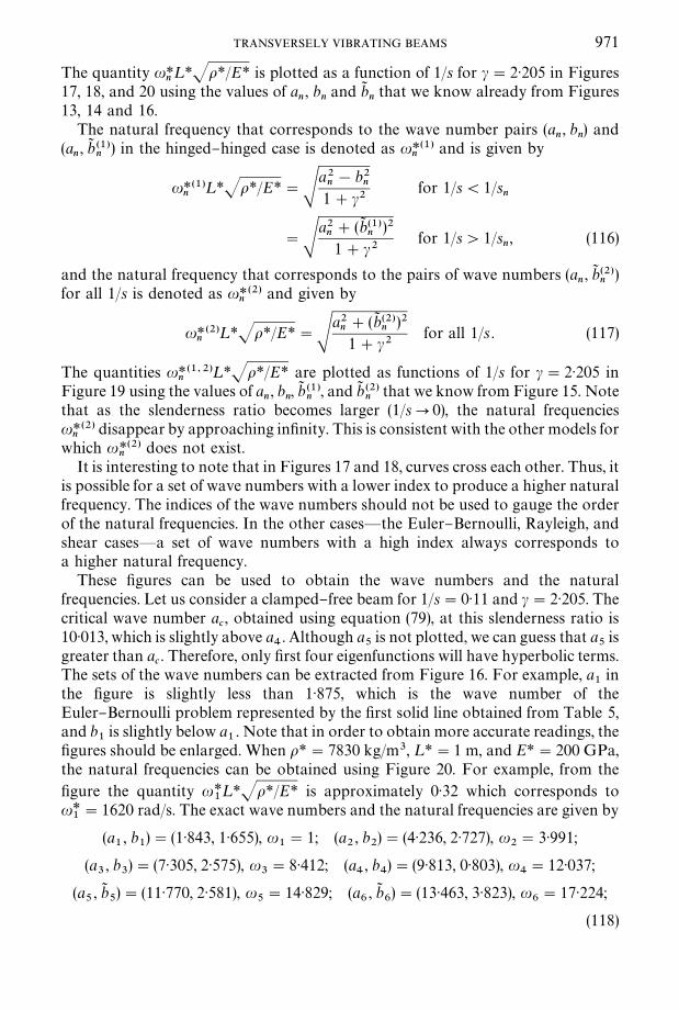
TRANSVERSELY VIBRATING BEAMS 971
The quantity u*n¸*Jo*/E* is plotted as a function of 1/s for c"2)205 in Figures
17, 18, and 20 using the values of an, b
nand bJ
nthat we know already from Figures
13, 14 and 16.The natural frequency that corresponds to the wave number pairs (a
n, b
n) and
(an, bJ (1)
n) in the hinged}hinged case is denoted as u*(1)
nand is given by
u*(1)n
¸*Jo*/E*"Sa2n!b2
n1#c2
for 1/s(1/sn
"Sa2n#(bJ (1)
n)2
1#c2for 1/s'1/s
n, (116)
and the natural frequency that corresponds to the pairs of wave numbers (an, bJ (2)
n)
for all 1/s is denoted as u*(2)n
and given by
u*(2)n
¸*Jo*/E*"Sa2n#(bJ (2)
n)2
1#c2for all 1/s . (117)
The quantities u*(1,2)n
¸*Jo*/E* are plotted as functions of 1/s for c"2)205 inFigure 19 using the values of a
n, b
n, bJ (1)
n, and bJ (2)
nthat we know from Figure 15. Note
that as the slenderness ratio becomes larger (1/sP0), the natural frequenciesu*(2)
ndisappear by approaching in"nity. This is consistent with the other models for
which u*(2)n
does not exist.It is interesting to note that in Figures 17 and 18, curves cross each other. Thus, it
is possible for a set of wave numbers with a lower index to produce a higher naturalfrequency. The indices of the wave numbers should not be used to gauge the orderof the natural frequencies. In the other cases*the Euler}Bernoulli, Rayleigh, andshear cases*a set of wave numbers with a high index always corresponds toa higher natural frequency.
These "gures can be used to obtain the wave numbers and the naturalfrequencies. Let us consider a clamped}free beam for 1/s"0)11 and c"2)205. Thecritical wave number a
c, obtained using equation (79), at this slenderness ratio is
10)013, which is slightly above a4. Although a
5is not plotted, we can guess that a
5is
greater than ac. Therefore, only "rst four eigenfunctions will have hyperbolic terms.
The sets of the wave numbers can be extracted from Figure 16. For example, a1
inthe "gure is slightly less than 1)875, which is the wave number of theEuler}Bernoulli problem represented by the "rst solid line obtained from Table 5,and b
1is slightly below a
1. Note that in order to obtain more accurate readings, the
"gures should be enlarged. When o*"7830 kg/m3, ¸*"1 m, and E*"200 GPa,the natural frequencies can be obtained using Figure 20. For example, from the"gure the quantity u*
1¸*Jo*/E* is approximately 0)32 which corresponds to
u*1"1620 rad/s. The exact wave numbers and the natural frequencies are given by
(a1, b
1)"(1)843, 1)655), u
1"1; (a
2, b
2)"(4)236, 2)727), u
2"3)991;
(a3, b
3)"(7)305, 2)575), u
3"8)412; (a
4, b
4)"(9)813, 0)803), u
4"12)037;
(a5, bJ
5)"(11)770, 2)581), u
5"14)829; (a
6, bJ
6)"(13)463, 3)823), u
6"17)224;
(118)
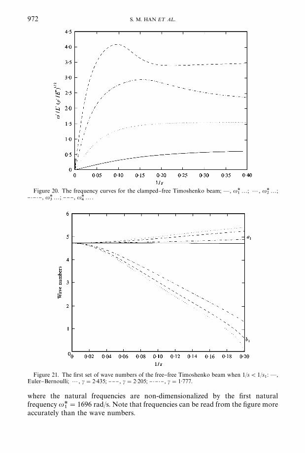
Figure 20. The frequency curves for the clamped}free Timoshenko beam; * , u*12
; 2, u*22
;} )} )} , u*
32; }}} , u*
42.
Figure 21. The "rst set of wave numbers of the free}free Timoshenko beam when 1/s(1/s1: * ,
where the natural frequencies are non-dimensionalized by the "rst naturalfrequency u*
1"1696 rad/s. Note that frequencies can be read from the "gure more
accurately than the wave numbers.
TRANSVERSELY VIBRATING BEAMS 973
Figure 21 shows the variation of the "rst pair of wave numbers (a1, b
1) for
1/s(1/s1
for the free}free Timoshenko beam shown in Figure 13. The values ofc used here are 1)7777, 2)2050 and 2)435. c"1)7777 is a reasonable value for a solidcircular or rectangular section, and c"2)435 is a reasonable value for a thin squaretubes with the Poisson ratio of 0)29.
4. COMPARISONS OF FOUR MODELS
So far, we obtained the wave numbers and natural frequencies of four engineer-ing beam theories. The di!erence among them was the inclusion of di!erent secondorder terms: rotary and shear terms. The Euler}Bernoulli model included only the"rst order terms, translation and bending. The Rayleigh model included therotation, the shear model included the shear and the Timoshenko model includedboth rotation and shear in addition to the "rst order e!ects. In this section, wecompare the relative signi"cance of rotary and shear e!ects and see how it ismanifested in the natural frequency and mode shapes.
The rotary e!ect is represented by the term oI and the shear by o/k@G. Note thatthe shear term is always c2 times larger than the rotary term,
ok@G
"
ok@
E*I*G*¸*4
"
ok@
E*IG*
"oI2(1#l)
k@"oIc2. (119)
Recall that the Poisson ratio l is a physical property that depends on the materialand the shear factor k@ depends on the Poisson ratio and the geometry of thecross-section. The Poisson ratio for a typical metal is about 0)3, and with this value,the shear factor for di!erent cross-sections using, Table 3, ranges from 0)436 for thethin-walled square tube to 0)886 for the circular cross-section. Using these values,c2 ranges from 2)935 for the circular cross-section to 5)96 for the thin-walled squaretube. We have established, for a typical material and cross-section, the shear term isroughly 3}6 times larger than the rotary term.
Now we look into circumstances under which those second order e!ects becomeimportant. Consider the frequency equations obtained previously in Tables 5 and7}10. We observe that the frequency equations for the Euler}Bernoulli modeldepend neither on the geometrical nor the physical properties. Therefore, wavenumber a is independent of any properties. On the other hand, the frequencyequations for the Rayleigh model are functions of a and b which are related by theslenderness ratio s. Therefore, the wave numbers a and b depend on the geometricalproperty s. The frequency equations for the shear and Timoshenko models dependon both s and c. Therefore, the wave numbers depends on both geometrical andphysical properties. The e!ects of s and/or c on the wave numbers are shown inFigures 5}8 for the Rayleigh and shear model and in Figures 13}16 and Figure 21for the Timoshenko model. Generally, the wave numbers deviate from those of
sThe values of c are calculated using the Table 3 and equation (81).
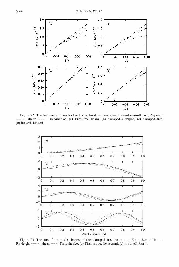
Figure 22. The frequency curves for the "rst natural frequency:* , Euler}Bernoulli; 2, Rayleigh;} )} )} , shear; }}} , Timoshenko. (a) Free}free beam, (b) clamped}clamped, (c) clamped}free,(d) hinged}hinged.
Figure 23. The "rst four mode shapes of the clamped}free beam: * , Euler}Bernoulli; 2,Rayleigh; } )} )} , shear; }}} , Timoshenko. (a) First mode, (b) second, (c) third, (d) fourth.
974 S. M. HAN E¹ A¸.
TRANSVERSELY VIBRATING BEAMS 975
Euler}Bernoulli model as s decreases and c increases. However, the range of c2 ismore restricted (between 3 and 6 for a typical metal and cross-section). Therefore,the wave numbers are strong functions of the slenderness ratio.
As a numerical example, the "rst natural frequencies predicted by each ofthe four models are plotted in Figure 22. The natural frequency is multipliedby ¸*Jo*/E* and c"2)205 is used. The straight solid line for the Euler}Bernoullimodel is obtained using equation (84). Note that the natural frequency predictedby the Euler}Bernoulli model approaches in"nity as the slenderness ratiodecreases whereas the natural frequencies predicted by other models level o!at some point. In Figure 23, the "rst four mode shapes of a clamped}freebeam with s"9)1192 and c"2)205 are plotted. The mode shapes arenormalized with respect to each other for easy comparison. Notice that the naturalfrequencies and mode shapes obtained using the Euler}Bernoulli and Rayleighmodels are similar, and those based on the shear and Timoshenko models aresimilar. This con"rms our result that the shear is more dominant than the rotarye!ects.
In summary, when the slenderness ratio is large (s'100), the Euler}Bernoullimodel should be used. When the slenderness ratio is small, either shear orTimoshenko model can be used.
5. THE FREE AND FORCED RESPONSE
5.1. THE ORTHOGONALITY CONDITIONS FOR THE EULER}BERNOULLI, SHEARAND TIMOSHENKO MODELS
In order to obtain the free or forced response of the beam, we use the methodof eigenfunction expansion. Therefore, the orthogonality conditions of theeigenfunctions have to be established for each beam model. For the modelsdiscussed so far, with the exception of the Rayleigh beam,s the spatial equations ofthe homogeneous problem, (15), (49) and (66) can be written using the operatorformalism
¸(Wn)"u2
nM(W
n) , (120)
where Wn
can denote the nth eigenfunction=n
for the Euler}Bernoulli model, orthe nth vector of eigenfunctions [=
nW
n]T for the shear and Timoshenko models,
and corresponds to the natural frequency u2n
uniquely to within an arbitraryconstant [28, p. 135]. The expressions for the operators for each model are givenbelow.
Euler}Bernoulli model:
¸ (=n)"
d4=n
dx4, M(=
n)"oA=
n. (121)
sThe analysis for the Rayleigh beam is slightly di!erent due to the mixed term in the governingdi!erential equation. It will be discussed in detail in the next section.
976 S. M. HAN E¹ A¸.
Shear model:
¸(Wn)"
k@GAd2
dx2
k@GAddx
!k@GAddx
d2
dx2!k@GA
C=
nW
nD , M (W
n)"C
oA0
00D C=
nW
nD . (122)
¹imoshenko model:
¸(Wn)"
k@GAd2
dx2
k@GAddx
!k@GAddx
d2
dx2!k@GA
C=
nW
nD , M (W
n)"C
oA0
0oID C
=n
WnD . (123)
The operators ¸ and M are self-adjoint (with corresponding boundaryconditions) if [23]
P1
0
[WTn¸(W
m)!WT
m¸(W
n)] dx"0, (124)
P1
0
[WTnM(W
m)!WT
mM(W
n)] dx"0. (125)
Note that the second condition, equation (125), is automatically satis"ed for allthree models. Using equation (120) we can write equation (124) as
(u2m!u2
n) P
1
0
WTnM(W
m) dx"0. (126)
Since eigenvalues (squares of natural frequencies) are unique to the eigenfunctions,u2
mOu2
nfor mOn, in order for above equation to be zero, the integral has to be
zero,
P1
0
WTnM(W
m) dx"0 for mOn. (127)
This is the orthogonality condition for the eigenfunctions. When m"n, wenormalize the eigenfunctions by setting the integral equal to one,
P1
0
WTnM(W
n) dx"1 for n"1, 2, 3,2 (128)
Combining equations (127) and (128), we can write
P1
0
WTnM (W
m) dx"d
nm, (129)
where dnm
is the Kronecker delta.Now we discuss which boundary conditions make the operator ¸ self-adjoint or
satisfy equation (124). The conditions can be found by substituting the expressionfor the operator ¸ into equation (124) and integrating by parts. For example, for the
where the remaining integrals cancel each other due to symmetry. These are theconditions that have to be satis"ed in order for the system to be self-adjoint and theorthogonality condition to hold. Note that the boundary conditions from thevariational problem (19) satisfy this condition.
For the shear and Timoshenko models, the corresponding boundary conditionsfor the self-adjoint operator ¸ are found to be
0"k@GAC=n Ad=
mdx
!WmB!=m A
d=n
dx!W
nBD K1
0
#CWn
dWm
dx!W
m
dWn
dx D K1
0
, (132)
where the boundary conditions obtained from the variational problem (61) alsosatisfy this condition.
Therefore, for the systems we consider, they are self-adjoint and theeigenfunctions are orthogonal to each other as given in equation (127).
5.2. THE ORTHOGONALITY CONDITIONS FOR THE RAYLEIGH MODEL
The spatial equation for the Rayleigh beam (31) can be written in the form givenby equation (120) as was done for the other three models with the operators ¸ andM given by
¸(=n)"
d4=n
dx4, M(=
n)"AoA=
n!oI
d2=n
dx2 B . (133)
However, in this case, the operator M is a di!erential operator unlike those in theother cases. Equation (124), with the operator ¸ substituted with equation (120) isgiven by
P1
0
[=n¸(=
m)!=
m¸(=
n)] dx"P
1
0
[u2m=
nM(=
m)!u2
n=
mM (=
n)] dx . (134)
Substituting the expressions for the ¸ and M operators and integrating by partstwice, the left-hand side of equation (134) is reduced to
A=n
d3=m
dx3!=
m
d3=n
dx3 B K1
0
#A!d=
ndx
d2=m
dx2#
d=m
dxd2=
ndx2 B K
1
0
"0, (135)
978 S. M. HAN E¹ A¸.
where the remaining integrals cancel each other. The right-hand side of equation(134) is reduced to
(u2m!u2
n) P
1
0CoA=
m=
n#oI
d=m
dxd=
ndx D dx!oICu2
m=
n
d=m
dx!u2
n=
m
d=n
dx D K1
0
.
(136)
Combining the left- and right-hand sides equations [(135) and (136)], we obtain
C=nAd3=
mdx3
#oIu2m
d=m
dx B!=m Ad3=
ndx3
#oIu2n
d=n
dx BD K1
0
#A!d=
ndx
d2=m
dx2#
d=m
dxd2=
ndx2 B K
1
0
"(u2m!u2
n) P
1
0CoA=
m=
n#oI
d=m
dxd=
ndx D dx . (137)
Let us examine the left-hand side of equation (137). Comparing with the boundaryconditions from the variational problem, we "nd that the left-hand side vanishes[see equations (35)] so that the orthogonality condition is given by
P1
0CoA=
m=
n#oI
d=m
dxd=
ndx D dx"d
nm. (138)
There are other orthogonality conditions that we can obtain by manipulatingequation (120), where the expressions for the operators are given by equation (133).Multiplying equation (120) by=
mand integrating over the domain (0)x)1), we
obtain
P1
0
=n
d4=m
dx4dx"P
1
0
u2m=
nAoA=m!oI
d2=m
dx2 Bdx , (139)
which can be rewritten as
P1
0
=n
d4=m
dx4dx#u2
moI P
1
0Cd=
ndx
d=m
dx#=
n
d2=m
dx2 Ddx
"u2m P
1
0CoA=
n=
m#oI
d=n
dxd=
mdx D dx , (140)
where the right-hand side equals u2mdnm
from equation (138). We integrate theleft-hand side twice by parts to obtain
=nA
d3=m
dx3#u2
moI
d=m
dx B K1
0
!P1
0
d=n
dxd3=
mdx3
dx"u2mdnm
. (141)
From the boundary conditions (35), the "rst term vanishes and we are left with
!P1
0
d=n
dxd3=
mdx3
dx"u2mdnm
. (142)
TRANSVERSELY VIBRATING BEAMS 979
Integrating equation (142) by parts and using the boundary conditions (35) again,we obtain
P1
0
d2=n
dx2
d2=m
dx2dx"u2
mdnm
. (143)
Therefore, we now have three orthogonality conditions given by equations (138),(142) and (143). The orthogonality condition in equation (142) will be used later.
Note that a similar procedure can be applied to the other models to obtain otherorthogonality conditions.
5.3. THE FREE AND FORCED RESPONSE VIA EIGENF;NC¹ION EXPANSION OF THE
EULER}BERNOULLI, SHEAR, AND TIMOSHENKO MODELS
The method of eigenfunction expansion assumes that the solutions v(x, t) [orsolutions v (x, t) and a (x, t)] to equations of motion given in equations (11), (42), (63)and the forcing function f (x, t) can be represented as a summation of eigenfunctions(the spatial solution to the homogeneous problem) multiplied by functions of timethat are to be determined, that is,
v (x, t)"=+n/1
gn(t)W
n(x), f (x, t)"
=+n/1
Fn(t)M(W
n(x) ). (144, 145)
Note that v (x, t) stands for v(x, t) for the Euler}Bernoulli and Rayleigh models and[v(x, t) a (x, t)]T for shear and Timoshenko models. If we know time-dependentcoe$cients g
n(t), we can solve for the complete solution to the problem as follows.
The expressions for gn(t) can be obtained by applying the operator M to equation
(144) multiplying it by WTm
and integrating over the domain. Simpli"cations can bemade using the orthonormality conditions given in equation (129).
P1
0
WTmM(v (x, t)) dx"
=+n/1
gn(t) P
1
0
WTmM(W
n(x) ) dx . (146)
Therefore,
gn(t)"P
1
0
WTmM(v (x, t) ) dx . (147)
Similarly, Fm(t) can be found by multiplying equation (145) by WT
mand integrating
over the domain,
Fm(t)"P
1
0
WTm
f (x, t) dx . (148)
Substituting the assumed solution (144) and the forcing function (145) into theequations of motion (11), (42), and (63), respectively, we obtain
=+n/1
d2gn(t)
dt2M (W
n(x))#
=+n/1
gn(t)¸ (W
n(x) )"
=+n/1
Fn(t)M(W
n(x) ) , (149)
980 S. M. HAN E¹ A¸.
where the expressions for the operators M and ¸ are given in equations (121), (122),and (123) respectively. Using equation (120), the last equation becomes
=+n/1Cd2g
n(t)
dt2#u2
ngn(t)DM (W
n(x))"
=+n/1
Fn(t)M (W
n(x)) . (150)
Multiplying by WTm(x) and integrating over the domain (0)x)1) results in
d2gm(t)
dt2#u2
mgm(t)"F
m(t) , (151)
where the solution is given by
gm(t)"
1u
mP
t
0
Fm(t) sinu
m(t!q) dq
#gm(0) cosu
mt#
1u
m
dgm
dt Kt/0
sinumt . (152)
Fm(t) is given by equation (148), and g
m(0) and dg
m/dt D
t/0are obtained from the
initial conditions, v (x, 0) and vR (x, 0), using equation (147),
gm(0)"P
1
0
WTmM (v(x, 0)) dx, gR
m(0)"P
1
0
WTmM(v5 (x, 0)) dx . (153)
We now know the time-dependent coe$cients gm(t) of equation (144) in terms of
initial conditions and the forcing function. Finally, the solution is given by
v (x, t)"=+n/1
gn(t)W
n(x) , (154)
where gn(t) is given by equation (152).
5.4. THE FREE AND FORCED RESPONSE VIA EIGENF;NC¹ION EXPANSION OF THERAYLEIGH MODEL
We follow a similar procedure to obtain the solution using the method ofeigenfunction expansion. It is assumed that the solution v (x, t) to the equation ofmotion given in equation (21) can be expanded in terms of eigenfunctions as inequation (144) or
v (x, t)"=+n/1
gn(t)=
n(x). (155)
We can obtain the time-dependent coe$cient gn(t) using the orthogonality
condition given in equations (138), (142) or (143). Note that it is awkward to use the"rst orthogonality condition (138). Instead, we use equation (142). Taking a spatialderivative of v (x, t) in equation (155), we obtain
Lv(x, t)Lx
"
=+n/1
gn(t)
d=n(x)
dx. (156)
TRANSVERSELY VIBRATING BEAMS 981
Multiplying equation (156) by d3=m/dx3 and integrating over the domain, we
obtain
gm(t)"!
1u2
mP
1
0
Lv(x, t)Lx
d3=m(x)
dx3dx . (157)
The equations of motion can be written as
=+n/1
gn
d4=n
dx4#
d2gn
dt2 AoA=n!oI
d2=n
dx2 B"f (x, t). (158)
The boundary conditions given in equation (22) can be written as
d2=n
dx2 Add=
mdx B K
1
0
"0, Agd3=dx3
!oId2gdt2
d=dx B d= K
1
0
"0. (159)
Multiplying equation (158) by=m
and integrating over the domain (0(x(1),we obtain
=+n/1
P1
0Cgn
d4=n
dx4#
d2gn
dt2 AoA=n!oI
d2=n
dx2 BD=mdx"P
1
0
f (x, t)=m
dx . (160)
The left-hand side of this equation is integrated by parts,
P1
0Cgn
d4=n
dx4#
d2gn
dt2 AoA=n!oI
d2=n
dx2 BD=mdx
"=mAgn
d3=n
dx3!
d2gn
dt2oI
d=n
dx B K1
0
!gn
d=m
dxd2=
ndx2 K
1
0
#P1
0
gn
d2=n
dx2
d2=m
dx2dx#
d2gn
dt2 P1
0CoA=
n=
m#oI
d=n
dxd=
mdx D dx . (161)
Note that the terms evaluated at the boundaries disappear due to boundaryconditions given in equation (159). Also, from the orthogonality conditions given inequations (138) and (143) we can simplify to
P1
0Cgn
d4=n
dx4#
d2gn
dt2 AoA=n!oI
d2=n
dx2 BD=mdx"Agnu2
n#
d2gn
dt2 Bdnm
, (162)
which is substituted into equation (160) so that
d2gm
dt2#u2
mgm"P
1
0
f (x, t)=m
dx . (163)
By denoting :10
f (x, t)=mdx as F
m(t), g
m(t) is given as in equation (152). The initial
conditions, gm(0) and gR
m(0), can be obtained using equation (157),
gm(0)"!
1u2
mP
1
0
LvLx K
(x,0)
d3=m(x)
dx3dx , gR
m(0)"!
1u2
mP
1
0
L2vLxLt K
(x,0)
d3=m(x)
dx3dx .
(164)
982 S. M. HAN E¹ A¸.
5.5. SAMPLE RESPONSES
In this section, the response of a non-slender clamped}free beam is obtainedusing all four models. The transverse force is given by
f * (x*, t*)"x* cos 100t*. (165)
The beam is made of steel whose properties are given in Table 11. Using theformula given in Table 3 and the Poisson ratio given in Table 11, the shear factorfor the thin round tube is k@"0)53066.
Note that the beam is not slender. Therefore, the critical wave number of theTimoshenko beam is relatively low, and the di!erence among the models aresigni"cant. In reality, it is hard to build a beam with such geometry and obtainreliable experimental results because the end e!ect will dominate the vibration. Inorder to avoid such problems Traill-Nash and Collar built box beams supported bydiaphragms [1].
For the Euler}Bernoulli and Rayleigh models the initial displacement is given by
v* (x*, 0)"(1)667x*3!5x*2)10~3, (166)
and for the shear and Timoshenko models, the initial displacement and rotation aregiven by
v*(x*, 0)"(2)021x*3!6)0635x*2#0)7094x*)10~3,
a* (x*, 0)"(6)0635x*2!12)127x*)10~3. (167)
The initial displacements are chosen so that they satisfy the boundary conditionssand the magnitude of the tip displacements are the same.
The natural frequencies are obtained from the frequency charts. The "rst fournatural frequencies of the Rayleigh, shear, and Timoshenko beams are obtainedpreviously in equations (106), (97) and (118). The natural frequencies of theEuler}Bernoulli model are obtained using the wave numbers tabulated in Table5 and the dispersion relation given in Table 16. The natural frequencies predictedby four models are given in Table 12. The natural frequencies of the Timoshenkobeam appear in pairs beyond the critical frequency because each pair of modeshapes has the same number of nodes. It may seem odd that only the Timoshenkomodel has more than one mode shape with same number of nodes. Experimentally,Barr (1956) [31] observed two frequencies corresponding to the same number ofnodal points in the study of free}free vibration of a thick beam.
The responses are obtained using the method of eigenfunction expansion bysumming the "rst eight modes of equation (144) or (155) for the Euler}Bernoulli,Rayleigh, and shear models and the "rst 12 modes of equation (155) for theTimoshenko model. The reason why 12 modes instead of eight are included is thatby including eight modes, the Timoshenko model will be missing modes with highernumber of nodes. The responses are shown in Figure 24.
sIn fact, these initial displacements correspond to the shape of the beam when it is statically loadedby a point force at the free end.
TABLE 11
Properties of the beam
Young's modulus E* 200 GPa [29]Modulus of rigidity G* 77)5 GPaPoisson's ratio l 0)29 [30]Density o* 7830 kg/m3 [29]Cross-section round tube with r
inner"0)15 m, r
outer"0)16 m
Cross-sectional area A* 0)0097389 m2Area moment of inertia I* 0)0001171 m2Length ¸* 1 mSlenderness ratio ¸*JA*/I* 9)1192Shear factor k@ 0)53066c 2)205
TABLE 12
Natural frequencies (rad/s)
No. of nodes Euler}Bernoulli Rayleigh Shear Timoshenko
Notice that the response obtained using the Euler}Bernoulli and Rayleighmodels are close to each other and that obtained using the shear and Timoshenkomodels are close to each other.
5.6. DISCUSSION ON THE SECOND FREQUENCY SPECTRUM OF THE TIMOSHENKO BEAM
Traill-Nash and Collar (1953) "rst claimed the existence of two separate spectraof frequencies beyond the critical frequency u
c"Jk@GA/oI for the free}free and
hinged}hinged cases. That is, it is possible that two natural frequencies correspondto a single mode shape.
Both Anderson (1953) [32] and Dolph (1954) in their studies of the Timoshenkotheory con"rmed the result of Traill-Nash and Collar for the hinged}hinged case.Since their studies, it was generally accepted that the second spectrum existed forthe hinged}hinged case. More recently, Thomas and Abbas (1975, 1977) [33, 6]showed using their "nite element model that &&2 except for the special case ofa hinged}hinged beam there is no separate second spectrum of frequencies''.
Figure 24. The response of the beam: * , Euler}Bernoulli; 2, Rayleigh; } )} )} , shear; }}} ,Timoshenko.
984 S. M. HAN E¹ A¸.
Bhashyam and Prathap (1981) [34] also came to the same conclusion using their"nite element model.
However, what previous studies neglected is that the mode shape includes bothdisplacement and angle of rotation as a pair. If we see the displacement and theangle of rotation together, the two natural frequencies do not correspond to onemode shape. They correspond to two di!erent mode shapes. For example, let usconsider a hinged}hinged beam whose properties are given in Table 11. Thenatural frequencies for 1/s"0)11 are shown in Figure 19, and the four lowestnatural frequencies are u(1)*
1, u(1)*
2, u(1)*
3, and u(2)*
1. From Figure 15, the "rst
natural frequency corresponds to the wave numbers (a1, b
1)and the fourth natural
frequency corresponds to the wave numbers (a1, bJ (2)
1). Note that the numerical
value of a1
is n. The spatial function in each case is given in equations (70) and (72)with coe$cients related by equations (112) and (113). Upon applying boundaryconditions, we "nd that the spatial functions are reduced to
C=
1W
1D"C
1
sin a1x
a21#c2b2
1(1#c2)a
1
cos a1x
, (168)
C=
4W
4D"CI
1
sin a1x
a21!c2(bJ (2)
1)2
(1#c2)a1
cos a1x
, (169)
TRANSVERSELY VIBRATING BEAMS 985
where the coe$cients other than C1
and CI1
are zeros. The coe$cients C1
andCI
1are then set so that the modes are normalized according to equation (129).
The "rst and the fourth modes with corresponding natural frequencies aregiven by
C=
1W
1D"C
0)158 sinnx0)323 cosnxD , u(1)*
1"4252)56 rad/s; (170)
C=
4W
4D"C
0)035 sinnx!1)443 cosnxD , u(2)*
1"26881)97 rad/s. (171)
Note that when the beam is vibrating at the natural frequency belonging to the&&"rst spectrum'', the amplitudes of the lateral displacement and the angle ofrotation could be comparable and the bending moment (E*I*W) and the shear(k@G*A*(=@!W)) are in phase. When the beam is vibrating at the naturalfrequency belonging to the &second spectrum', the amplitude of the angle of rotationis considerably larger than that of the lateral displacement and the bendingmoment and the shear are completely out of phase.
From Figure 15, we can establish inequalities given by
bn(a
n(bJ (2)
nfor 1/s(1/s
nand n"1, 2,2,
bJ (1)n(a
n(bJ (2)
nfor 1/s'1/s
nand n"1, 2,2. (172)
The amplitude of the angle of rotation (a21!c2 (bJ (2)
1)2 )/(1#c2)a
1in equation (169)
is easily a large negative number. That is, the rotation of the cross-section may belarge whereas the lateral de#ection is minimal in the &&second spectrum''.
To see whether the bending moment and the shear are in phase or not, the ratiosof the bending moment to the shear are obtained in both spectra,
W1
=@1!W
1
E*I*k@G*A*
"
a21#c2b2
1(a2
1!b2
1)c2
E*I*k@G*A*
,
W4
=@4!W
4
E*I*k@G*A*
"
a21!c2 (bJ (2)
1)2
c2(a21#(bJ (2)
1)2 )
E*I*k@G*A*
. (173)
Note that the "rst expression is always positive because anis always greater than b
n,
and the second expression is always negative because bJ (2)n
is always greater than an.
Therefore, we arrive at the conclusion that the bending moment and the shear arein phase in the &&"rst spectrum'' and completely out of phase in the &&secondspectrum''.
Now, we can say that the two pairs of mode shapes are indeed distinct andcorrespond to distinct natural frequencies. There is no need to refer to them asseparate frequency spectra. This has been observed by Levinson and Cooke (1982)[35] who said &&2the two spectra interpretation of the predictions of Timoshenkobeam theory is rather a matter of taste and not even a particularly fruitfulinterpretation at that''.
986 S. M. HAN E¹ A¸.
6. SUMMARY
In this paper, we examined four approximate models for a transverselyvibrating beam: the Euler}Bernoulli, Rayleigh, shear, and Timoshenko models.The equation of motion and the boundary conditions were obtained and thefrequency equations for four end conditions were obtained. The solutions ofthe frequency equations are presented in terms of dimensionless wave numbers.Also the frequency charts are plotted so that, for a given material and geo-metry, the natural frequency can be obtained instantly. For each model, theorthogonality conditions are identi"ed, and the forced response is obtained usingthe method of eigenfunction expansion. A numerical example is given fora non-slender beam and a brief discussion on the second frequency spectrum isincluded.
We found that the second order e!ects become more important for smalls and large c. The range of possible c is small when compared to that of s.Therefore, the slenderness ratio alone can let us determine roughly whether ornot the second order e!ects are important. We also found that the shear isalways more dominant than the rotary e!ect for a given geometry andmaterial. Therefore, either the shear or the Timoshenko model should be used fora beam with small s. The shear model may give reasonable results for lesscomplexity.
ACKNOWLEDGMENT
This work is supported by the O$ce of Naval Research Grant No.N00014-94-10753. We would like to thank our program manager Dr. ThomasSwean for his interest and "nancial support. The "rst author also would like tothank Dr. Ronald Adrezin, my predecessor, for his previous works in this "eld [36]and his early assistance.
REFERENCES
1. R. W. TRAILL-NASH and A. R. COLLAR 1953 Quarterly Journal of Mechanics and AppliedMathematics 6, 186}213. The e!ects of shear #exibility and rotatory inertia on thebending vibrations of beams.
2. A. E. H. LOVE 1927 A ¹reatise on the Mathematical ¹heory of Elasticity. New York:Dover Publications, Inc.
3. S. P. TIMOSHENKO 1953 History of Strength of Materials. New York: Dover Publications,Inc.
4. J. W. STRUTT 1877 ¹heory of Sound. London: Macmillan Publications Co., Inc.5. R. M. DAVIES 1937 Philosophical Magazine, 563. The frequency of transverse vibration
of a loaded "xed-free bar III. The e!ect of rotatory inertia of the bar.6. B. A. H. ABBAS and J. THOMAS 1977 Journal of Sound and <ibration 51, 123}137. The
second frequency spectrum of Timoshenko beams.7. S. P. TIMOSHENKO 1921 Philosophical Magazine, 744. On the correction for shear of the
di!erential equation for transverse vibrations of bars of uniform cross-section.8. S. P. TIMOSHENKO 1922 Philosophical Magazine, 125. On the transverse vibrations of
bars of uniform cross-section.
TRANSVERSELY VIBRATING BEAMS 987
9. E. T. KRUSZEWSKI 1949 National Advisory Committee for Aeronautics, 1909. E!ects oftransverse shear and rotary inertia on the natural frequencies of a uniform beam.
10. C. L. DOLPH 1954 Quarterly of Applied Mathematics 12, 175}187. On the Timoshenkotheory of transverse beam vibrations.
11. T. C. HUANG 1961 Journal of Applied Mechanics, 579}584. The e!ect of rotatory inertiaand of shear deformation on the frequency and normal mode equations of uniformbeams with simple end conditions.
12. G. HERRMANN 1955 Journal of Applied Mechanics, ¹ransactions of the ASME 77, 53}56.Forced motions of Timoshenko beam theory.
13. H. REISMANN and P. S. PAWLIK 1974 Elastokinetics. West Publishing Co.14. R. D. MINDLIN and H. DERESIEWICZ 1954 Proceedings of 2nd ;.S. National Congress of
Applied Mechanics, 175}178. New York: ASME.15. G. R. COWPER 1966 Journal of Applied Mechanics, 335}340. The shear coe$cient in
Timoshenko's beam theory.16. G. B. SPENCE and E. J. SELDIN Journal of Applied Physics, 3383}3389. Sonic resonance of
a bar compound torsion oscillator.17. N. G. STEPHEN 1978 ASME Journal of Applied Mechanics 45, 695}697. On the variation
of Timoshenko's shear coe$cient with frequency.18. M. LEVINSON 1981 Journal of Sound and<ibration 77, 440}444. Further results of a new
beam theory.19. M. LEVINSON 1981 Journal of Sound and <ibration 74, 81}87. A new rectangular beam
theory.20. N. G. STEPHEN and M. LEVINSON 1979 Journal of Sound and <ibration 67, 293}305.
A second order beam theory.21. H. BENAROYA 1998 Mechanical <ibration. Englewood Cli!s, NJ: Prentice Hall, Inc.22. D. INMAN 1994 Engineering <ibration. Englewood Cli!s, NJ: Prentice Hall, Inc.23. L. MEIROVITCH 1967 Analytical Methods in <ibrations. New York: Macmillan
Publications Co., Inc.24. L. MEIROVITCH 1986 Elements of <ibration Analysis. New York: McGraw-Hill Book
Company, Inc.25. L. MEIROVITCH 1997 Principles and ¹echniques of <ibrations. Englewood Cli!s, NJ:
Prentice Hall, Inc.26. S. S. RAO 1995 Mechanical <ibrations, third edition. Reading, MA, Addison-Wesley
Publishing Company.27. W. THOMSON 1993 ¹heory of<ibration with Applications, Englewood Cli!s, NJ: Prentice
NJ: Prentice Hall, Inc., second edition.29. E. POPOV 1990 Engineering Mechanics of Solids. Englewood Cli!s, NJ: Prentice Hall,
Inc.30. I. S. SOKOLNIKOFF 1956 Mathematical ¹heory of Elasticity. New York: McGraw-Hill
Book Company.31. A BARR 1956 Proceedings of the 9th International Congress of Applied Mechanics 7,
448}458.32. R. A. ANDERSON 1953 Journal of Applied Mechanics 75, 504}510. Flexural vibration of
uniform beams according to the Timoshenko theory.33. J. THOMAS and B. A. H. ABBAS 1975 Journal of Sound and <ibration 41, 291}299. Finite
element model for dynamic analysis of Timoshenko beam.34. G. R. BHASHYAM and G. PRATHAP 1981 Journal of Sound and <ibration 76, 407}420. The
second frequency spectrum of Timoshenko beam.35. M. LEVINSON and D. W. COOKE 1982 Journal of Sound and <ibration 84, 319}326. On
the two frequency spectra of Timoshenko Beams.36. R. ADREZIN 1997 ¹he nonlinear stochastic dynamics of tension leg platforms. Ph.D. thesis,
Rutgers, The State University of New Jersey.
APPENDIX A: NOMENCLATURE
988 S. M. HAN E¹ A¸.
Dimensional variables
A* cross-sectional area, m2a*, b*, bJ * wave numbers, 1/mE* Young's modulus, N/m2f transverse force normal to the structure per length, N/mG* shear modulus, N/m2I* mass moment of inertia of the cross-section about the neutral axis, m4Q* shear, N¸* length of the beam, mM* moment, Nmk* radius of gyration I*/A*, mk@ shape factor,KE* kinetic energy, kgm2/s2PE* potential energy, kgm2/s2r*i
ith root of the characteristic equation, 1/mt* time, sx* axial co-ordinate of the beam, mv*(x*, t*) transverse displacement of the beam, ma(x*, t*) angle of rotation due to bending, radb(x*, t*) angle of rotation due to shear, radl Poisson's ratio,o* density of the beam, kg/m3u*
iith natural frequency of the beam, rad/s
Dimensionless variables
A dimensionless area (A*/¸*2)a, b, bJ dimensionless wave numbers (a*¸*, b*¸*, bJ *¸*)Energy dimensionless energy [Energy*¸*/(E*I*)]f dimensionless transverse force per unit length [ f *¸*3/(E*I*)]G dimensionless shear modulus [G*¸*4/(E*I*)]I dimensionless mass moment of inertia of the cross-section about the
neutral axis (I*/¸*4)Q dimensionless shear [Q*¸*2/(E*I*)]k dimensionless radius of gyration (k*/¸*"JI/A)M dimensionless moment [M*¸*/(E*I*)"La/Lx]ri
dimensionless ith root of the characteristic equation (r*i¸)
s the slenderness ratio (¸*/k*)t dimensionless time (t*u*
1)
x dimensionless axial co-ordinate (x*/¸*)v dimensionless transverse displacement (v*/¸*)o dimensionless density [o*(¸*6u*2