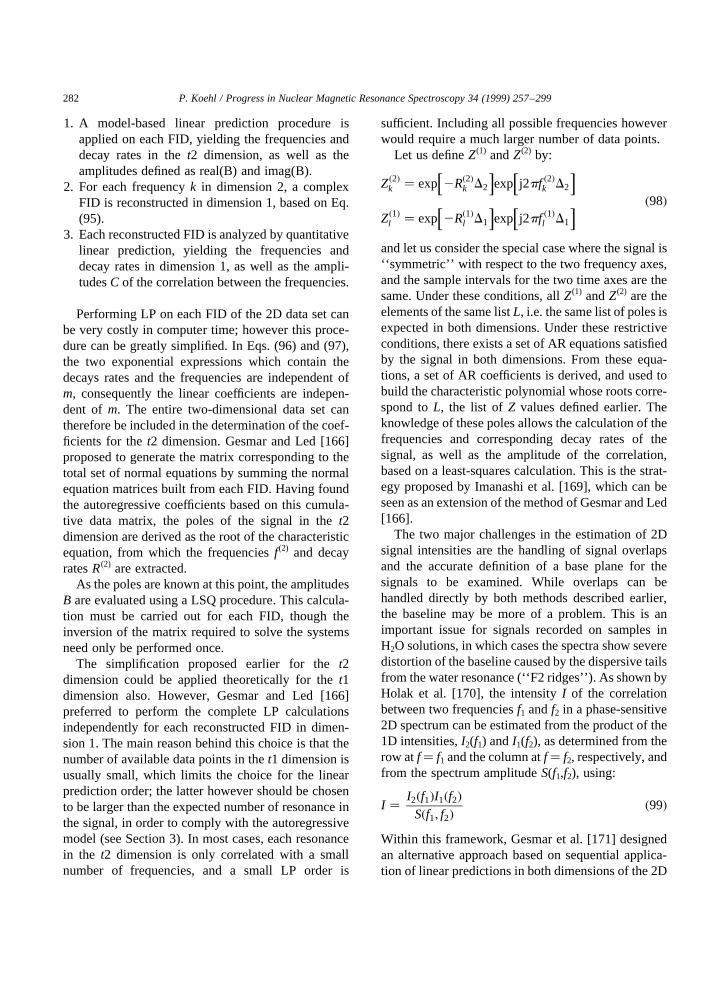
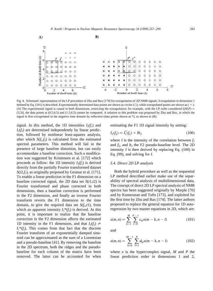
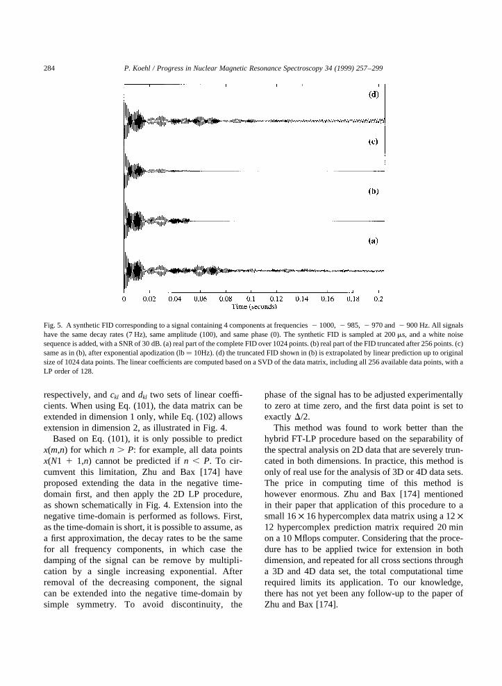
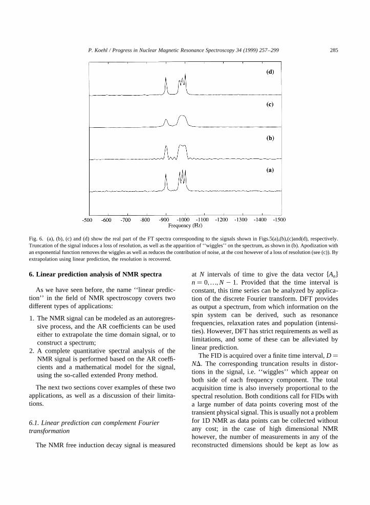
Linear prediction spectral analysis of NMR data P. Koehl a,b a Department of Structural Biology, Fairchild Building, Stanford, CA 94305, USA b UPR 9003 du CNRS, Boulevard Sebastien Brant, 67400 Illkirch-Strasbourg, France Received 10 November 1998 Contents 1. Introduction .................................................................. 258 2. The concept of linear prediction ................................................... 260 2.1. The need for alternative solutions to Fourier transform ............................. 260 2.2. A simple example ........................................................ 261 2.3. Linear prediction: autoregression, or functional modeling? .......................... 261 3. Autoregressive methods ......................................................... 262 3.1. Autoregressive processes ................................................... 262 3.2. Spectrum of an autoregressive time series ...................................... 262 3.3. Computing the autoregressive coefficients: the autocorrelation methods ................. 263 3.4. Noise-free NMR time series are autoregressive processes ........................... 264 3.5. The experimental NMR signal is really an ARMA process .......................... 265 3.6. Computing the autoregressive coefficients: the least squares approach .................. 266 3.6.1. Linear least-squares procedures .......................................... 266 3.6.2. Reducing the contribution of noise ....................................... 268 3.7. Total least-squares approaches ............................................... 272 3.8. Fast linear prediction techniques.............................................. 273 3.9. Conclusions on AR methods ................................................ 274 4. Model-based linear prediction methods .............................................. 274 4.1. The extended Prony method ................................................ 274 4.2. Extracting the frequencies and decay rates ...................................... 276 4.2.1. Roots of the characteristic polynomial ..................................... 276 4.2.2. Avoiding polynomial rooting: The state–space models ......................... 277 4.3. Amplitudes and phases of the signals .......................................... 278 4.4. Conclusions on model-based analysis of NMR signals ............................. 279 5. Linear prediction applied to ND NMR experiments ..................................... 279 5.1. Extracting amplitudes from a ND spectrum ..................................... 279 5.2. Hybrid spectral analysis for ND spectra ........................................ 280 5.3. Spectral analysis using sequential linear prediction. ............................... 281 5.4. Direct 2D LP analysis ..................................................... 283 6. Linear prediction analysis of NMR spectra ............................................ 285 6.1. Linear prediction can complement Fourier transformation ........................... 285 6.2. Complete spectral analysis using linear prediction ................................ 290 6.3. A broader range of application for linear prediction ............................... 292 7. Conclusions .................................................................. 292 Acknowledgements ............................................................... 293 Progress in Nuclear Magnetic Resonance Spectroscopy 34 (1999) 257–299 0079-6565/99/$ - see front matter q 1999 Elsevier Science B.V. All rights reserved. PII: S0079-6565(99)00002-3
Transcript
Linear prediction spectral analysis of NMR data
P. Koehla,b
aDepartment of Structural Biology, Fairchild Building, Stanford, CA 94305, USAbUPR 9003 du CNRS, Boulevard Sebastien Brant, 67400 Illkirch-Strasbourg, France
Keywords:Fourier transformation; Linear prediction; Autoregression methods; Extended Prony method
1. Introduction
Nuclear Magnetic Resonance (NMR) signals wereoriginally derived from continuous wave (CW) spec-troscopy. CW spectra were recorded by slowly andcontinuously scanning the frequency axis, yieldingdirectly all intensities related to the resonancefrequencies contained in the sample of interest [1].The same information however can be obtained byrecording the evolution of a combination of theseintensities with respect to time, after proper prepara-tion, followed by proper deconvolution of the indivi-dual intensities, usually based on Fouriertransformation. The resulting experimental times areconsiderably reduced, and the main advantage is adramatic increase in signal-to-noise ratio. A simpleexplanation for this can be derived from the followingargument. If a combination of two properties P1 andP2 is recorded as a single value, two data points D1and D2 at least are required to retrieve P1 and P2.Assuming that the deconvolution proceeds through alinear combination of the data points D1 and D2, theintensities of the ‘‘signal’’ associated with P1 and P2follow this combination, while error propagationtheory tells us that the ‘‘noise’’ is related only to thesquare root of the combination of errors on D1 and D2(assuming the latter to be independent). Thedevelopment of signal processing techniques, the
introduction of fast techniques to calculate digitalFourier transform such as the Cooley–Tukey algo-rithm [2], as well as the development of the computertechnology transformed this essential finding of Ernstand Anderson [3,4] into a major breakthrough forNMR spectroscopy [5]. Since then, NMR has experi-enced other major changes. An account of these trans-formations can be found in the Nobel lecture of Ernst[6], or in more detail in the recent Encyclopedia ofNMR [7]. Spectrometers with magnets of 14.1 and18.8 T (600 and 800 MHz for1H spectroscopy) arenow quite common for high resolution liquid-stateNMR, and manufacturers have prototypes andprojects for much higher fields. The electronic compo-nents have drastically improved, heading towards afully digital system. A great deal of effort has beenput into developing new experiments [8], which arenow multidimensional [5,9–11], and usually involveseveral spin types [12–15]; the samples themselvesare chemically or biologically modified in order toenrich them in normally rare observable spins, suchas 15N and 13C [16–19], at a reasonable price in thecase of biological samples, as a result of the progressof biotechnologies. All these changes are nowstandard. NMR was at first concerned with interpret-ing spectra in terms of chemical structures, then withspecies identification and dynamics studies. The rangeof applications of NMR techniques has also increased
P. Koehl / Progress in Nuclear Magnetic Resonance Spectroscopy 34 (1999) 257–299258
significantly, including in vivo studies [20–24], aswell as three-dimensional structure determinationand dynamics studies of macromolecules, using highresolution NMR [25–31]. In contrast to all thesechanges, after 30 years, Fourier Transform remainsthe standard procedure for NMR signal processing,though new signal processing techniques haveemerged during the same period of time (for recentreviews, see [32,33]).
It is important to note at this point that signalprocessing in NMR may have very different purposes,depending on the applications. A high resolutionNMR spectroscopist who studies a large biomoleculein solution usually has little a priori knowledgeregarding the spectroscopic properties of the mole-cule. He is first confronted with the problem ofcorrectly identifying in the NMR spectra a largenumber of chemically-shifted nuclei, as well as defin-ing the corresponding underlying chemical structure.The presence of a large number of componentsrequires that sophisticated experimental techniquesbe applied, such as multidimensional spectroscopy.The corresponding experiments are usually costly intime. Signal processing in these cases aims at maxi-mizing the extraction of information from theseexperiments, mainly for the purpose of spectralassignment. In the case of in vivo experiments, thechemical species under study are known, as well astheir NMR spectra. For these applications, signalprocessing is geared toward quantification in thecontext of poor signal-to-noise ratio. Missing datapoints are a common problem in some applicationsof solid state NMR, and signal processing is thenexpected to help recover information from theseincomplete signals. Fourier transformation is themain common denominator in all these forms ofsignal processing. We will see in the following thatit has its limitations.
Fourier analysis provides a mathematical model inwhich any function, and in particular any signal, ismodeled as a sum of sine and cosine waves. Thecoefficients of these waves which provide the bestfit to the original function are stored in the so-calledspectrum, i.e. the Fourier Transform of the signal(see for example [34]). The FT is bijective and hasan inverse (iFT), hence the same information can beretrieved in both the signal (i.e. time-domain infor-mation, referred to as the FID for free induction
decay) and the spectrum (frequency-domain infor-mation). FT operates on continuous functions; anequivalent of FT exists for discrete signals, theDiscrete Fourier Transform, or DFT. Analysis of agiven discrete finite (N values) signal {xn} by meansof DFT assumes only that the signal is sampled withconstant time intervals and that it is zero outside ofthe observation window, which is equivalent tosaying that the signal has been multiplied by theboxcar function (bn � 1 for n � 0,…,N 2 1 and 0otherwise). Solutions have been proposed to allevi-ate the first condition, primarily in the case of a smallnumber of missing data points within a large signal(see for example [35]). Missing data points at thebeginning of the time series are more difficult tohandle, resulting in severe distortions of the baselineof the spectrum. The consequence of the secondcondition (i.e. the multiplication by the boxcar func-tion) is a spectrum distorted by a convolution with aSine Cardinal function (Sinc(x) � sin(x)/x), i.e. theFourier Transform of {bn} shows ‘‘wiggles’’ neareach of its peaks. Attempts to attenuate this problemusually proceed through apodization, of the signal,i.e. multiplication of {xn} by a proper function suchas to set the signal to 0 at the last experimental point.Apodization can either provide improvements inspectral resolution by splitting overlapping peaks,or improvements in the signal-to-noise ratio byrecovering weak signals lost in the noise. Bothenhancements cannot be achieved simultaneously.Also, performance is ultimately limited by theNyquist theorem, which sets the ‘‘dwell time’’, i.e.the sampling time interval, according to the spectralrange of interest. These limits prevent a quantitativeanalysis of crowded spectra which show severe peakoverlaps. In these cases, alternative approaches havebeen proposed, which make use of additional infor-mation, such as models of the underlying physicalsignal and noise in {xn}. These methods includewavelet transforms [36–40], Non-Linear LeastSquares (NLLSQ) fits in the frequency domain[41], Pade–Laplace analysis [42–44], maximumentropy methods [45–52], Bayesian and maximumlikelihood techniques [53–61], genetic algorithms[62], and linear prediction [63–66]. Several reviewsof the latter method have been published (see forexample [41,67–69]). In this review, we will focuson the recent areas of development related to this
P. Koehl / Progress in Nuclear Magnetic Resonance Spectroscopy 34 (1999) 257–299 259
technique, covering both methodological aspectswith emphasis on matrix computation, as well asapplications.
This review is organized as follows. First, theconcept of linear prediction is explained through asimple example. Then, the various numerical techni-ques available for solving the linear prediction equa-tions are described, with emphasis on how they handlenoise in the experimental signal. Qualitative andquantitative issues for linear prediction will becovered in detail. The final section covers all recentapplications of linear prediction in the analysis ofNMR spectra.
The distinction between numerical analysis andengineering has become less well defined in recentyears, and this statement can even be considered aneuphemism in the case of signal processing. In mostpapers dealing with linear prediction, you are likely tosee equations involving matrices covering most of theprinted space. This review is designed to be compre-hensive in describing the new procedures that are nowapplied to linear prediction, therefore will not eludethe technical and mathematical aspects; howeverattempts are made to provide a ‘‘practical’’ explana-tion to the problems as much as possible. I do hopethat after reading this review, the basic conceptsbehind the terms ‘‘linear prediction’’ will be clearer.To help the reader going through the mathematicalformalisms, a small glossary of the main methodsborrowed from applied mathematics is provided atthe end of the manuscript.
2. The concept of linear prediction
2.1. The need for alternative solutions to Fouriertransform
Classical treatment of NMR signals proceedsthrough a discrete Fourier transform (DFT) of thedata points {ak} of a free induction decay (FID),sampled at constant time intervalD:
Ai �XN 2 1
k�0
akexp 2j2pik
N
� ��1�
where j is the complex number whose square is2 1,and N the total number of points. {Ai} is a discreterepresentation of the spectrum of the time domain
signal {ak}, calculated at all frequencies:
fi � iND
; i � 2N2;…;
N2
2 1 �2�
for a complex signal.Despite its popularity, it is important to bear in
mind that the application of DFT imposes certainrestrictions. Firstly, all the elements of the signalmust have been measured at fixed time intervalsD,and included in the calculation. This can be detrimen-tal in certain conditions: should the first data points behighly corrupted by noise, the spectrum will beaccordingly affected, usually showing severe baselineproblems. Ignoring these data points would usuallynot solve this problem, and in fact would inducesevere phase problems. A similar problem exists atthe other end of the time series. Secondly, the derivedspectrum depends onN, the total number of datapoints collected (see Eq. (1)): for example, the digitalresolution in the spectrum is inversely proportional toN. Thirdly, if the data vector is non-zero at the end ofthe acquisition, its Fourier transform exhibits artifacts(i.e. convolution by the Fourier transform of theBoxcar function, defined by B(nD) � 1 for 0 # n ,N and 0 otherwise). While this is usually not aproblem in 1D NMR experiments, in ND experimentsthe number of data points in the reconstructed dimen-sions is usually kept as low as possible in order toreduce the length of the experiment; special care forthe corresponding truncated FID is then needed. Eq.(1) also makes no assumption on the model that bestdescribes the data: this can be seen as an advantage, asit makes DFT universal in its applications, but also asa weakness, as it does not allow inclusion of priorinformation on the signal in the spectral analysis.Eq. (1) is applied to the FID as is, which can beseen as a combination of signal and noise (this combi-nation is usually assumed to be a simple sum), andDFT does not provide a tool to distinguish these twocomponents. All these difficulties have set up thegrounds for the search of alternate spectral analysismethods, Linear Prediction being one of them. Iwould not want to conclude this section by leavingthe impression that Fourier transform should becompletely replaced: though it has its limitations,some of them exposed earlier, DFT is still a veryvaluable technique, routinely used by all NMR spec-troscopists. Interestingly, DFT even proves useful as a
P. Koehl / Progress in Nuclear Magnetic Resonance Spectroscopy 34 (1999) 257–299260
numerical technique to considerably speed up themethods developed to replace it (an example isprovided in the Appendix A).
2.2. A simple example
Let us consider a complex causal signalS(t)containing a single damped exponential:
S�t� � Ae2Rte2j2pf0t �3�whereA is a complex amplitude,R the damping coef-ficient, andf0 the frequency of the sinusoid.
SamplingS(t) at constant time intervalD yields thetime series {Sk}:
Sk � S�kD� � Ae2RkDe2j2pf0kD � AZk �4�whereZ is a constant with respect tok, and equal to:
Z � e2�R1j2pf0�D �5�Using basic properties of exponential functions, wedirectly derive from Eq. (4) that:
Sk � ZSk21 ;;k . 0 �6�i.e. the data points in the time series are linearlyrelated. In this simple case, knowledge of two conse-cutive data pointsSi andSi11 is enough to fully char-acterize the time series, by first computingZ� Si11/Si.This has several major consequences.
1. All data points precedingSi or following Si11 canbe derived by successive applications of Eq. (6).This is the concept of backward and forward linearprediction, respectively.
2. If N data points have been collected, the procedureaforementioned would make it possible to build aprolonged signal with much more data points thanN. This would be useful ifN is small and the timeseries is meant to be analyzed by Fourier trans-form, in which case artifacts related to truncationcould be removed.
3. In fact, there is no need to prolong the time seriesSas its spectrum can be directly derived based solelyon Eq. (6).The Fourier transformX(f) of the timeseriesS is defined by:
X�f � �X1 ∞
k�0
Skexp 2j2pfkD� � �7�
By summing Eq. (6) multiplied by exp2j2pfkD� �
for all k . 0, we get:X1 ∞
k�1
Skexp 2j2pfkD� � � Z
X1 ∞
k�1
Sk21exp 2j2pfkD� �
:
�8�Substituting Eq. (5) in Eq. (6), we obtain, afterrearrangement:
X�f �2 S0 � Z exp 2j2pfD� �
X�f �: �9�Thus the Fourier transform ofS is:
X�f � � A1 2 Z exp 2j2pfD
� � �10�
4. If finally we use the fact that the time seriesS is adiscrete representation of the model function givenby Eq. (3), the spectrum itself becomes useless: thedamping coefficientR and the frequencyf0 can bedirectly derived from the module and phase ofZ:
R� 21D
lnuZu �11�
and
f0 � 21
2pDarg�Z� �2p� �12�
and the amplitudeA is subsequently derived fromEq. (4), yielding all elements of the signal (theambiguity in the definition of the frequency is aconsequence of the discretization of the signal;the equivalent in the Fourier analysis is the peri-odicity of the continuous or discrete spectrum).
2.3. Linear prediction: autoregression, or functionalmodeling?
The relevant point to be deduced from the simpleexample described earlier is that if the time seriesunder study satisfies a relationship similar to Eq. (6),then, even if it is short, it may contain enough infor-mation to allow a correct spectral analysis. Theproblem is to recover this information. When theonly knowledge we rely on is Eq. (6), this leads tothe concept of autoregressive modeling (AR) [70]. Ifin addition the underlying model for the time series isknown (such as Eq.(3) for the example given earlier),then the problem becomes deterministic, in which
P. Koehl / Progress in Nuclear Magnetic Resonance Spectroscopy 34 (1999) 257–299 261
case more restrictive but more robust techniques forextracting information on the signal exist; these tech-niques belong to functional modeling. Linear predic-tion is in fact a generic term which describes bothapproaches [67,70].
Autoregressive time series have properties whichgreatly facilitate their analyses; in particular, theycan be extrapolated in the ‘‘future’’ or in the ‘‘past’’(i.e. after the last data point, or before the first datapoint, respectively). Such properties are potentiallyvery useful for the analysis of NMR signals. In thecase of high-dimensional NMR for example,experimental time considerations limit the numberof acquired data points in the reconstructed dimen-sions; direct application of Fourier transform on thisdata induces distortions, which can be reduced byapodization prior to DFT, but at the cost of loss ofresolution.
In the following section, we will briefly defineautoregressive processes, as well as the commonmethods to study them. We will then show thatunder certain assumptions, an NMR signal satisfiesthe requirements of AR processes, but its analysisrequires specific techniques, which will be reviewedin detail.
Functional modeling is described in detail inSection 4.
3. Autoregressive methods
3.1. Autoregressive processes
Let us consider a discrete time series as a noisyrepresentation of a deterministic phenomenon. Thetotal acquisition lastsND, whereN is the number ofdata points andD the constant time interval betweentwo points. Assuming that this window of observationprovides a quasi-complete image of this phenomenon,it is quite natural to express any data pointam notmeasured as a function ofM known experimentalpoints:
am � f aN21;…;aN2M
ÿ �for m . N 2 1 �13�
whereM is a parameter at this stage.The simplest possible expression for the function
f(aN21,…,aN2M) is linear; we could then predictaN
based on the relationship:
aN �XMm�1
bmaN2m 1 eN �14�
whereM is the order of the linear estimator, theb arecoefficients, andeN is noise. More generally, we willassume:
ak �XMm�1
bmak2m 1 ek �15�
for all k (i.e. Eq. (15) applies on known datapoints as well as outside of the observationwindow); ek is the k-th element of a zero-mean, white noise vector. Time series thatcomply with Eq. (15) are referred to as auto-regressive processes [70]; sinusoids are goodexamples of underlying models for these types oftime series.
3.2. Spectrum of an autoregressive time series
One of the major interests of AR analysis is that itallows direct calculation of the spectrum of the timeseries, bypassing the Fourier analysis. Following themethod used in the simple example described earlier,we multiply Eq. (15) by exp2j2pfkD
� �and sum over
all k:
X1 ∞
k�2 ∞akexp 2j2pfkD
� �
�X1 ∞
k�2 ∞
XMm�1
bmak2mexp 2j2pfkD� �
1X1 ∞
k�2 ∞ekexp 2j2pfkD
� � �16�
(the summation extends to allk, positive and negative,as this approach is not restricted to causal time series).By definition, the left side of Eq. (16) corresponds toA(f), the Fourier transform of the time series {ak},while the last term of the right term isE(f), theFourier transform of the noise sequence {ek}. After
P. Koehl / Progress in Nuclear Magnetic Resonance Spectroscopy 34 (1999) 257–299262
rearrangement, we obtain:
A�f � �XMm�1
bmexp 2j2pfmD� � X1 ∞
k�2 ∞ak2m
exp 2j2pf �k 2 m�D� �1 E�f �
�17�
Eq. (17) can be rewritten as:
A�f � �XMm�1
bmexp 2j2pfmD� �
A�f �1 E�f � �18�
which yields, after settingb0 � 2 1,
A�f � � 2E�f �PM
m�0bmexp�2j2pfmD�
�19�
As {ek} is supposed to be a white noise with zeromean, its Fourier transformE(f) is a constant, inwhich case the Fourier transform of the time signalis directly derived from the knowledge of the predic-tion coefficients {bm}.
A word of caution is in order here: Eq. (19) woulddirectly provide the spectrum of the signal understudy, were it not from the fact that the summationof the Fourier series in Eq. (16) extends from2 ∞ to1 ∞. Experimental signals are causal however, andfinite in size. While this is not a problem when apower spectrum is sufficient, deriving phased spectrarequires more precaution. Solutions to this problemhave been described by Tang and Norris [71–73] inthe form of the LPZ transform, and by Ni andScheraga [74].
3.3. Computing the autoregressive coefficients: theautocorrelation methods
It is important to notice that in the AR masterequationek is completely included in the model:Eq. (15) cannot be considered as the summation ofsignal and noise, asek depends on the previoussequence {e0,…,eN21}. A crude but reasonablestatement would be that in AR, the existence of obser-vation noise is neglected, and the white ‘‘noise’’sequenceek is a measure of the validity of the predic-tion model.
The method used to solve for the coefficientsbm
is called regression analysis or alternatively auto-regressive (AR) model, as the summation extends
over the ‘‘past’’ of the time series. Two differentapproaches for solving for thebm have beenproposed [67]: the first is based on the auto-correlation coefficients of the data points, whilethe second directly analyzes the data pointsthemselves.
If we assume that the time series to be analyzed isstationary with zero mean, estimates of the autocorre-lation coefficients are given by:
Rn � 1N 2 n
XN 2 n2 1
k�1
ak1na*k �20�
where * stands for the complex conjugate.Rn can also be seen as an estimate of the true
autocorrelation coefficientsRn, which are equal tothe expectation valueE ak1na*k
� �, or equivalently
E aka*k2n
� �. The latter can be obtained by
multiplying Eq. (15) by a*k2n, and taking theexpectation:
E aka*k2n
� � � E 2XMm�1
bmak2ma*k2n
" #1 E eka*k2n
� ��21�
As the data pointsak2n are uncorrelated with thewhite ‘‘noise’’ ek for n . 0, we obtain:
Rn � 2XMm�1
bmRn2m �22�
and, for n � 0,
R0 � 2XMm�1
bmR2m 1 s2 �23�
where R2m � R*m and s2 � E�eke*k�, i.e. thevariance of the white ‘‘noise’’ sequence {ek}.Combining Eq. (22) and Eq. (23), and settingb0 � 1, we obtain [70]:
XMm�0
bmRn2m �s2 n� 0
0 n . 0:
(�24�
Eq. (24) corresponds to the Yule–Walker equa-tions, which show that the linear coefficientsbm
can be derived from the autocorrelation coeffi-cients.
The Yule–Walker equations can be rewritten in
P. Koehl / Progress in Nuclear Magnetic Resonance Spectroscopy 34 (1999) 257–299 263
matrix form as:
R0 R21 : : : R2M
R1 R0 : : : R12M
: : : :
: : : :
: : : :
RM RM21 : : : R0
26666666666664
37777777777775
1
b1
:
:
:
bM
26666666666664
37777777777775�
s2
0
:
:
:
0
266666666666664
377777777777775�25�
where the matrixR on the left hand side is called theautocorrelation matrix, which has an hermitianToeplitz structure (see Glossary). The unknowns inthe system of Eq. (25) are the linear coefficients {b}and s 2 which can be retrieved either by classicalmatrix operations, or by using the fast Levinson andDurbin algorithm [75,76]. The latter takes in accountthe Toeplitz structure of the matrix.
The major assumption when solving the Yule–Walker equations is that the true autocorrelation coef-ficientsRn can be safely replaced by the estimatesRn
given by Eq. (20). While for largeN and smalln thiscan be seen as reasonable (i.e. the sum will containenough terms to average out the experimental noise),Rn will be a poor estimate for largen and more gener-ally for small N, as well as for signals with poorsignal-to-noise ratio and for non stationary signals.Several methods have been proposed to try to alleviatethese problems.
1. Burg proposed a modification of the Levinson–Durbin algorithm with built-in construction of theestimates of the autocorrelation coefficients[77,78]. This method works directly on the datamatrix, and makes no assumptions about elementsoutside the observation range, from 0 toN 2 1 (thismethod is sometimes referred to as a maximumentropy technique, though it is a true LP techni-que). Though this method is an improvementcompared to solving directly the Yule–Walkerequations, problems have been reported, such asline splitting (appearance of two lines where oneis expected) [79], and frequency shifting [80,81].
2. For transient time series, Cadzow proposed tomodify the number of terms included in theestimation ofRn based on its row position in the
correlation matrix [82]; this has the drawback ofdestroying the Toeplitz structure of this matrix,making the procedure inefficient.
3. Fedrigo et al. [83] proposed a modification of Eq.(20) in which the number of terms included in thesummation becomes independent ofn:
Rn � 1K
XK 2 1
k�0
ak1na*k �26�
When this modification is used, the Toeplitz struc-ture of the matrix is maintained. This method,which is based on a modified correlation matrix,was shown on a few examples to perform betterthan a method working directly on the raw data,though it is not clear from their paper whichmethod was used for the latter.
3.4. Noise-free NMR time series are autoregressiveprocesses
The NMR signal is a transient process recorded as afinite time series {An} which can be modeled by afunction An, consisting ofK exponentially dampedsinusoids characterized by signal frequenciesfk,
amplitudes ck, damping factorsRk and phasew k,defined by:
An �XKk�1
ckejwke�2Rk1j2pfk�nD �27�
whereD is the constant sampling time interval. As afirst step, noise is not considered. Any signal whichcan be described by Eq. (27) verifies the AR equationexactly, with an order parameterM� K. This propertywas introduced two centuries ago by the Baron deProny [63], and was recently re-introduced in signalprocessing of NMR data by Kay and Marple [84]. Abrief description of why Eq. (27) verifies the AR equa-tions, and how it can be used to analyze NMR signalfollows. Let us define:
Zk � e�2Rk2i2pfk�D �28�and P the complex polynomial function of orderK,whoseK roots are theZk:
P�z� �YKk�1
�z2 zk� �29�
P. Koehl / Progress in Nuclear Magnetic Resonance Spectroscopy 34 (1999) 257–299264
After expansion,P can be rewritten as:
P�z� � zK 2XKm�1
bmzK2m �30�
wherebm are coefficients.As by definition ofP, P(Zk)� 0 for all k, the follow-
ing relation:
ZKk �
XKm�1
bmZK2mk �31�
are true for allk in[1,K]. More generally,
Znk �
XKm�1
bmZn2mk ; n $ K �32�
Combining Eqs. (27), (28) and (32), we obtain:
An �XKk�1
ckejwk
XKm�1
bmZn2mk
!�33�
from which we derive:
An �XKm�1
bmAn2m �34�
for all n larger thanK.Eqs. (27)–(34) provide a justification for the fact
that an NMR signal follows an AR model [Eq. (34)should be directly compared to Eq. (15)]. The maindifference lies in the fact that there is no need toinclude the white noise sequenceen, as the linear rela-tion (34) is exact. It should be emphasized again atthis point that {en} in the AR model is a measure ofthe validity of the model, and does not account formeasurement noise; the latter has not yet beenincluded here. It is also interesting to notice that thepolynomial introduced in Eq. (30) corresponds in factto the denominator of the spectrum of the time series,as determined using the AR model (Eq. (19)). Thoughthe {Zk} values are truly roots of the polynomialP,they can be seen as ‘‘poles’’ of the spectrum of thetime series. For this reason, they are usually referredto as poles, andK, the number of sinusoids to bemodeled, is sometimes referred to as the number ofpoles included in the calculation.
The theoretical time series described by Eq. (27)can be prolonged by an arbitrary number of points
using Eq. (34): performing this extrapolation isdefined as ‘‘forward linear prediction’’.
The same reasoning which prevails for Eqs. (28)–(34) can be repeated to define backward linear predic-tion, in which case:
An �XKm�1
cmAn1m �35�
In Eq. (35), {c} are the backward linear predictions.
3.5. The experimental NMR signal is really an ARMAprocess
Under the assumption that the true NMR signals areexponentially damped sinusoids, i.e. that (26)describes the NMR free induction decay (FID) inthe absence of noise, the data points of an experimen-tal FID in the presence of noise can be modeled by
An � A�nD� � An 1 wn;n� 0; 1……N2 1 �36�whereN is the total number of data points. The noisesequencewn is supposed to be normally distributed,with zero mean and a standard deviations , and thereal and imaginary part ofwn are supposed to be inde-pendent. After substitution of Eq. (36) into Eq. (34),we obtain:
An 2 wn �XKk�1
bk�An2k 2 wn2k� �37�
hence:
An �XKk�1
bkAn2k 2XKk�1
bkwn2k 1 wn �38�
A true least-squares solution vector {b} of Eq. (38)would minimize the variance ofw defined asXNk�1
w*kwk �39�
This would lead however to a set of nonlinear equa-tions.
Based on Eq. (38),An is in fact an autoregressive-moving average process (ARMA), with identicalautoregression and moving average parameters [70].The estimation of ARMA parameters is complex, andremains an active area of research [85–93]. A widelyused procedure is to exploit the fact that an ARMA
P. Koehl / Progress in Nuclear Magnetic Resonance Spectroscopy 34 (1999) 257–299 265
process can be expressed as an AR process of infiniteorder [70]. Eq. (38) is then rewritten as:
An �XPk�1
bkAn2k 1 1n �40�
in which the noise is now modeled byen. The order ofthe sum has been modified fromK, the true number ofunderlying sinusoids, toP, a parameter referred to asthe order of the LP procedure, withP . K. It shouldbe mentioned thatK is usually not known, in whichcase increasing the LP order toP has the furtheradvantage of ensuring the determination of allcomplex exponentials in the signal.
As a first approximation, it is therefore appropriateto analyze an NMR signal as an AR process. The firststep of such a study is to find the coefficients of thelinear relations between the data points. Under theergodic condition these coefficients can be derivedfrom the autocorrelation matrixR, using the Yule–Walker equations [see Eq. (25)]. Fast algorithms areusually applied to this problem such as the Levinson–Durbin procedure, which uses the special Toeplitzstructure of the matrixR. NMR signals however arenot stationary, and discarding this fact leads to poorresults when applying AR (for a review see [41,67]).Solutions to this problem have been proposed, such asthe Burg algorithm described earlier, which is directlyapplied on the data matrix [77,78]. It was shownhowever that even this procedure has problems, suchas a line splitting when a single line is expected [79]and frequency shifting [80,81]. The most promisingalternative techniques are least-squares methods,which make no assumptions on data points outsidethe window of observation, as well as on the ergodi-city of the signal.
3.6. Computing the autoregressive coefficients: theleast squares approach
3.6.1. Linear least-squares proceduresLet us consider a classical linear system of equa-
tion:
Ax � b 1 n �41�wheren is a noise sequence affecting the observationvectorb, supposed to be white and of zero mean. Aleast-squares solution of Eq. (41) is obtained byminimizing the variance ofn, or equivalently the
difference squared between the modelAx and theobservation vectorb:
xLSQ � arg minx�n*n� � arg min
xiAx 2 bi2� �
�42�
wheren* is the hermitian transpose ofn, andi·i theL2 norm [94].
This procedure can be directly applied to Eq. (40):under the assumption thate is a white noise process,with zero mean, a minimum variance estimate ofb,bLSQ, is obtained by minimizinge*e , based on Eq.(42). Several methods have been proposed to solvethis problem, and we will review some of them. Letus first rewrite Eq. (40) in matrix form as:
AP21 AP22 : : A0
AP AP21 : : A1
: : : : :
: : : : :
AN22 AN23 : : AN21 2P
26666666664
37777777775
b1
b2
:
:
bP
26666666664
37777777775
�
AP
AP11
:
:
AN21
26666666664
377777777751
1P
1P11
:
:
1N21
26666666664
37777777775�43�
whereN is the total number of data points in the NMRsignal, andP the number of poles; we have seenearlier thatP should be as large as possible. FromEq. (41) however, we also observe that the largestpossible value forP is N/2.
Notice that in Eq. (43), the prediction remains onthe available data, i.e. for example Eq.(40) is notapplied forn , P. This is different from the autore-gressive methods based on the correlation matrixdescribed, which use all possible equations, fillingup with zeros when data points are ‘‘missing’’. Ifthe larger system which includes these incompleteequations had be considered instead, its normalequations would have led back to the Yule–Walkerequations, with all the problems mentioned earlier.The reduced system of equations described by Eq.(43) is known as the covariance method of linearprediction.
P. Koehl / Progress in Nuclear Magnetic Resonance Spectroscopy 34 (1999) 257–299266
Eq. (43) can be restated in compact form
Tb � a 1 1 �44�whereT and a are a matrix and a vector containingsignal data points, respectively.
T is highly structured, in the sense that all elementson any sub-diagonal ofT are equal:T is a Toeplitzmatrix (see Glossary). It should be noted that bysimple manipulation, Eq. (43) can be rewritten as:
A0 A1 : : AP21
A1 A2 : : AP
: : : : :
: : : : :
AN212P AN2P : : AN22
26666666664
37777777775
bP
b1
:
:
b1
26666666664
37777777775
�
AP
AP11
:
:
AN21
26666666664
377777777751
1P
1P11
:
:
1N21
26666666664
37777777775�45�
or in compact form as:
Hb � a 1 1 �46�whereH is a matrix in which all elements in a given
anti-diagonal are equal:H is a Hankel matrix. Bothforms of the system have been used in NMR. AsToeplitz and Hankel matrices have very similar prop-erties, we will focus only on the Toeplitz representa-tion.
The dimension ofT is (N 2 P) × P, hence the directinverse ofT cannot be computed. The most commonapproach is to form the normal equations [94]:
T*Tb < T*a �47�where < indicates that the noise is not considered. Inthe specific case of linear prediction in which thematrix T is Toeplitz, building the normal equationsis fast. Thus, let us callC � T*T, then
C�i; j� �XN 2 P
k�1
E�k; i�*E�k; j� for �i; j� [ �1;P�2 �48�
where
E�k; i� � AP111i2j �49�from the definition of the signal matrix.C is hermi-tian; in addition, if we considerC(i 1 1,j 1 1), weobtain:
C�i 1 1; j 1 1� �XN 2 P
k�1
AP111k2i21*AP111k2j21
�XN 2 P2 1
k�0
AP111k2i *AP111k2j �50�
hence
C�i 1 1; j 1 1� � C�i; j�1 AP112j *AP112i
2 AP111N2j *AP111N2i �51�The whole correlation matrixC can then be
constructed at low computing cost from the knowl-edge of its first column and successive use of Eq. (51).In addition, the first column ofC is obtained as theproduct of the Toeplitz matrixT* with the vectorcorresponding to the first column ofT, and thecomputational cost for that product can be reducedfrom N2 in general to N log(N), using FFT (seeAppendix A). The only drawback of this procedureis thatC � T*T does not have a particular structureanymore.
The least squares solution of (42) is derived as:
bLSQ � �T*T�21T*a �52�Eq. (50) can be simplified by first taking the Choleskydecomposition ofT:
T*T � S*S �53�whereS is an upper triangular matrix. This method isusually preferred to a LU decomposition of the samematrix, as it is faster and allows direct identification ofthe pseudo-rank of the system. It has been applied toLP in NMR by Gesmar and Led [95].
Even though the normal equations can be formedfast, other numerically more stable approaches havebeen proposed, either based on a Householder QRdecomposition ofT(T � QR, whereR is upper trian-gular, andQ orthogonal), or by first calculating thepseudo-inverse ofT, using its singular value decom-position (SVD). The two latter approaches are
P. Koehl / Progress in Nuclear Magnetic Resonance Spectroscopy 34 (1999) 257–299 267
referred to as LPQRD [96] and LPSVD [66], respec-tively, for obvious reasons.
3.6.2. Reducing the contribution of noiseThere is no physical reason fore in Eq. (40) to be a
white noise vector with zero mean. In fact, we knowthat:
1n � 2XPk�1
bkwn2k 1 wn �54�
hence LSQ estimates ofb based on Eq. (40) can bebiased. A further complication occurs asK, the truenumber of sinusoids, is usually unknown. A first
approximation to minimize both problems is toincrease the number of forward prediction coefficientsto P larger thanK, with the hope that this will alsoincrease the resolution in the frequency domain.Increasing the number of prediction coefficients hasbeen shown to be useful without complete success inremoving the bias (see for example [95,97]). Problemsoccur in the analysis of short NMR time series, inwhich case the value ofP is limited, and in theanalysis of FIDs with poor signal-to-noise ratios. Inthe latter case, there is the cumulative effect of theincrease of observation noise, and the increase in thelimitation of the model, which tries to fit an ARmodel to the noise in the signal. This can affect the
P. Koehl / Progress in Nuclear Magnetic Resonance Spectroscopy 34 (1999) 257–299268
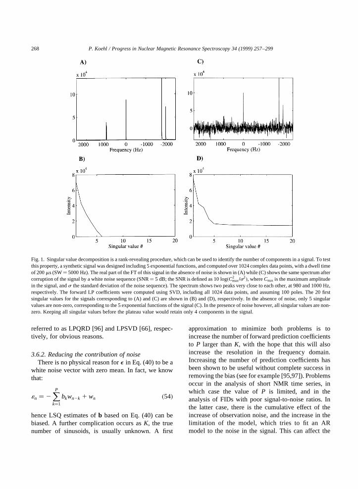
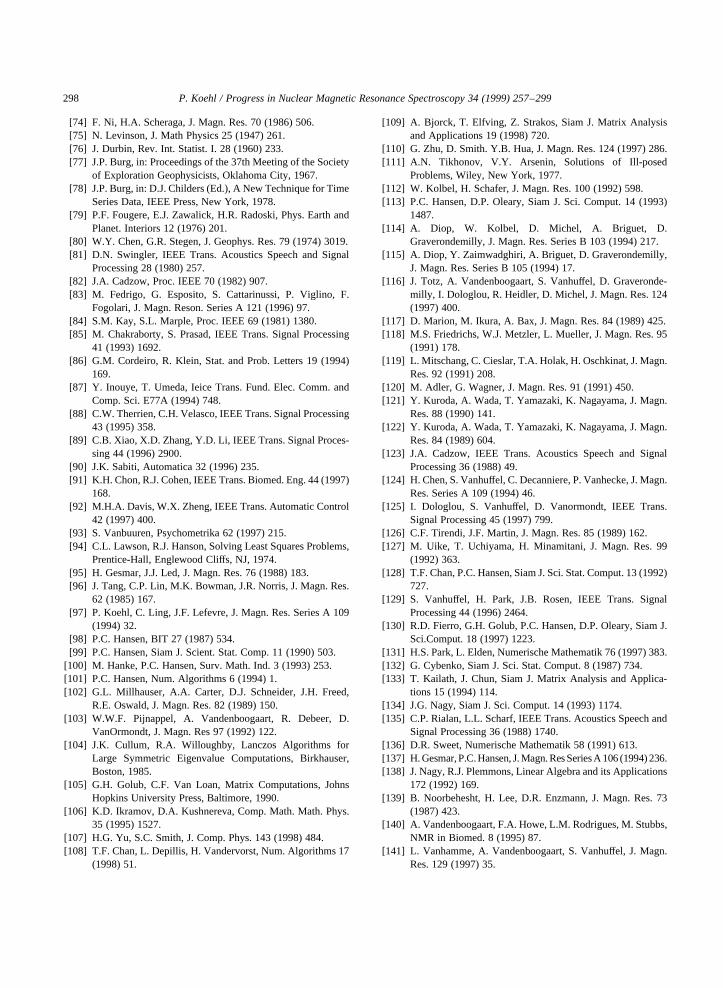
Fig. 1. Singular value decomposition is a rank-revealing procedure, which can be used to identify the number of components in a signal. To testthis property, a synthetic signal was designed including 5 exponential functions, and computed over 1024 complex data points, with a dwell timeof 200ms (SW� 5000 Hz). The real part of the FT of this signal in the absence of noise is shown in (A) while (C) shows the same spectrum aftercorruption of the signal by a white noise sequence (SNR� 5 dB; the SNR is defined as 10 log�C2
max=s2�, whereCmax is the maximum amplitude
in the signal, ands the standard deviation of the noise sequence). The spectrum shows two peaks very close to each other, at 980 and 1000 Hz,respectively. The forward LP coefficients were computed using SVD, including all 1024 data points, and assuming 100 poles. The 20 firstsingular values for the signals corresponding to (A) and (C) are shown in (B) and (D), respectively. In the absence of noise, only 5 singularvalues are non-zero, corresponding to the 5 exponential functions of the signal (C). In the presence of noise however, all singular values are non-zero. Keeping all singular values before the plateau value would retain only 4 components in the signal.
computation of the linear prediction coefficients intwo ways: firstly, the data matrix can become numeri-cally unstable, resulting in poor solutions for thelinear system to be solved, and secondly the ARmodel itself might not apply anymore. Solutions tothese problems would involve modification of thematrix itself to prevent numerical problems, andpre-treatment of the data in the signal themselves, inorder to reduce the contribution of noise. This has ledto the application for LP of two numerical procedures,namely regularization and preprocessing, which arepresented in detail in the following.
3.6.2.1. Regularization We will briefly describe theconcept of regularization in the case of SVD-basedleast-squares methods [98,99]. A general overviewof regularization can be found in [100,101]; anillustration is provided in Fig. 1.
Let us go back to the problem of solving Eq. (46),which can be restated in terms of ax 2:
bLSQ � minb
x2 � minb
iTb 2 ai2� �
�55�
As we have seen before, several methods exist tosolve the corresponding system; we will focus hereon the SVD approach. The singular value decomposi-tion of the data matrixT of size (N 2 P)*P is definedas:
T � UStV �56�whereU andV are orthogonal matrices containing thesingular vectors, andS the diagonal matrix containingthe singular values. In the absence of noise, the rank ofT is exactlyK, the total number of exponentials in thesignal, and onlyK singular values are non-zero (anexample is given in Fig. 1(b)). The least-squares solu-tion of Eq. (56) is then defined as:
bLSQ � VS0tUa �57�whereS0 is the pseudo-inverse ofS:
S�i; i� �1
S�i; i� ; S�i; i� ± 0
0; S�i; i� � 0
:
8><>: �58�
In the presence of noise however, all singularvalues are usually greater than zero (Fig. 1(d)). Directapplication of Eq. (58) can lead to a distorted solution:a small value ofS(i,i), which could probably be
accounted for by noise, will yield an unrealisticlarge pseudo-inverse element, resulting in a leastsquares solution which is too large. This is used infact to characterize the ‘‘instability’’ or ill-condition-ing of the matrix, by defining its condition number as(see also the Glossary):
cond�T� � S�1; 1�S�P;P� �59�
i.e. the ratio of the largest to the smallest singularvalue. The condition number is always larger than 1,and becomes infinite when the matrix is rank defi-cient. A small value for cond(T) indicates thatT isfull rank, and numerically stable, while large valuesfor cond(T) indicates instability. In the latter case infact, the matrix is probably not full rank, and it is onlyfor numerical reasons that it appears as such.
If the true rankK of T is known in advance, asimple solution is to setS(i,i) � 0 for all i largerthanK. This procedure is referred to as discrete regu-larization, and has been applied in the case of LPSVDto NMR signals [65]. It is worth noticing that whenKis known, the regularization scheme described here issuch that only the firstK singular values ofT areneeded. If only a small number of singular valuesare to be computed, alternative schemes to classicalSVD exist, such as the Lanczos algorithm which hasbeen used for analyzing NMR signals [102,103]. Thebasic Lanczos algorithm [104,105] is known howeverto be very sensitive to round-off errors [103], and anumerically stable implementation requires greatcare. The method is still the subject of much research[106–109].
Small singular values correspond to noise. Inver-sely, the largest singular value usually corresponds tothe predominant component in the signal, i.e. usuallythe solvent. This has led Zhu et al. [110] to propose apost-acquisition solvent processing technique, inwhich they first build the data matrix, calculate itsSVD, set the first singular value to zero, and thenreconstruct a signal which is analyzed by FT. It shouldbe mentioned that such an application may lead todistortion in the amplitudes of the signal, as there isno reason to expect that the first singular value willrefer to the water resonance only.
If the noise level is low andK is not known inadvance, it can in principle be estimated from thespectrum of the singular values, as the singular values
P. Koehl / Progress in Nuclear Magnetic Resonance Spectroscopy 34 (1999) 257–299 269
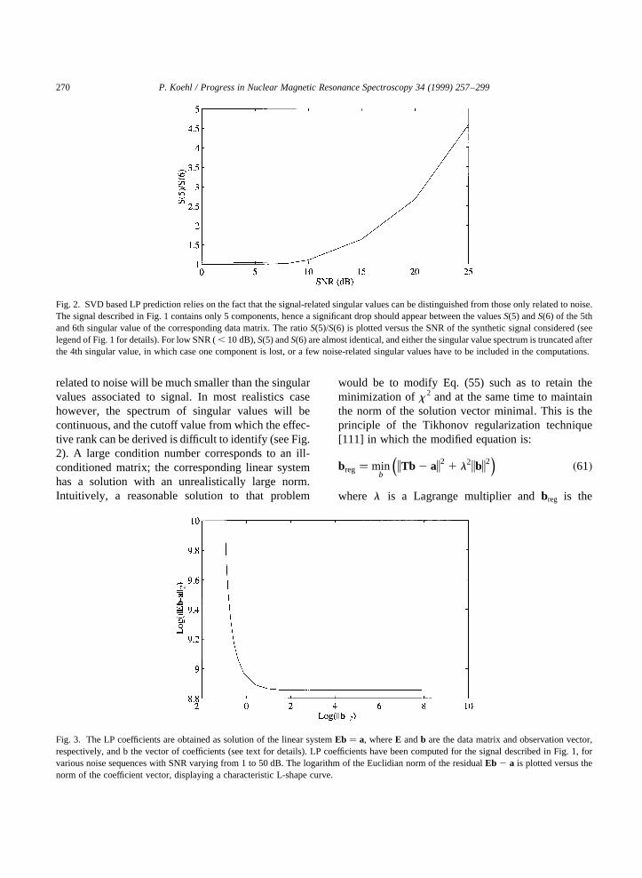
related to noise will be much smaller than the singularvalues associated to signal. In most realistics casehowever, the spectrum of singular values will becontinuous, and the cutoff value from which the effec-tive rank can be derived is difficult to identify (see Fig.2). A large condition number corresponds to an ill-conditioned matrix; the corresponding linear systemhas a solution with an unrealistically large norm.Intuitively, a reasonable solution to that problem
would be to modify Eq. (55) such as to retain theminimization ofx 2 and at the same time to maintainthe norm of the solution vector minimal. This is theprinciple of the Tikhonov regularization technique[111] in which the modified equation is:
breg� minb
iTb 2 ai21 l2ibi2
� ��61�
where l is a Lagrange multiplier andbreg is the
P. Koehl / Progress in Nuclear Magnetic Resonance Spectroscopy 34 (1999) 257–299270
Fig. 2. SVD based LP prediction relies on the fact that the signal-related singular values can be distinguished from those only related to noise.The signal described in Fig. 1 contains only 5 components, hence a significant drop should appear between the valuesS(5) andS(6) of the 5thand 6th singular value of the corresponding data matrix. The ratioS(5)/S(6) is plotted versus the SNR of the synthetic signal considered (seelegend of Fig. 1 for details). For low SNR (, 10 dB),S(5) andS(6) are almost identical, and either the singular value spectrum is truncated afterthe 4th singular value, in which case one component is lost, or a few noise-related singular values have to be included in the computations.
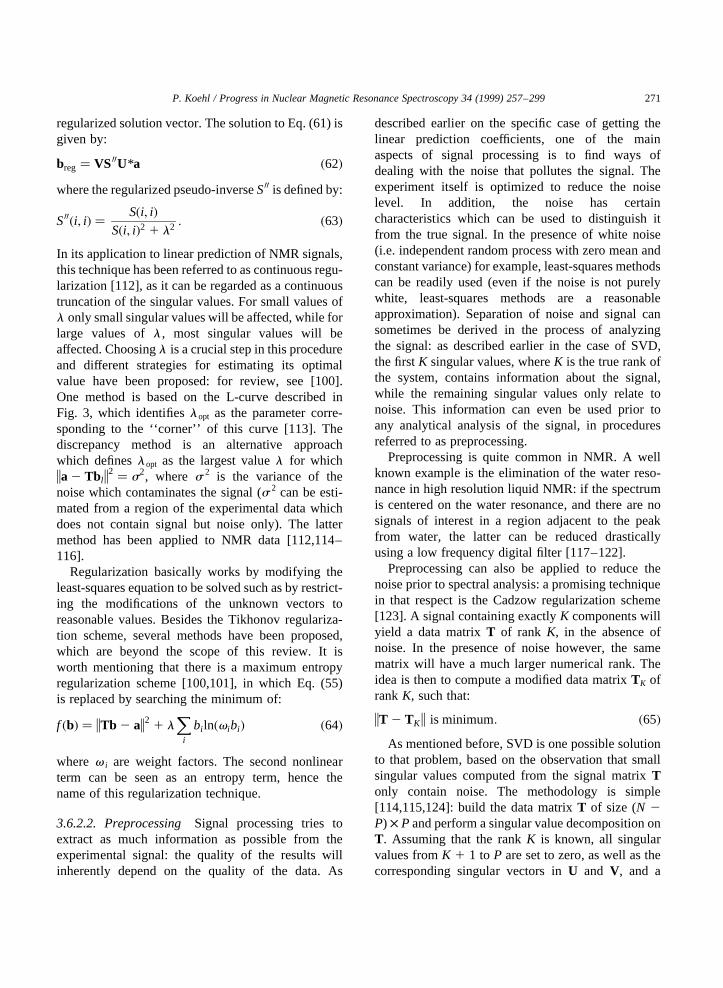
Fig. 3. The LP coefficients are obtained as solution of the linear systemEb � a, whereE andb are the data matrix and observation vector,respectively, and b the vector of coefficients (see text for details). LP coefficients have been computed for the signal described in Fig. 1, forvarious noise sequences with SNR varying from 1 to 50 dB. The logarithm of the Euclidian norm of the residualEb 2 a is plotted versus thenorm of the coefficient vector, displaying a characteristic L-shape curve.
regularized solution vector. The solution to Eq. (61) isgiven by:
breg� VS00U*a �62�where the regularized pseudo-inverseS00 is defined by:
S00�i; i� � S�i; i�S�i; i�2 1 l2 : �63�
In its application to linear prediction of NMR signals,this technique has been referred to as continuous regu-larization [112], as it can be regarded as a continuoustruncation of the singular values. For small values ofl only small singular values will be affected, while forlarge values ofl , most singular values will beaffected. Choosingl is a crucial step in this procedureand different strategies for estimating its optimalvalue have been proposed: for review, see [100].One method is based on the L-curve described inFig. 3, which identifieslopt as the parameter corre-sponding to the ‘‘corner’’ of this curve [113]. Thediscrepancy method is an alternative approachwhich defineslopt as the largest valuel for whichia 2 Tb li
2 � s2, where s 2 is the variance of thenoise which contaminates the signal (s 2 can be esti-mated from a region of the experimental data whichdoes not contain signal but noise only). The lattermethod has been applied to NMR data [112,114–116].
Regularization basically works by modifying theleast-squares equation to be solved such as by restrict-ing the modifications of the unknown vectors toreasonable values. Besides the Tikhonov regulariza-tion scheme, several methods have been proposed,which are beyond the scope of this review. It isworth mentioning that there is a maximum entropyregularization scheme [100,101], in which Eq. (55)is replaced by searching the minimum of:
f �b� � iTb 2 ai21 l
Xi
bi ln�vibi� �64�
wherev i are weight factors. The second nonlinearterm can be seen as an entropy term, hence thename of this regularization technique.
3.6.2.2. PreprocessingSignal processing tries toextract as much information as possible from theexperimental signal: the quality of the results willinherently depend on the quality of the data. As
described earlier on the specific case of getting thelinear prediction coefficients, one of the mainaspects of signal processing is to find ways ofdealing with the noise that pollutes the signal. Theexperiment itself is optimized to reduce the noiselevel. In addition, the noise has certaincharacteristics which can be used to distinguish itfrom the true signal. In the presence of white noise(i.e. independent random process with zero mean andconstant variance) for example, least-squares methodscan be readily used (even if the noise is not purelywhite, least-squares methods are a reasonableapproximation). Separation of noise and signal cansometimes be derived in the process of analyzingthe signal: as described earlier in the case of SVD,the firstK singular values, whereK is the true rank ofthe system, contains information about the signal,while the remaining singular values only relate tonoise. This information can even be used prior toany analytical analysis of the signal, in proceduresreferred to as preprocessing.
Preprocessing is quite common in NMR. A wellknown example is the elimination of the water reso-nance in high resolution liquid NMR: if the spectrumis centered on the water resonance, and there are nosignals of interest in a region adjacent to the peakfrom water, the latter can be reduced drasticallyusing a low frequency digital filter [117–122].
Preprocessing can also be applied to reduce thenoise prior to spectral analysis: a promising techniquein that respect is the Cadzow regularization scheme[123]. A signal containing exactlyK components willyield a data matrixT of rank K, in the absence ofnoise. In the presence of noise however, the samematrix will have a much larger numerical rank. Theidea is then to compute a modified data matrixTK ofrankK, such that:
iT 2 TKi is minimum: �65�As mentioned before, SVD is one possible solution
to that problem, based on the observation that smallsingular values computed from the signal matrixTonly contain noise. The methodology is simple[114,115,124]: build the data matrixT of size (N 2P) × P and perform a singular value decomposition onT. Assuming that the rankK is known, all singularvalues fromK 1 1 to P are set to zero, as well as thecorresponding singular vectors inU and V, and a
P. Koehl / Progress in Nuclear Magnetic Resonance Spectroscopy 34 (1999) 257–299 271
‘‘corrected’’ data matrix is computed accordingly.The original data matrix has a special structure(Hankel or Toeplitz, depending on how the elementsare organized) while this ‘‘processed’’ matrix hasprobably lost this structure and a correcting schemeis required: usually diagonal (for Toeplitz matrix) oranti-diagonal elements (for Hankel matrices) are aver-aged. A ‘‘processed’’ signal is derived from thismatrix, and the procedure is iterated until the‘‘processed’’ signal does not statistically differ fromthe original signal (i.e.iA 2 Api2
# s2, whereA isthe original signal,AP the processed signal, ands 2 thevariance of the noise contained inA). A possibledrawback of this method is that it requires knowledgeof the true rank of the system. Automatic procedureshave been designed to circumvent this problem[114,116].
SVD-based preprocessing is sensitive to the size(N 2 P) × P of the signal matrix with respect toK,its true rank, and this effect has been shown to be moreimportant during the first iterations of the procedure[125]. This has led to the design of an efficient prepro-cessing technique, referred to as IEP (iterativeenhancement procedure) [125], in which the numberof columnP of the data matrix is set toK 1 1 duringthe first iteration. This numberP is then increased to2K during the second iteration, and toN/2 during allsubsequent iterations, whereN is the total number ofdata points in the signal.
The procedure can be further improved by settingthe ‘‘processed’’ signal to be a mixture of the true andreconstructed signals [116]: the first points of the FIDusually contain mainly signal, with a good signal-to-noise ratio, and are consequently maintained as suchin the ‘‘processed’’ signal, while the data points at theend of the FID contain more noise, and are thereforereplaced by ‘‘reconstructed’’ data points.
3.7. Total least-squares approaches
The least-squares problem [94] can be schemati-cally written as follows:
where (error) is considered to be Gaussian white noiseon the observations. Eq. (46) is only an approximationof this scheme, as botha andT are constructed from
the noise-corrupted data. Total least squares (TLS)provides a means of handling the latter situation.This procedure can be briefly described as follows:let us go back to the original Eq. (43) for forwardlinear prediction, which can be rewritten in matrixform as:
a 2 w � �T 2 D�b �66�w and D are the perturbation or error vector andmatrix, respectively, such thatw(i) � wi andD(i,j) �wi1j, and a and T are the signal vector and matrixdefined earlier.
Eq. (66) can be rewritten in augmented form as:
��a;T�2 �w;D�� 21b
� �� 0 �67�
where [a,T] has dimension (N 2 P) × (P 1 1) (with Pthe number of forward coefficients). For simplicity,Eq. (67) can be rewritten as
�C 1 F�y � 0 �68�whereC � [a,T] contains the signal,F � [w,D] is theperturbation matrix andy � [ 2 1/b] contains thecoefficients. Solving the TLS problem amounts tofinding a perturbation matrixF such thatC 1 F isrank deficient. If a minimum normF can be deter-mined, anyy vector satisfying Eq. (68) is a solution.The TLS solution fory is chosen to be of minimumnorm, from whichbTLS, the TLS estimate ofb, isderived. A complete description of TLS is given byGolub and Van Loan [105], and it was first applied tolinear prediction on NMR signals by Tirendi andMartin [126]. Though this procedure significantlyreduces the bias on the parameters estimated by LP,it was shown to still provide biased estimates of thetrue underlying parameters [97,127].
TLS is still the subject of much research. Recentdevelopments relevant to LP include the following:
1. Extraction of the rank of the augmented signalmatrix using TLS [128]. This is of potential interestin the case considered here, as it could lead to aknowledge ofK, the true number of sinusoids.
2. Modification of the TLS algorithm in order tomaintain the special structure of the data matrix[129].
3. Application of TLS for regularization [130].
P. Koehl / Progress in Nuclear Magnetic Resonance Spectroscopy 34 (1999) 257–299272
3.8. Fast linear prediction techniques.
All the numerical methods described before(Cholesky, QR, SVD) for obtaining the linear predic-tion coefficients do not use the special structure of thematrix, and are computationally demanding. IfM isthe number of equations, andP the LP order, compu-tation of the normal equations requiresMP 1 N2/2multiplications, using the Toeplitz structure of thedata matrix, and the Cholesky decomposition itselfrequires P3/3 multiplications. The computationaleffort for QR and SVD is in the orderMP2. As M islarger thanP, it results that all three methods have acomplexity at least equals toP3. Their demand forcomputer memory also represents a serious problem.
In the section dealing with autoregressive models, itwas shown that fast algorithms which exploit theToeplitz structure of the matrix exist. The ones wehave described so far require however specific proper-ties of the data matrix: the Durbin–Levinson algo-rithm only works on squared matrices and relies onthe knowledge of good estimates of the autocorrela-tion function while the Burg algorithm is appropriatefor stationary signals only. Toeplitz matrices appear ina large variety of problems, in which these conditionsusually do not apply. There has been considerableinterest in the numerical analysis community in look-ing at this type of matrix, resulting in the developmentof a significant number of ‘‘new’’ fast algorithms (seefor examples [131–136]). One of these methodsoriginally proposed by Cybenko [132] has beenapplied to linear prediction of NMR signals byGesmar and Hansen [137]. In brief, the methodcomputes an ‘‘inverse orthogonal’’ factorization ofthe Toeplitz matrixT of size M × P, in the sensethat instead of computingT � QR, with Q havingorthonormal columns andR upper trianglular, itcomputes two matricesQ and R of size M × P andP × P, respectively, for which
TR � Q �69�There is a direct implication of this for solving least
squares problems, in that instead of solving a triangu-lar system, this method requires only that a triangularmatrix is multiplied by a vector, which is less prone tonumerical instability. In Cybenko’s algorithm, thematricesQ and R are updated recursively, until thedesired prediction orderL is reached. Based on Eq.
(69), the solution of a linear systemTa � b is foundas:
a� RQ*b �70�Gesmar and Hansen [137] have shown that the matrixmultiplications required in Eq. (70) can be avoided inthe special case of linear prediction. In LP problems,the right hand side vector which we rewrite ast1 issuch that the augmented matrix [t1T] of sizeM × (P 11) retains a Toeplitz structure. The ‘‘inverse factori-zation’’ of [bT] gives:
�t1T��R 0r � � �Q 0q� �71�whereR 0 andQ 0 differ from Q andR in Eq. (69). Thepart of Eq. (71) involvingr andq can be expanded as:
r1t1 1XP1 1
j�2
rj t j � q �72�
whereT � (t2,…,tP11), and reorganized as:
tP11 � 2XPi�1
r i
rP11t i 1
1rP11
q �73�
As [Q 0q] is orthonormal,q is orthogonal to allPcolumns ofQ 0. We also know thatQ 0 and the firstPcolumn of [t1T] spans the same vector space, thereforeq is orthogonal to all vectors (t1,…,tP). From this, andfrom Eq. (73), we derive thatq/r 11P is the minimumdistance between the vectort11P and the hyperspacespan by (t1,…,tP), consequently the vector
cmin � 2r1
r11P;2
r2
r11P;…;2
rP
r11P
� ��74�
is the minimum norm solution to the least squareproblem (t1,…,tP)c � tP11, hence corresponds to theforward linear prediction.
The method presented earlier is fast (i.e. requiresapproximately 9MP 1 (27/2)P2 operations), andrequires a small amount of computer memory(approximately 5(M 1 P)): both are true advantagesfor any type of high-resolution LP calculation, inwhich case the LP orderL may be in the order of1000 or more. Based on the approach presentedearlier, Gesmar and Hansen have shown that it iseven feasible to determine more than 10 000 coeffi-cients [137].
Among the other fast procedures available to solvea Toeplitz linear system, it is worth mentioning the
P. Koehl / Progress in Nuclear Magnetic Resonance Spectroscopy 34 (1999) 257–299 273
direct QR factorization procedure developed by Nagy,which can be modified to handle Tikhonov regulari-zation with very little computing overhead [138]. Wehave recently adapted this method to linear predictionand its application to NMR spectroscopy (P. Koehl,manuscript in preparation).
3.9. Conclusions on AR methods
If a time series has the convenient property ofbelonging to the class of functions that obey Eq.(13), then AR offers a good alternative to Fouriertransform. AR solves some of the limitations of FT:for example, AR can work on short time series, whichare difficult to analyze by means of FT because of thetruncation.
Without consideration of noise, NMR signalsbelong to these classes of functions while in thepresence of noise, AR is only a working approxima-tion. Applications of AR to NMR requires then someprecaution.
1. A strict AR model introduces the notion of noiserelated to the applicability of the model itself, anddoes not handle the observation noise. We haveseen that an experimental NMR signal should beconsidered as an ARMA process instead, or as anAR process of infinite order. In practice, what isusually proposed is to increase the order of themodel (M in Eq. (13)), but there is a limitation tothis increase, because of the finite size of the dataset; this method will also fail for low signal-to-noise ratios. Further attempts to reduce the effectof this approximation involve pre-processing of thesignal, using techniques originally described byCadzow [123]. Noise in the signal can also leadto ill-conditioned linear systems. Tikhonov Regu-larization [111] is one solution to this problem andhas been described in great detail in the case ofSVD. Total least-squares [105] is an alternativeto least squares which directly compensates forthe approximation that the noise sequence is uncor-related.
2. Numerical techniques specific to AR (such as thosedescribed in Section 3.2) are usually inadequate inNMR because of the transient nature of the signals.They have been replaced by linear least squaresprocedures, such as Cholesky decomposition, QRfactorization or SVD. The experimental noise and
the size of the system to be solved are two concernswhich have been studied in detail.
3. The order of the autoregressive procedure becomesa complete part of the model, and finding its correctvalue is a crucial issue, for which no universalsolution exists. As this problem is important alsoin model-based quantitative LP methods, it will bediscussed later.
It should be mentioned that linear prediction tech-niques have been used to study a signal with a highnumber of components, inducing systems of very highorder. Solving such systems by computer programs isnot easy, because of memory and computer timerequirements. These systems have special structureshowever (usually Toeplitz or Hankel), and this has ledto the introduction of fast LP techniques [137].
Within these limitations, AR has proven a usefulalternative to zero-filling and a powerful technique forcompleting or replacing the first data points of asignal. This will be discussed in detail in the Applica-tion section.
AR is a general technique, which does not take intoaccount the underlying mathematical model describ-ing the signal. By including this information, it ispossible to extract even more information from thetime domain signal, to the point that the spectralanalysis is no longer required. This is discussed inthe next section.
4. Model-based linear prediction methods
4.1. The extended Prony method
As described in Eqs. (27) and (36), the NMR signalis a transient process recorded as a finite time series{ An} which can be modeled by a sum ofK exponen-tially damped sinusoids characterized by signalfrequenciesfk, amplitudesck, damping factorsRk andphasew k defined by:
An �XKk�1
ckejwke�2Rk1j2pfk�nD 1 wn �75�
whereD is the constant sampling time interval and{ w} is a noise sequence, supposed to be white.
The most common approach to derive all elementsof Eq. (75) is Fourier analysis: the DFT of the signal
P. Koehl / Progress in Nuclear Magnetic Resonance Spectroscopy 34 (1999) 257–299274
described by Eq. (75) is given by:
Fi �XKk�1
ckejwk
Rk 1 j2p�f 2 fk� 1 Wi �76�
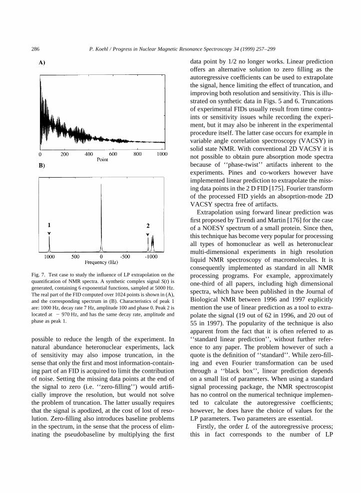
where {W} is the DFT of the noise sequence {w};{ W} is a white noise process in the spectral domain[41]. The first term on the right side of Eq. (76) is asum of complex Lorentzian functions. In the simplecase in which allw k are zero, the real part of thespectrum described by Eq. (76) will appear as thesuperposition of pure absorption Lorentzians,centered at the characteristic frequenciesfk, of ampli-tudeck/Rk, linewidth at half heightRk and surfaceck. Inthe more general case in which the phase parametersare non-zero, the spectrum is first ‘‘phased’’ prior toany quantitative analysis, i.e. a correction factor of theform exp(2 jf i) is applied to each spectral pointFI,which restores the pure absorption appearance for thereal part of the spectrum. A general scheme forextracting information such as intensities from NMRsignals has been accordingly defined, which includesapodization of the FID (to remove artifacts because offinite size samples as well as to improve the SNR),spectral analysis through Fourier transformation,phasing and baseline correction of the frequency-domain spectra (baseline offset in the spectral domainusually results from corruption in the first data pointof the FID), and quantification through peak-pickingand numerical integration. Limitations of this proce-dure appear however for signals with low signal-to-noise ratio, as well as in crowded or complicated spec-tra which show severe overlaps. In these cases, wehave to look for alternative solutions.
Direct fitting of Eq. (75) to noisy experimental dataleads to a difficult nonlinear least-squares problem,which requires thatK be known, as well as good initialvalues for all spectral parameters [41]. Methods tosolve this nonlinear problem have been mainly imple-mented as a final refinement procedure, after initialguesses for all or some of the parameters have beenderived using another technique (which could be FTand visual inspection of the spectrum, when all peakscan be clearly identified) [139–143]. Fitting in thespectral domain has the same problems.
Maximum entropy [46] is a non-parametricapproach whose aim is to enhance the signal contentin a reconstructed spectrum. As such, it does not
directly provide quantitative information on thesignal, though this is an area in development now[52]. It should be noted here that there have beensome ambiguities in the literature about the use ofthe term ‘‘maximum entropy’’. The Burg algorithmis sometimes referred to as maximum entropy, thoughit is an AR procedure. There is also a maximumentropy regularization procedure, though to myknowledge, it has not been applied to linear predic-tion. The maximum entropy technique mentionedhere performs a nonlinear least-squares fit of amodel signal to the experimental spectrum, underthe constraint that the ‘‘entropy’’ of the signal shouldbe minimal. Daniell and Hore provide a nice explana-tion of the significance of this entropy term [49].
Linear prediction in its model-based definition hasattracted considerable interest as a quantitative alter-native to FT analysis. It includes the following threesteps:
1. Firstly, the NMR signal is considered to be an ARprocess, and the linear coefficients {b} arecomputed, using one of the techniques presentedearlier.
2. Once the {b} are known, the frequenciesfk and therelaxation ratesRk of the signal can be calculatedfrom the complex rootsZk of the characteristicpolynomial defined by:
P�z� �XPm�0
bmzP2m �77�
whereP is the order chosen for the AR process, andb0 � 1. Eq. (77) is directly derived from Eq. (30),while the relation between the roots and thefrequencies and damping factors is described byEq. (28).
3. Finally, the complex amplitudesckejwk are deter-
mined from Eq. (75) in the modified form
An �XPk�1
ckejwkzn
k 1 wn �78�
by a least squares calculation.
It is worth noting here that the sum in Eq. (75) hasbeen extended fromK, the true number of exponen-tials, toP, the presumed order of the AR process.
Procedures for deriving the AR coefficients havebeen described at length in the preceding sections.
P. Koehl / Progress in Nuclear Magnetic Resonance Spectroscopy 34 (1999) 257–299 275
We will therefore concentrate here on the root findingprocedure required in step 2, as well as on the LSQcalculation of step 3.
4.2. Extracting the frequencies and decay rates
4.2.1. Roots of the characteristic polynomialConsidering that at this stage the linear coefficients
{ b} have been computed, the next step is to calculatethe roots of the polynomial given by Eq. (77), fromwhich the frequencies and amplitudes of the signalcomponents can be derived based on Eq. (78). Severalmethods exist to find the roots of a polynomial,including an algorithm proposed by Steiglitz andDickinson [144] which has been used for LP byBarkhuisen et al. [65,66] and by Tang et al.[65,66,96] as well as the algorithm proposed by Svej-gard [145] which is used by Gesmar and co-workers[41,95]. The latter procedure performs linearly withthe order of the polynomial and is robust, making it agood option for high order LP calculations. Anotherapproach [146] is to transform the root finding stepinto an eigenvalue problem. Any polynomial equationof the form:
P�x� �XNi�0
aiXi � 0 �79�
can be recast into the problem of finding the eigenva-lues of the (N 1 1) × (N 1 1) matrix:
A �
0 0 : : 2a0
1 0 : : 2a1
0 1 0 : 2a2
: : : : :
0 0 : 1 2aN
26666666664
37777777775�80�
as P(x) is the characteristic polynomial ofA, i.e.P�x� � det�A 2 xI � whereI is the identity matrix ofsize (N 1 1) × (N 1 1). It should be noticed howeverthat A has no special structure, in which case theeigenvalue problem cannot be simplified. In the caseof high polynomial order, it also suffers from highrequirements in computer memory usage.
Polynomial rooting can also be avoided using thestate–space models: this will be described later.
All procedures aforementioned rely on the fact thatthe linear prediction orderP is much larger than the
true number of exponential functions contained in thesignal. IncreasingP however results in a large numberof extraneous roots for the polynomial. The problemof distinguishing these roots from true signal-relatedroots has been discussed by many authors, with majorcontributions from Kumaresan and Tufts [147,148].Briefly, in the case of forward linear prediction, allroots fall within the unit circle in the complex plane.However, in the case of backward linear prediction,signal-related roots will fall outside the unit circle,while extraneous roots will fall both inside andoutside the unit circle: all roots falling inside the circlecan usually be discarded.
The distinction of signal roots from noise rootsbased on their relative position with respect to theunit circle in the complex plane becomes difficultfor signals with low signal-to-noise ratios: even inthe case of backward prediction, signal roots canmove inside the unit circle, while noise roots moveoutside. Delsuc et al. [149] have tried to overcome thisproblem using a method suggested by Porat and Fried-lander [150]. Basically the method relies on the factthat the same signal roots should be found in forwardLP and in backward LP after reflection inside the unitcircle, while noise roots should not be related to eachother. The method calculates the pairwise distancesbetween roots obtained from the two types of LP,and signal roots are defined as those for which thedistance is minimum. An estimate of the exact numberof signal roots is needed.
Zhu and Bax [151] proposed an alternative way touse the information contained in the backward andforward LP coefficients. As mentioned earlier, theroots derived from forward coefficients and thosederived from backward prediction should be identical,after reflection within the unit circle of the latter.These sets of roots can be used to recalculate twosets of LP coefficients. In the presence of noise,these two new sets of coefficients will be different,and Zhu and Bax [151] proposed to reduce the contri-bution of the random errors induced by noise bysimply averaging the two sets of coefficients. Newroots are then computed based on the average coeffi-cients.
NMR studies of macromolecules in solution gener-ate signals with a high number of exponential func-tions. We have seen earlier that LP techniques requirethat the number of poles defined in the calculation be
P. Koehl / Progress in Nuclear Magnetic Resonance Spectroscopy 34 (1999) 257–299276
much larger than the true number of peaks. Thecombination of these two conditions requires thatvery high degree polynomial equation be solved inorder to get the characteristic frequencies and relaxa-tion rates of the nuclei of the macromolecule understudy (Gesmar and Hansen [137] have published acase with a polynomial order of 16 000). The largeexponents in the polynomial require special care inorder to avoid computing overflows. Fortunately, inthe case of high resolution NMR, the roots of thepolynomial fall very close to the unit circle in thecomplex plane. A stable strategy to solve high orderpolynomial equations of the formP(z) � 0 wasdescribed by Svejgard [145], in which roots arefound iteratively by searching for minima ofuP(z)u,directing the search away when an overflow occurs.When a root is found, the polynomial is deflated, andthe procedure is repeated up to the last root. With theintroduction of fast techniques to solve for the coeffi-cients, solving for the roots of the characteristic equa-tion has become the time limiting step in quantitativeNMR.
4.2.2. Avoiding polynomial rooting: The state–spacemodels
Barkhuijsen et al. [152] proposed an alternativemethod to directly extract the poles of the signalwhich makes use of the Hankel structure of the matrixas well as of the exponential nature of the signal. Wewill give a brief description of this method.
The NMR signal is modeled by a sum of dampedexponential functions, as described by Eq. (26). Thisequation can be rewritten in matrix form:
A1
A2
:
:
AN21
26666666664
37777777775�
1 1 : : 1
Z1 Z2 : : ZK
: : : : :
: : : : :
ZN211 ZN21
2 : : ZN21K
26666666664
37777777775
c1
c2
:
:
cK
26666666664
37777777775�81�
where theZi are the poles, defined by Eq. (27), andcthe amplitude. Eq. (69) is a good illustration that theproblem of extracting the components of a signal canbe broken down into first finding its poles, and thenthe complex amplitudes.
Eq. (81) can be applied to each column of the
complete data matrix (in Hankel from) from whichwe derive:
H �
1 1 1 1 1
Z1 Z2 : : ZP
: : : : :
: : : : :
ZN2P1 ZN2P
2 : : ZN2PP
26666666664
37777777775
�
c1 c1Z1 : : c1ZP211
c2 c2Z2 : : c2ZP212
: : : : :
: : : : :
cP cPZP : : cPZP21P
26666666664
37777777775�82�
or
H � ZC �83�H is the Hankel data matrix,Z is the matrix
containing the pole, andC a mixed matrix containingboth poles and amplitudes. The aim is to propose amethod to extractZ, based onH, and then to extractthe individualZi, based on the matrixZ.
Another decomposition ofH can be obtained fromits singular value decomposition:
H � UDV* � UV 0 �84�whereV 0 combinesD andV*.
Replacing Eq. (83) in (84), we obtain:
Z � UVC21 � UQ �85�whereQ � V 0C21.
Z has the special form of a Vandermonde matrix. Inthat respect, it has the general property that any twosubsets of the same size of its rows share the samesubspace. For example, if we callZ l andZ f the twosub-matrices obtained by removing the last and firstrow, respectively, it is easy to see that they verify:
Z l � ZfG �86�whereG is the diagonal matrix defined by:
G � Diag{Z1;Z2;…;ZP} :
If we define in the same wayUl and Uf as the sub-matrices ofU in Eq. (85) in which the last and first
P. Koehl / Progress in Nuclear Magnetic Resonance Spectroscopy 34 (1999) 257–299 277
rows are missing, respectively, Eq. (85) yields
Z l � UlQ and Zf � Uf Q �88�Combining Eq. (86) and (88), we obtain:
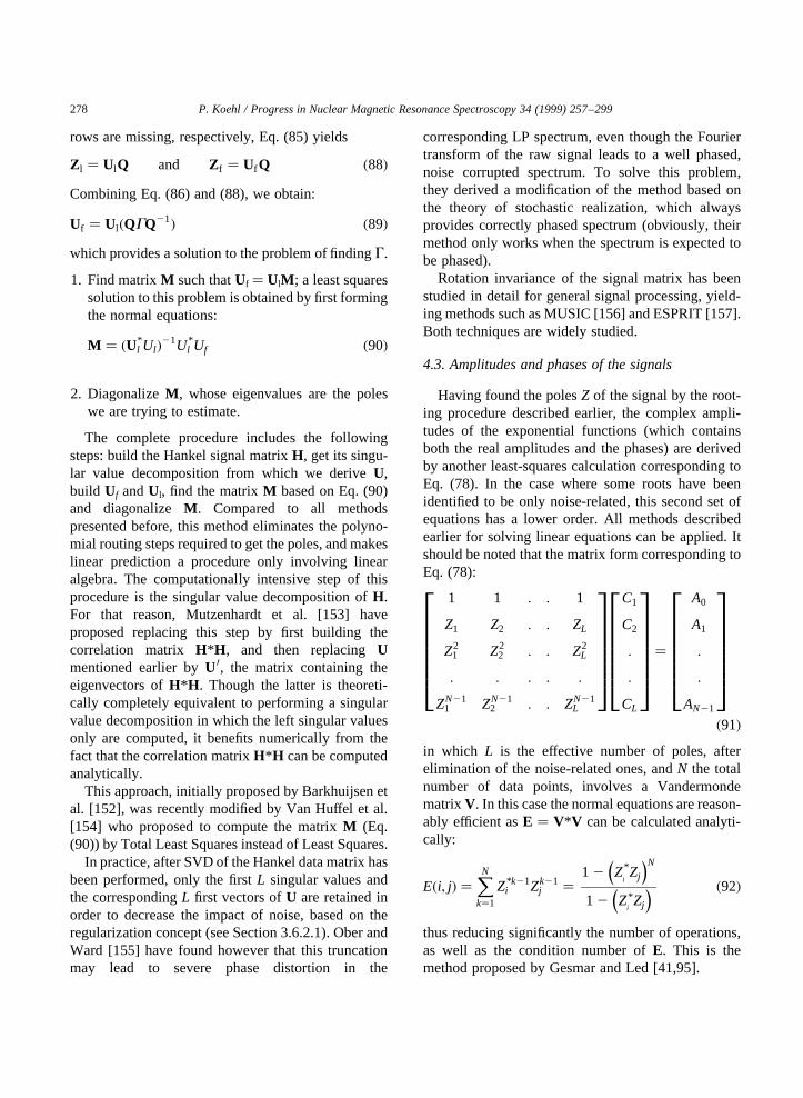
Uf � Ul�QGQ21� �89�which provides a solution to the problem of findingG.
1. Find matrixM such thatUf � UlM ; a least squaressolution to this problem is obtained by first formingthe normal equations:
M � �U*l Ul�21U*
l Uf �90�
2. DiagonalizeM , whose eigenvalues are the poleswe are trying to estimate.
The complete procedure includes the followingsteps: build the Hankel signal matrixH, get its singu-lar value decomposition from which we deriveU,build Uf andUl, find the matrixM based on Eq. (90)and diagonalize M . Compared to all methodspresented before, this method eliminates the polyno-mial routing steps required to get the poles, and makeslinear prediction a procedure only involving linearalgebra. The computationally intensive step of thisprocedure is the singular value decomposition ofH.For that reason, Mutzenhardt et al. [153] haveproposed replacing this step by first building thecorrelation matrix H*H, and then replacingUmentioned earlier byU 0, the matrix containing theeigenvectors ofH*H. Though the latter is theoreti-cally completely equivalent to performing a singularvalue decomposition in which the left singular valuesonly are computed, it benefits numerically from thefact that the correlation matrixH*H can be computedanalytically.
This approach, initially proposed by Barkhuijsen etal. [152], was recently modified by Van Huffel et al.[154] who proposed to compute the matrixM (Eq.(90)) by Total Least Squares instead of Least Squares.
In practice, after SVD of the Hankel data matrix hasbeen performed, only the firstL singular values andthe correspondingL first vectors ofU are retained inorder to decrease the impact of noise, based on theregularization concept (see Section 3.6.2.1). Ober andWard [155] have found however that this truncationmay lead to severe phase distortion in the
corresponding LP spectrum, even though the Fouriertransform of the raw signal leads to a well phased,noise corrupted spectrum. To solve this problem,they derived a modification of the method based onthe theory of stochastic realization, which alwaysprovides correctly phased spectrum (obviously, theirmethod only works when the spectrum is expected tobe phased).
Rotation invariance of the signal matrix has beenstudied in detail for general signal processing, yield-ing methods such as MUSIC [156] and ESPRIT [157].Both techniques are widely studied.
4.3. Amplitudes and phases of the signals
Having found the polesZ of the signal by the root-ing procedure described earlier, the complex ampli-tudes of the exponential functions (which containsboth the real amplitudes and the phases) are derivedby another least-squares calculation corresponding toEq. (78). In the case where some roots have beenidentified to be only noise-related, this second set ofequations has a lower order. All methods describedearlier for solving linear equations can be applied. Itshould be noted that the matrix form corresponding toEq. (78):
1 1 : : 1
Z1 Z2 : : ZL
Z21 Z2
2 : : Z2L
: : : : :
ZN211 ZN21
2 : : ZN21L
26666666664
37777777775
C1
C2
:
:
CL
26666666664
37777777775�
A0
A1
:
:
AN21
26666666664
37777777775�91�
in which L is the effective number of poles, afterelimination of the noise-related ones, andN the totalnumber of data points, involves a VandermondematrixV. In this case the normal equations are reason-ably efficient asE � V*V can be calculated analyti-cally:
E�i; j� �XNk�1
Z*k21i Zk21
j �1 2 Z*
iZj
� �N
1 2 Z*iZj
� � �92�
thus reducing significantly the number of operations,as well as the condition number ofE. This is themethod proposed by Gesmar and Led [41,95].
P. Koehl / Progress in Nuclear Magnetic Resonance Spectroscopy 34 (1999) 257–299278
Noise or glitches in the first data points of theexperimental NMR signal yield to an offset in thespectrum after Fourier transformation as well as tobaseline distortion, which makes least squares analy-sis of the spectrum difficult. The first points howevercannot be removed prior to Fourier analysis, or largephase problems occur. In the LP procedure however,the first points can be omitted both for finding the LPcoefficients, and for the calculation of the amplitudesdescribed earlier.
4.4. Conclusions on model-based analysis of NMRsignals
The NMR FID can be modeled as the sum ofcomplex exponential functions. Finding the character-istic elements of the signal components by nonlinearleast-squares minimization is a hard numericalproblem, which requires knowledge of good initialconditions which are not readily available in thecase of complex signals. Under reasonable assump-tions however, the digital experimental signalsampled at constant time interval can be defined asan AR process. The problem of solving for the ampli-tudes and phases of the exponential functions can thenbe solved by a method known as the extended Pronymethod which consists of three basic steps. Firstly, theAR coefficients are determined, which are used todefine a characteristic polynomial. The second stepinvolves finding the roots of this polynomial, fromwhich the frequencies and damping factors of thecomponents of the NMR signal are derived. Theseroots are also used in the final procedure which eval-uates the complex amplitudes of the signal using aleast squares approach.
Several methods have been proposed to find theroots of the AR polynomial. One of the major issuesdealt with by these methods is the problem of poten-tial overflow as a result of the high orders involved.Fortunately, all signal roots fall very close to the unitcircle in the complex plane. Solving for the roots ofthe characteristic polynomial is the only nonlinearstep in the whole procedure. It can be recast into aneigenvalue problem using the companion matrixapproach, or even completely bypassed using thestate–space approach proposed by Barkhuijsen et al.[152] which combines the two approaches.
The final step involves solving a linear system to
extract the complex amplitudes of the exponentialfunctions which describe the signal. Several linearleast-squares techniques are available to solve thisproblem; it is worth noting that the normal equationsare a reasonable solution as they can be built analyti-cally, instead of involving the costly product of twomatrices (both in time and precision).
5. Linear prediction applied to ND NMRexperiments
The development of NMR for solving solutionstructures of macromolecules has greatly benefitedfrom the successive introductions of multi-dimen-sional NMR techniques (2D in the 1970s, 3D andeven higher since then) [5,9,10,12,158]. Dimensionsin an ND NMR experiments are not equivalent: in thedetected dimension, long acquisition times can beused without adding to the total time needed forrecording the spectrum, while in the indirectlydetected dimensions, acquisition time is kept small,and usually shorter than the macroscopic relaxationrateT2. Limitations are mainly related to the fact thatthere are constraints of time as well as storage forrecording these types of experiments. As signalsacquired for longti values contribute less to thesignal-to-noise ratio, whereti corresponds to one ofthe reconstructed dimension, the totalti time is usuallykept shorter thanT2.
Truncation of a time-domain signal is a problem inthe case of a Fourier analysis, and zero-fillingfollowed by severe apodization only offers a partialsolution. In the case of 1D experiments, we haveshown that linear prediction offers an alternative solu-tion, using the autoregressive properties of the signal;it should therefore also provide an effective improve-ment of ND experiments. LP is a time-consumingprocedure though, and simplifications and/or short-cuts are usually needed to keep the computation fora ND experiment tractable.
5.1. Extracting amplitudes from a ND spectrum
The simpler solution is to extract as much informa-tion as possible prior to analysing the ND experiment.This was originally proposed by Manassen et al. [159]for a 2D experiment: they first determined the reso-nance frequencies and the decay rates of the spins of
P. Koehl / Progress in Nuclear Magnetic Resonance Spectroscopy 34 (1999) 257–299 279
the sample under study from a well resolved 1Dexperiment, and then calculated the amplitude of the2D signals by a least-squares calculation. The sameprocedure was rediscovered 10 years later by Muller[160].
It should be mentioned that this method would notbe reliable in the case of complicated spectra showingsevere signal overlap in 1D experiments (for whichhigher dimensional experiments are usually requiredto resolve the overlaps).
5.2. Hybrid spectral analysis for ND spectra
The most common applications of linear predictionto 2D experiments uses the fact that multidimensionalFourier transform is separable, i.e. each dimensioncan be treated independently [34]. In fact, there isno need to use the same technique for spectral analysisin each dimension: for example, DFT could be appliedto the detected dimension, as it usually containsenough data points, while a high-resolution modelingmethod could be used afterwards for any of the recon-structed dimensions. This leads to the concept ofhybrid spectral analysis. All techniques presentedbefore for 1D signal are then adequate, leading tothree different approaches:
1. After DFT has been applied to the detected dimen-sion, each FID in the reconstructed dimension isextended by linear prediction prior to Fourier trans-form: this minimizes the need for strong apodiza-tion, and should therefore improve both sensitivityand resolution. Such techniques have been appliedto 2D, 3D and 4D data matrices [32,33,41,68,161].It should be mentioned that in 3D and 4D, thetruncation problem is unavoidable, to the extentthat in some of the indirectly detected dimensions,only 8 or 16 time increments are used. These caseshighlight another problem, i.e. the fact that thenumber of correlations present in a given dimen-sion can exceed the number of data points avail-able. Zhu and Bax [162] have proposed anelaborate procedure to account for this problem:in the case of a 2D experiment for whicht2 andt1 are the detected and indirectly detected dimen-sions, respectively, they use a sequence composedof Fourier transformation int2, followed byextrapolation by linear prediction of all FID int1,then FT in t1, inverse Fourier transform int2,
extrapolation by linear prediction int2, and finallyFT in t2.
2. The first approach described before only uses theautoregressive properties of the signal to extrapo-late the FID, and then applies DFT. We have seenin the preceding sections that spectral analysis canbe performed based solely on the fact that thesignal is an AR process: this has been used byHoch [163] for a 2D COSY spectrum in a techni-que that can be referred to as ‘‘hybrid 2D spectralestimator’’, in which 1D DFT in the detecteddomain t2 is followed by spectral estimation inthe t1 or indirectly detected dimension. He usedBurg’s algorithm to calculate the AR coefficientsfrom which he derived a power spectrum based onEq. (19). The final hybrid spectrum showed higherresolution compared to a 2D spectrum generatedby FT in the two dimensions on the same amountof data.
3. Linear prediction can also be used quantitatively toderive directly all components of the signal. Schus-seim and Cowburn [164] have used this propertyfor the hybrid spectral analysis of a 2D signal, byfirst applying DFT in thet2 dimension, followed byquantitative LP analysis int1. Application of theextended Prony method yields lists of signal para-meters for each column of the data matrix, andthese lists can be scanned to filter for true signalsand to eliminate noise.
Hybrid spectral analysis does not have toinclude DFT: linear prediction could be appliedin dimension 2, followed by nonlinear least-squares modeling in dimension 1. This strategywas applied to the quantitative determination ofthe exchange rates of slowly exchanging amideprotons in proteins [165]. In this study, theexchange rates are obtained by fitting a modelthat includes exponential decay (i.e. NLSQ in apseudo-dimension 1) to the parameters producedby a linear prediction analysis of a series of 1DFID recorded during the exchange of the amideprotons with solvent (LP in dimension 2). LP analysisof each FID requires a large number of LP coefficientsin order to assure a correct estimate of the spectralparameters and this calculation must be repeated foreach FID. This was made possible using the fast LPprocedure of Gesmar and Hansen [137].
P. Koehl / Progress in Nuclear Magnetic Resonance Spectroscopy 34 (1999) 257–299280
5.3. Spectral analysis using sequential linearprediction
The hybrid procedure aforementioned can beextended one step further, in the sense that bothdimensions can be analyzed by a high-resolutionmodeling technique. This was initially proposed byBarkhuijsen and coworkers for 2D electron spin data[65], and then modified by Gesmar and Led [166] tocomply with NMR data. In the following, we describethe latter technique.
Let us consider a 2D experiment in which thedata are complex in both dimensions. The corre-sponding 2D can be expressed as a sum of bi-complex signals under the three conditions thatthe experiment can be phased in absorptionmode, there is not first-order phase correction inone of the dimension, and the noise contributioncan be neglected [167]. Most of the phase-sensi-tive experiments satisfy these conditions, provid-ing that the experimental conditions are definedsuch that the detected dimension requires very littlefirst order correction. The general expression for anhypercomplex FID is:
x�t1; t2� �XKk�1
XLl�1
Ckl�exp�iw�1�
k
�� exp
�jw�2�
l
�exp
�2 R�1�
kt1�exp
�i2pf �1�
kt1�
� exp�
2 R�2�l
t2�exp
�j2pf �2�
lt2�
�93�
in which modulation occurs in the two dimensionsdefined by t2 and t1. Ckl is the real amplitude ofthe correlation between peakk and l, w stands forthe phase,R for the decay rate, andf for thefrequency of resonance. The superscripts 1 and 2indicate that the quantity is related witht1 and t2,respectively. For sake of clarity, we differentiatethe number for complex representation in the twodimensions, and denote them asi and j. x(t1,t2)corresponds in fact to two complex numbers orfour real numbers which are usually referred toas rr, ir, ri and ii where r stands for real and i forimaginary.
When this signal is sampled at regularly spacedintervals in the two dimensions, it can be represented
by an hypercomplex time series:
Amn�XKk�1
Bmkexp�jw�2�
k
�� exp
�2 R�2�
knD2
�exp
�j2pf �2�
knD2
�1 wmn �94�
where
Bmk�XLl�1
Cklexp�iw�1�
l
�� exp
�2 R�1�
lmD1
�exp
�i2pf �1�l mD1
� �95�D1 andD2 are the sampling interval in thet1 andt2dimensions, respectively, andw the noise sequence.Aandw have hypercomplex values which depend oniandj, while B is complex, and depends oni only. Theconcept of hypercomplex representation might beconfusing at this stage and should be seen simply asa condensed mathematical notation. What happens isthat in the case of a States experiment [168], two FIDSare recorded for eacht1 time value, i.e. for eachm,with a phaseshift between the two ofp /2. A singlecompact model for these two FIDs is directly encodedinto Eq. (94), which can be decomposed into standardcomplex notation as:
Ar�2m21�n �
XKk�1
real�Bmk�exp�jw�2�
k
�� exp
�2 R�2�
knD2
�exp
�j2pf �2�
knD2
�1 wr
�2m21�n
�96�and
Ai�2m�n �
XKk�1
imag�Bmk�exp�jw�2�
k
�� exp
�2 R�2�
knD2
�exp
�j2pf �2�
knD2
�1 wi
�2m�n
�97�in which 2m 2 1 and 2m refer to the FID index, andAr, Ai, wr, wi are standard complex numbers.
Eqs. (96) and (97) relate to thet2 or detecteddimension, while Eq. (95) corresponds to the recon-structed dimension. This separation provides the basisfor the sequential LP spectral analysis techniqueproposed by Gesmar and Led [166], which schemati-cally proceeds as follows:
P. Koehl / Progress in Nuclear Magnetic Resonance Spectroscopy 34 (1999) 257–299 281
1. A model-based linear prediction procedure isapplied on each FID, yielding the frequencies anddecay rates in thet2 dimension, as well as theamplitudes defined as real(B) and imag(B).
2. For each frequencyk in dimension 2, a complexFID is reconstructed in dimension 1, based on Eq.(95).
3. Each reconstructed FID is analyzed by quantitativelinear prediction, yielding the frequencies anddecay rates in dimension 1, as well as the ampli-tudesC of the correlation between the frequencies.
Performing LP on each FID of the 2D data set canbe very costly in computer time; however this proce-dure can be greatly simplified. In Eqs. (96) and (97),the two exponential expressions which contain thedecays rates and the frequencies are independent ofm, consequently the linear coefficients are indepen-dent of m. The entire two-dimensional data set cantherefore be included in the determination of the coef-ficients for thet2 dimension. Gesmar and Led [166]proposed to generate the matrix corresponding to thetotal set of normal equations by summing the normalequation matrices built from each FID. Having foundthe autoregressive coefficients based on this cumula-tive data matrix, the poles of the signal in thet2dimension are derived as the root of the characteristicequation, from which the frequenciesf(2) and decayratesR(2) are extracted.
As the poles are known at this point, the amplitudesB are evaluated using a LSQ procedure. This calcula-tion must be carried out for each FID, though theinversion of the matrix required to solve the systemsneed only be performed once.
The simplification proposed earlier for thet2dimension could be applied theoretically for thet1dimension also. However, Gesmar and Led [166]preferred to perform the complete LP calculationsindependently for each reconstructed FID in dimen-sion 1. The main reason behind this choice is that thenumber of available data points in thet1 dimension isusually small, which limits the choice for the linearprediction order; the latter however should be chosento be larger than the expected number of resonance inthe signal, in order to comply with the autoregressivemodel (see Section 3). In most cases, each resonancein the t2 dimension is only correlated with a smallnumber of frequencies, and a small LP order is
sufficient. Including all possible frequencies howeverwould require a much larger number of data points.
Let us defineZ(1) andZ(2) by:
Z�2�k � exp 2R�2�k D2
h iexp j2pf �2�k D2
h iZ�1�l � exp 2R�1�l D1
h iexp j2pf �1�l D1
h i �98�
and let us consider the special case where the signal is‘‘symmetric’’ with respect to the two frequency axes,and the sample intervals for the two time axes are thesame. Under these conditions, allZ(1) andZ(2) are theelements of the same listL, i.e. the same list of poles isexpected in both dimensions. Under these restrictiveconditions, there exists a set of AR equations satisfiedby the signal in both dimensions. From these equa-tions, a set of AR coefficients is derived, and used tobuild the characteristic polynomial whose roots corre-spond toL, the list of Z values defined earlier. Theknowledge of these poles allows the calculation of thefrequencies and corresponding decay rates of thesignal, as well as the amplitude of the correlation,based on a least-squares calculation. This is the strat-egy proposed by Imanashi et al. [169], which can beseen as an extension of the method of Gesmar and Led[166].
The two major challenges in the estimation of 2Dsignal intensities are the handling of signal overlapsand the accurate definition of a base plane for thesignals to be examined. While overlaps can behandled directly by both methods described earlier,the baseline may be more of a problem. This is animportant issue for signals recorded on samples inH2O solutions, in which cases the spectra show severedistortion of the baseline caused by the dispersive tailsfrom the water resonance (‘‘F2 ridges’’). As shown byHolak et al. [170], the intensityI of the correlationbetween two frequenciesf1 andf2 in a phase-sensitive2D spectrum can be estimated from the product of the1D intensities,I2(f1) andI1(f2), as determined from therow atf� f1 and the column atf� f2, respectively, andfrom the spectrum amplitudeS(f1,f2), using:
I � I2�f1�I1�f2�S�f1; f2� �99�
Within this framework, Gesmar et al. [171] designedan alternative approach based on sequential applica-tion of linear predictions in both dimensions of the 2D
P. Koehl / Progress in Nuclear Magnetic Resonance Spectroscopy 34 (1999) 257–299282
signal. In this method, the 1D intensitiesI2(f1) andI1(f2) are determined independently by linear predic-tion, followed by nonlinear least-squares analysis,after whichS(f1,f2) is calculated from the estimatedspectral parameters. This method will fail in thepresence of large baseline distortion, but can easilyaccommodate a baseline correction. Such a modifica-tion was suggested by Kristensen et al. [172] whichproceeds as follow: the 1D intensityI2(f1) is deriveddirectly from the partially Fourier transformed datasetS(t2,f1), as originally proposed by Gesmar et al. [171].To enable a linear prediction in the F1 dimension on abaseline corrected signal, the 2D data setS(t1,t2) isFourier transformed and phase corrected in bothdimensions, then a baseline correction is performedin the F2 dimension, and finally an inverse Fouriertransform reverts the F1 dimension to the timedomain, to give the required data setS(f2,t1), fromwhich an apparent intensityI1*( f2) is derived. At thispoint, it is important to realize that the baselinecorrection in the F2 dimension affects the estimated1D intensity in the F1 dimension, and thatI1(f2) ±I1*( f2). This comes from that fact that the discreteFourier transform of an exponentially damped sinu-soid can be approximated as the sum of a Lorentzianand a pseudo-baseline [41]. By removing the baselinein the 2D spectrum, both the ridges and the pseudo-baseline for each column of the matrix have beenremoved. The latter can be accounted for when
estimating the F1 1D signal intensity by setting:
I1�f2� � I *1�f2�1 Ib2 �100�
whereI is the intensity of the correlation betweenf1and f2, andb2 the F2 pseudo-baseline level. The 2Dintensity I is then derived by replacing Eq. (100) inEq. (99), and solving forI.
5.4. Direct 2D LP analysis
Both the hybrid procedure as well as the sequentialLP method described earlier make use of the separ-ability of spectral analysis of multidimensional data.The concept of direct 2D LP spectral analysis of NMRspectra has been suggested originally by Marple [70]and by Kumerasan and Tufts [173], and exploited forthe first time by Zhu and Bax [174]. The latter authorsproposed to replace the general equation for 1D auto-regression by two master equations in 2D, which are:
x�m;n� �XMk�1
XP2 1
l�0
cklx�m2 k;n 2 l� �101�
and
x�m;n� �XM 2 1
k�0
XPl�1
dklx�m2 k; n 2 l� �102�
where x is the hypercomplex signal,M and P thelinear prediction order in dimensions 1 and 2,
P. Koehl / Progress in Nuclear Magnetic Resonance Spectroscopy 34 (1999) 257–299 283
Fig. 4. Schematic representation of the LP procedure of Zhu and Bax [174] for extrapolation of 2D NMR signals. Extrapolation in dimension 1defined by Eq. (101) is described. Experimentally determined data points are shown as circles (W), while extrapolated points are shown as (1 ).(A) The experimental signal is causal in both dimensions, restricting the extrapolation: for example, with the LP order considered [(M,P) �(3,3)], the data points at (0.5,6.5) and (1.5,6.5) cannot be computed. A solution to this problem was proposed by Zhu and Bax, in which thesignal is first extrapolated in the negative time domain by reflection (data points shown as *), as shown in (B).
respectively, andckl anddkl two sets of linear coeffi-cients. When using Eq. (101), the data matrix can beextended in dimension 1 only, while Eq. (102) allowsextension in dimension 2, as illustrated in Fig. 4.
Based on Eq. (101), it is only possible to predictx(m,n) for which n . P: for example, all data pointsx(N1 1 1,n) cannot be predicted ifn , P. To cir-cumvent this limitation, Zhu and Bax [174] haveproposed extending the data in the negative time-domain first, and then apply the 2D LP procedure,as shown schematically in Fig. 4. Extension into thenegative time-domain is performed as follows. First,as the time-domain is short, it is possible to assume, asa first approximation, the decay rates to be the samefor all frequency components, in which case thedamping of the signal can be remove by multipli-cation by a single increasing exponential. Afterremoval of the decreasing component, the signalcan be extended into the negative time-domain bysimple symmetry. To avoid discontinuity, the
phase of the signal has to be adjusted experimentallyto zero at time zero, and the first data point is set toexactlyD/2.
This method was found to work better than thehybrid FT-LP procedure based on the separability ofthe spectral analysis on 2D data that are severely trun-cated in both dimensions. In practice, this method isonly of real use for the analysis of 3D or 4D data sets.The price in computing time of this method ishowever enormous. Zhu and Bax [174] mentionedin their paper that application of this procedure to asmall 16× 16 hypercomplex data matrix using a 12×12 hypercomplex prediction matrix required 20 minon a 10 Mflops computer. Considering that the proce-dure has to be applied twice for extension in bothdimension, and repeated for all cross sections througha 3D and 4D data set, the total computational timerequired limits its application. To our knowledge,there has not yet been any follow-up to the paper ofZhu and Bax [174].
P. Koehl / Progress in Nuclear Magnetic Resonance Spectroscopy 34 (1999) 257–299284
Fig. 5. A synthetic FID corresponding to a signal containing 4 components at frequencies2 1000, 2 985, 2 970 and2 900 Hz. All signalshave the same decay rates (7 Hz), same amplitude (100), and same phase (0). The synthetic FID is sampled at 200ms, and a white noisesequence is added, with a SNR of 30 dB. (a) real part of the complete FID over 1024 points. (b) real part of the FID truncated after 256 points. (c)same as in (b), after exponential apodization (lb� 10Hz). (d) the truncated FID shown in (b) is extrapolated by linear prediction up to originalsize of 1024 data points. The linear coefficients are computed based on a SVD of the data matrix, including all 256 available data points, with aLP order of 128.
6. Linear prediction analysis of NMR spectra
As we have seen before, the name ‘‘linear predic-tion’’ in the field of NMR spectroscopy covers twodifferent types of applications:
1. The NMR signal can be modeled as an autoregres-sive process, and the AR coefficients can be usedeither to extrapolate the time domain signal, or toconstruct a spectrum;
2. A complete quantitative spectral analysis of theNMR signal is performed based on the AR coeffi-cients and a mathematical model for the signal,using the so-called extended Prony method.
The next two sections cover examples of these twoapplications, as well as a discussion of their limita-tions.
6.1. Linear prediction can complement Fouriertransformation
The NMR free induction decay signal is measured
at N intervals of time to give the data vectorfAngn� 0;…;N 2 1. Provided that the time interval isconstant, this time series can be analyzed by applica-tion of the discrete Fourier transform. DFT providesas output a spectrum, from which information on thespin system can be derived, such as resonancefrequencies, relaxation rates and population (intensi-ties). However, DFT has strict requirements as well aslimitations, and some of these can be alleviated bylinear prediction.
The FID is acquired over a finite time interval,D�ND. The corresponding truncation results in distor-tions in the signal, i.e. ‘‘wiggles’’ which appear onboth side of each frequency component. The totalacquisition time is also inversely proportional to thespectral resolution. Both conditions call for FIDs witha large number of data points covering most of thetransient physical signal. This is usually not a problemfor 1D NMR as data points can be collected withoutany cost; in the case of high dimensional NMRhowever, the number of measurements in any of thereconstructed dimensions should be kept as low as
P. Koehl / Progress in Nuclear Magnetic Resonance Spectroscopy 34 (1999) 257–299 285
Fig. 6. (a), (b), (c) and (d) show the real part of the FT spectra corresponding to the signals shown in Figs.5(a),(b),(c)and(d), respectively.Truncation of the signal induces a loss of resolution, as well as the apparition of ‘‘wiggles’’ on the spectrum, as shown in (b). Apodization withan exponential function removes the wiggles as well as reduces the contribution of noise, at the cost however of a loss of resolution (see (c)). Byextrapolation using linear prediction, the resolution is recovered.
possible to reduce the length of the experiment. Innatural abundance heteronuclear experiments, lackof sensitivity may also impose truncation, in thesense that only the first and most information-contain-ing part of an FID is acquired to limit the contributionof noise. Setting the missing data points at the end ofthe signal to zero (i.e. ‘‘zero-filling’’) would artifi-cially improve the resolution, but would not solvethe problem of truncation. The latter usually requiresthat the signal is apodized, at the cost of lost of reso-lution. Zero-filling also introduces baseline problemsin the spectrum, in the sense that the process of elim-inating the pseudobaseline by multiplying the first
data point by 1/2 no longer works. Linear predictionoffers an alternative solution to zero filling as theautoregressive coefficients can be used to extrapolatethe signal, hence limiting the effect of truncation, andimproving both resolution and sensitivity. This is illu-strated on synthetic data in Figs. 5 and 6. Truncationsof experimental FIDs usually result from time contra-ints or sensitivity issues while recording the experi-ment, but it may also be inherent in the experimentalprocedure itself. The latter case occurs for example invariable angle correlation spectroscopy (VACSY) insolid state NMR. With conventional 2D VACSY it isnot possible to obtain pure absorption mode spectrabecause of ‘‘phase-twist’’ artifacts inherent to theexperiments. Pines and co-workers however haveimplemented linear prediction to extrapolate the miss-ing data points in the 2 D FID [175]. Fourier transformof the processed FID yields an absoprtion-mode 2DVACSY spectra free of artifacts.
Extrapolation using forward linear prediction wasfirst proposed by Tirendi and Martin [176] for the caseof a NOESY spectrum of a small protein. Since then,this technique has become very popular for processingall types of homonuclear as well as heteronuclearmulti-dimensional experiments in high resolutionliquid NMR spectroscopy of macromolecules. It isconsequently implemented as standard in all NMRprocessing programs. For example, approximatelyone-third of all papers, including high dimensionalspectra, which have been published in the Journal ofBiological NMR between 1996 and 1997 explicitlymention the use of linear prediction as a tool to extra-polate the signal (19 out of 62 in 1996, and 20 out of55 in 1997). The popularity of the technique is alsoapparent from the fact that it is often referred to as‘‘standard linear prediction’’, without further refer-ence to any paper. The problem however of such aquote is the definition of ‘‘standard’’. While zero-fill-ing and even Fourier transformation can be usedthrough a ‘‘black box’’, linear prediction dependson a small list of parameters. When using a standardsignal processing package, the NMR spectroscopisthas no control on the numerical technique implemen-ted to calculate the autoregressive coefficients;however, he does have the choice of values for theLP parameters. Two parameters are essential.
Firstly, the orderL of the autoregressive process;this in fact corresponds to the number of LP
P. Koehl / Progress in Nuclear Magnetic Resonance Spectroscopy 34 (1999) 257–299286
Fig. 7. Test case to study the influence of LP extrapolation on thequantification of NMR spectra. A synthetic complex signalS(t) isgenerated, containing 6 exponential functions, sampled at 5000 Hz.The real part of the FID computed over 1024 points is shown in (A),and the corresponding spectrum in (B). Characteristics of peak 1are: 1000 Hz, decay rate 7 Hz, amplitude 100 and phase 0. Peak 2 islocated at 2 970 Hz, and has the same decay rate, amplitude andphase as peak 1.
coefficients. We have seen in Section 4 that the ARmodel is correct only in the limit of an infinite numberof coefficients. While this is not practical,L shouldstill be chosen to be larger than the number of expo-nentials in the signal, and at the same time to be smallenough to improve the statistics in the process ofcalculating the L coefficients, by increasing thenumber of equations included in the linear system tobe solved. BothL � N/2, which is the largest possiblevalue forL, andL � N/4 have been used.
Secondly, the extent of extrapolation; this para-meter is usually related to the desired resolution inthe frequency domain. In most applications it is setto 2, i.e. to doubling the number of available datapoints. If the SNR of the signal is small, artifactswill appear in the reconstructed data point, such asthe increase at the end of the FID, as described in
Fig. 5(d). This increase can occur even when specialcare has been taken to remove or modify any roots ofthe characteristic AR polynomial which would corre-spond to signal with negative ‘‘decay rates’’, i.e. thatwould increase with time. It can be related to thepresence of noise in the last data points of the signal,which are used to initiate the extrapolation. In general,the signal is apodized using a smooth window func-tion after extrapolation by LP, in order to eliminatethese artifacts.
Surprisingly however, extrapolation of the signalby linear prediction has less impact in the NMR struc-tural biology community: out of 52 papers publishedin the Journal of Molecular Biology in 1996 whichreport the study of the structure and or the dynamicproperties of a macromolecule, only 6 of them speci-fically refer to linear prediction (the figures for 1997
P. Koehl / Progress in Nuclear Magnetic Resonance Spectroscopy 34 (1999) 257–299 287
Fig. 8. Mean and standard deviation of the ratioI1/I2 of measured surface area for peak 1 and peak 2 defined in Fig. 7, computed over a set of100 independent spectra, versus SNR in the synthetic FID. The latter is truncated after 128 or 768 data points, and either apodized using a squaresine bell (ssb) window with phase 90, or extrapolated to a total of 1024 points using LP, followed by a smooth exponential apodization with anLB of 1. All FIDs are Fourier transformed over a total of 1024 points, and the surface areasI1 andI2 of peaks 1 and 2 in the spectra are computedby summing all intensities in a box of 30 points centered on the peak. Notice that preprocessing with LP always results in more accurate andmore precise estimate of the ratioI1/I2.
are 9 out of 60). Reynolds and coworkers [177]reported a similar observation in the case of NMRstudies of small organic molecules: out of the 100papers published in Magnetic Resonance in Chemis-try between the year 1995 and 1996 on structure deter-mination of organic compounds by NMR, only 8make reference to the use of linear prediction. Onepossible explanation for this lack of interest is the fearthat extrapolation using LP might introduce distor-tions, preventing further quantification of the corre-sponding spectrum. In a very simple exampledescribed in detail in Figs. 7 and 8, we show thatthe use of LP does in fact improve quantitative analy-sis, compared to the use of basic zero-filling followedby severe apodization. The same conclusions werereached by Reynolds et al. [177], who showed thatlinear prediction used to extrapolate the reconstructeddimension can double the sensitivity or reduce theacquisition time by 4 for a 2D heteronuclear
experiment such as an HSQC. By contrast however,they show that forward linear prediction in theacquired dimension is not recommended. A similarstudy was performed by Babcook et al. [178], in thecase of the quantification of a NOESY spectrum for anucleic acid. They have shown that the estimatedinterproton distances obtained from a relaxationmatrix analysis of NOESY data are insensitive tothe use of LP to extend relatively small data sets.Another reason for this lack of interest can simplybe the fact that LP may not be needed in somecases. 2D experiments still represent the majority ofspectra used for structure elucidation. Advances inchemistry and biology have made it possible toprepare highly concentrated samples, resulting in amajor decrease in the NMR experimental time. Thetime saved in this way is used to acquire more datapoints in the indirectly detected dimension. Should thecorresponding reconstructed FID cover most of the
P. Koehl / Progress in Nuclear Magnetic Resonance Spectroscopy 34 (1999) 257–299288
Fig. 9. (a) Real part of the spectrum of a synthetic signal containing 5 exponential functions (at frequencies2 1000, 2 940, 0, 1000 and2000 Hz; the corresponding decay rates are 30, 30, 60 and 15 Hz, amplitudes 100, 200, 400, 100, 50, and phases 0). The signal is sampled over1024 points with a sampling frequency of 5000 Hz, and a white noise sequence is added (SNR� 30). (b) The first data points have been omitted,and the incomplete FID is transformed as if data point 11 corresponds tot� 0. The resulting spectrum shows distorsions in the amplitudes of thepeaks (see for example peak at frequency2 1000 Hz). (c) Another solution is to maintain data point 11 at 10 dwell times, and set the missingdata points at 0. This results in severe distortions of the baseline. (d) Backward extrapolation of the incomplete FID using linear predictionrestores a distorsion-free signal.
decay of the signal, extrapolation to avoid truncation-induced distortion becomes much less crucial.
When the first data points of an NMR signal aremissing and ignored, or are present but badlycorrupted by noise, the spectrum obtained by Fouriertransformation shows severe phase problems as wellas large ripples in the baseline. Setting these initialdefective points to zero does not alleviate theproblem, and even affects any possible quantificationas the first data point (which is the sum of all inten-sities in the spectrum) has been modified. Applicationof backward linear prediction to reconstruct the miss-ing data points removes the phase and the baselineproblem. This is schematically described in Fig. 9,
and was originally proposed by Marion and Bax[179]. Soft-pulse experiments such as soft COSY,soft NOESY and soft HMQC are examples in whichthis problem occurs: the length of the selective pulsescauses considerable frequency-dependent dephasing,which may require first-order phase correction of theorder of 10008, which would lead to severe distortion.A simple solution to that problem is to extrapolate theexperimental FID backward to zero, that is at the timeat which all the exponential functions in the signal arein phase. Backward LP is an ideal method for this, andits application to a soft-HMBC experiment wasdemonstrated by Led et al. [180].
When data points are missing within the FID by
P. Koehl / Progress in Nuclear Magnetic Resonance Spectroscopy 34 (1999) 257–299 289
Fig. 10. (A) Selected region of the FFT NMR absorption spectrum of a test signal including 57 components, sampled at 32ms intervals (SW�31 250 Hz). The signal mimics the13C spectrum of an undecapeptide in which artefacts, such as peaks with small and large linewidths or smallamplitudes, have been introduced to test the limits of linear prediction techniques. The synthetic FID was computed over 4096 complex datawith a sweep width of 31 250 Hz. (B) and (C) show the same region of LP spectra resulting from an LPSVD calculation and an LPTLScalculation of order 1500, respectively. Uncorrelated noise sequences were added to the synthetic noise-free FID, such that the SNR is 10 dB.(D) and (E): same as in (B) and (C), with an LP order of 1750. In all LP calculations, poles with modules larger than 1 are discarded. Notice thatat a given order, LPTLS performs better than LPSVD.
itself, DFT cannot be applied as such; alternativeoptions include other numerical techniques such asFourier transform of nonuniformly sampled data. LPdoes not usually perform well on such signals.
6.2. Complete spectral analysis using linearprediction
Linear prediction as defined in the extended Pronymethod provides a means of deriving all spectral para-meters of a signal. The procedure involves three steps:deriving the autoregressive coefficients by solving alinear set of equations, using these coefficients tobuild a characteristic polynomial whose roots definethe resonance frequencies and the decay rates ofthe components of the signal, and finally deriving theamplitude of the signals from the signal and theknowledge of these roots, using a least-squares calcu-lation (all 3 parts have been reviewed in details inSections 3 and 4). However, the success of thismethod has only be theoretical so far: while everyspectroscopist would agree that DFT has limitations,and that it could be replaced completely by linearprediction, to our knowledge there has not yet beenany application paper in the field of NMR spectro-scopy in which DFT has not been used for spectralanalysis. Nevertheless, the use of LP as a quantitativetool has attracted and continues to attract considerableinterest. Most of the methodology papers on quantita-tive LP deal with one of the two following subjects:the choice of the numerical techniques for derivingthe LP coefficients, and the accuracy and precisionwith which the characteristics of the spectral compo-nents can be derived. We will briefly review these twoaspects.
Good estimates of the linear prediction coefficientsare required in order to yield correct estimates of thesignal components. This suggests, without anysurprise, that the better the input data, the better theresults, and that LP methods cannot be used to alle-viate severe distortion of the time-domain signal, ifquantification is expected. To derive the LP coeffi-cients, a large linear system has to be solved; thissystem can be represented as:
techniques have been applied to this problem. Thesemethods can basically be divided into threecategories:
1. Least-squares (LS) procedures which proceedthrough a decomposition of the data matrix, eitherby SVD, QR or Cholesky;
2. Total least square (TLS) procedures which incor-porate the effect of noise into both the data matrixand the observation vector (both are derived fromthe experimental signal);
3. State space models which use the special structureof the data matrix (Hankel or Toeplitz), and itsrotational invariance.
In the original paper which introduced the applicationof TLS for linear prediction on NMR signals, Tirendiand Martin [126] showed that TLS provides a substan-tial improvement for spectral estimation compared tostandard least-squares procedures, when the SNR islow, or the data are truncated. Improvements are moreapparent at low prediction orders. These results werelater confirmed by Uike et al. [127] and Koehl et al.[97]. We will briefly describe the results of the latterstudy in order to illustrate specific aspects of LPcalculations. The abilities of both LS and TLS meth-ods to provide correct estimates of NMR signal para-meters were tested on synthetic data containingdifferent noise sequences. The LSQ method chosenis based on Cholesky decompositon of the normalequations. A Monte Carlo study was performed atvarious signal-to-noise ratios, in order to estimatethe accuracy and precision with which the four signalparameters (frequency, decay rate, amplitude andphase) can be derived. The calculations were repeatedfor various prediction orders. Several points emergedfrom these computer experiments.
1. The TLS linear prediction method always performsbetter than the LSQ LP procedure, for the samenumber of backward coefficients, in agreementwith Tirendi and Martin [126] and Uike et al.[127]. However it should be noted that the LSQLP method is much faster than the TLS method,and was shown to yield similar results to TLS,provided that a larger number of backward coeffi-cients are used (see Fig. 10). This is important ifcomputing time is a problem.
P. Koehl / Progress in Nuclear Magnetic Resonance Spectroscopy 34 (1999) 257–299290
2. Both LS and TLS based LP methods providebiased estimates of the four NMR parameters listedearlier, and this bias increases as the SNRdecreases. The extended Prony method for LinearPrediction relies on the hypothesis that a finite ARmodel is a good approximation for describing thesignal. We have seen in Section 3 that this approx-imation is exact in the case of a noise-free NMRsignal. In the presence of noise however, the signalis better described by an ARMA process, for whichan AR process is only an approximation. The biasdescribed here indicates in fact that this approxi-mation breaks down at low SNR.
3. Errors on all four spectral parameters (frequency,linewidth, amplitude and phase) increase when theSNR of the simulated signal decreases, anddecrease when the number of backward LP coeffi-cients is increased.
4. The frequency is the most reliable parameter deter-mined by both LP methods. Relative errors on thelinewidths, amplitudes and phases of the spectralcomponents are comparatively larger, specificallyat low SNR ratios and small number of backwardLP coefficients, in which cases some signals havenot been detected.
It is possible to improve the performance of theLSQ procedure with regularization of the data matrix.A regularized matrix can be derived from the datamatrix by first performing an SVD, and then settingto zero all singular values lower than a given thresh-old, defined to distinguish signal from noise. Regular-ized LPSVD was still found however to be lessefficient than LPTLS [127].
As a side note, it is worth mentioning that there areat least three types of application for NMR signalprocessing that manipulate the singular values of thedata matrix. Firstly, the smaller singular values are setto zero in order to lower the background noise; this isthe discrete regularization process. Secondly, the root-mean-square value obtained by combining the singu-lar values defined as noise is removed from theretained, signal-related singular values. This biascompensation was first applied by Kumaresan et al.[64], and was shown to reducet1 noise when appliedwithin the Cadzow preprocessing procedure [181].Thirdly, the largest singular value can be set to zeroin order to minimize the impact of the largest
component in the signal, such as water in solutionNMR [110].
Both LP-LSQ and LP-TLS fail for low SNRbecause the AR approximation breaks down. Anobvious solution to this problem is to repeat theexperiment in order to improve the SNR of the signal.Though obvious, this solution is often not realistic asthe original signal already comes from a highly opti-mized experiment. Another approach is to pre-processthe signal in order to reduce the contribution of noise.One possibility is to use the Cadzow enhancementprocedure [123], described in Section 3.6.2 whichresults in a processed signal that fits the noisy datain a least-squares sense. All of the aforementionedmethods, including the Cadzow enhancement proce-dure [123], require the number of signal componentsas an input from the user. A method that automaticallyand reliably determines this number would prove veryuseful. In this context, the application of the conceptof continuous regularization seem promising, asdescribed by Kolber and Schaffel [112]. Successiveapplications of the combination of continuous regu-larization and SVD in order to derive the number ofcomponent in the signal, signal enhancement usingthe Cadzow procedure, and LP processing of theresulting processed signal using the state–spacemodel based on TLS, has led to a fully automatedsignal processing procedure, referred to asLPSVD(CR)1 IEP 1 HTLS, which was shown (onsynthetic data) to perform better than previously usedprotocols [116].
A major challenge in quantitative signal processingis the handling of signal overlaps. With DFT techni-ques, discerning two lines separated byd Hz requiresthe total acquisition time to be at least 1/d Thispresupposes that the NMR FID persists this long; ifit does not, then the two lines cannot be resolvedbecause the intrinsic linewidth caused by the sampleis too large. Zero-filling artificially improves the spec-tral resolution by increasing the number of points, butdoes not solve this problem. One solution is to apply aline-sharpening filter to the signal prior to Fouriertransform, such as a sine or cosine window function.With linear prediction techniques, the spectralresolution was found to be dependent on the linearprediction order,L. Increasing the prediction orderof linear prediction requires an increase of the totalnumber of data points. A solution is to increase the
P. Koehl / Progress in Nuclear Magnetic Resonance Spectroscopy 34 (1999) 257–299 291
total acquisition time at a given sampling rate. Thisdoes not work in the case of signals with shortT2
values however, as adding data points past the decayof the true signal results in a decrease of the signal-to-noise ratio. An alternative approach is oversampling[182]. Clearly, much more information can be gainedon an analog signal at a higher sampling rate. Over-sampling has been shown to improve the dynamicrange of NMR spectra [182], to improve the resolutionof proton NMR images [183] and to reduce baselineartefacts [184]. Koehl et al. [185] have shown thatoversampling also increases the identification powerof linear prediction, as well as the accuracy and preci-sion of the LP-estimated peak separations.
6.3. A broader range of application for linearprediction
Linear prediction is in fact a general technique insignal processing, and has been applied in a largevariety of applications, including for example speechrecognition, telecommunication and image proces-sing. Among all these applications, data compression,usually referred to as linear predictive coding, can berelevant to NMR. The principle is simple. Let usconsider a signalS(t), which has been sampled atconstant time intervalD, and digitalized, The corre-sponding time series is a collection of integer values,{ Sn}. In the case of NMR data, this time series can bemodeled by an autoregressive process, yielding
Si �XNk�1
bkSi2k 1 1i �103�
in which e i is a measure of the error of the model,supposedly small. This is what makes this approachuseful for data compression: the idea is to store thesmall residual errors rather than the raw data, whichcan be large. As data are usually stored as 32 bit inte-gers, the residuals are defined as:
di � EXNk�1
bkXi2k
" #2 Xi �104�
The compression scheme for a 1D NMR signal istherefore performed as follows: for a givenN, theautoregressive coefficients {bk} are computed andstored with theN first data values of the FID, thenthe d i values are computed for the rest of the FID,
and stored efficiently. This technique is fully reversi-ble and does not result in any loss of information; ithas been tested for storing data from multidimen-sional experiments in solution-state NMR spectro-scopy [186], as well as 2D images in magneticresonance imaging (MRI) [187], with compressionratios varying from 1.7:1 to 3.8:1, depending on theSNR of the signal or image to be compressed.
All applications described earlier deal withcomplex signals modeled by a sum of complex expo-nential functions. In the case of NMR, it was shownthat linear prediction also applies to 1D signalsdetected in sequential quadrature mode (or Redfieldmode) [41,68], as well as to an FID in the F1 dimen-sion of a 2 D experiment acquired in TPPI mode[188]. One step further is to apply linear predictionto real signals modeled by the sum of real exponentialfunctions. Two such applications have been proposed,both concerned with extracting information fromNMR relaxation curves [189,190]. Extracting para-meters from a sum of real exponential functions is adifficult problem however, and I do not expect linearprediction to work much better than any other numer-ical technique.
7. Conclusions
NMR spectroscopy is becoming an ubiquitous, andsometimes crucial technique in physics, chemistryand biology. It is probably in the latter that progresshas been most significant: the introduction of highdimensional NMR spectroscopy, the availability ofhigh field NMR equipment as well as the majoradvances in the preparation of biological sampleshave turned high resolution solution-state NMR intoa major tool in structural biology as well as in medicalresearch. An interesting feature of the study of thestructure of a macromolecule by NMR is the factthat the time spent in analyzing the informationextracted from the NMR data is now larger than thetime needed to collect the data by order of magni-tudes. It is therefore important to optimize the experi-mental conditions in order to obtain the best possibleraw data from a given sample, as well as to optimizethe signal processing techniques used to analyze theseraw data and extract the spectral parameters. DFT hasbeen and remains the technique of choice for NMR
P. Koehl / Progress in Nuclear Magnetic Resonance Spectroscopy 34 (1999) 257–299292
signal processing; we have tried to show in this reviewthat the linear prediction technique is mature enoughto improve the Fourier analysis, and in some circum-stances even replace it completely.
Qualitative linear prediction is based solely on thehypothesis that the signal can be modeled as an auto-regressive process. It allows backward as well asforward extrapolation of the time domain signal,prior to spectral analysis by DFT. Both operationsyield to significant improvements of the NMR spectra,including attenuation of baseline, phase and intensitydistortions, as well as improvement of resolution andsensitivity. Acquisition and treatment of multidimen-sional NMR spectra have greatly benefited from LP.
Quantitative linear prediction directly providesestimates of the frequencies, decay rates, amplitudesand phases of the components of the signal by furtherassuming a mathematical model for the data in theform of the sum of complex exponential functions.At the time of this review, the main developmentsconcerning quantitative LP are related to in vivoNMR spectroscopy, in which case the number of reso-nances in the spectra are usually small. There has beengreat attention given to the automation of the LPprocedure in these cases. Applications to morecomplex systems of spins have been limited, andmainly theoretical. It remains an active area ofresearch though, as quantification remains a bottle-neck in any high resolution NMR study.
It is clear, however, that the advent of faster compu-ters as well as the progress of numerical methods havereduced the computing time limitations of linearprediction to a minimum, and this technique is nowapplied routinely for NMR signal processing, at leastin its qualitative approach.
Acknowledgements
I gratefully thank Dan Spielman and Steve Lynchfor their comments on the manuscript, as well as allmembers of the Michael Levitt laboratory at Stanfordand the Jean-Francois Lefevre laboratory atStrasbourg for their support. Financial support fromthe Union Internationale Contre le Cancer (Geneva,Switzerland) is acknowledged. This work is dedicatedto the memory of Helene Hietter-Koehl.
Appendix A. Circulant and Toeplitz matrixcomputations
An N × N matrix C is called a circulant matrix if itsentriesC(i,j) satisfyC(i,j) � r[(i 2 j)mod(N)] whereris the first row ofC. For example, a 3× 3 circulantmatrix has the form
C �c0 c1 c2
c2 c0 c1
c1 c2 c0
26643775: �A1�
An important property of circulant matrices is thatthey are all diagonalizable, and all have the samecomplete set of eigenvectors. Specifically the circu-lant matrixC can be written as
C � F*DF �A2�where F is the unitary discrete Fourier transformmatrix:
F �
1 1 1 : 1
1 v v2: vN21
1 v2 v4: v2�N21�
: : : : :
1 vN21 v2�N21�: v�N21��N21�
26666666664
37777777775�A3�
wherev � exp 2�j2p=N�� �, and D is the diagonal
matrix containing the eigenvalues ofC, given by:
diag�D� � DFT�c� � ���Np
Fc �A4�wherec is the first column ofC and DFT(.) denotesthe discrete Fourier transform (DFT). As DFT canusually be performed using fast algorithms such asFFTs in O(n log n) operations, the eigenvalues ofany circulant matrix can be computed amazinglyfast. These properties are described in detail in thebook ‘‘Circulant Matrices’’ by Davis [191].
Eqs (A2) and (A4) imply that the following matrixcomputations can be performed inO(n log n) opera-tions.
1. The circulant matrix-vector multiplicationy � Cxis computed as
y � F*DFx �A5�
P. Koehl / Progress in Nuclear Magnetic Resonance Spectroscopy 34 (1999) 257–299 293
therefore
y � iFFT FFT�c�21 ^ FFT�x�h i
�A6�where iFFT is the inverse fast Fourier transform,and ^ is used to denote the component wisemultiplication of vectors (or Hadamard matrixmultiplication).
2. The inverse of a non singular circulant matrix is acirculant matrix given by:
C21 � F*D21F: �A7�
3. Non-singular circulant systems of equationsCx �y can be solved inO(n log n) operations by usingboth Eqs (A5) and A(6), yielding:
x � iFFT FFT�c�21 ^ FFT�y�h i
�A8�where FFT(c)2 1 denotes the component-wiseinversion of the vector FFT(c).
An N × N matrix T is called a Toeplitz matrix if itsentriesT(i,j) verify T(i,j) � t(I 2 j). For example, a3 × 3 Toeplitz matrix has the form
T �t0 t1 t2
t3 t0 t1
t4 t3 t0
26643775: �A9�
Circulant matrices are particular Toeplitz matrices.The matrix multiplication properties of circulant
matrices can be extended to Toeplitz matrices, byobserving that any Toeplitz matrixT can beembedded into a circulant matrix of twice its dimen-sion. For example, the matrixT in Eq. (A9) can beembedded into the 6× 6 circulant matrix
C �
t0 t1 t2 0 t4 t3
t3 t0 t1 t2 0 t4
t4 t3 t0 t1 t2 0
0 t4 t3 t0 t1 t2
t2 0 t4 t3 t0 t1
t1 t2 0 t4 t3 t0
26666666666664
37777777777775: �A10�
Notice the position of the zeros inC. Additional zeroscan be added between 0 andt4 on each line in order toset the size ofC to be a power of 2.
Theny � Tx is computed by using FFTs to formthe circulant matrix vector product
y � Cx
0
" #�A11�
and extractingy as the firstN component ofy 0.
Appendix B. Glossary
B.1. Basic matrix definitions
Let us defineMm,n(C) as the ring of matrices withcomplex entries of sizem× n, andMm(C) the sub-ringof Mm,n(C) containing all square matrices of sizem.
For any matrixA [ Mm,n(C), we can define the threefollowing matrices:
AT, or transpose ofA, defined asAT(i,j) � A(j,i);A or complex conjugate ofA, defined asA(i,j) �
conjg(A(i,j));A*, or hermitian of A, defined asA*(i,j) �
conjg(A(j,i)).A square matrixA is invertible if, and only if
det(A) ± 0, where det stands for determinant. Insuch case,A is non-singular.
A m × m Hermitian matrixA is positive definite ifx* Ax . 0, for all non-zerom-dimensional vectorx. Itcan be shown thatA is positive definite if and only ifall its eigenvalues are positive.
B.1.1. Choleski decomposition of a matrix
Any positive definite matrixA in Mm(C) may befactored as
A � S S*WhereS is a lower triangular matrix having posi-
tive values on its diagonal. The decomposition isunique.
B.1.2. Circulant matrices
An M × M matrixC is called a circulant matrix if itsentriesC(i,j) satisfyC(i,j)� r[(i 2 j)mod(N)] whereris the first row ofC. That is, each column or row ofCcan be obtained by a circulant shift of its previouscolumn or row, respectively. For example, a 4× 4
P. Koehl / Progress in Nuclear Magnetic Resonance Spectroscopy 34 (1999) 257–299294
circulant matrix has the form
C �
c0 c3 c2 c1
c1 c0 c3 c2
c2 c1 c0 c3
c3 c2 c1 c0
26666664
37777775:
Basic properties of circulant matrices have beendescribed in the Appendix A.
B.1.3. Condition number of a matrix
The condition numberk(A) of a matrixA in Mm(C)is defined as:
k�A� � iA21iiAi A non-singular
∞ A singular
(
where i·i stands for any matrix norm (see thefollowing text). In the special case the spectral normis chosen, the condition number of a squared, non-singular matrixA of sizem × m is given by:
k�A� � S�1;1�S�m;m�
whereS(1,1) andS(m,m) are the two extreme singularvalues ofA.
The condition number is in fact a good measure ofthe ‘‘conditioning’’ of a matrix: if k (A) is close to 1,the matrix is said to be well-conditioned, and itsinverse can be computed with acceptable precision;if k (A) is ∞, the matrix is rank deficient thereforenon-invertible. Ifk (A) is large, the matrixA is saidto be ‘‘ill-conditioned’’, and most numerical techni-ques used to solve a linear system of the formAx � ywill not yield a correct estimate forx. Solutions to thisproblem exist which usually involve preconditioningof the system (see for example Chan et al. [192] forthe case of Toeplitz matrix), or regularization.
B.1.4. Hankel matrices
An M × M matrixH is called an Hankel matrix if itsentriesH(i,j) satisfyH(i,j) � h(i 1 j 2 2) that is theentries H(i,j) depend only on the sum of the twoindices: all elements on a diagonal perpendicular tothe main diagonal are constant. For example, a 3× 3
Hankel matrix has the form
H �h0 h1 h2
h1 h2 h3
h2 h3 h4
26643775
B.1.5. Least squares (LS) and Total least-squares(TLS) solutions of a linear system
Given a matrixA in Mm,n(C) and a vectorb inMm,1(C), the least squares solution of the linear systemof equationsAx � b is the vectorxLSQ which solves
minib 2 Axi2
wherei·i2 is the Euclidian norm.The least squares viewpoint is that the observation
vectorb only is perturbed by noise:
Ax � b 1 e
and the least squares solution is equivalent to deter-mining the minimum perturbatione applied tob suchthat b 1 e becomes a linear combination of thecolumns ofA.
In the TLS problem, both the matrixA and theobservation vectorb are considered to be perturbedby noise:
�A 1 E�x � b 1 e
which can be rewritten as:
��b;A�1 �e;E�� 21x
� �� 0:
In the TLS problem, one attempts to minimize theperturbation matrix,ie,EiF, subject to (b 1 e) [Range(A 1 E).
B.1.6. Norm of a matrix
Given two square matricesA andB with complexentries of sizeN × N, a matrix norm is a non-negativescalar which has the following properties:
1. iAi � 0 if, and only ifA � 0, where0 is theN × Nnull matrix;
2. ikAi � uku iAi for all k;3. iA 1 Bi # iAi 1 iBi;4. iABi # iAi· iBi.
The two most common matrix norms are:
P. Koehl / Progress in Nuclear Magnetic Resonance Spectroscopy 34 (1999) 257–299 295
1. the Frobenius or Euclidian or L2 norm of matrix isdefined as:
iAiF �������������������XNi�1
XNj�1
uA�i; j�u2vuut
2. the spectral norm is defined as:
r�A� � max{��lp
; l eigenvalues ofA*A}
B.1.7. Norm of a vector
Give a vectorx of sizeN × 1 with complex or realentries, the vector norm is a non-negative scalarixiwhich has the following properties:
1. ixi � 0 if, and only if x � 0;2. ikxi � uku· ixi for all k;3. ix 1 yi # ixi 1 iyi.
The most common vector norm is the Euclidian orL2 norm, defined as:
ixi2 ������������XNi�1
ux�i�u2vuut
B.1.8. QR decomposition of a matrix
Every m × n complex matrix can be factored intothe product of a matrixQ having orthonormal vectorsfor its columns, and an upper (right) triangular matrixR:
A � QR:
B.1.9. Singular value decomposition (SVD) of amatrix
If A [ Mm,n(C) has rankk, then it may be written inthe form:
A � USV*
where U [ Mm,m(C) and V [ Mn,n(C) are unitarymatrices (i.e.UU* � Im and VV* � I n, whereI k isthe k × k identity matrix). The matrixS [ Mm,n hasentriesS(i,j) � 0 for all i ± j andS(1,1)$ S(2,2)…$S(k,k) . S(k 1 1,k 1 1) � …S(q,q) � 0, whereq �
min(m,n). The numbers {S(i,i)} are the non negativesquare roots of the eigenvalues ofAA*, and hence areuniquely defined. They are known as the singularvalues ofMm,n(C). The columns ofU are eigenvectorsof AA*, and the column ofV are eigenvectors ofA*A.
B.1.10. Toeplitz matrix
An n × n matrix T is called a Toeplitz matrix if itsentries are constant down each of the diagonals. TheentriesT(i,j) depend then only on the difference of thetwo indices, and are often writtenT(i,j) � t(i 2 j). Forexample, a 3× 3 Toeplitz matrix is usually repre-sented as:
T �t0 t21 t22
t1 t0 t21
t2 t1 t0
26643775
B.1.11. Vandermonde matrix
An n × n matrix V is called a vandermonde matrixif its entries are given by:
V�i; j� � xi21j
wherex � [x1,…,xn] is a n-dimensional vector.For example, a 4× 4 vandermonde matrix is repre-
sented by:
V �
1 1 1 1
x1 x2 x3 x4
x21 x2
2 x23 x2
4
x31 x3
2 x33 x3
4
26666664
37777775The determinant of a vandermonde matrix is directlygiven by:
det�V� �Yn
i;j�1 i.j
�xi 2 xj�:
References
[1] A. Abragam, The Principles of Nuclear Magnetism, Claren-don Press, Oxford, 1961.
[2] J.W. Cooley, J.W. Tukey, Mathematics of Computation 19(1965) 297.
P. Koehl / Progress in Nuclear Magnetic Resonance Spectroscopy 34 (1999) 257–299296
[3] R.R. Ernst, W.A. Anderson, Rev. Sci. Instrum. 37 (1966) 93.[4] R.R. Ernst, Adv. Mag. Reson. (1966) 1.[5] R.R. Ernst, G. Bodenhausen, A. Wokaun, Principles of
Nuclear Magnetic Resonance in One and Two Dimensions,Clarendon Press, Oxford, 1987.
[6] R.R. Ernst, Angew. Chem. Int. Ed. Eng. 31 (1992) 805.[7] D.M. Grant, P.K. Harris (Eds.), Encyclopedia of NMR, John
Wiley, Chichester, 1996.[8] A. Bax, S. Grzesiek, Acc. of Chem. Res. 26 (1993) 131.[9] K. Schmidt-Rohr, H.W. Spiess, Multidimensional Solid-
State NMR of Polymers, Academic Press, San Diego, 1994.[10] F.J.M.V.d. Ven, Multidimensional NMR in Liquids: Basic
Principles and Experimental Methods, VCH, New York,1995.
[11] L.E. Kay, Prog. in Biophys. and Molec. Biol. 63 (1995) 277.[12] A. Pardi, Methods in Enzymology 261 (1995) 350.[13] A.M. Gronenborn, G.M. Clore, Critical Rev. In Biochem.
and Molec. Biol. 30 (1995) 351.[14] J.G. Pelton, D.E. Wemmer, Ann. Rev. of Phys. Chem. 46
(1995) 139.[15] M.A. Keniry, Magn. Reson. in Chem. 34 (1996) 33.[16] D.M. Lemaster, Prog. in NMR Spectrosc. 26 (1994) 371.[17] R.T. Batey, J.L. Battiste, J.R. Williamson, Methods in Enzy-
J.J.H. Ackerman, J. Magn. Res. Series A 116 (1995) 1.[55] G.W. Jeong, P.N. Borer, S.S. Wang, G.C. Levy, J. Magn.
Res. Series A 103 (1993) 123.[56] S. Wang, I. Pelczer, P.N. Borer, G.C. Levy, J. Magn. Res.
Series A 108 (1994) 171.[57] R.A. Chylla, J.L. Markley, J. Biomolec. NMR 5 (1995) 245.[58] S. Umesh, D.W. Tufts, IEEE Trans. on Signal Processing 44
(1996) 2245.[59] A. Gottvald, Int. J. Appl. Electromagnetics and Mechanics 8
(1997) 17.[60] G. Zhu, Y.B. Hua, Chem. Phys. Lett. 264 (1997) 424.[61] O.M. Weber, C.O. Duc, D. Meier, P. Boesiger, Magn. Res. in
Med. 39 (1998) 723.[62] G.J. Metzger, M. Patel, X.P. Hu, J. Magn. Res. Series B 110
(1996) 316.[63] G.R.B. Prony, J. de L0Ecole Polytechnique, Paris 1 (1795)
24.[64] R. Kumaresan, D.W. Tufts, IEEE Trans. On Acoustics
Speech and Signal Processing 30 (1982) 833.[65] H. Barkhuijsen, R. Debeer, W. Bovee, D. VanOrmondt, J.
Magn. Res. 61 (1985) 465.[66] H. Barkhuijsen, R. Debeer, W. Bovee, J.H.N. Creyghton, D.
VanOrmondt, Magn. Reson. in Med. 2 (1985) 86.[67] D.S. Stephenson, Prog. in NMR Spectrosc. 20 (1988) 515.[68] J.J. Led, H. Gesmar, Chem. Rev. 91 (1991) 1413.[69] J.J. Led, H. Gesmar, Methods in Enzymology 239 (1994)
318.[70] S.L. Marple, Digital Spectral Analysis: With Applications,
Prentice-Hall, Englewood Cliffs, NJ, 1987.[71] J. Tang, J.R. Norris, J. Magn. Res. 69 (1986) 180.[72] J. Tang, J.R. Norris, J. Chem. Phys 84 (1986) 5210.[73] J. Tang, J.R. Norris, Chem. Phys. Lett. 131 (1986) 252.
P. Koehl / Progress in Nuclear Magnetic Resonance Spectroscopy 34 (1999) 257–299 297
[74] F. Ni, H.A. Scheraga, J. Magn. Res. 70 (1986) 506.[75] N. Levinson, J. Math Physics 25 (1947) 261.[76] J. Durbin, Rev. Int. Statist. I. 28 (1960) 233.[77] J.P. Burg, in: Proceedings of the 37th Meeting of the Society
of Exploration Geophysicists, Oklahoma City, 1967.[78] J.P. Burg, in: D.J. Childers (Ed.), A New Technique for Time
Series Data, IEEE Press, New York, 1978.[79] P.F. Fougere, E.J. Zawalick, H.R. Radoski, Phys. Earth and
Planet. Interiors 12 (1976) 201.[80] W.Y. Chen, G.R. Stegen, J. Geophys. Res. 79 (1974) 3019.[81] D.N. Swingler, IEEE Trans. Acoustics Speech and Signal
Processing 28 (1980) 257.[82] J.A. Cadzow, Proc. IEEE 70 (1982) 907.[83] M. Fedrigo, G. Esposito, S. Cattarinussi, P. Viglino, F.
Fogolari, J. Magn. Reson. Series A 121 (1996) 97.[84] S.M. Kay, S.L. Marple, Proc. IEEE 69 (1981) 1380.[85] M. Chakraborty, S. Prasad, IEEE Trans. Signal Processing
41 (1993) 1692.[86] G.M. Cordeiro, R. Klein, Stat. and Prob. Letters 19 (1994)
169.[87] Y. Inouye, T. Umeda, Ieice Trans. Fund. Elec. Comm. and
[107] H.G. Yu, S.C. Smith, J. Comp. Phys. 143 (1998) 484.[108] T.F. Chan, L. Depillis, H. Vandervorst, Num. Algorithms 17
(1998) 51.
[109] A. Bjorck, T. Elfving, Z. Strakos, Siam J. Matrix Analysisand Applications 19 (1998) 720.
[110] G. Zhu, D. Smith. Y.B. Hua, J. Magn. Res. 124 (1997) 286.[111] A.N. Tikhonov, V.Y. Arsenin, Solutions of Ill-posed
Problems, Wiley, New York, 1977.[112] W. Kolbel, H. Schafer, J. Magn. Res. 100 (1992) 598.[113] P.C. Hansen, D.P. Oleary, Siam J. Sci. Comput. 14 (1993)
1487.[114] A. Diop, W. Kolbel, D. Michel, A. Briguet, D.
Graverondemilly, J. Magn. Res. Series B 103 (1994) 217.[115] A. Diop, Y. Zaimwadghiri, A. Briguet, D. Graverondemilly,
J. Magn. Res. Series B 105 (1994) 17.[116] J. Totz, A. Vandenboogaart, S. Vanhuffel, D. Graveronde-
milly, I. Dologlou, R. Heidler, D. Michel, J. Magn. Res. 124(1997) 400.
[117] D. Marion, M. Ikura, A. Bax, J. Magn. Res. 84 (1989) 425.[118] M.S. Friedrichs, W.J. Metzler, L. Mueller, J. Magn. Res. 95
(1991) 178.[119] L. Mitschang, C. Cieslar, T.A. Holak, H. Oschkinat, J. Magn.
Res. 92 (1991) 208.[120] M. Adler, G. Wagner, J. Magn. Res. 91 (1991) 450.[121] Y. Kuroda, A. Wada, T. Yamazaki, K. Nagayama, J. Magn.
Res. 88 (1990) 141.[122] Y. Kuroda, A. Wada, T. Yamazaki, K. Nagayama, J. Magn.
Res. 84 (1989) 604.[123] J.A. Cadzow, IEEE Trans. Acoustics Speech and Signal
Processing 36 (1988) 49.[124] H. Chen, S. Vanhuffel, C. Decanniere, P. Vanhecke, J. Magn.
Res. Series A 109 (1994) 46.[125] I. Dologlou, S. Vanhuffel, D. Vanormondt, IEEE Trans.
Signal Processing 45 (1997) 799.[126] C.F. Tirendi, J.F. Martin, J. Magn. Res. 85 (1989) 162.[127] M. Uike, T. Uchiyama, H. Minamitani, J. Magn. Res. 99
Sci.Comput. 18 (1997) 1223.[131] H.S. Park, L. Elden, Numerische Mathematik 76 (1997) 383.[132] G. Cybenko, Siam J. Sci. Stat. Comput. 8 (1987) 734.[133] T. Kailath, J. Chun, Siam J. Matrix Analysis and Applica-
tions 15 (1994) 114.[134] J.G. Nagy, Siam J. Sci. Comput. 14 (1993) 1174.[135] C.P. Rialan, L.L. Scharf, IEEE Trans. Acoustics Speech and
Signal Processing 36 (1988) 1740.[136] D.R. Sweet, Numerische Mathematik 58 (1991) 613.[137] H. Gesmar,P.C.Hansen, J. Magn. ResSeriesA106 (1994) 236.[138] J. Nagy, R.J. Plemmons, Linear Algebra and its Applications
172 (1992) 169.[139] B. Noorbehesht, H. Lee, D.R. Enzmann, J. Magn. Res. 73
(1987) 423.[140] A. Vandenboogaart, F.A. Howe, L.M. Rodrigues, M. Stubbs,
NMR in Biomed. 8 (1995) 87.[141] L. Vanhamme, A. Vandenboogaart, S. Vanhuffel, J. Magn.
Res. 129 (1997) 35.
P. Koehl / Progress in Nuclear Magnetic Resonance Spectroscopy 34 (1999) 257–299298
[142] C. Decanniere, P. Vanhecke, F. Vanstapel, H. Chen, S.Vanhuffel, C. Vandervoort, B. Vantongeren, D. Vanormondt,J. Magn. Res. Series B 105 (1994) 31.
[143] A. Vandenboogaart, Magn. Reson. in Chem. 35 (1997) S146.[144] K. Steiglitz, B. Dickinson, IEEE Trans. Acoustics Speech
and Signal Processing 30 (1982) 984.[145] B. Svejgard, BIT 7 (1967) 240.[146] P. Barone, L. Guidoni, E. Massaro, V. Viti, J. Magn. Res. 73
(1987) 23.[147] R. Kumaresan, IEEE Trans. Acoustics Speech and Signal
Processing 31 (1983) 217.[148] R. Kumaresan, D.W. Tufts, L.L. Scharf, Proceedings of the
IEEE 72 (1984) 230.[149] M.A. Delsuc, F. Ni, G.C. Levy, J. Magn. Res. 73 (1987) 548.[150] B. Porat, B. Friedlander, IEEE Trans. Acoustics Speech and
Signal Processing 34 (1986) 1336.[151] G. Zhu, A. Bax, J. Magn. Reson. 100 (1992) 202.[152] H. Barkhuijsen, R. Debeer, D. VanOrmondt, J. Magn. Res.
73 (1987) 553.[153] P. Mutzenhardt, P. Palmas, J. Brondeau, D. Canet, J. Magn.
Res. Series A 104 (1993) 180.[154] S. Vanhuffel, H. Chen, C. Decanniere, P. Vanhecke, J. Magn.
Res. Series A 110 (1994) 228.[155] R.J. Ober, E.S. Ward, J. Magn. Res. Series A 114 (1995) 120.[156] R.O. Schmidt, IEEE Trans. Antennas and Propagation 34
(1986) 276.[157] R. Roy, T. Kailath, IEEE Trans. Acoustics Speech and Signal
[171] H. Gesmar, P.F. Nielsen, J.J. Led, J. Magn. Res. Series B 103(1994) 10.
[172] S.M. Kristensen, M.D. Sorensen, H. Gesmar, J.J. Led, J.Magn. Res. Series B 112 (1996) 193.
[173] R. Kumaresan, D.W. Tufts, Proc. IEEE 69 (1981) 1515.[174] G.A. Zhu, A. Bax, J. Magn. Res. 98 (1992) 192.[175] Y.K. Lee, R.L. Vold, G.L. Hoatson, Y.Y. Lin, A. Pines, J.
Magn. Res. Series A 112 (1995) 112.[176] C. F. Tirendi, J.F. Martin, J. Magn. Res. 81 (1989) 577.[177] W.F. Reynolds, M. Yu, R.G. Enriquez, I. Leon, Magn. Res.