Linear Regression. Major: All Engineering Majors Authors: Autar Kaw, Luke Snyder http://numericalmethods.eng.usf.edu Transforming Numerical Methods Education for STEM Undergraduates. Linear Regression http://numericalmethods.eng.usf.edu. What is Regression?. - PowerPoint PPT Presentation
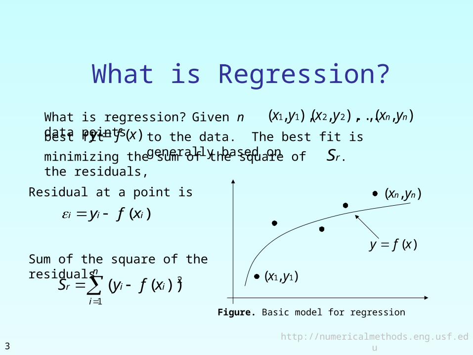
best fit )(xfy to the data. The best fit is generally based onminimizing the sum of the square of the
residuals, rS
Residual at a point is
)( iii xfy
n
i
iir xfyS1
2))((),( 11 yx
),( nn yx
)(xfy
Figure. Basic model for regression
Sum of the square of the residuals
.
http://numericalmethods.eng.usf.edu4
Linear Regression-Criterion#1
),( , ... ),,(),,( 2211 nn yxyx yx
Given n data points
best fit xaay 10
to the data.
Does minimizing
n
ii
1
work as a criterion, where )( 10 iii xaay
x
iiixaay
10
11, yx
22, yx
33, yx
nnyx ,
iiyx ,
iiixaay
10
y
Figure. Linear regression of y vs. x data showing residuals at a typical
point, xi .
http://numericalmethods.eng.usf.edu5
Example for Criterion#1
x y
2.0 4.0
3.0 6.0
2.0 6.0
3.0 8.0
Example: Given the data points (2,4), (3,6), (2,6) and (3,8), best fit the data to a straight line using Criterion#1
Figure. Data points for y vs. x data.
Table. Data Points
0
2
4
6
8
10
0 1 2 3 4
x
y
http://numericalmethods.eng.usf.edu6
Linear Regression-Criteria#1
04
1
i
i
x y ypredicted ε = y - ypredicted
2.0 4.0 4.0 0.0
3.0 6.0 8.0 -2.0
2.0 6.0 4.0 2.0
3.0 8.0 8.0 0.0
Table. Residuals at each point for regression model y = 4x – 4.
Figure. Regression curve for y=4x-4, y vs. x data
0
2
4
6
8
10
0 1 2 3 4
x
y
Using y=4x-4 as the regression curve
http://numericalmethods.eng.usf.edu7
Linear Regression-Criteria#1
x y ypredicted ε = y - ypredicted
2.0 4.0 6.0 -2.0
3.0 6.0 6.0 0.0
2.0 6.0 6.0 0.0
3.0 8.0 6.0 2.0
04
1
i
i
0
2
4
6
8
10
0 1 2 3 4
x
y
Table. Residuals at each point for y=6
Figure. Regression curve for y=6, y vs. x data
Using y=6 as a regression curve
http://numericalmethods.eng.usf.edu8
Linear Regression – Criterion #1
04
1
i
i for both regression models of y=4x-4 and y=6.
The sum of the residuals is as small as possible, that is zero, but the regression model is not unique.
Hence the above criterion of minimizing the sum of the residuals is a bad criterion.
http://numericalmethods.eng.usf.edu9
Linear Regression-Criterion#2
x
iiixaay
10
11, yx
22, yx
33, yx
nnyx ,
iiyx ,
iiixaay
10
y
Figure. Linear regression of y vs. x data showing residuals at a typical
point, xi .
Will minimizing
n
ii
1
work any better?
http://numericalmethods.eng.usf.edu10
Linear Regression-Criteria 2
x y ypredicted |ε| = |y - ypredicted|
2.0 4.0 4.0 0.0
3.0 6.0 8.0 2.0
2.0 6.0 4.0 2.0
3.0 8.0 8.0 0.0
0
2
4
6
8
10
0 1 2 3 4
x
y
Table. The absolute residuals employing the y=4x-4 regression model
Figure. Regression curve for y=4x-4, y vs. x data
44
1
i
i
Using y=4x-4 as the regression curve
http://numericalmethods.eng.usf.edu11
Linear Regression-Criteria#2
x y ypredicted |ε| = |y – ypredicted|
2.0 4.0 6.0 2.0
3.0 6.0 6.0 0.0
2.0 6.0 6.0 0.0
3.0 8.0 6.0 2.0
44
1
i
i
Table. Absolute residuals employing the y=6 model
0
2
4
6
8
10
0 1 2 3 4
x
y
Figure. Regression curve for y=6, y vs. x data
Using y=6 as a regression curve
http://numericalmethods.eng.usf.edu12
Linear Regression-Criterion#2
Can you find a regression line for which
44
1
i
i
for both regression models of y=4x-4 and y=6.
The sum of the absolute residuals has been made as small as possible, that is 4, but the regression model is not unique.
Hence the above criterion of minimizing the sum of the absolute value of the residuals is also a bad criterion.
44
1
i
i
http://numericalmethods.eng.usf.edu13
Least Squares Criterion
The least squares criterion minimizes the sum of the square of the residuals in the model, and also produces a unique line.
2
110
1
2
n
iii
n
iir xaayS
x
iiixaay
10
11, yx
22, yx
33, yx
nnyx ,
iiyx ,
iiixaay
10
y
Figure. Linear regression of y vs. x data showing residuals at a typical
point, xi .
http://numericalmethods.eng.usf.edu14
Finding Constants of Linear Model
2
110
1
2
n
iii
n
iir xaayS Minimize the sum of the square of the
residuals:To find
0121
100
n
iii
r xaaya
S
021
101
n
iiii
r xxaaya
S
giving
i
n
iii
n
ii
n
i
xyxaxa
1
2
11
10
0a and
1a we minimize
with respect to
1a 0aand
rS .
n
iii
n
i
n
i
yxaa11
11
0
http://numericalmethods.eng.usf.edu15
Finding Constants of Linear Model
0a
Solving for
2
11
2
1111
n
ii
n
ii
n
ii
n
ii
n
iii
xxn
yxyxn
a
and
2
11
2
1111
2
0
n
ii
n
ii
n
iii
n
ii
n
ii
n
ii
xxn
yxxyx
a
1aand directly yields,
xaya 10
http://numericalmethods.eng.usf.edu16
Example 1
The torque, T needed to turn the torsion spring of a mousetrap through an angle, is given below.
Angle, θ Torque, T
Radians N-m
0.698132 0.188224
0.959931 0.209138
1.134464 0.230052
1.570796 0.250965
1.919862 0.313707
Table: Torque vs Angle for a torsional spring
Find the constants for the model given by21 kkT
Figure. Data points for Torque vs Angle data
0.1
0.2
0.3
0.4
0.5 1 1.5 2
θ (radians)
To
rqu
e (
N-m
)
http://numericalmethods.eng.usf.edu17
Example 1 cont.
1a
The following table shows the summations needed for the calculations of the constants in the regression model.
2 T
Radians N-m Radians2 N-m-Radians
0.698132 0.188224 0.487388 0.131405
0.959931 0.209138 0.921468 0.200758
1.134464 0.230052 1.2870 0.260986
1.570796 0.250965 2.4674 0.394215
1.919862 0.313707 3.6859 0.602274
6.2831 1.1921 8.8491 1.5896
Table. Tabulation of data for calculation of important
5
1i
5nUsing equations described for
25
1
5
1
2
5
1
5
1
5
12
ii
ii
ii
ii
iii
n
TTnk
228316849185
1921128316589615
..
...
21060919 . N-m/rad
summations
0aTand
with
http://numericalmethods.eng.usf.edu18
Example 1 cont.
n
TT i
i
5
1_
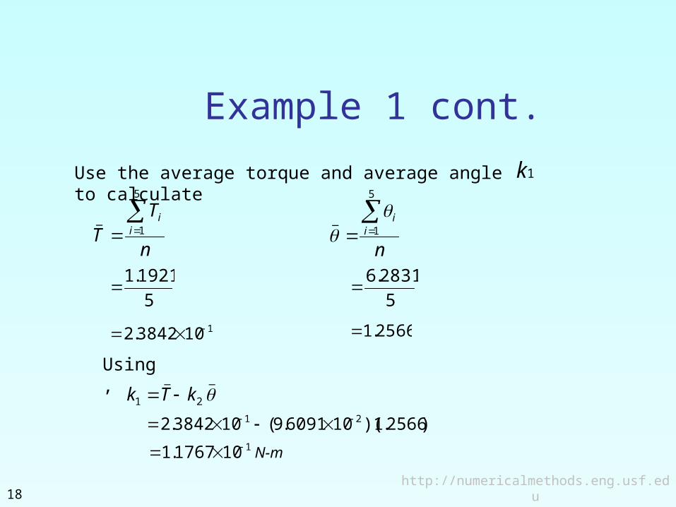
Use the average torque and average angle to calculate
1k
_
2
_
1 kTk
ni
i
5
1_
5
1921.1
1103842.2
5
2831.6
2566.1
Using,
)2566.1)(106091.9(103842.2 21 1101767.1 N-m
http://numericalmethods.eng.usf.edu19
Example 1 Results
Figure. Linear regression of Torque versus Angle data
Using linear regression, a trend line is found from the data
Can you find the energy in the spring if it is twisted from 0 to 180 degrees?
http://numericalmethods.eng.usf.edu20
Linear Regression (special case)
Given
best fit
to the data.
),( , ... ),,(),,( 2211 nn yxyx yx
xay 1
http://numericalmethods.eng.usf.edu21
Linear Regression (special case cont.)
Is this correct?
2
11
2
1111
n
ii
n
ii
n
ii
n
ii
n
iii
xxn
yxyxn
a
xay 1
http://numericalmethods.eng.usf.edu22
x
11, yx
ii xax 1,
nnyx ,
iiyx ,
iii xay 1
y
Linear Regression (special case cont.)
http://numericalmethods.eng.usf.edu23
Linear Regression (special case cont.)
iii xay 1
n
iirS
1
2
2
11
n
iii xay
Residual at each data point
Sum of square of residuals
http://numericalmethods.eng.usf.edu24
Linear Regression (special case cont.)
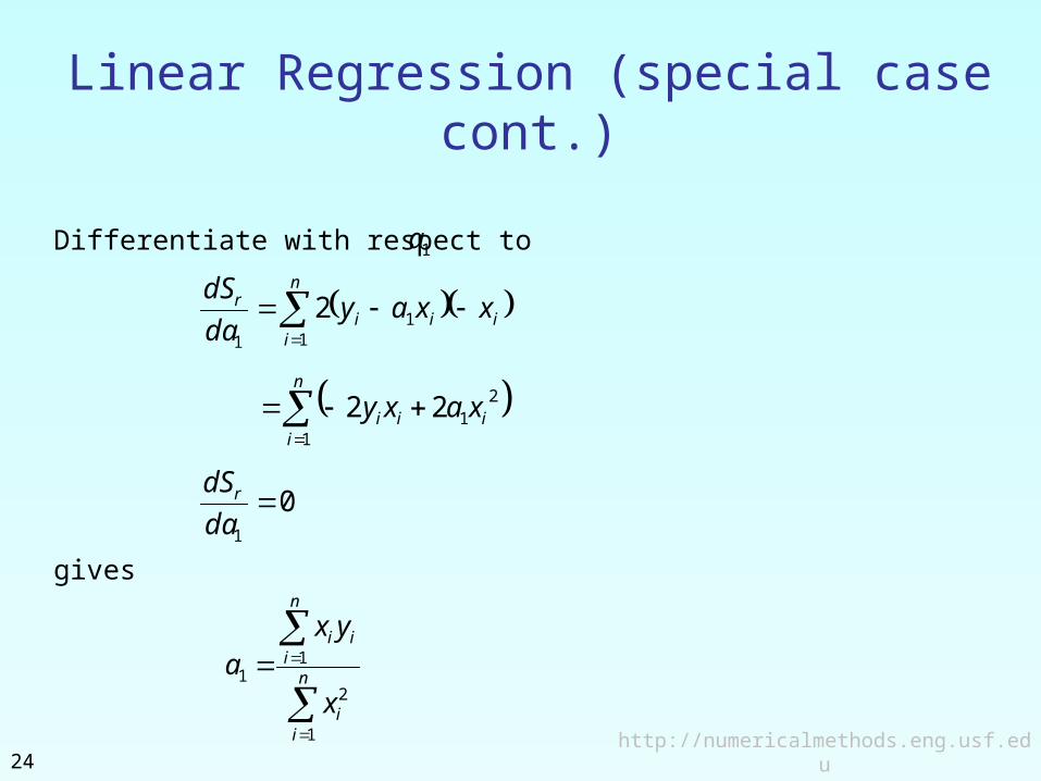
Differentiate with respect to
gives
n
iiii
r xxayda
dS
11
1
2
n
iiii xaxy
1
2122
01
da
dS r
n
ii
n
iii
x
yxa
1
2
11
1a
http://numericalmethods.eng.usf.edu25
Linear Regression (special case cont.)
n
ii
n
iii
x
yxa
1
2
11
n
iiii
r xaxyda
dS
1
21
1
22
021
2
21
2
n
ii
r xda
Sd
n
ii
n
iii
x
yxa
1
2
11
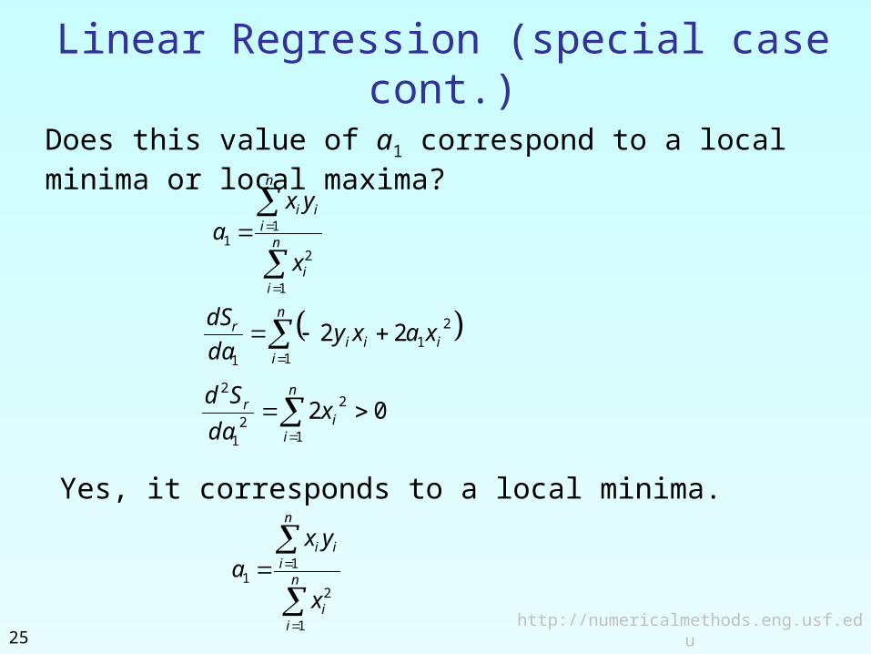
Does this value of a1 correspond to a local minima or local maxima?
Yes, it corresponds to a local minima.
http://numericalmethods.eng.usf.edu26
Linear Regression (special case cont.)
Is this local minima of an absolute minimum of ?
rS rS
1a
rS
http://numericalmethods.eng.usf.edu27
Example 2
Strain Stress
(%) (MPa)
0 0
0.183 306
0.36 612
0.5324 917
0.702 1223
0.867 1529
1.0244 1835
1.1774 2140
1.329 2446
1.479 2752
1.5 2767
1.56 2896
To find the longitudinal modulus of composite, the following data is collected. Find the longitudinal modulus, Table. Stress vs. Strain data
E using the regression model E and the sum of the square of
the
0.0E+00
1.0E+09
2.0E+09
3.0E+09
0 0.005 0.01 0.015 0.02
Strain, ε (m/m)
Str
ess,
σ (
Pa)
residuals.
Figure. Data points for Stress vs. Strain data
http://numericalmethods.eng.usf.edu28
Example 2 cont.
i ε σ ε 2 εσ
1 0.0000 0.0000 0.0000 0.0000
2 1.8300×10⁻³ 3.0600×10⁸ 3.3489×10⁻⁶ 5.5998×10⁵
3 3.6000×10⁻³ 6.1200×10⁸ 1.2960×10⁻⁵ 2.2032×10⁶
4 5.3240×10⁻³ 9.1700×10⁸ 2.8345×10⁻⁵ 4.8821×10⁶
5 7.0200×10⁻³ 1.2230×10⁹ 4.9280×10⁻⁵ 8.5855×10⁶
6 8.6700×10⁻³ 1.5290×10⁹ 7.5169×10⁻⁵ 1.3256×10⁷
7 1.0244×10⁻² 1.8350×10⁹ 1.0494×10⁻⁴ 1.8798×10⁷
8 1.1774×10⁻² 2.1400×10⁹ 1.3863×10⁻⁴ 2.5196×10⁷
9 1.3290×10⁻² 2.4460×10⁹ 1.7662×10⁻⁴ 3.2507×10⁷
10 1.4790×10⁻² 2.7520×10⁹ 2.1874×10⁻⁴ 4.0702×10⁷
11 1.5000×10⁻² 2.7670×10⁹ 2.2500×10⁻⁴ 4.1505×10⁷
12 1.5600×10⁻² 2.8960×10⁹ 2.4336×10⁻⁴ 4.5178×10⁷
1.2764×10⁻³ 2.3337×10⁸
Table. Summation data for regression model
12
1i
12
1
32 102764.1i
i
12
1
8103337.2i
ii
12
1
2
12
1
ii
iii
E
3
8
102764.1
103337.2
GPa84.182
n
ii
n
iii
E
1
2
1
http://numericalmethods.eng.usf.edu29
Example 2 Results 91084.182 The
equation
Figure. Linear regression for stress vs. strain data
describes the data.
Additional ResourcesFor all resources on this topic such as digital audiovisual lectures, primers, textbook chapters, multiple-choice tests, worksheets in MATLAB, MATHEMATICA, MathCad and MAPLE, blogs, related physical problems, please visit