www.tecnun.es Linear systems of ordinary differential equations (This is a draft and preliminary version of the lectures given by Prof. Colin Atkinson FRS on 21st, 22nd and 25th April 2008 at Tecnun) Introduction. This chapter studies the solution of a system of ordinary differential equations. These kind of problems appear in many physical or chemical models where sev- eral variables depend upon the same independent one. For instance, Newton’s second law applied to a particle. m · d 2 x 1 dt 2 = F 1 (x 1 ,x 2 ,x 3 , ˙ x 1 , ˙ x 2 , ˙ x 3 ,t) m · d 2 x 2 dt 2 = F 2 (x 1 ,x 2 ,x 3 , ˙ x 1 , ˙ x 2 , ˙ x 3 ,t) m · d 2 x 3 dt 2 = F 3 (x 1 ,x 2 ,x 3 , ˙ x 1 , ˙ x 2 , ˙ x 3 ,t) (1) Let us consider this system of ordinary differential equations: dx dt = -3x +3y dy dt = -xz + rx - y dx dt = xy - z (2) where x, y, z are time-dependent variables, and r is a parameter. We find a system of three non-linear ODE’s. The interesting thing in this example is the strong dependence of the solution on the paramater r and the initial value conditions (t 0 ,x 0 ,y 0 ,z 0 ). For the above reasons, the system presents as the chaos theory; a very known theory in Mathematics knows as the ”butterfly effect” 1 . These equations were posed by Lorenz in the study of metheorology. 1 The phrase refers to the idea that a butterfly’s wings might create tiny changes in the atmosphere that may ultimately alter the path of a tornado or delay, accelerate or even prevent the occurrence of a tornado in a certain location. The flapping wing represents a small change in the initial condition of the system, which causes a chain of events leading to large-scale alterations of events. Had the butterfly not flapped its wings, the trajectory of the system might have been vastly different. While the butterfly does not cause the tornado, the flap of its wings is an essential part of the initial conditions resulting in a tornado. Recurrence, the approximate return of a system towards its initial conditions, together with sensitive dependence on initial conditions are the two main ingredients for chaotic motion. They have the practical consequence of making complex systems, such as the weather, difficult to predict past a certain time range (approximately a week in the case of weather). c 2008 Tecnun (University of Navarra) 1
Transcript
www.tecn
un.es
Linear systems of ordinary differential equations
(This is a draft and preliminary version of the lectures given by Prof. ColinAtkinson FRS on 21st, 22nd and 25th April 2008 at Tecnun)
Introduction.
This chapter studies the solution of a system of ordinary differential equations.These kind of problems appear in many physical or chemical models where sev-eral variables depend upon the same independent one. For instance, Newton’ssecond law applied to a particle.
m · d2x1
dt2= F1(x1, x2, x3, x1, x2, x3, t)
m · d2x2
dt2= F2(x1, x2, x3, x1, x2, x3, t)
m · d2x3
dt2= F3(x1, x2, x3, x1, x2, x3, t)
(1)
Let us consider this system of ordinary differential equations:
dx
dt= −3x+ 3y
dy
dt= −xz + rx− y
dx
dt= xy − z
(2)
where x, y, z are time-dependent variables, and r is a parameter. We finda system of three non-linear ODE’s. The interesting thing in this example isthe strong dependence of the solution on the paramater r and the initial valueconditions (t0, x0, y0, z0). For the above reasons, the system presents as thechaos theory; a very known theory in Mathematics knows as the ”butterflyeffect”1. These equations were posed by Lorenz in the study of metheorology.
1The phrase refers to the idea that a butterfly’s wings might create tiny changes in theatmosphere that may ultimately alter the path of a tornado or delay, accelerate or even preventthe occurrence of a tornado in a certain location. The flapping wing represents a small changein the initial condition of the system, which causes a chain of events leading to large-scalealterations of events. Had the butterfly not flapped its wings, the trajectory of the systemmight have been vastly different. While the butterfly does not cause the tornado, the flapof its wings is an essential part of the initial conditions resulting in a tornado. Recurrence,the approximate return of a system towards its initial conditions, together with sensitivedependence on initial conditions are the two main ingredients for chaotic motion. They havethe practical consequence of making complex systems, such as the weather, difficult to predictpast a certain time range (approximately a week in the case of weather).
There is an important relationship between the system of ODE and the ODE’sof any order superior to the first. It is a matter of fact, that an equation oforder nth
y(n) = F (t, y, y′, y′′, . . . , y(n−1)) (3)
where y(n) = dny/dtn. This can be converted in a system of n equations of firstorder. With this change of variables
we reach n non-linear ODE’s of first order.There are three questions to be answered:(1) What about the existence of solutions?(2) What about uniqueness?(3) What is the sensitivity to the initial conditions?We are going to see in which cases we can assert that a system of ODE has asolution and this is unique. We must consider the following theoremTheorem. Let us assume that in a region A of the space (t, x1, x2, . . . , xn), thefunctions F1, F2, . . . , Fn and
∂F1
∂x1,∂F1
∂x2, . . . ,
∂F1
∂xn
∂F2
∂x1,∂F2
∂x2, . . . ,
∂F2
∂xn. . .∂Fn∂x1
,∂Fn∂x2
, . . . ,∂Fn∂xn
(6)
are continuous and such that the point (t0, x01, x
02, . . . , x
0n) is an interior point of
A. Thus there exists an interval
|t− t0| < ε (7)
(local argument) where there is a unique solution of the system given by eq. 5,
A way to prove this theorem is to use the Taylor’s expansion of the functions.Note.- We must point out that this is a sufficient condition theorem. So, weak-ening the conditions we can define a stronger expression of this theorem to geta unique solution.The systems are classified in the same manner as the ODE’s. They are linearand non-linear. If the functions F1, F2, . . . , Fn can be written as
with i = 1, 2, . . . , n, the system is called linear. If qi(t) are equal to zero forall i, this system is called linear and homogeneous; if not, non-homogeneous.For this kind of systems the theorem of existence and uniqueness is simpler andto some extent, more satisfactory. This theorem has global character. Noticethat in the general case this theorem it is defined in the neighbourhood of theinitial conditions, consequently giving a local character to the existence anduniqueness of the solution.Recall: If an equation is linear, it means we can add solutions together and stillsatisfy the differential equation, e.g. x′1 = H(x1) and H is linear, then
If q(t) = 0, we have an homogeneous system and eq. 14 becomes
x′ = P(t) · x (16)
This notation emphasises the relationship between the linear systems of ODE’sand the first order linear differential equationsTheorem. If x1 and x2 are solutions of eq. 16, so (c1 · x1 + c2 · x2) is solutionas well.
The question to be answered is: how many independent solutions of eq. 16are there? Let us assume at the moment, if x1,x2, . . . ,xn are solutions of thesystem, consider the matrix Ψ(t) –called fundamental matrix– given by
This is the Abel’s formula. Solving the differential equation
W (t) = W (t0) · e∫ t
t0(trace P(s))·ds (27)
As ex is never zero, W (t) 6= 0 for all finite value of t if trace P(t) is integrableand W (t0) 6= 0.
In n-dimensions the same happens. This generalises to n-dimensions to give
dW
dt= (P11 + · · ·+ Pnn) ·W (t) ⇒ W (t) = W (t0) · e
∫ tt0
(trace P(s))·ds
Example 2. A Sturm-Liouville equation has the form
d
dt
(a(t) · dy
dt
)+ b(t) · y = 0 (28)
This is a second order differential equation of the form
a2(t) · d2y
dt2+ a1(t) · dy
dt+ a0(t) · y = 0
This kind of equations were studied in 18th/19th century and early 20th century,where a2(t), a1(t) and a0(t) are linear in t. For instance, the vibration of a plateis given by these equations. We now write eq. (28) as a system
x1 = y (29)
x2 =dy
dt(30)
Then it gives
x′1 = x2 (31)
x′2 = −a′(t)a(t)
· x2 −b(t)a(t)
· x1 (32)
We could use our theory of systems to get the connection –wronskian– betweenx1 and x2 independent solutions of the system. However, we consider eq. (28)directly assuming that y1 and y2 are two possible solutions. So
Homogeneous linear system with constant coefficients.
Let us consider the systemx′ = A · x (37)
where A is real , n× n constant matrix. As solution, we will try
x = er·t · a (38)
where a is a constant vector. Then
x′ = r · er·t · a (39)
Then we have a solution provided that
r · er·t · a = A · er·t · a ⇔ (A− r · I) · a = 0 (40)
and for non-trivial solution (i.e. a 6= 0), r must satisfy
|A− r · I| = 0 (41)
Procedure.
Finding eigenvalues, r1, r2, . . . , rn, solution of |A− r · I| = 0 and correspondingeigenvectors, a1,a2, . . . ,an. Then if the n eigenvectors are linearly independent,we have a general solution
where c1, c2, . . . , cn are arbitrary constants. Recall ai = (a1i a2i . . . ani) andxi = ai · eri·t, with i = 1, 2, . . . , n. Then the wronskian will be
W (t) =
∣∣∣∣∣∣∣∣∣a11 a12 . . . a1n
a21 a22 . . . a2n
......
. . ....
an1 an2 . . . ann
∣∣∣∣∣∣∣∣∣ e(r1+r2+···+rn)·t 6= 0 (43)
since a1,a2, . . . ,an are linearly independent. In a large number of problems,getting the eigenvalues can be very difficult problem.
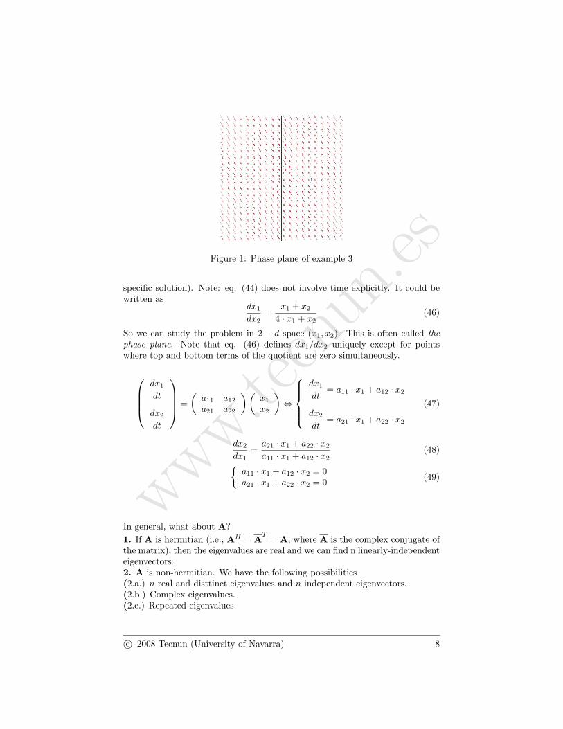
Example 3.
x′ =(
1 14 1
)· x (44)
Consider x = a · er·t. Then we require
(A− r · I) ·(a11
a21
)=(
00
)
|A− r · I| =∣∣∣∣1− r 1
4 1− r
∣∣∣∣ = 0
(1− r)2 − 4 = 0 ⇒ (1− r)2 = 4 ⇒ 1− r = ±2
r = 3, −1. So the eigenvalues are 3 and −1. With r = 3(−2 14 −2
)·(a1
a2
)=(
00
)So −2 · a1 + a2 = 0 implies that a1 = 1 and a2 = 2. Hence, the eigenvector willbe (
12
)With r = −1 (
2 14 2
)·(a1
a2
)=(
00
)So 2 · a1 + a2 = 0 implies that a1 = 1 and a2 = −2. Therefore, the eigenvectorwill be (
1−2
)The general solution is
x = C1 ·(
12
)· e3·t + C2 ·
(1−2
)· e−t (45)
The equation (45) is a family of solutions since C1 and C2 are arbitrary (i.e.,if x1 and x2 are known at t = 0, we can solve eq. (45) to get C1 and C2 for
specific solution). Note: eq. (44) does not involve time explicitly. It could bewritten as
dx1
dx2=
x1 + x2
4 · x1 + x2(46)
So we can study the problem in 2 − d space (x1, x2). This is often called thephase plane. Note that eq. (46) defines dx1/dx2 uniquely except for pointswhere top and bottom terms of the quotient are zero simultaneously.
In general, what about A?1. If A is hermitian (i.e., AH = A
T= A, where A is the complex conjugate of
the matrix), then the eigenvalues are real and we can find n linearly-independenteigenvectors.2. A is non-hermitian. We have the following possibilities(2.a.) n real and disttinct eigenvalues and n independent eigenvectors.(2.b.) Complex eigenvalues.(2.c.) Repeated eigenvalues.
we obtain r1 = −1 y r2 = 3. We need the eigenvectors
r1 = −1⇒ a1 = (1 − 2)T
r2 = 3⇒ a2 = (1 2)T (52)
We have two solutions
x1 =(
1−2
)e−t x2 =
(12
)e3t (53)
To find the general solution, we construct it via a linear combination –by addingthese two linearly independent solutions together–
x = c1 · e−t ·(
1−2
)+ c2 · e3·t ·
(12
)(54)
c1 and c2 are arbitrary constants to be determined by intial conditions or otherconditions on x.
We can plot (see Figure 2) the family of the solutions in the (x1, x2) plane withan arrow to signify the direction of time (means time increasing). Our solutionin components looks like
x1 =c1 · e3·t + c2 · e−t
x2 =2 · c1 · e3·t − 2 · c2 · e−t
we can study the motion of a pendulum, we can use systems in order to studyposition and velocity. Suppose c2 ≡ 0 and we are interested in the point x1 =x2 = 0 and note x1/x2 = 1/2 with c1 6= 0. We only reach (0, 0) if t→ −∞ sincewe need e3·t → 0. If c1 ≡ 0 and c2 6= 0, then x1/x2 = −1/2. To get (0, 0) weneed t→ +∞. So (0, 0) is a special point. I can represent the time by an arrow
t→ −∞⇒{x1 → c1 · e−tx2 → −2 · c1 · e−t
⇔ x2 → −2 · x1
t→ +∞⇒{x1 → c2 · e3·tx2 → 2 · c2 · e3·t
⇔ x2 → 2 · x1
(55)
Point (0, 0) is a saddle point. Thinking of the future, we can observe thatdetA = −3 < 0.
We are looking for real solution to this system. We know that a linear combi-nation of these solutions will be a solution as well. Hence, we can take the realand the imaginary parts of these ones
Plotting this family of curves on the phase plane (x1, x2)
Figure 4: Phase plane of Example 7
t→ +∞⇒{x1 → 0x2 → 0 ⇔ (x1, x2)→ (0, 0) (79)
Let us study the points (x 0)T y (0 y)T . Substituting into eq. 73
x = (x 0)T ⇒ x′ = (−x/2 − x)T ⇒ dy
dx= 2
x = (0 y)T ⇒ x′ = (y − y/2)T ⇒ dy
dx=−12
(80)
Point (0, 0) is a stable spiral point. Thinking of the future once again, det A =5/4 > 0, traceA = −1 < 0 and detA > (traceA)2/4.
Repeated eigenvalues.
Let us consider the system given by eq. 37, with A a real non-symmetric matrix.Let us assume that one of its eigenvalues, r1, is repeated (m1 = m > 1), andthere are not m linearly independent eigenvectors, 1 ≤ k < m. We shouldobtain (m − k) additional linearly independent solutions. How do we amendthe procedure to deal with cases when there are no m linearly independenteigenvectors?For example, the exponential of a square matrix:
We recall the Cayley–Hamilton theorem. If f(λ) is the characteristic poynomialof a matrix A,
f(λ) = det (A− λ · I) (82)
This theorem says that f(A) = 0. For instance,
f(λ) = r2i − (trace ·A)ri + det A = r2i − p · ri + q = 0 (83)
Hence, by Cayley-Hamilton theorem,
f(A) = A2 − p ·A + q · I = 0 (84)
using this theorem, any expansion function like eA can be reduced to polynomi-als on A. This is very useful theorem in problems of materials and continuummechanics.
A2 = p ·A− q·IA3 = p ·A2 − q ·A =
(p2 − q
)·A− p · q · I
A4 = p ·A3 − q ·A2 = p ·(p2 − 2q
)·A− (p2 − q) · q · I
. . .
(85)
So, we can use this theorem to get a finite expansion of eq. 81.Differentiating with respect to t that expression
But x = eA·t ·v is a solution of the system. Moreover, let us assume that v = ai
where ai is an eigenvector of ri, then
x = eri·t(
I + t(A− ri · I) +t2
2!(A− ri · I)2 + . . .
)· ai =
= eri·t(
ai + t · (A− ri · I) · ai +t2
2!· (A− ri · I)2 · ai + . . .
)=
(96)
But, as ai is eigenvector, it verifies
(A− ri · I) · ai = 0 = (A− ri · I)2 · ai = (A− ri · I)3 · ai = . . . (97)
Then eq. 96 becomesx = eri·t · ai (98)
We can look for another vector v such that
(A− ri · I) · v 6= 0 y (A− ri · I)2 · v = 0 = (A− ri · I)3 · v = . . . (99)
Lemma. Let us assume that the characteristic polynomial of A, non-hermitian,of order n, have repeated roots (r1, r2, . . . , rk, 1 ≤ k < n), of order (m1,m2, . . . ,mk
(m1 +m2 + · · ·+mk = n), respectively such that
f(λ) = (λ− r1)m1(λ− r2)m2 . . . (λ− rk)mk (100)
if A has only nj < mj eigenvectors of the eigenvalue rj (i.e., (A− rj · I) · v = 0has nj independent solutions), then (A − rj · I)2 · v = 0 has at least nj + 1independent solutions. In general, if (A − rj · I)m · v = 0 has got nj < mj
independent solutions, (A − rj · I)m+1 · v = 0 has at least nj + 1 independentsolutions
As (A − r1I)2 = (A − r1I)3 = 0, any vector a2 verifies eq. 106. However,according to the inequality given by eq. 105, a2 cannot be a linearly dependentvector of a1 (eq. 103). So
a2 = (0 1)T ⇒(
0 10 0
)·(
01
)=(
10
)6= 0 (107)
From eq. 96, we obtain
x2 = et ·(
a2 + t · (A− r1 · I) · a2 +t2
2!· (A− r1 · I)2 · a2 + . . .
)=
= et ·((
01
)+ t
(10
)+ 0)
= et ·(
t1
) (108)
The general solution is
x = c1 · et ·(
10
)+ c2 · et ·
(t1
)(109)
Thinking of next paragraph, detA = 1 > 0, traceA = 2 > 0 and detA =(traceA)2/4.
Resume of the study of a system of two homogeneous equations withconstant coefficients.
Let us consider the system
x′ = a · x+ b · yy′ = c · x+ d · y (110)
its characteristic polynomial is
f(r) = r2 − p · r + q (111)
where p = a+ d (the trace) y q = a · d− b · c (the determinant). Its eigenvaluesare
r =p±
√p2 − 4 · q2
(112)
The study of eigenvalues and eigenvectors is very useful in order to classifythe critical point (0, 0) and to know the trajectories on the phase plane.
1. q < 0. The eigenvalues are positive and negative, respectively. Saddle point.
2. q > 0.2.a. p2 > 4q. Both eigenvalues are either positive or negative.- Stable node, if p < 0.- Unstable node, if p > 0.2.b. p2 < 4 · q. The eigenvalues are complex conjugates.- Stable spiral, if p < 0.- Unstable spiral, if p > 0.- Center, if p = 0.2.c. p2 = 4 · q. The eigenvalue is a double root of the characteristic polynomial.- Stable node, if p < 0 and there is only one eigenvector.- Unstable node, if p > 0 and there is only one eigenvector.
- Sink point, if p < 0 and there are two independent eigenvectors.- Source point, if p > 0 and there are two independent eigenvectors.3. q = 0. It means that the matrix rank is 1 and therefore, one row can beobtained multipliying the other one by a constant (c/a = d/b = k). Then, (0, 0)is not an isolated critical point. There is a line y = −a · x/b, b 6= 0, of criticalpoints. The trajectories on the phase plane are y = k ·x+E, E being a constant.- If p > 0, paths start at the critical points and go to the infinity.- If p < 0, conversely, the trajectories end at the critical points.
It is very convenient and useful to know the plane trace-determinant (p, q).
Fundamental matrix of a system
Let us consider the homogeneos system given by eq. 16 and let x1,x2, . . . ,xn
be a set of its independent solutions. We know that we can build the generalsolution via a linear combination of them. We denote fundamental matrix, Ψ(t),a matrix whose columns are the solution vectors of eq. 18. The determinant ofthis matrix is not zero (eq. 19). This determinant is called wronskian (eq. 20).Let us assume that we are looking for a solution x such that x(t0) = x0. Then
where c = (c1 c2 . . . cn)T . As |Ψ(t)| 6= 0,∀t, c can be obtained using theinverse matrix of Ψ(t0):
c = Ψ−1(t0) · x0 (114)and the solution will be
x = Ψ(t) ·Ψ−1(t0) · x0 (115)
This matrix is very useful when
Ψ(t0) = I (116)
This special set of solutions builds the matrix Φ(t). It verifies
x = Φ(t) · x0 (117)
We obtain that Φ(t) = Ψ(t) ·Ψ−1(t0).Moreover, with constant coefficients:
(1.) eA·t (eq. 81) is a fundamental matrix of fundamental solutions since itverifies eq. 86 and eA·0 = I.(2.) If we know two fundamental matrices of the system, Ψ1 and Ψ2, there isalways a constant matrix C such that Ψ2 = Ψ1 ·C, since each column of Ψ2
can be obtained by a linear combination of the columns of Ψ1.(3.) It can be shown that eA·t = Ψ(t) ·Ψ−1(t0) (see eq. 115). According toparagraphs 1 and 2, there exists a matrix C such that
We assume that we have solved x′ = P(t) ·x. We actually have a procedure forP(t) = A, a constant matrix.Consider special cases
(1)
If P(t) = A and A has n independent eigenvectors, the procedure is to buildthe matrix T with the eigenvectors of A:
T = (a1 a2 . . . an) (121)
Then, we change variables x = T ·y with x′ = T ·y′. Going back to the system
x′ = T · y′ = A · x + q = A ·T · y + q (122)
As T is built with n eigenvectors, this is a regular matrix (det T 6= 0), so wecan work out T−1, the inverse of T. Hence, from eq. 114
y′ = T−1 ·A ·T · y + T−1 · q = D · y + h (123)
where D is the diagonal matrix of the eigenvalues of A. Therefore,
y′i(t) = ri · yi(t) + hi(t),∀i = 1, 2, . . . , n (124)
Henceyi(t) = erit ·
∫e−ri·t · hi(t) · dt+ ci · eri·t,∀i = 1, 2, . . . , n (125)
After obtaining yi, we can get x = T · y.This method is only possible if there are n linearly independent eigenvectors,
i.e., A is a diagonalizable constant matrix. Because we can reduce the matrixto its diagonal form, the above procedure works. In cases where we do not havethe n independent eigenvectors, the matrix A can only be reduced to its Jordancanonical form.
(2) Variation of the parameters.
Let us consider the system of eq. 14, and we know the solution of the associatedhomogeneous system (eq. 16). Then we can build the fundamental matrix ofthe system, Ψ(t) (eq. 18), whose columns are the linearly independent of thehomogeneous system solutions. We are looking for a solution like