Ordinary Di erential Equations. Week 6

Mechanical and Electrical Vibrations

Ordinary Differential Equations. Week 6

Dr. Marco A Roque Sol

02/20/2018

Dr. Marco A Roque Sol Ordinary Differential Equations. Week 6


Mechanical VibrationsForced VibrationsElectric VibrationsReduction of Order

Mechanical Vibrations


Second order linear equations with constant coefficients areimportant in two physical processes, namely, Mechanical andElectrical oscillations.

Actually from the Math point of view, both problems are the same.However, from the Physics point of view they are quite different.

For example, the motion of a mass on a vibrating spring, theangular motion of a simple pendulum, the flow of electric currentin a simple series circuit and the electrical charge in an electriccircuit, are just examples of that difference.





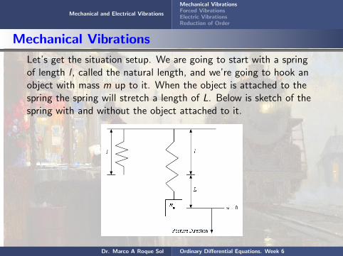
Let’s get the situation setup. We are going to start with a springof length l , called the natural length, and we’re going to hook anobject with mass m up to it. When the object is attached to thespring the spring will stretch a length of L. Below is sketch of thespring with and without the object attached to it.





Convention

As denoted in the sketch we are going to assume that all forces,velocities, and displacements in the downward direction will bepositive. All forces, velocities, and displacements in the upwarddirection will be negative.

Also, as shown in the sketch above, we will measure alldisplacement of the mass from its equilibrium position. Therefore,the u = 0 position will correspond to the center of gravity for themass as it hangs on the spring and is at rest.





Now, we need to develop a differential equation that will give thedisplacement of the object at any time t. First, recall Newton’sSecond Law of Motion.

F = ma

In this case we will use the second derivative of the displacement,u, for the acceleration and so Newton’s Second Law becomes,

F (t, u, u′) = mu′′

Here is a list of the forces that will act upon the object.





Gravity, Fg

The force due to gravity will always act upon the object of course.This force isMechanical and Electrical Vibrations

Fg = mgSpring, Fs

We are going to assume that Hookes Law will govern the forcethat the spring exerts on the object. This force will always bepresent as well and is

Fs = −k(L + u)

Hookes Law tells us that the force exerted by a spring will be thespring constant, k > 0, times the displacement of the spring fromits natural length.





Damping, Fd

The next force that we need to consider is damping. This forcemay or may not be present for any given problem. This force worksto counteract any movement. This damping force is

Fd = −γu′

where, γ > 0 is the damping coefficient.

External Forces, F (t)

If there are any other forces acting on our object we collect themin this term. We typically call F (t) the forcing function.





Putting all of these together gives us the following for NewtonsSecond Law.

mu′′ = mg − k(L + u)− γu′ + F (t)

Or, upon rewriting, we get,

mu′′ + γu′ + ku = mg − kL + F (t)

Now, when the object is at rest in its equilibrium position,

mg − kL = 0

Using this in Newtons Second Law gives us the final version of thedifferential equation that well work with.

mu′′ + γu′ + ku = F (t)Dr. Marco A Roque Sol Ordinary Differential Equations. Week 6




Along with this differential equation we will have the followinginitial conditions.

u(0) = u0 Initial displacement

u′(0) = u′0 Initial velocity

OBS

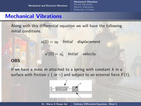
If we have a mass m attached to a spring with constant k in asurface with friction c ( or γ) and subject to an external force F (t),





then it satisfy the differential equation

mu′′ + cu′ + ku = F (t)

Free, Undamped Vibrations

This is the simplest case that we can consider. Free or unforcedvibrations means that F (t) = 0 and undamped vibrations meansthat γ = 0. In this case the differential equation becomes,

mu′′ + ku = 0

The characteristic equation has the roots,

r = ±√

k

m= ±ω0i ; ω0 =

√k

m





Where ω0 is called the natural frequency. Recall as well thatm > 0 and k > 0 and so we can guarantee that this quantity willnot be complex. The solution in this case is then

u(t) = c1cos(ω0t) + c2sin(ω0t)

We can write the above equation in the following form

u(t) = Rcos(ω0t − δ)

(If c1 = Rcos(δ) c2 = Rsin(δ) =⇒ u(t) = Rcos(δ)cos(ω0t)+Rsin(δ)sin(ω0t) =⇒ u(t) = Rcos(ω0t − δ); R2 = c21 + c22 ;tan(δ) = c2/c1

where R is the amplitude of the displacement and δ is the phaseshift or phase angle of the displacement. T = 2π

ω0= 2π

√mk is

called the natural period.Dr. Marco A Roque Sol Ordinary Differential Equations. Week 6




Example 55A 16 lb object stretches a spring 8/9 ft by itself. There is nodamping and no external forces acting on the system. The springis initially displaced 6 inches upwards from its equilibrium positionand given an initial velocity of 1 ft/sec downward. Find thedisplacement at any time t, u(t).

Solution

We first need to set up the IVP for the problem. We need to findm and k . This is the British system so we’ll need to compute themass.

m =W

g=

16

32=

1

2





Now, lets find k . We can use the fact that mg = kL to find k .We’ll use feet for the unit of measurement for this problem.

k =mg

L=

16

8/9= 18

We can now set up the IVP.

1

2u′′ + 18u = 0; u(0) = −1

2(6inches), u′(0) = 1

Now, the natural frequency, is

ω0 =

√18

1/2= 6





The general solution, along with its derivative, is then,

u(t) = c1cos(6t) + c2sin(6t)

u′(t) = −6c1sin(6t) + 6c2cos(6t)

Applying the initial conditions gives

−1

2= u(0) = c1 =⇒ c1 = −1

2

1 = u′(0) = 6c2 =⇒ c2 =1

6The displacement at any time t is then

u(t) = −1

2cos(6t) +

1

6sin(6t)





Now, lets convert this to a single cosine function. First let’s getthe amplitude, R.

R =

√(−1

2

)2

+

(1

6

)2

=

√10

6= 0.52705

Now let’s get the phase shift.

δ = tan−1(

1/6

−1/2

)= −0.32175

From the above equations, we have two angles

δ1 = −0.32175; δ2 = δ1 + π = 2.81984





We need to decide which of these phase shifts is correct, becauseonly one will be correct. To do this recall that

c1 = Rcos(δ) = −1/2 < 0; c2 = Rsin(δ) = 1/6 > 0

This means that the phase shift must be in Quadrant II and so thesecond angle is the one that we need. Thus, the displacement atany time t is.

u(t) =

√10

6cos(6t − δ); δ = tan−1

(−1

3

)+ π





Here is a sketch of the displacement for the first 5 seconds.





Free, Damped Vibrations

We are still going to assume that there will be no external forcesacting on the system, with the exception of damping of course. Inthis case the differential equation will be

mu′′ + γu′ + ku = 0

where m, γ, and k are all positive constants. Upon solving for theroots of the characteristic equation we get the following.

r1,2 =−γ ±

√γ2 − 4mk

2m





We will have three cases here.

1.− γ2 − 4mk = 0

In this case we will get a double root out of the characteristicequation and the displacement at any time t will be.

u(t) = c1e− γt

2m + c2te− γt

2m

Notice that as t →∞ the displacement will approach zero.

This case is called critical damping and will happen when thedamping coefficient is,

γ2 − 4mk = 0 =⇒ γ =√

4mk = γCR





The above value of the damping coefficient is called the criticaldamping coefficient and denoted by γCR .

2.− γ2 − 4mk > 0.

In this case let’s rewrite the roots

r1,2 =−γ ±

√γ2 − 4mk

2m= − γ

2m

(1±

√1− 4mk

γ2

)Also notice that from our initial assumption that we have,

4mk

γ2< 1 =⇒ 1− 4mk

γ2< 1 =⇒

√1− 4mk

γ2< 1





This means that the quantity in the parenthesis is guaranteed tobe positive and so the two roots in this case are guaranteed to benegative. Therefore the displacement at any time t is

u(t) = c1e− γ

2m

(1+√

1− 4mkγ2

)t

+ c2e− γ

2m

(1−√

1− 4mkγ2

)t

and will approach zero as t →∞.

This case will occur when

γ2 − 4mk > 0 =⇒ γ >√

4mk = γCR

and is called over damping.





3.− γ2 − 4mk < 0.

In this case we will get complex roots out of the characteristicequation.

r1,2 =−γ2m±√γ2 − 4mk

2m= λ± i µ

where the real part is guaranteed to be negative and so thedisplacement is

u(t) = e−γ2m

t

(c1cos(

√4mk − γ2

2mt) + c2sin(

√4mk − γ2

2mt)

)

u(t) = = Rcos(µt − δ)

Since λ < 0 the displacement will approach zero as t →∞ .Dr. Marco A Roque Sol Ordinary Differential Equations. Week 6




We will get this case will occur when

γ2 − 4mk < 0 =⇒ γ <√

4mk = γCR

and is called under damping.

Example 56

Take the spring and mass system from the example 55 and considerthere is a damping force to it that will exert a force of 17 lbs whenthe velocity is 2ft/s. Find the displacement at any time t, u(t).

Solution

So, the only difference between this example and the previousexample is damping force. So let’s find the damping coefficient

17 = γ(2) =⇒ γ = 2/17 = 8.5 > γCR =√

4km = 6





So it looks like we have got over damping this time around so weshould expect to get two real distinct roots from the characteristicequation and they should both be negative. The IVP for thisexample is

1

2u′′ +

17

2u′ + 18u = 0; u(0) = −1

2, u′(0) = 1

The roots of the characteristic equation are

r1,2 =−17±

√145

2

The general solution for this example is

u(t) = c1e−17+

√145

2t + c2e

−17−√

1452

t





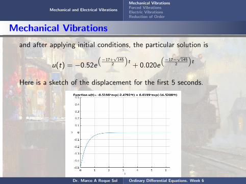
and after applying initial conditions, the particular solution is

u(t) = −0.52e

(−17+

√145

2

)t

+ 0.020e

(−17−

√145

2

)t

Here is a sketch of the displacement for the first 5 seconds.





Example 57

Take the spring and mass system from the example 55 and considerthere is a damping force to it that will exert a force of 12lbs whenthe velocity is 2ft/s. Find the displacement at any time t, u(t).

Solution

The damping coefficient is given by

12 = γ(2) =⇒ γ = 12/2 = 6 = γCR

So it looks like we have got critical damping this time. The IVPfor this problem is

1

2u′′ + 6u′ + 18u = 0; u(0) = −1

2, u′(0) = 1






r1,2 = − 6

(2)(1/2)= 6


u(t) = c1e−6t + c2te

−6t

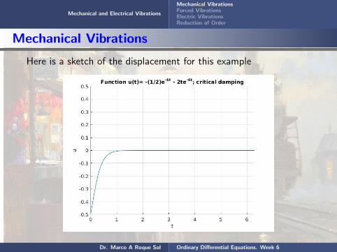
and after applying initial conditions, the particular solution is

u(t) = −1

2e−6t − 2te−6t





Here is a sketch of the displacement for this example





Example 58

Take the spring and mass system from the example 55 and considerthere is a damping force to it that will exert a force of 5lbs whenthe velocity is 2ft/s. Find the displacement at any time t, u(t).

Solution

The damping coefficient is given by

5 = γ(2) =⇒ γ = 5/2 = 2.5 < γCR

So it looks like we have got under damping this time. The IVP forthis problem is

1

2u′′ +

5

2u′ + 18u = 0; u(0) = −1

2, u′(0) = 1






r1,2 =−5±

√119 i

2


u(t) = e−52t

(c1cos

(√119

2t

)+ c2sin

(√119

2t

))and after applying initial conditions, the particular solution is

u(t) = e−5t2

(−0.5cos

(√119

2t

)− 0.046sin

(√119

2t

))





Lets convert this to a single cosine as we did in the undamped case.

R =√

(−0.5)2 + (.046)2 = 0.502 δ = tan−1 =

(−0.046

−0.5

)= 0.09

or δ = 0.09 + π = 3.23

This means δ must be in the Quadrant II ( why ?) and so thesecond angle is the one that we want. The displacement is then

u(t) = 0.502e−5t2 cos

(√119

2t − 3.23

)









Forced Vibrations

Undamped, Forced VibrationsWe will first take a look at the undamped case. The differentialequation in this case is

mu′′ + ku = F (t)

This is just a nonhomogeneous differential equation and we knowhow to solve these. The general solution will be

u(t) = uc + UP

There is a particular type of forcing function that we should take alook at since it leads to some interesting results. Lets suppose thatthe forcing function is a simple periodic function of the form

F (t) = F0cos(ωt) or F (t) = F0sin(ωt)




Forced Vibrations

For the purposes of this discussion we will use the first one. Usingthis, the ODE becomes,

mu′′ + ku = F0cos(ωt)

The solution of the associate homogeneous , as pointed out above,is just

uc(t) = c1cos(ω0t) + c2sin(ω0t)

where ω0 is the natural frequency.

We will need to be careful in finding a particular solution. Thereason for this will be clear if we use undetermined coefficients.With undetermined coefficients our guess for the form of theparticular solution would be,




Forced Vibrations

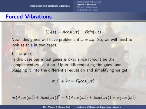
UP(t) = Acos(ωt) + Bsin(ωt)

Now, this guess will have problems if ω = ω0. So, we will need tolook at this in two cases.

1. ω 6= ω0

In this case our initial guess is okay since it wont be thecomplementary solution. Upon differentiating the guess andplugging it into the differential equation and simplifying we get,

mu′′ + ku = F0cos(ωt)

m (Acos(ωt) + Bsin(ωt))′′ + k (Acos(ωt) + Bsin(ωt)) = F0cos(ωt)




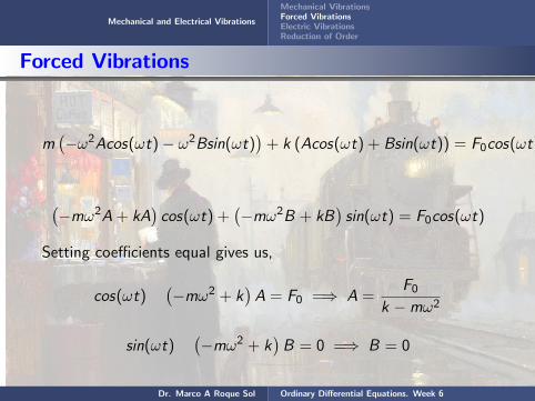
Forced Vibrations

m(−ω2Acos(ωt)− ω2Bsin(ωt)

)+ k (Acos(ωt) + Bsin(ωt)) = F0cos(ωt)

(−mω2A + kA

)cos(ωt) +

(−mω2B + kB

)sin(ωt) = F0cos(ωt)

Setting coefficients equal gives us,

cos(ωt)(−mω2 + k

)A = F0 =⇒ A =

F0k −mω2

sin(ωt)(−mω2 + k

)B = 0 =⇒ B = 0




Forced Vibrations

The particular solution is then

F0k −mω2

cos(ωt) =F0

m (k/m − ω2)cos(ωt) =

F0

m(ω20 − ω2

)cos(ωt)

Note that we rearranged things a little. Depending on the formthat you’d like the displacement to be in we can have either of thefollowing.

u(t) = c1cos(ω0t) + c2sin(ω0t) +F0

m(ω20 − ω2

)cos(ωt)

u(t) = Rcos(ω0t − δ) +F0

m(ω20 − ω2

)cos(ωt)

If we used the sine form of the forcing function we could get asimilar formula.




Forced Vibrations

2. ω = ω0

In this case we will need to add in a t to the guess for theparticular solution.

UP(t) = Atcos(ωt) + Btsin(ωt)

Differentiating our guess, plugging it into the differential equationand simplifying gives us the following.(

−mω20 + k

)Atcos(ωt) +

(−mω2

0 + k)Btsin(ω)t + ...

...+ 2mω0Bcos(ωt)− 2mω0Asin(ωt) = F0cos(ωt)

but (−mω2

0 + k)

= m(−ω2

0 + k/m)

= m(−ω2

0 + ω20

)= 0




Forced Vibrations

So, the first two terms actually drop out and this gives us

cos(ωt) 2mω0B = F0 =⇒ B =F0

2mω0

sin(ωt) 2mω0A = 0 =⇒ A = 0

In this case the particular will be,

F02mω0

tsin(ω0t)

The displacement for this case is then

u(t) = c1cos(ω0t) + c2sin(ω0t) +F0

2mω0tsin(ω0t)




Forced Vibrations

depending on the form that you prefer for the displacement.

u(t) = Rcos(ω0t − δ) +F0

2mω0tsin(ω0t)

So, what was the point of the two cases here? Well in the firstcase, our displacement function consists of two cosines and is niceand well behaved for all time.

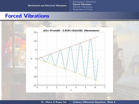
In contrast, the second case, will have some serious issues at tincreases. The addition of the t in the particular solution will meanthat we are going to see an oscillation that grows in amplitude as tincreases. This case is called resonance and we would generallylike to avoid this at all costs.




Forced Vibrations




Forced Vibrations

In this case resonance arose by assuming that the forcing functionwas,

F (t) = F0cos(ω0t)

We would also have the possibility of resonance if we assumed aforcing function of the form.

F (t) = F0sin(ω0t)

We should also take care to not assume that a forcing function willbe in one of these two forms. Forcing functions can come in a widevariety of forms. If we do run into a forcing function different fromthe one that used here you will have to go through undeterminedcoefficients or variation of parameters to determine the particularsolution.




Forced Vibrations

Example 59

A 3 kg object is attached to spring and will stretch the spring 392mm by itself. There is no damping in the system and a forcingfunction of the form

F (t) = 10cos(ωt)

is attached to the object and the system will experience resonance.If the object is initially displaced 20 cm downward from itsequilibrium position and given a velocity of 10 cm/sec upward findthe displacement at any time t.

Solution

Since we are in the metric system we wont need to find mass as itsbeen given to us. Also, for all calculations we will be converting alllengths over to meters. The first thing we need to do is find k.




Forced Vibrations

k =mg

L=

(3)(9.8)

0.392= 75

Now, we are told that the system experiences resonance so let’s goahead and get the natural frequency.

ω0 =

√k

m=

√75

3= 5

The IVP for this is then

3u′′ + 75u = 10cos(5t); u(0) = 0.2, u′(0) = −0.1

The complementary solution is the free undamped solution whichis easy to get and for the particular solution we can just use theformula that we derived above. The general solution is then,

u(t) = c1cos(5t) + c2sin(5t) +1

3tsin(5t)




Forced Vibrations

Applying the initial conditions gives

u(t) =1

5cos(5t)− 1

50sin(5t) +

1

3tsin(5t)

The last thing that we’ll do is combine the first two terms into asingle cosine.

R =

√(1

5

)2

+

(−1

50

)2

= 0.201 δ1 = tan−1(−1/50

1/5

)= −0.099

δ2 = δ1 + π = 3.042

In this case c1 > 0 is positive and c2 < 0 . This means that thephase shift needs to be in Quadrant IV and so the first one is thecorrect phase shift this time.




Forced Vibrations

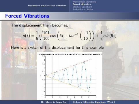
The displacement then becomes,

u(t) =1

5

√101

100cos

(5t + tan−1

(−1

10

))+

1

3tsin(5t)





Forced Vibrations

Example 60

Solve the initial value problem and plot the solution.

u′′ + u = 0.5cos(0.8t), u(0) = 0, u′(0) = 0

Solution

The general solution of is

u = c1cos(ω0t) + c2sin(ω0t) +F0

m(ω20 − ω2)

cos(ωt)

Applying initial conditions, we obtain

c1 = − F0m(ω2

0 − ω2); c2 = 0




Forced Vibrations

and the particular solution of the IVP is

u =F0

m(ω20 − ω2)

(cos(ωt)− cos(ω0t))

This is the sum of two periodic functions of different periods butthe same amplitude. Making use of the trigonometric identities forcos(A± B) with A = (ω0 + ω)t/2 and B = (ω0 − ω)t/2, we canwrite the above equation in the form

u =

[F0

m(ω20 − ω2)

sin

((ω0 − ω)t

2

)]sin

((ω0 + ω)t

2

)




Forced Vibrations

If |ω0 − ω| is small, then ω0 + ω is much greater than it.Consequently, sin(ω0 + ω)t/2 is a rapidly oscillating functioncompared to sin(ω0 − ω)t/2. Thus the motion is a rapid oscillationwith frequency (ω0 + ω)/2 but with a slowly varying sinusoidalamplitude

F0m|ω2

0 − ω2|

∣∣∣∣sin((ω0 − ωt)

2

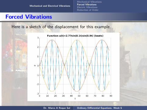
)∣∣∣∣This type of motion, possessing a periodic variation of amplitude,exhibits what is called a beat. In this case ω0 = 1, = 0.8, andF0 = 0.5, so the solution of the given problem is

u(t) = [2.77sin(0.1t)] sin(0.9t)




Forced Vibrations

Here is a sketch of the displacement for this example.




Forced Vibrations

Forced, Damped Vibrations

This is the full blown case where we consider every last possibleforce that can act upon the system. The differential equation forthis case is,

mu′′ + γu′ + ku = F (t)

The displacement function this time will be,

u(t) = uc + UP

where the complementary solution will be the solution to the ( free,damped) homogeneous case and the particular solution will befound using undetermined coefficients or variation of parameters.




Forced Vibrations

There are a couple of things to note here about this case. First,from our work back in the free, damped case we know that thecomplementary solution will approach zero as t →∞. Because ofthis, the complementary solution is often called the transientsolution in this case.

Also, because of this behavior the displacement will start to lookmore and more like the particular solution as t increases and so theparticular solution is often called the steady state solution orforced response.




Forced Vibrations

Example 61

Take the system from the example 59 and add in a damper thatwill exert a force of 45 Newtons when then velocity is 50 cm/sec.Solution

So, all we need to do is compute the damping coefficient for thisproblem then pull everything else down from the previous problem.The damping coefficient is

Fd = γu′ =⇒ 45 = γ(0.5) =⇒ γ = 90




Forced Vibrations

The IVP for this problem is.

3u′′ + 90u′ + 75u = 10cos(5t); u(0) = 0.2, u′(0) = −0.1

The complementary solution for this example is

u(t) = c1e(−15+10

√2)t + c2e

(−15−10√2)t

For the particular solution we the form will be,

UP = Acos(5t) + Bsin(5t)

Plugging this into the differential equation and simplifying gives us,

405Bcos(5t)− 450Asin(5t) = 10cos(5t)




Forced Vibrations

Setting coefficient equal gives,

UP =1

45sin(5t)

The general solution is then

u(t) = c1e(−15+10

√2)t + c2e

(−15−10√2)t +

1

45sin(5t)

Applying the initial condition gives

u(t) = 0.1986e(−15+10√2)t + 0.0014e(−15−10

√2)t +

1

45sin(5t)




Forced Vibrations

Here is a sketch of the displacement for this example.




Electric Vibrations

Electric Circuits

A second example of the occurrence of second order lineardifferential equations with constant coefficients is their use as amodel of the flow of electric current in the simple series circuitshown below




Electric Vibrations

The current I , measured in amperes (A), is a function of time t.The resistance R in ohms (Ω), the capacitance C in farads (F ),and the inductance L in henrys (H) are all positive and areassumed to be known constants.

The impressed voltage E in volts (V ) is a given function of time.Another physical quantity that enters the discussion is the totalcharge Q in coulombs (C ) on the capacitor at time t. The relationbetween charge Q and current I is

I =dQ

dt




Electric Vibrations

The flow of current in the circuit is governed by Kirchhoff’s secondlaw:

(Gustav Kirchhoff (1824 1- 887) was a German physicist andprofessor at Breslau, Heidelberg, and Berlin. http://www.

britannica.com/biography/Gustav-Robert-Kirchhoff )vspace3mmIn a closed circuit the impressed voltage is equal to the sum of thevoltage drops in the rest of the circuit. According to theelementary laws of electricity, we know that


http://www.britannica.com/biography/Gustav-Robert-Kirchhoff

http://www.britannica.com/biography/Gustav-Robert-Kirchhoff



Electric Vibrations

The voltage drop across the resistor is IR.

The voltage drop across the capacitor is Q/C .

The voltage drop across the inductor is LdI/dt.

Hence, by Kirchhoffs law,

−LdIdt− RI − 1

CQ + E (t) = 0 =⇒ L

dI

dt+ RI +

1

CQ = E (t)




Electric Vibrations

The units for voltage, resistance, current, charge, capacitance,inductance, and time are all related:

1volt = 1ohm × 1ampere = 1coulomb/1farad = 1henry × 1ampere/1second .

Substituting dQdt for I , we obtain the differential equation

Ld2Q

dt+ R

dQ

dt+

1

CQ = E (t)

for the charge Q. The initial conditions are

Q(t0) = Q0, Q ′(t0) = I (t0) = I0




Electric Vibrations

Thus we must know the charge on the capacitor and the current inthe circuit at some initial time t0. Alternatively, we can obtain adifferential equation for the current I by differentiating the aboveequation with respect to t, and then substituting dQ/dt for I . Theresult is

Ld2I

dt2+ R

dI

dt+

1

CI = E ′(t)

with the initial conditions

I (t0) = I0, I ′(t0) = I ′0

it follows from the equation for Q(t) that

I ′0 =E (t0)− RI0 − (1/C )Q0

LDr. Marco A Roque Sol Ordinary Differential Equations. Week 6



Electric Vibrations

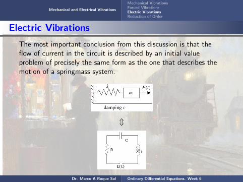
The most important conclusion from this discussion is that theflow of current in the circuit is described by an initial valueproblem of precisely the same form as the one that describes themotion of a springmass system.

m




Reduction of Order

Second Order Lineat Differential Equations. Reduction ofOrder

In the final part of this section, we will consider the general secondorder linear differential equation

y ′′ + p(t)y ′ + q(t)y = g(t)

and introducing new variables, the idea will be to reduce the aboveequation of second order into something of first order.

In that way we propose

x1 = y x2 = y ′




Reduction of Order

these two variables satisfy

x ′1 = y ′ = x2

x ′2 = y ′′ = −p(t)y ′ − q(t)y + g(t) = −p(t)x2 − q(t)x1 + g(t)

therefore, we obtain

x ′1 = x2

x ′2 = −p(t)x2 − q(t)x1 + g(t)

In this way, we have made a reduction of order, but now instead ofa single equation, we have a system linear first oder differentialequations !!!!!




Reduction of Order

Thus, we have showed that a second order linear differentialequations can always be transformed into a system of two linearfirst order differential equations.

OBS

1. The above proposition can be generalized for the n dimensionalcase.

”... An nth order linear differential equation is equivalent to asystem of n linear first order differential equations ...”


Date post:	16-Nov-2021
Category:	Documents
Upload:	others
View:	3 times
Download:	0 times

Ordinary Di erential Equations. Week 6

Documents