ABSTRACT This paper aims to explore the dynamic interaction between the real sector and the financial sector in Malaysia during the period 1986:1 to 2011:4, a period in which the global crisis have been felt. The parsimonious error-correction model (PECM) is used to examine the significant role of financial variables on real output in the long-run as well as in the short-run. The findings suggest the existence of a long-term relationship between the real output and the financial sector. The causality tests reveal that the real output has strong relationships with the real estate and banking sector. From the PECM, the contribution of the banking sector is higher than that from other financial indices. The Kuala Lumpur stock exchange and the real estate contribute the same percentage to the output growth. Meanwhile, financial services accounted a small percentage to the output growth. This finding concludes that the better development in the banking sector stimulates GDP growth in Malaysia. Therefore, for sustainability of output growth, strengthening and establishing a well-developed banking sector is essential. Keywords: real sector, financial sector, the global crisis, vector error correction model (VECM) INTRODUCTION Studies have shown that banks play an important role in promoting the creation of new industries as well as in generating spillover effects on other sectors of the economy (UNDP, 2009, p. 60). Although Malaysia has avoided a financial meltdown during the 2008–2009 Global Financial Crisis (GFC), the contraction in export demand has driven the economy into a recession. Stability in the Malaysian financial sector has been preserved over the period of the GFC. Ample liquidity in the financial system also reduced the risk of systemic spread, allowing the financial sector to continue to provide financial intermediation and services to the economy as a whole. As a highly open economy, Malaysia, however, is not insulated from global economic downturn. Deterioration in the global economy in the second half of 2008 saw the gross domestic product
(GDP) growth of Malaysia moderate to 0.1% in the last quarter of 2008. The domestic economy was experiencing the full impact of the global economic recession in the first quarter 2009, with a decrease of 6.2% in growth. The integrated measures taken by Bank Negara Malaysia (BNM) through the implementation of fiscal stimulus, followed by the easing monetary policy has led to a strong growth of 10.1% in the first quarter of 2010 (Muhammad, 2010).
The aim of this study is to identify the effects of the financial indices namely Kuala Lumpur Stock Exchange, banks, financial services and real estate on the real output in Malaysia. The study focuses on the financial sector because this sector is most affected during the financial crisis (Stiglitz, 1999; Williams & Nguyen, 2005; Kutan, Muradoglu, & Sudjana, 2012). Moreover, the real sector also affected if the significant changes happen in the financial sector. Therefore, assessing both of these sectors is very important. The study raises two questions. First, did the financial sector contribute to the changes in output growth in Malaysia. Second, what is the implication of this relationship to economic growth in Malaysia. The study attempts to shed some lights on the relationship of the sectors and thus contributes new knowledge to the existing literature.
LITERATURE REVIEW The belief that the price of the stock market is related to economic growth has induced research on this link. However, according to Fama (1990), 59% of the variance of annual returns on the value-weighted portfolio of NYSE stocks cannot explain a good or bad news about rationality of stock prices. He also claimed that it is unlikely that a single macro-variable (production) captures all variation in returns due to information about future cash flows. He claimed that a large fraction of the variation of stock returns can be explained, primarily by time variance in expected returns and forecasts of real activity. Although the finding by Fama (1990) is compatible with the study of Lee (1992), where stock return can be used to explain real activity, inflation explains little variation in real activity and the results show a negative correlation between stock returns and inflation. Nevertheless, previous studies showed that inflation contained information on future real activity (Bodie, 1976; Jaffe & Mandelker, 1976; Nelson, 1976; Fama & Schwert, 1977).
In another study concerning the linkages between stock returns and
economic activities of six Asian-Pacific countries, no relationship was found between stock returns and economic variables in the short-term for all the countries under study. However, further study is needed to investigate and identify the potential real variables determining stock returns, particularly in ASEAN countries (Mahmood & Dinniah, 2007). Motivated by the work of
94
Linkages between the real and the Financial Sector
Bilson, Brailsford and Hooper (2001), Samitas and Kenourgios (2007) compared the role of current and future macroeconomic variables in explaining the long-run and short-run stock returns in the 'new' European countries. They used three models to test the validity of the present value model and the relationship between economic variables and stock markets in the European Union. These models incorporate both global and local factors to test whether domestic or foreign factors have greater influence on domestic share prices. Using 1990–2004 quarterly data, the Johansen cointegration test rejects cointegration for all the models in their studies. Furthermore, the long-run structural modeling for domestic and external factors indicates the domestic economy had significant influence on the share prices as compared to external factors. Domestic interest rates were found to have a significant positive influence, which is consistent with the findings of Fama (1990) that the short-term interest rates track economic activity. This implies that an increase in economic activity may cause an increase in stock prices, or in the other words, the shock in the real sector may influence the performance of the financial sector.
Understanding the channels that exist between the financial sector and the real sector in the economy is critically important when assessing financial stability and determining economic performance (Johnston & Pazarbasioglu, 1995). Since the emergence of endogenous growth theory, the importance of financial development has been widely studied (King & Levine, 1993; Demetriades & Luintel, 1996; Denizer, Iyigun, & Owen, 2002). Motivated by the work of King and Levine (1993), Johnston and Pazarbasioglu (1995) tried to examine the importance of the financial sector in determining economic performance. Their study demonstrates that reforms in financial sector have important structural implications in the way financial sector variables affect the real economy. Although some researchers attempted to examine the causality between financial and real sector (Bashir & Hassan, 2002; Denizer et al., 2002; Ang & McKibbin, 2007; Jaafar & Ismail, 2009; Nidhiprabha, 2011), but still, there is no clear consensus regarding the effect of the financial sector on the real sector or vice versa.
A growing body of literature has developed studying the feedback
between the real economy and the financial sector in times of economic shocks. Dovern, Meier and Vilsmeier (2010) noted that the well being of the banking sector can be affected by macroeconomic shocks, but bank lending plays no role in transmitting financial shock to the real sector (Mansor, 2006). In the context of the GFC, Nidhiprabha (2011) asserts that although the real and financial sectors in Thailand are susceptible to adverse impacts of external shock, it had little impact on the financial sector. It can be argued that the result of this finding shows an ambiguity of empirical findings in explaining the impact of external shocks on the real sector and the financial sector in Thailand. Even though the
95
Siti Muliana Samsi et al.
research on financial sector and economic growth have been well documented by previous studies, however, there are no conclusive evidence exist in examining the linkages of the financial sector on the real sector or vice versa. This study attempts to redress this gap by investigating the dynamic interaction between the real sector and the financial sector in Malaysia over the period 1986 to 2011. METHODOLOGY AND MODEL SPECIFICATION Data and Model This study used quarterly data covering the period 1986:1 to 2011:4. The analysis involved four indices and five macroeconomic variables. All the indices of Kuala Lumpur stock exchange (klse), banks (bnk), financial services (fin), real estate (res) and macroeconomic variables of money supply (m), interest rate (r), inflation (p), and exchange rate (e) are exogenous variables while GDP (y) is the endogenous variable. The quarterly data of macroeconomic variables are from the International Financial Statistics compiled by the International Monetary Fund (IMF) and all the indices are obtained from the Datastream database. To investigate the dynamic linkages between the real sector and the financial sector in Malaysia, the following models are used:
Model A: ),,,,,( eprmklseyf = Model B: ),,,,,( eprmbnkyf = Model C: ),,,,,( eprmfinyf =
Model D: ),,,,,( eprmresyf = The above group of models can be represented as a vector error-correction model (VECM), as follows:
Δ y t = α + Σi =1
ρ i
δ 1 iΔ sp t -1 + Σi =1
ρ i
τ 1 iΔm t -1 + Σi =1
ρ i
θ 1 iΔ rt -1 + Σi =1
ρ i
η1 iΔ p t -1
+ Σi =1
ρ i
ψ 1 iΔ e t -1 + ϕ crisis 08 + γECT + ε t
(1)
where sp are price indices of Kuala Lumpur Stock Exchange, banks, financial services and real estate. Whereas y, m, r, p, e, crisis08, and ECT are gross domestic product, money supply, interest rate, inflation, exchange rate, dummy variable of crisis 2008, and error-correction term. The ECT is obtained from the cointegration equation using the Johansen maximum likelihood procedure. All
96
Linkages between the real and the Financial Sector
the series are in logarithmic form except for the interest rate and the exchange rate. Econometric Methodology The most commonly approaches to test for stationarity of time-series data are Augmented Dickey and Fuller (ADF) test, proposed by Dickey and Fuller (1979), and the Phillips Perron (PP) test, proposed by Phillips and Perron (1988). These tests are performed based on the model with a drift and trend (τμ), and, with a drift and without trend (ττ). The purpose of this test is to ensure that all the series should be non-stationary in the levels and stationary after the first difference. For example they should all contain a single unit root. It's also implied that it would be worthwhile to conduct tests of the null hypothesis of mean stationarity in order to determine whether variables are stationary or integrated. Thus, testing for the presence of a unit root is the first step in the empirical investigation before proceed for cointegration.
The number of lag in the vector autoregression (VAR) is used to estimate the cointegrating relationship. It is an important issue because the number of lag shows the number of cointegrating vectors detected. Besides, the long-run and short-run relationships in this study are modeled by using the Johansen and Juselius (1990) and Granger causality framework. The Johansen and Juselius procedure specifies two likelihood ratio test statistics to test the number of cointegrating vectors. These statistics is referred to as λtrace and λmax. The first statistic tests the null hypothesis that the number of distinct cointegrating vectors is less than or equal to r against a general alternative (λtrace equals zero when all i = 0). For the second statistic tests, the null hypothesis that the number of cointegrating vectors is r against the alternative of r + 1 cointegrating vectors. Critical values of the λtrace and λmax statistics are obtained using the Johansen and Juselius approach. The number of lag in the cointegration tests is based on the information provided by the selection of lag length information criteria. Finally, vector error-correction modeling (VECM) is employed to analyse the long-term equilibrium and short-term dynamics of the real sector and the financial sector.
Unit Root Test To test for a unit root (or the difference stationary process), this study employ both the augmented Dickey–Fuller (ADF) and the Phillips–Perron (PP) tests. (a) Augmented Dickey–Fuller regression:
tit
n
iit xpxp εδ +Δ++=Δ −
=− ∑
110tx (2)
97
Siti Muliana Samsi et al.
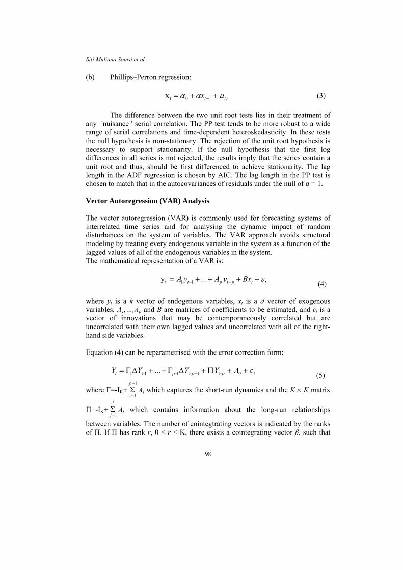
(b) Phillips–Perron regression:
tttx μαα ++= −10tx (3) The difference between the two unit root tests lies in their treatment of
any 'nuisance ' serial correlation. The PP test tends to be more robust to a wide range of serial correlations and time-dependent heteroskedasticity. In these tests the null hypothesis is non-stationary. The rejection of the unit root hypothesis is necessary to support stationarity. If the null hypothesis that the first log differences in all series is not rejected, the results imply that the series contain a unit root and thus, should be first differenced to achieve stationarity. The lag length in the ADF regression is chosen by AIC. The lag length in the PP test is chosen to match that in the autocovariances of residuals under the null of α = 1. Vector Autoregression (VAR) Analysis The vector autoregression (VAR) is commonly used for forecasting systems of interrelated time series and for analysing the dynamic impact of random disturbances on the system of variables. The VAR approach avoids structural modeling by treating every endogenous variable in the system as a function of the lagged values of all of the endogenous variables in the system. The mathematical representation of a VAR is:
ttptpt BxyAyA ε++++= −− ...y 11t (4)
where yt is a k vector of endogenous variables, xt is a d vector of exogenous variables, A1,…,Ap and B are matrices of coefficients to be estimated, and εt is a vector of innovations that may be contemporaneously correlated but are uncorrelated with their own lagged values and uncorrelated with all of the right-hand side variables. Equation (4) can be reparametrised with the error correction form:
tt AYYYY ερρρ ++Π+ΔΓ++ΔΓ= + 0-t1-t1-1-t1 ... (5)
where Γ=-IK+ Aj which captures the short-run dynamics and the K × K matrix
Π=-IK+ Aj which contains information about the long-run relationships
between variables. The number of cointegtrating vectors is indicated by the ranks of Π. If Π has rank r, 0 < r < K, there exists a cointegrating vector β, such that
1
1
−
=Σρ
ii
j 1=Σ
98
Linkages between the real and the Financial Sector
β'Yt is stationary. The existence of cointegration can be factored as Π ≈ αβ' where α and β are (Kxr) matrices. The values of α represent the speed of adjustment in ∆Yt.
To test for the number of cointegrating vectors (β), Johansen and Juselius provide two likelihood ratio (LR) test statistics, namely, the λtrace statistic and the λmax statistic:
)ˆ-ln(1-K
1 iritrace λλ
+=ΣΤ= (6)
)ˆ-(1ln-max 1+Τ= rλλ (7) Where λ�i is the estimated value of characteristic roots obtained from the
estimated Π matrix, K is the number of characteristic root of Π, and Τ is the number of observations. The former tests the null hypothesis that there are at most r distinct cointegrating vectors, while the latter tests the null hypothesis of r cointegrating vectors against the alternative hypothesis of r+1 cointegrating vectors. These statistics have non-standard distributions. Both LR statistics are compared to the critical values tabulated and presented in Johansen and Juselius (1990).
Testing for the absence of a constant in the model requires the estimation
of two models, the restricted model (Ho: without an intercept in cointegrating vector) and the unrestricted model (H1: with an intercept), and use of the test statistic:
(8) r)-(K
2ii
+=~)]ˆ-ln(1-)ˆ-1[ln(ΣΤ- χλλ
K
iri
o
Where Τ is the number of usable observation, K is the number of
characteristic roots of Π, r is the number of non-zero characteristic roots in the unrestricted model, and λ�iº and λ�i are the ordered characteristic roots of the restricted and unrestricted model, respectively. Thus, if the test statistic is sufficiently large, it is possible to reject the null hypothesis concluding that there is an intercept in the cointegrating vector. Vector Error Correction Model (VECM) Testing causality in the VECM framework is presently at the very forefront of econometric research. The underpinnings of this approach demonstrated that once a number of variables (say, xt and yt) are found to be cointegrated, there always exists a corresponding error-correction representation, which implies that changes
99
Siti Muliana Samsi et al.
in the dependent variable are a function of the level of disequilibrium in the cointegrating relationship (captured by the error-correction term, ECT) as well as changes in other explanatory variables. The Granger representation theorem may hypothesise the following testing relationship, which constitutes the VECM given by the equation below:
(9) ∑∑=
−−=
++Δ=Δ1
111 i
ttiti
r
tt
nXAX νθε
Where Xt is an n × 1 vector of variables cointegrated of order r; the A 's are estimable parameters, Ө contains the r individual ECTs derived from the r long-run cointegrating vectors via the Johansen-Juselius (JJ) maximum likelihood procedure (Johansen & Juselius, 1990); ∆ is a difference operator, εi is a vector of impulses, which represent the unanticipated movements in Xt.
In addition to indicating the direction of causality amongst variables, the VECM approach allows us to distinguish between 'short-run' and 'long-run' forms of Granger causality. When the variables are cointegrated, in the short-term, deviations from this long-run equilibrium will feed back on the changes in the dependent variable in order to force the movement towards the long-run equilibrium. EMPIRICAL FINDINGS Unit Root Test The stationarity of the series was investigated by employing the unit root tests developed by Dickey and Fuller (1979), and Phillips and Perron (1988). The joint use of both tests tries to overcome the common criticism that unit root tests have limited power in finite samples to reject the null hypothesis of nonstationarity. Table 1 reports the augmented ADF and PP test statistics for the log levels and first differences. The results of the ADF and PP tests in Table 1 show that all variables contain a unit root, implying that the null hypothesis of the presence of a unit root at level form cannot be rejected even at the 1% significance level. Since all the variables are found to be non-stationary at level, the first differences for all the variables are analysed. The same tests are applied to the first differences and the results show that all the variables become stationary after differencing once. This result demonstrates that all variables are integrated of order one, I(1) and, therefore, we can proceed to the cointegration analysis.
100
Linkages between the real and the Financial Sector
Table 1 Unit Root Test
Bivariate Cointegration Test Table 2 shows the cointegration relationship between real output and the financial indices. The null hypothesis model B, C and D of no cointegration against the alternative of one or more cointegrating vectors (r ≤ 1) is rejected since λmax and λtrace statistics exceeds the critical values at the 1% and 5% significance level respectively. This means that there are two cointegrated equations in Model B, C and D. However, cointegrating vectors (r ≤ 0) is rejected since λmax and λtrace statistics exceeds the critical values at 1% significance level for Model A, and it indicates that there is one cointegrated equation in Model A. Since there exists a cointegration relationship between real output and the financial indices of Kuala Lumpur stock exchange, banks, financial services and real estate, further analysis is performed to identify the linkages and causality between the real output and the financial indices in Malaysia.
101
Siti Muliana Samsi et al.
Table 2 Johansen Cointegration Test (bivariate analysis)
Max Eigenvalue Statistic Trace Statistic (λ trace) (λ max)
r ≤ 1 r ≤ 1 k r = 0 r = 0
Vector : [y, klse] 21.42630a 3.311220 18.11508b Model A 6 3.311220
Vector : [y, bnk] 22.30567a 6.498538b 15.80713b 6.498538b Model B 6
Vector : [y, fin] 20.70042a 5.790571b 14.90985b 5.790571b Model C 6 Vector : [y, res] 21.97258a 6.960113a 15.01247b 6.960113a Model D 6
Note: a and b denote significant at 1% and 5% levels respectively. λ trace and λ max are the likelihood ratio statistics for the number of cointegrating vectors. The lag length (k) was selected based on Akaike Information Criteria (AIC).
VAR Granger Causality/Block Exogeneity Wald Tests The Granger causality test in Table 3 reveals that the indices of Kuala Lumpur stock exchange and financial services are not significantly Granger caused by real output. This implies there is no causality running from real output to Kuala Lumpur stock exchange, and real output to financial services. The study finds that there are bidirectional causality between real output to the real estate, and real output to the banks indices. Since the results of λ² (chi-sq) is statistically significant at 1 and 5 percent level, real output in Malaysia has a strong relation with the real estate and banking sector. Therefore, the study carry on with the multivariate cointegration test (Table 4) and parsimonious error-correction model (Table 5) to gain more insight into the role of real output and financial variables in Malaysia.
102
Linkages between the real and the Financial Sector
Table 3 VAR Granger Causality/Block Exogeneity Wald Tests
Regression λ2 (Chi-sq) Prob
Model A [y, klse] Δy on Δklse 8.510705 [0.2030] Δklse on Δy 29.51764 [0.0000] Model B [y, bnk] Δy on Δbnk 7.093987 [0.0288] Δbnk on Δy 10.50435 [0.0052] Model C [y, fin] Δy on Δfin 10.32112 [0.1118] Δfin on Δy 38.13118 [0.0000] Model D [y, res] Δy on Δres 12.70316 [0.0480] Δres on Δy 31.08507 [0.0000]
Multivariate Cointegration Test Table 4 reports on the multivariate cointegration test for real output, money supply, interest rate, inflation, exchange rate, Kuala Lumpur stock exchange, banks, financial services and real estate. The null hypothesis of models A and D of no cointegration against the alternative of one cointegrating vector (r ≤ 1) is rejected since λmax and λtrace statistics exceed the critical values at 5% significance level for these models, and cointegrating vectors (r ≤ 1) is rejected since λmax exceed the critical value at 5% significance level for the Model B. Moreover, cointegrating vectors (r = 0) is rejected since λtrace and λmax statistics exceeds the critical values at 5% significance level for the Model C, and cointegrating vectors (r = 0) is rejected since λtrace exceeds the critical value at 5 percent significance level for Model B. This means that there are two cointegrated equations in Model A, B and D. The empirical analyses also assume that there is one cointegrated equation in Model C. Further analysis of parsimonious error-correction model (PECM) is used in this study to examine the significant role of the financial variables on the real output in the long-run as well as in the short-run.
103
Siti Muliana Samsi et al.
Table 4 Johansen Cointegration Test (multivariate analysis)
Parsimonious Error-Correction Model (PECM) Table 5 presents the results obtained from the PECM for the sample period 1986:1 to 2011:4. The number of lags in the ECM is similar to the number of lags that used in the contegration test. The purpose of this analysis is to identify the significant role of the financial variables to the real sector in Malaysia.
In Table 5, the equation in Model A is estimated with five lags and two cointegrating vectors. The speed of adjustment to the long-run equilibrium level is shown by ECT. The coefficient of ECT is negative and significant; indicating that real output adjusts to bring about the long-run equilibrium by closing 1.95% of the gap. Even though the real output is influenced by the financial variables in the short-run as well as in the long run, the role that is played by money supply M2 is dominant as compared to other financial variables. The money supply has a supply growth will bring about a 0.21% change in output growth. Moreover, a
104
Linkages between the real and the Financial Sector
dummy variable CRISIS08 is introduced to represent the impact of the GFC. The findings show that real output is affected by the GFC.
In Model B, the coefficient of money supply is positive and significant at
two-quarter lag with the elasticity at 0.22. The adjustment coefficient is 2.41% and is higher than in Model A. The negative and significant ECT indicates that real output adjusts to clear the disequilibrium to the long-run equilibrium through the 2.41% speed of adjustment. The dummy coefficient CRISIS08 is negative and significant in this equation, meaning that the GFC had a significant effect on the growth of real output.
As can be seen in Model C, the money supply at two-quarter lag and
three-quarter lag is elastic in the range of 0.15–0.23. The coefficient of ECT shows that the speed of adjustment of real output towards the long-run equilibrium level is 3.11%. Moreover, CRISIS08 is important and has a negative sign which implies that the greater the crisis, the larger the output growth falls.
The empirical results of Model D in Table 5 show that the money supply
is significant at two-quarter lag. The elasticity of money supply is 0.27. From the long-run impact, the real output moves to eliminate the discrepancy between the short-run and the long-run equilibrium through closing 2.85% of the gap. Furthermore, the dummy variable CRISIS08 shows that real output is affected by the GFC. The crisis has led to the decline in growth of real output.
The result for each model confirms that from diagnostic tests, there is
insignificant evidence of serial correlation and heteroskedasticity, which indicates that the residuals are normally distributed. The regression specification error test (RESET) shows that all the models are correctly specified. Moreover, the test of normality using cumulative sum (CUSUM) and cumulative sum of squares (CUSUMQ) do not find any instability or major structural changes in each model.
The results given by PECM generally show the money supply entering the equation significantly at 1%, 5% and 10% level with the expected positive sign. In particular, the elasticity of money supply with respect to real output is 0.21 for Model A, 0.22 for Model B, 0.15–0.28 for Model C, and 0.27 for Model D (Table 5). The empirical analysis shows that the money supply has a strong relationship with real output growth. This relation is due to the sticky-wage theory with unanticipated changes in money (Fischer, 1977; Taylor, 1980). The theory explains that the changes in growth of the money supply cause changes in output growth. Moreover, the monetary aggregate can be the most suitable target to sustain economic growth because it contains information about output and prices (Favara & Giordani, 2009).
105
Siti Muliana Samsi et al.
Table 5 Parsimonious Error–Correction Model (PECM)
106
Linkages between the real and the Financial Sector
107
Siti Muliana Samsi et al.
108
Linkages between the real and the Financial Sector
109
Siti Muliana Samsi et al.
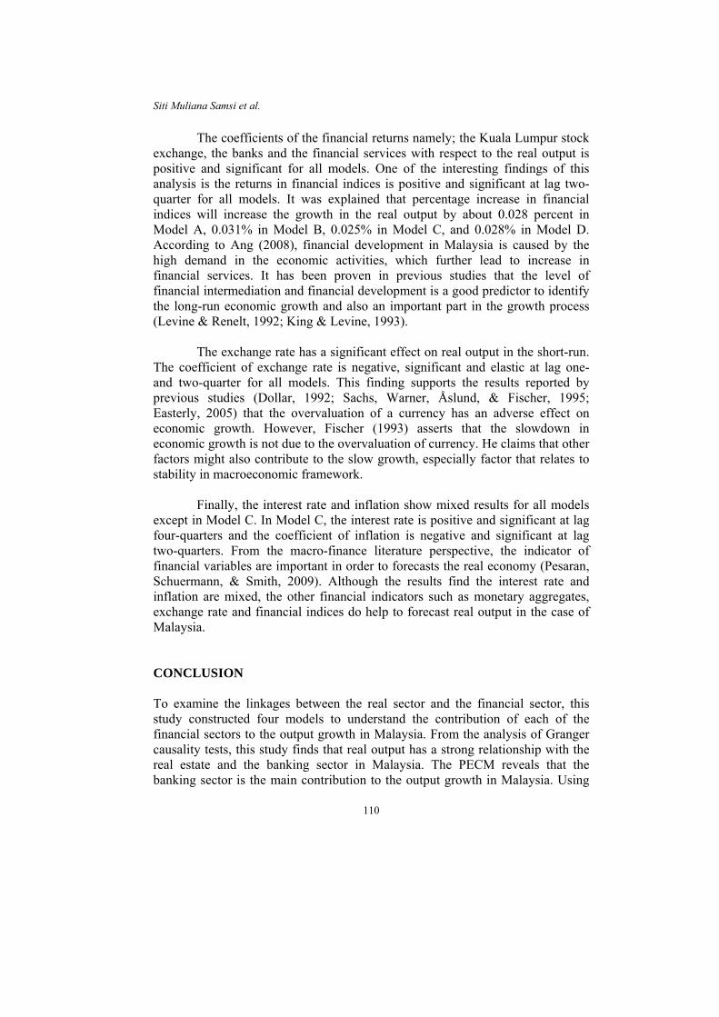
The coefficients of the financial returns namely; the Kuala Lumpur stock exchange, the banks and the financial services with respect to the real output is positive and significant for all models. One of the interesting findings of this analysis is the returns in financial indices is positive and significant at lag two-quarter for all models. It was explained that percentage increase in financial indices will increase the growth in the real output by about 0.028 percent in Model A, 0.031% in Model B, 0.025% in Model C, and 0.028% in Model D. According to Ang (2008), financial development in Malaysia is caused by the high demand in the economic activities, which further lead to increase in financial services. It has been proven in previous studies that the level of financial intermediation and financial development is a good predictor to identify the long-run economic growth and also an important part in the growth process (Levine & Renelt, 1992; King & Levine, 1993).
The exchange rate has a significant effect on real output in the short-run.
The coefficient of exchange rate is negative, significant and elastic at lag one- and two-quarter for all models. This finding supports the results reported by previous studies (Dollar, 1992; Sachs, Warner, Åslund, & Fischer, 1995; Easterly, 2005) that the overvaluation of a currency has an adverse effect on economic growth. However, Fischer (1993) asserts that the slowdown in economic growth is not due to the overvaluation of currency. He claims that other factors might also contribute to the slow growth, especially factor that relates to stability in macroeconomic framework.
Finally, the interest rate and inflation show mixed results for all models
except in Model C. In Model C, the interest rate is positive and significant at lag four-quarters and the coefficient of inflation is negative and significant at lag two-quarters. From the macro-finance literature perspective, the indicator of financial variables are important in order to forecasts the real economy (Pesaran, Schuermann, & Smith, 2009). Although the results find the interest rate and inflation are mixed, the other financial indicators such as monetary aggregates, exchange rate and financial indices do help to forecast real output in the case of Malaysia.
CONCLUSION To examine the linkages between the real sector and the financial sector, this study constructed four models to understand the contribution of each of the financial sectors to the output growth in Malaysia. From the analysis of Granger causality tests, this study finds that real output has a strong relationship with the real estate and the banking sector in Malaysia. The PECM reveals that the banking sector is the main contribution to the output growth in Malaysia. Using
110
Linkages between the real and the Financial Sector
the PECM leads to the interesting finding that the returns in financial indices are positive and significant at lag two-quarter for all models. The study finds that the contribution of the banking sector to growth is higher than that of other financial indices. The Kuala Lumpur stock exchange and real estate contribute the same percentage to the output growth. Meanwhile, financial services only contributed a little to output growth. Thus, further development of the banking sector will stimulate GDP growth in Malaysia. REFERENCES Ang, J. B. (2008). Are financial sector policies effective in deepening the Malaysian
financial system? Contemporary Economic Policy, 26(4), 623–635. Ang, J. B., & McKibbin, W. J. (2007). Financial liberalization, financial sector
development and growth: Evidence from Malaysia. Journal of Development Economics, 84(1), 215–233.
Bashir, A., & Hassan, M. (2002). Financial development and economic growth in the middle east. Working Paper, University of New Orleans
Bilson, C. M., Brailsford, T. J., & Hooper, V. J. (2001). Selecting macroeconomic variables as explanatory factors of emerging stock market returns. Pacific-Basin Finance Journal, 9(4), 401–426.
Bodie, Z. (1976). Common stocks as a hedge against inflation. The Journal of Finance, 31(2), 459–470.
Demetriades, P. O., & Luintel, K. B. (1996). Financial development, economic growth and banking sector controls: Evidence from India. The Economic Journal, 106(435), 359–374.
Denizer, C. A., Iyigun, M. F., & Owen, A. (2002). Finance and macroeconomic volatility. The BE Journal of Macroeconomics, 2(1), 1–30.
Dickey, D. A., & Fuller, W. A. (1979). Distribution of the estimators for autoregressive time series with a unit root. Journal of the American Statistical Association, 74(366), 427–431.
Dollar, D. (1992). Outward-oriented developing economies really do grow more rapidly: Evidence from 95 LDCs, 1976-1985. Economic Development and Cultural Change, 40(3), 523–544.
Dovern, J., Meier, C. P., & Vilsmeier, J. (2010). How resilient is the German banking system to macroeconomic shocks? Journal of Banking & Finance, 34(8), 1839–1848.
Easterly, W. (2005). National policies and economic growth: A reappraisal. Handbook of Economic Growth, 1, 1015–1059.
Fama, E. F. (1990). Stock returns, expected returns, and real activity. The Journal of Finance, 45(4), 1089–1108.
Fama, E. F., & Schwert, G. W. (1977). Asset returns and inflation. Journal of Financial Economics, 5(2), 115–146.
Favara, G., & Giordani, P. (2009). Reconsidering the role of money for output, prices and interest rates. Journal of Monetary Economics, 56(3), 419–430.
111
Siti Muliana Samsi et al.
Fischer, S. (1977). Long-term contracts, rational expectations, and the optimal money supply rule. The Journal of Political Economy, 85(1), 191–205.
Fischer, S. (1993). The role of macroeconomic factors in growth. Journal of Monetary Economics, 32(3), 485–512.
Gonzalo, J. (1994). Five alternative methods of estimating long-run equilibrium relationships. Journal of Econometrics, 60(1-2), 203–233.
Jaafar, P., & Ismail, A. (2009). Dynamic relationship between sector-specific indices and macroeconomic fundamentals. Malaysian Accounting Review, 8(1), 81–100.
Jaffe, J. F., & Mandelker, G. (1976). The "Fisher Effect" for risky assets: An empirical investigation. The Journal of Finance, 31(2), 447–458.
Johansen, S., & Juselius, K. (1990). Maximum likelihood estimation and inference on cointegration, with applications to the demand for money. Oxford Bulletin of Economics and Statistics, 52(2), 169–210.
Johnston, R. B., & Pazarbasioglu, C. (1995). Linkages between financial variables, financial sector reform and economic growth and efficiency. IMF Working Paper No. 95/103.
King, R. G., & Levine, R. (1993). Finance and growth: Schumpeter might be right. The Quarterly Journal of Economics, 108(3), 717–737.
Kutan, A. M., Muradoglu, G., & Sudjana, B. G. (2012). IMF programs, financial and real sector performance, and the Asian crisis. Journal of Banking & Finance, 36(1), 164–182.
Lee, B. S. (1992). Causal relations among stock returns, interest rates, real activity, and inflation. The Journal of Finance, 47(4), 1591–1603.
Levine, R., & Renelt, D. (1992). A sensitivity analysis of cross-country growth regressions. The American Economic Review, 942–963.
Mahmood, W. M., & Nazihah, M. D. (2007). Stock returns and macroeconomic influences: Evidence from the six Asian-Pacific countries. International Research Journal of Finance & Economics, 30, 154–164.
Mansor, H. I. (2006). Stock prices and bank loan dynamics in a developing country: The case of Malaysia. Journal of Applied Economics, 9(1), 71.
Muhammad, I. (2010). Impact of the global crisis on Malaysia 's financial system., BIS paper No.54, Bank for International Settlements.
Nelson, C. R. (1976). Inflation and rates of return on common stocks. The Journal of Finance, 31(2), 471–483.
Nidhiprabha, B. (2011). The global financial crisis and resilience of the Thai banking sector. Asian Development Review, 28(2), 110.
Pesaran, M. H., Schuermann, T., & Smith, L. V. (2009). Forecasting economic and financial variables with global VARs. International Journal of Forecasting, 25(4), 642–675.
Phillips, P. C. B., & Perron, P. (1988). Testing for a unit root in time series regression. Biometrika, 75(2), 335.
Sachs, J. D., Warner, A., Åslund, A., & Fischer, S. (1995). Economic reform and the process of global integration. Brookings Papers on Economic Activity, 1995(1), 1–118.
Samitas, A. G., & Kenourgios, D. F. (2007). Macroeconomic factors' influence on 'new' European countries' stock returns: The case of four transition economies. International Journal of Financial Services Management, 2(1), 34–49.
112
Linkages between the real and the Financial Sector
Stiglitz, J. E. (1999). Reforming the global economic architecture: Lessons from recent crises. The Journal of Finance, 54(4), 1508–1522.
Taylor, J. B. (1980). Aggregate dynamics and staggered contracts. The Journal of Political Economy, 88(1), 1–23.
United Nations Development Programme (UNDP). (2009). The global financial crisis and the Malaysian economy: Impact and responses. A joint ISIS and UM report commissioned by the UNDP.
Williams, J., & Nguyen, N. (2005). Financial liberalisation, crisis, and restructuring: A comparative study of bank performance and bank governance in South East Asia. Journal of Banking & Finance, 29(8), 2119–2154.