48
Linking CGE model to pollution emission
| Date post: | 01-Apr-2018 |
| Category: |
Documents |
| Upload: | truongnhan |
| View: | 215 times |
| Download: | 0 times |

Linking CGE model to pollution
emission

What is a single country CGE
model

Walrasian general equilibrium prevails when supply and
demand are equalized across all of the interconnected markets
in the economy.
CGE models are simulations that combine the abstract general
equilibrium structure of Arrow and Debreu with realistic
economic data to solve numerically.
CGE models are a standard tool of empirical analysis, and are
widely used to analyze the aggregate welfare and distributional
impacts of policies whose effects may be transmitted through
multiple markets, or contain menus
of different tax, subsidy, quota or transfer instruments.
What is a CGE model

4
• Input Output Economics & SAMs
• Behavioral Relationships/ Agents – Supply
– Demand
– Trade
• Government
• Pricing
• Policy – tax equivalents
• Closure – Accounting identities
– Endogenous/exogenous variables
– Macroeconomic assumptions
– Exchange rate determination
• Solution – Equilibrium
– Linearization
– Percent change variables
CGE Standard Model Elements

5
CGE Standard Model Elements
• Calibration/Benchmarking
• Aggregation
– Agents
– Goods/Sectors
• Experiments
– Welfare Measures
– Projections
– What if
• Extensions
– Imperfect Competition, IRS
– Product Differentiation
– Dynamics
• Results Comparisons

6
Input-Output economics & SAMs
• Production= Intermediates + Value Added
• Production= Intermediate demand + Final Demand
• +
• Macroeconomic accounting identities to capture income flows, tax incidence, trade and payments, and savings-investment balances
• = > SAMs capture `circular flow’ of income and expenditure

7
• A social accounting matrix to benchmark
(calibrate) a model and to represent relevant
accounting identities.
• SAMs capture equilibrium conditions
• Walras’ law applies
Input-Output economics & SAMs

8
Decision Making and Institutions
• Linkages in SAMs are accounted for by
modelling the decision-making process of the
firm, the consumer, as well as other economic
agents and institutions: production and demand
structure
• Trade results from that decision-making
processes and their interaction with
institutions:
• Production- Exports +
Imports=Consumption

9
Closing the Model
• Need to define a numéraire (walras law allows
to “drop” one market)
• Assumption about the adjustment mechanism
in factor and commodity markets
• Macro closure
– Macro accounting balance (gvt expenditure and
deficit; aggregate saving and investment; balance
of trade and -real- exchange rate)
– Macro adjustment mechanism (exogenously
determined)

Payments
Product Markets
Factor Markets
Government
Goods &
Services
Goods &
Services
Taxes Taxes
Goods &
Services
Profits/ Factor Income
Expenditure
Households Firms
Factor
Inputs
Prod 1
Prod2
Prod n
Goods and factors
Capital
Labor
Natural resources
Natural resources

11
CGE Dynamic Models
• Recursive:
Capital stock
governance
structure
Structural
reforms
Intermediate
consumption
Period t
equilibrium
Change in factor
endowment (labor, capital)
Change in fiscal policy
Period t+1
equilibrium
The Model
Labor stock
Capital stock
Intermediate
consumption
Labor stock

Mirage Global CGE model

Product Markets
Factor Markets
Government
Goods &
Services
Goods &
Services
Taxes Taxes
Goods &
Services
Profits/ Factor Income
Expenditure
Households Firms
Factor
Inputs
Prod 1
Prod2
Prod n
What is a Global CGE model: A 2 countries model
International
Financial
market
Capital
Labor
Natural
resources
land
Product Markets
Factor Markets
Government
Goods &
Services
Goods &
Services
Taxes Taxes
Goods &
Services
Profits/ Factor Income
Expenditure
Households Firms
Factor
Inputs
International
G & S
Market
International
factors
market
Country A Country B
International
transport
Data
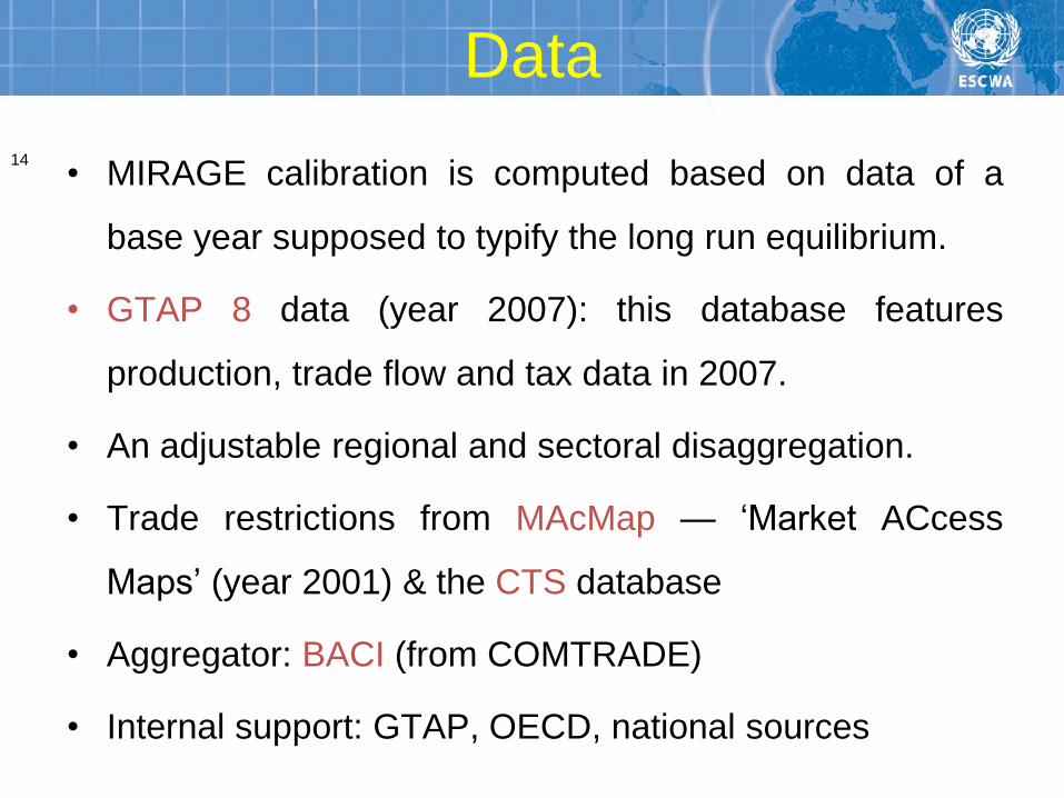
14
• MIRAGE calibration is computed based on data of a
base year supposed to typify the long run equilibrium.
• GTAP 8 data (year 2007): this database features
production, trade flow and tax data in 2007.
• An adjustable regional and sectoral disaggregation.
• Trade restrictions from MAcMap — ‘Market ACcess
Maps’ (year 2001) & the CTS database
• Aggregator: BACI (from COMTRADE)
• Internal support: GTAP, OECD, national sources

Production
Supply (1)
15
(see below: Added Value)
(see below: Demand)
Good 1 Good 1 Good n
Leontieff
Value
added
Intermediate
consumption

Supply (2)
Unskilled
labour
Skilled
labour
Capital
Composite
factor
Natural
resources
Land
Added value
16
Cobb-Douglas
CES 0.6
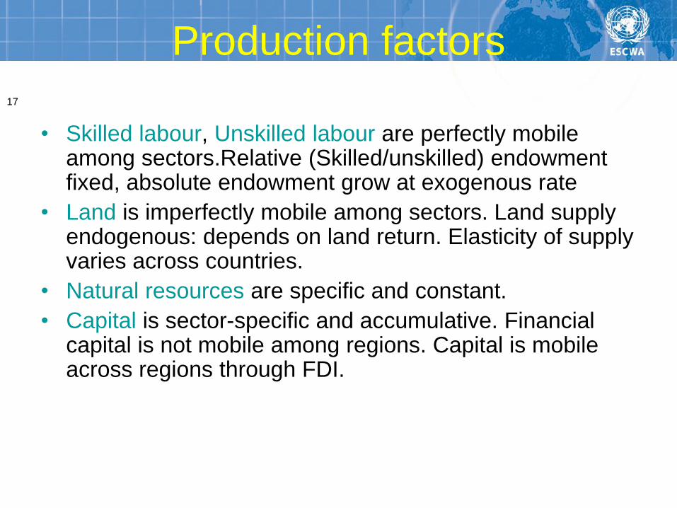
Production factors
17
• Skilled labour, Unskilled labour are perfectly mobile among sectors.Relative (Skilled/unskilled) endowment fixed, absolute endowment grow at exogenous rate
• Land is imperfectly mobile among sectors. Land supply endogenous: depends on land return. Elasticity of supply varies across countries.
• Natural resources are specific and constant.
• Capital is sector-specific and accumulative. Financial capital is not mobile among regions. Capital is mobile across regions through FDI.

Demand
18
• 3 types of demand: final consumption, intermediate consumption and capital good.
• Goods are distinguished by origin with several levels:
- differentiation according to quality;
- differentiation local vs. foreign;
- differentiation by regions within each quality zone.
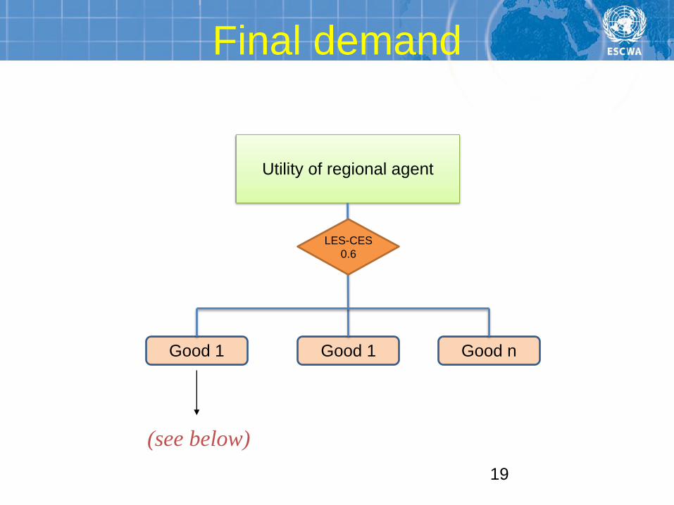
Final demand
19
(see below)
Utility of regional agent
Good 1 Good 1 Good n
LES-CES
0.6

Capital good
20
(see below)
Capital good
Good 2 Good 1 Good n
CES 0.6

Choice of goods among production location
Titre du diagramme
Local
Region 1 Region 2
Foreign
Zone u
Region 3 Region 4
Zone v
Good i
21
CES GEO
CES ARM CES IMP
CES IMP
Where GEO= (ARM -1) /2 1/2 +1 and ARM= (IMP -1) /2 1/2 +1

Capital and investment
24 • Installed capital is assumed to be immobile and sector-specific.
• Accordingly, the rate of return to capital may vary across sectors and regions
• Domestic and foreign investments are the only adjustment device for capital stocks
• Portfolio allocation strategy
• Because the existence of a risk, which is not explicitly modelled, substitution between the different assets is not perfect.
• A single formulation is used for setting both domestic and foreign investment.

Financial closure
27
• The saving rate is constant. Savings finance local investment and FDI-out.
• External credit to the regional agent is exogenous.
• So the Current account balance varies according to the difference between the FDI-in and FDI-out
Current account = FDI in – FDI out + External credit exogenous

Sequential Dynamics
29
• Dynamics is a succession of static equilibrium states.
• Some parameters and exogenous variables change from
one period to the next:
– factor stocks
– economic policy.
• Capital evolves endogenously through investment
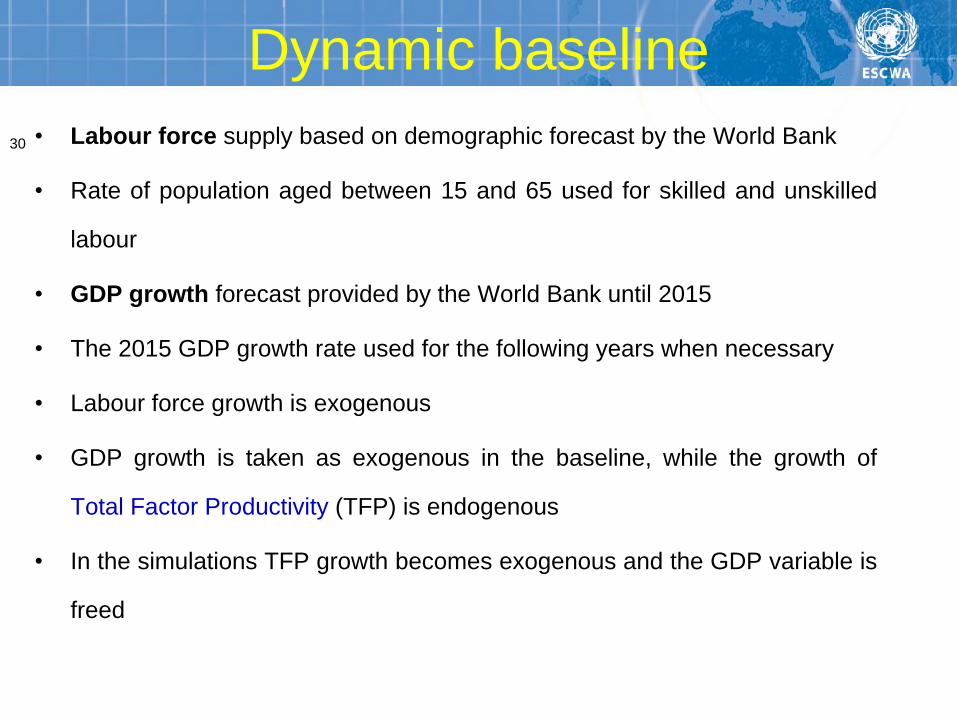
Dynamic baseline
30 • Labour force supply based on demographic forecast by the World Bank
• Rate of population aged between 15 and 65 used for skilled and unskilled
labour
• GDP growth forecast provided by the World Bank until 2015
• The 2015 GDP growth rate used for the following years when necessary
• Labour force growth is exogenous
• GDP growth is taken as exogenous in the baseline, while the growth of
Total Factor Productivity (TFP) is endogenous
• In the simulations TFP growth becomes exogenous and the GDP variable is
freed
How to introduce CO2
emission in Mirage

Taking into consideration energy consumption in the production
function
Production of sector (i) in
country (r)
Leontieff
Value
added
Intermediate
consumption
Good
1
Good
2
Good
n
Non energy commodities
coal Crude
oil
Natural
gas
Petroleum
products
electri
city
Gas
distribution
energy commodities
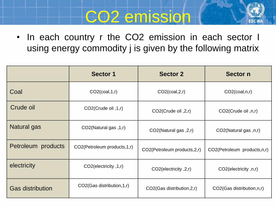
CO2 emission • In each country r the CO2 emission in each sector I
using energy commodity j is given by the following matrix
Sector 1 Sector 2 Sector n
Coal CO2(coal,1,r) CO2(coal,2,r) CO2(coal,n,r)
Crude oil
CO2(Crude oil ,1,r)
CO2(Crude oil ,2,r) CO2(Crude oil ,n,r)
Natural gas
CO2(Natural gas ,1,r)
CO2(Natural gas ,2,r) CO2(Natural gas ,n,r)
Petroleum products
CO2(Petroleum products,1,r)
CO2(Petroleum products,2,r) CO2(Petroleum products,n,r)
electricity
CO2(electricity ,1,r)
CO2(electricity ,2,r) CO2(electricity ,n,r)
Gas distribution CO2(Gas distribution,1,r)
CO2(Gas distribution,2,r) CO2(Gas distribution,n,r)

In MIRAGE and GTAP

Values of coefficients

Assessing the CO2 impacts of an economic policy
The CGE model
Trade
liberalization
Fiscal reform
Subsidies
elimination
Productivity
choc
welfare
Fiscal
impacts
CO2
emission
effects
Growth
Economic external
choc
Health
impacts
Market access
impacts
First order
economic impacts
Application: Local Air Pollution and Public Health in
Tunisia: Assessing the Ancillary Health Benefits of
Pollution Abatement Policy
38

39
There has been an explosion of interest in the potential benefits of pollution
abatement to offset some of the costs of reducing gas emissions.
While the list of such effects is long and the benefits from each are large,
pollution will yield far better deal when these benefits are captured
Until quite recently, literature on direct and ancillary benefits, came from
developed countries, especially the US and Europe.
In the Arab region, no empirical analysis tried to estimate ancillary benefits of
pollution abatement policies.
INTRODUCTION AND OBJECTIVES

40
What interest do developing countries have in limiting the growth of their
greenhouse gas (GHG) emissions or other pollutants?
The primary benefits for individual countries of GHG abatement remain highly
uncertain, and, in any case, long term in nature. The costs, on the other
hand, are near-term. However, the benefits of reducing emissions of many
pollutants, also associated with energy consumption, is immediate.
Four categories of effects of pollution abatement policies have been
identified: Health, ecological, economic, and social.
In addition to considering the full range of sources of benefits, it is also vital to
consider costs
INTRODUCTION AND OBJECTIVES

41
METHODOLOGICAL CONSIDERATIONS
Making estimates of ancillary benefits involves carefully following the chain linking a
specific policy measure to changes in emissions levels to changes in ambient
pollutant concentration to changed human (or animal or plant or material) exposure
to environmental/health effects and finally to monetized welfare changes
Each link in this chain involves difficult measurement/estimation problems

42
Links in Chain from Policy Measure to Welfare Change
Policy change (e.g. pollution tax) →
Emissions reduction →
Lower ambient concentration →
Reduced exposure →
Improved health →
Welfare gains.

METHODOLOGY
• The standard CGE model has been extended to incorporate additional
features for the analysis of ancillary benefits of pollution abatement
policy. The main changes are the following:
• 1. Energy types (production functions and final demands)
• 2. Modeling emissions
• 3. Modeling the links between emissions, ambient concentration and
exposure
• 3. Modeling health effects
• 4. Modeling Pollution Abatement tax
• 5. Modeling welfare change with reduced health damages
43

I. METHODOLOGY (4)
• Additional data used for the CGE model:
• 1. Sectoral emission intensities for production
• 2. Sectoral emission intensities for consumption
• 3. Monetary Values Estimates of Unit Changes in various health
endpoints
44

Sectoral emission intensities for production – 2006
(metric tons per millions TD)
45
Agri Chemicals Textiles Other Manufacturing Non Manufacturing
Industries
Services
TOXAIR 9,5 180,7 56,3 37,8 33,7 6
TOXWAT 18,8 464,1 11,7 73,9 45,6 12,4
TOXSOL 17,8 562,2 11,5 159,2 235,5 16,8
BIOAIR 28,2 515,1 12,9 395,8 670,5 28,9
BIOWAT 0,3 25,8 0,3 16,6 32,2 1,1
BIOSOL 294,1 10374,6 171 7198,7 13188,9 505,9
SO2 17,9 493,2 11,4 64,7 39,8 11,5
NO2 11 298,1 77 37,3 18,9 6,8
CO 6,8 209,7 4,5 48,5 52,8 5,5
VOC 16 318,5 7,3 46,1 32,8 7,6
PART 3 82,4 1,9 12 5,8 1,9
BOD 7,9 17,4 0,2 13,8 21,8 0,8
TSS 9,5 966,4 10 621,5 1198,7 41,8
Output% 7,7 4,1 7,9 24,3 16,9 39,1
Exp/Output 7,3 47,3 85,7 34,7 15,7 7,8
Imp/Demand 30,7 191,9 159,1 104,1 156,3 131,9

Sectoral emission intensities for consumption – 2006
(metric tons per millions TD)
46
AgriFood Chemicals Textiles Other Manufacturing Non Manufacturing
Industries
Services
TOXAIR 0 301,2 0 23,9 0 0
TOXWAT 0 856,6 0 10 0 0
TOXSOL 0 752,8 0 42,5 0 0
BIOAIR 0 0 0 214,5 0 0
BIOWAT 0 0 0 4,9 0 0
BIOSOL 0 0 0 2929,6 0 0
SO2 0 925,4 0 4,7 0 0
NO2 0 567,8 0 2 0 0
CO 0 335,9 0 7,5 0 0
VOC 0 586,3 0 4,1 0 0
PART 0 155,9 0 0,7 0 0
BOD 0 0 0 3,3 0 0
TSS 0 0 0 180,7 0 0
Cons % 10 3 4 11 12 60
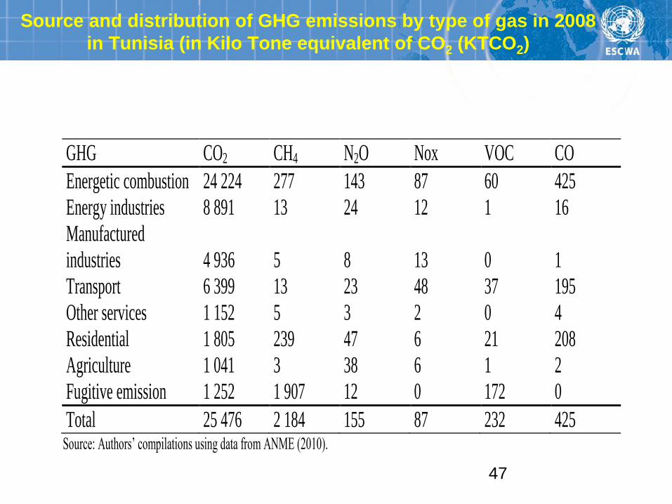
Source and distribution of GHG emissions by type of gas in 2008
in Tunisia (in Kilo Tone equivalent of CO2 (KTCO2)
47
GHG CO2 CH4 N2O Nox VOC CO
Energetic combustion 24 224 277 143 87 60 425
Energy industries 8 891 13 24 12 1 16
Manufactured
industries 4 936 5 8 13 0 1
Transport 6 399 13 23 48 37 195
Other services 1 152 5 3 2 0 4
Residential 1 805 239 47 6 21 208
Agriculture 1 041 3 38 6 1 2
Fugitive emission 1 252 1 907 12 0 172 0
Total 25 476 2 184 155 87 232 425 Source: Authors’ compilations using data from ANME (2010).

Major Air Pollutants, Their Sources and Their
Environmental Impacts
48
Pollutant Major Sources Transformations in
Atmosphere
Major End-Points Nature of Effects
Particulates
Sulphur dioxide
(SO2) and sulphate
aerosols (SO4)
Nitrogen oxides
(NOX) and nitrates
(NO2 and HNO3)
Volatile organic
compounds (VOCs)
Ozone (O3)
Lead (Pb)
Carbon monoxide
(CO)
Fossil fuel combustion
(exc. Natural gas)
construction, natural dust (small proportion
inhalable)
Coal and diesel fuel
combustion
Fuel combustion
Fuel combustion
Gasoline
Fuel combustion,
including biomass
SO2 transported,
transformed into and
suspended/deposited as
SO4
Precursor to acid rain;
Constituent in formation
of photochemical smog
and of tropospheric O3
Constituent in formation
of photochemical smog
Formed from oxidation of
NOX in the presence of
sunlight and reactive
VOCs
(i) Health
(ii) Materials
(i) Health
(ii) Soils, forests,
aquatic ecosystems
i) Health
ii) Visibility
i) Visibility
ii) Health
Health
Health
Health
a) Mortality
b) Morbidity: respiratory
and cardiovascular
complications
c) Soiling
a) Mortality
b)Morbidity: respiratory
illness Acidification
Respiratory problems
Reduced enjoyment
Reduced amenity value
Cancer
Acute respiratory distress at
high concentrations (asthma)
a)Adults: hypertension;
stroke
b) Children: Reduced IQ
a) Asphyxiation
b) Stillbirth

Air Quality Standards in Tunisia
49
Average
type
Exceeding authorisation Limiting value
(related to health)
Guide value (related to
welfare)
CO 8 hours 2 times/30 days 9 ppm- 10 mg/m3 9 ppm- 10 mg/m
3
1 hour 2 times/30 days 35 ppm- 40 mg/m3 26 ppm- 30 mg/m
3
NO2 Annual
average
- 0.106 ppm- 200 mg/m3 0.08 ppm- 150 mg/m
3
1 hour 1 time/30 days 0.35 ppm- 660 mg/m3 0.212 ppm- 400 mg/m
3
O3 1 hour 2 times/30 days 0.12 ppm- 235 mg/m3 0.077-0.102 ppm- 150 to
200 µg/m3
Suspended
particulate
(PM 10)
Annual
average
- 80 µg/m3 40 to 60 µg/m
3
24 hours 1 time/ 12 months 260 µg/m3 120 µg/m
3
SO2 Annual
average
- 0.03 ppm- 80 µg/m3 0.019 ppm- 50 µg/m
3
24 hours 1 time/ 12 months 0.12 ppm- 365 µg/m3 0.041 ppm- 125 µg/m
3
3hours 1 time/ 12 months 0.5 ppm- 1300 µg/m3 -
Pb Annual
average
- 2 µg/m3 0.5 to 1 µg/m
3
H2S 1 hour 1 time/ 12 months 200 µg/m3 -
Source: ANPE (2008).

Solid Particulate concentration in selected Tunisian
cities PM10 (2004-2008) in (µg/m3)
50
PM10 2004 2005 2006 2007 2008
Av/year 24 h Av/year 24 h Av/year 24 h Av/year 24 h Av/year 24 h
Bab Saâdoun 85 526 82 195 88 316 91 328 77 190
Bizerte 83 466 91 249 98 711 80 248 67 216
Sfax city - - - 197 87 318 87 240 90 335
Ben Arous - - - - 78 141 81 279 74 183
Sousse - - - 105 54 181 57 172 55 143
Sfax south
suburban
- - 180 117 94 582 90 264 89 326

Monetary Values Estimates of Unit Changes in
various health endpoints
51
Equivalent
estimate for
Tunisia, 2020
Units
Value of statistical life (VSL)
Respiratory hospital admission (RHA)
Emergency room visit (ERV)
Restricted activity day (RAD)
Minor restricted activity day (MIRAD)
Clinic visit for LRI in children
Chronic bronchitis in adults
Asthma attack
Respiratory symptom day
Child respiratory symptom day
Adult chest discomfort case
Eye irritation
Headache episode (avg. Of mild and severe)
IG decrement
Hypertension in adult males
Non-fatal heart attack
1.6
4488.2
126.9
36.5
15.4
122.3
151085.5
21.3
4.3
3.4
4.3
4.3
17.3
1880.6
442.6
33726.3
$million/death avoided
$/event
$/event
$/day
$/day
$/visit
$/case
$/attack day
$/day
$/day
$/event
$/event day
$/event day
$/point lose
$/case
$/event

III. Non-Regret CO Abatement in Tunisia
Figure 7. Optimal CO2 Abatement in 2020 for Tunisia
-2000
-1500
-1000
-500
0
500
1000
1500
2000
5 10 15 20 25 30 35 40 45 50
Abatement Rate
Net Welfare benefits
Health Benefits
Abatement costs
52

• The welfare changes is measured by equivalent variation,
including ancillary benefits, which is approximated by the value of
changes in mortality and morbidity.
• It suggests an “optimal” abatement rate in 2020 of around 25% of
CO2 reduction compared with the baseline 2020 emissions.
• However, the “no regrets” abatement rate is 35% where welfare
changes reach a neutral level. Implementation of an abatement
rate exceeding 35% will negatively affects the economy where
the welfare change became negative showing a lose rather than
a gain.
• Of the total ancillary health benefits, mortality benefits constitute
about 20%.
• Benefits from avoided IQ (Intelligence Quotient) loss in children
under seven contributes to 40%. The remainder benefits come
from reduced incidence of disease (30%) and reduced pollution-
related symptoms (10%) 53

RESULTS
• The most important finding is the small aggregate cost of CO abatement policy in
terms of foregone real average growth rate of GDP between 2010-2020 which can be
explained by:
-These policies seem to affect productive resources (capital and labor) which move
from the contracting (extraction, chemicals and other manufacturing) to the expanding
sectors which are the less polluting activities (agri-food, textiles, non manufacturing
and services) . This the composition effect.
- The second is related to the substitution possibilities among inputs, where we
observe an increase in the use of less polluting inputs compared to more polluting
ones.
- The third reason is related to the distribution schema of the new taxes revenue
generated by the green taxes. This additional revenue is distributed by the
government to households, which in other terms reduce the adjustment costs related
to the impact of pollution abatement policy on household welfare.
54


