Liquidity Regulation and Unintended Financial Transformation in China Kinda Hachem Chicago Booth and NBER Zheng Michael Song Chinese University of Hong Kong August 2017 Abstract We trace the origins of Chinas rapidly developing shadow banking sector to the adoption of stricter liquidity rules by Chinese regulators in the late 2000s. Our analysis exploits cross-sectional di/erences in the bindingness of these rules along with time variation in product characteristics. We also discuss alternative hypotheses for the rise of shadow banking in China and explain why these hypotheses cannot account for the origins of the system. This paper supplants an earlier manuscript which circulated as The Rise of Chinas Shadow Banking Systemin 2015. We thank Chang-Tai Hsieh and Anil Kashyap for several helpful conversations. We also thank Zhiguo He, John Huizinga, Mark Kruger, Brent Neiman, Ben Sawatzky, and Xiaodong Zhu as well as Viral Acharya, Soa Bauducco, Hui Chen, Jun Qian, Lu Zhang and seminar participants at numerous institutions and conferences. Special thanks to Mingkang Liu and the other bankers and regulators who guided us through some of the institutional details in China. Financial support from Chicago Booth and CUHK is gratefully acknowledged. 1
Transcript
Liquidity Regulation and Unintended FinancialTransformation in China∗
Kinda HachemChicago Booth and NBER
Zheng Michael SongChinese University of Hong Kong
August 2017
Abstract
We trace the origins of China’s rapidly developing shadow banking sector to theadoption of stricter liquidity rules by Chinese regulators in the late 2000s. Our analysisexploits cross-sectional differences in the bindingness of these rules along with timevariation in product characteristics. We also discuss alternative hypotheses for the riseof shadow banking in China and explain why these hypotheses cannot account for theorigins of the system.
∗This paper supplants an earlier manuscript which circulated as “The Rise of China’s Shadow BankingSystem”in 2015. We thank Chang-Tai Hsieh and Anil Kashyap for several helpful conversations. We alsothank Zhiguo He, John Huizinga, Mark Kruger, Brent Neiman, Ben Sawatzky, and Xiaodong Zhu as wellas Viral Acharya, Sofia Bauducco, Hui Chen, Jun Qian, Lu Zhang and seminar participants at numerousinstitutions and conferences. Special thanks to Mingkang Liu and the other bankers and regulators whoguided us through some of the institutional details in China. Financial support from Chicago Booth andCUHK is gratefully acknowledged.
1
1 Introduction
The 2007-2009 financial crisis has led to acute concerns about shadow banking, broadly
defined by the Financial Stability Board as:
“credit intermediation [that] takes place in an environment where prudentialregulatory standards ... are applied to a materially lesser or different degree thanis the case for regular banks engaged in similar activities”(FSB (2011))
While the scale of shadow banking is still highest in the U.S. and Western Europe, the
growth of shadow banking is not. Headlines about shadow banking in the financial press
have come to be dominated by China, with its fast-growing yet enigmatic shadow sector. In
academia, however, China is still frequently typecast as having a government-run financial
system where the banks do exactly what the government wants. This characterization of
China’s financial system is dangerously inaccurate.
In this paper, we show that shadow banking in China grew out of regulatory arbitrage
by banks. Specifically, Chinese regulators began toughening bank liquidity standards in the
late 2000s and a subset of China’s banks responded by creating a shadow sector that tiptoed
around those standards. Among industry analysts, there is a sense that liquidity regulation
has contributed to shadow banking in China (see Elliott, Kroeber, and Qiao (2015) for an
excellent primer). However, the discussion lacks identification and exact mechanisms have
not been clearly established. Our paper exploits cross-sectional differences in the bindingness
of liquidity rules along with time variation in product characteristics to show that stricter
liquidity regulation was the trigger for shadow banking in China.
In 1995, China introduced a loan-to-deposit cap which forbade banks from lending more
than 75% of their deposits to non-financial firms. This cap is effectively a liquidity floor
as loans to non-financials are among the least liquid financial assets that banks hold. En-
forcement of the 75% cap was loose until around 2008, when the China Banking Regulatory
Commission (CBRC) announced that it would be adopting a tougher stance. CBRC first
policed end-of-year loan-to-deposit ratios more carefully. It then switched to end-of-quarter
2
ratios in late 2009 and end-of-month ratios in late 2010. The final step occurred in mid-2011
when CBRC switched to monitoring average daily ratios.
Alongside CBRC’s enforcement action, bank issuance of a particular type of savings
instrument called a wealth management product (WMP) began to grow. Banks can set
WMP returns competitively. They can also choose whether or not to guarantee the funds
that are attracted. Without an explicit guarantee, the WMP and the assets it invests in need
not be consolidated into the bank’s balance sheet. Instead, the funds can be funneled to a
trust company which makes investments on behalf of the bank. The first WMP appeared
in China in 2005, after reforms by the government expanded the range of financial services
banks could provide. However, as we will show, WMP activity was modest prior to CBRC’s
enforcement of the 75% loan-to-deposit cap.
At the time of the loan-to-deposit enforcement, Chinese banks faced two other regu-
lations: capital requirements and deposit rate regulation. Capital requirements have not
been binding in China and circumventing deposit rate regulation does not require issuing
off-balance-sheet WMPs (on-balance-sheet issuance will suffi ce). Therefore, the most natural
regulatory candidate for explaining the rise of Chinese shadow banking is CBRC’s loan-to-
deposit enforcement. We test this hypothesis then discuss other, non-regulatory candidates.
Our first contribution relates to measurement. We argue that the loan-to-deposit ratio
based on average balances of loans and deposits during the year, not a ratio based on
end-of-period balances, is the relevant metric for determining which banks would have been
constrained by CBRC’s decision to pursue stricter loan-to-deposit enforcement. In particular,
a bank with an average balance ratio above 75% is a bank that would have been constrained
and hence had an incentive to engage in shadow banking. The ultimate target of CBRC’s
enforcement action was the average loan book of each bank, not the loan book at any one
point in time. Moreover, even in the early stages of the action when CBRC was monitoring
end-of-period ratios, it was shortening the length of a period (i.e., yearly to quarterly to
monthly). Adjusting asset portfolios to meet end-of-period checks is costly, especially when
3
it has to occur with increasing frequency. Using the average balance metric, we show that
small and medium-sized banks were constrained by stricter enforcement of the 75% cap
whereas big banks were not. We also show that using end-of-period ratios instead of the
average balance metric would lead one to erroneously conclude that many small and medium-
sized banks were compliant with a 75% cap when they were actually not.
Our second contribution is to use this cross-sectional difference in the bindingness of the
loan-to-deposit cap to test the hypothesis that China’s shadow sector grew out of stricter
liquidity regulation. If loan-to-deposit enforcement triggered the rise of off-balance-sheet
WMPs, then we would expect to see small and medium-sized banks much more heavily
involved in off-balance-sheet WMP issuance than big banks. We show exactly this. In
particular, small and medium-sized banks drove the proliferation of WMPs in China. They
are disproportionately more involved in off-balance-sheet WMP issuance and their issuance
of WMPs causes, in the Granger sense, issuance by big banks. A panel regression with
disaggregated data on individual banks, as opposed to groups of banks, also confirms that
banks more constrained by loan-to-deposit enforcement were more heavily involved in issuing
off-balance-sheet WMPs.
Our third contribution is to show that the maturity of off-balance-sheet WMPs was varied
by small and medium-sized banks to make the most out of CBRC’s implementation schedule
for increasingly frequent monitoring. Specifically, the median maturity fell as CBRC moved
from end-of-year to end-of-month exams then rose back once CBRC switched to average
balance ratios. This pattern does not appear in on-balance-sheet WMPs and cannot be
explained by a change in underlying assets. We show that it instead amounts to an additional
form of regulatory arbitrage which is only possible with end-of-period monitoring, not with
monitoring of average balance ratios. This provides additional evidence on the importance
of CBRC’s enforcement action for understanding the evolution of off-balance-sheet WMPs.
Our paper contributes to a growing literature on China’s economy. See Song, Storeslet-
ten, and Zilibotti (2011) and Cheremukhin, Golosov, Guriev, and Tsyvinski (2015) for an
4
overview. Like us, Acharya, Qian, and Yang (2016) and Chen, Ren, and Zha (2016) study
shadow banking in China but, unlike us, they emphasize non-regulatory factors such as fiscal
stimulus and contractionary monetary policy. After presenting our evidence on the triggering
role of stricter liquidity regulation, we will explain why fiscal stimulus and contractionary
monetary policy cannot account for the origins of shadow banking in China. To be clear,
we are not saying that these other factors are irrelevant. What we are saying is that they
are not why shadow banking started. To this point, Chen, He, and Liu (2016) find that
the shadow sector may have helped refinance stimulus loans well after wealth management
products developed, leaving as an open question why the shadow sector emerged in the first
place. It is these origins that we seek to explain.
The rest of the paper proceeds as follows. Section 2 provides institutional background
on traditional banks in China and the regulations they face, Section 3 discusses the nature
of shadow banking activities in China, Section 4 ties the origins of China’s shadow banking
system to stricter liquidity regulation, Section 5 explains why alternative hypotheses cannot
account for the origins of this system, and Section 6 concludes.
2 Institutional Background
We begin by describing the main players in China’s traditional banking sector and the
regulations they face. This will be useful for understanding the transformation of China’s
financial system later in the paper.
2.1 Traditional Banking in China
Until the late 1970s, China had a Soviet-style financial system where the central bank was
the only bank. The Chinese government moved away from this system in the late 1970s and
early 1980s by establishing four commercial banks (the Big Four). Market-oriented reforms
initiated in the 1990s then paved the way for China’s rising private sector and changed the
5
banking system in two additional ways.1
First, the Big Four became much more profit-driven. All went through a major restruc-
turing in the mid-2000s and are now publicly listed. The government and the Big Four still
have close ties which limit how intensely the Big Four compete against each other (e.g., the
government holds controlling interest and appoints bank executives). However, the govern-
ment is no longer involved in decisions at the operational level. The effect of the reforms has
been striking. The average non-performing loan ratio of the Big Four, which had ballooned
to 30% by the early 2000s, has remained around 2% in recent years. Combined profits also
grew 19% annually from 2007 to 2014 to reach an unprecedented USD 184 billion in 2014.
Individually, the banks in China’s Big Four are now the four biggest banks in the world as
measured by total assets (at the time of writing).
The second notable change was entry of small and medium-sized commercial banks.
China now has twelve joint-stock commercial banks (JSCBs) operating nationally, over two
hundred city banks operating in specific regions, and many rural banks that have also
emerged. All of these banks are individually small when compared to the Big Four. For
example, JSCBs are typically larger than city and rural banks but average deposits per
JSCB were only 17% of average deposits per Big Four bank in 2013.
As a group though, small and medium-sized banks have chipped away at the Big Four’s
deposit share. In 1995, the Big Four held 80% of deposits in China. By 2005, they held 60%.
The Big Four now account for roughly 50% of traditional deposits, meaning that their deposit
share declined even after the major restructuring of the mid-2000s. For comparison, big
state-owned firms in China’s industrial sector did not experience a similar post-restructuring
decline in market share. We will return to this later.1For more on the private sector, see Allen, Qian, and Qian (2005), Hsieh and Klenow (2009), Song,
Storesletten, and Zilibotti (2011), Brandt, Van Biesebroeck, and Zhang (2012), Lardy (2014), Hsieh andSong (2015), and the references therein.
6
2.2 Banking Regulations
China’s banks are regulated by two agencies: the China Banking Regulatory Commission
(CBRC) and the People’s Bank of China (central bank). CBRC was established in 2003 to
take over banking supervision from the central bank. China’s banks have historically been
subject to the following three types of regulation.
2.2.1 Capital Regulation
Capital requirements follow the international Basel Accords. Basel has not been a bind-
ing constraint in China. Data from Bankscope shows that, on average, China’s small and
medium-sized banks held more capital than required under Basel even before CBRC adopted
the Basel framework in 2004. The Big Four have also exceeded minimum capital require-
ments since being restructured in the mid-2000s.
2.2.2 Liquidity Regulation
China’s rules for bank liquidity have two components: reserve requirements and a 75% cap
on loan-to-deposit ratios. The 75% cap was written into China’s Law on Commercial Banks
in 1995, but enforcement was loose until the late 2000s. In particular, after some indications
in 2007 that Chinese authorities wanted to tighten liquidity regulation, CBRC announced
that it would be pursuing stricter enforcement of the 75% cap to curb lending and bolster
liquidity. CBRC policed end-of-year loan-to-deposit ratios more carefully in 2008. It then
switched to end-of-quarter ratios in late 2009 and end-of-month ratios in late 2010. The final
step occurred in mid-2011 when CBRC switched to monitoring average daily ratios.
In practice, a reserve requirement is a narrower type of liquidity regulation than a loan-
to-deposit cap because, unlike the latter, reserve requirements specify the form in which
liquidity must be held. With a 75% loan-to-deposit cap, the liquidity requirement is always
25%: a reserve requirement of x < 25% just means that the bank has discretion over how to
divide 25%− x between reserves and other liquid (i.e., non-loan) assets.
7
Offi cial reserve requirements in China were 7.5% in 2005. There was a modest increase
to 9.5% by early 2007 as part of a policy to sterilize the accumulation of foreign reserves
without issuing central bank bills (Song, Storesletten, and Zilibotti (2014)). Reserve require-
ments were then rapidly increased in a manner complementary to the increasing frequency of
CBRC’s loan-to-deposit checks, hitting 15.5% by February 2010 before being raised another
twelve times to reach 21.5% by December 2011.
China lifted the offi cial loan-to-deposit component of its liquidity rules in late 2015 but
reserve requirements remain high and loan-to-deposit restrictions can still technically be
imposed via loan quotas. We say technically because, in practice, individual loan quotas in
China are negotiable, particularly for the Big Four who have more bargaining power than
the JSCBs and the city/rural banks.
2.2.3 Deposit Rate Regulation
China has a long history of regulating deposit rates. Prior to 2004, deposit rates were simply
set by the central bank. Downward flexibility was introduced in 2004 with no response: all
banks stayed at the maximum allowable rate. Some upward flexibility was then introduced
in 2012 and almost all banks for which we have systematic data responded by moving up to
the new maximum. The highest deposit rate allowed by the central bank thus continued to
serve as the effective deposit rate in China.
In October 2015, China announced the removal of deposit rate regulation. The response
of deposit rates has been modest. This is consistent with the most interest-sensitive savings
having already migrated to higher-yielding instruments. We describe the nature of these
instruments next.
2.2.4 An Important Reform
In an important 2005 reform, China expanded the range of financial services commercial
banks could provide. This led to the advent of wealth management products or WMPs for
8
short. A WMP is best described as an asset-backed term deposit. In other words, it is a
term deposit that derives its cash flows from a specific pool of investments.
WMPs are sold at bank counters but they are not subject to deposit rate regulation.
The spread between annualized returns on 3-month WMPs and the 3-month deposit rate
has averaged 1 percentage point since 2008 and nearly 2 percentage points since 2012. Wang,
Wang, Wang, and Zhou (2016) argue that the Chinese government tacitly accepted these
products as an early form of deposit rate liberalization.
WMPs are also not always principal-guaranteed by the issuing bank. The absence of an
explicit guarantee is not necessary to escape deposit rate regulation. Instead, the absence of
an explicit guarantee means that the WMP and the assets it invests in are not consolidated
into the bank’s balance sheet and thus not subject to liquidity or capital regulation. There
is a general perception among investors that all WMPs are at least implicitly guaranteed
by traditional banks so the absence of explicit guarantees on off-balance-sheet WMPs is
only for accounting purposes (Elliott, Kroeber, and Qiao (2015)). This perception has been
reinforced by the fact that virtually no WMPs have delivered less than their advertised
returns, regardless of whether or not an explicit guarantee was in place.
3 Shadow Banking in China
As cited in Section 1, the Financial Stability Board defines shadow banking as credit inter-
mediation that is subject to less regulation than a regular commercial bank, despite being
similar in spirit to the type of intermediation provided by a regular commercial bank. In
China, cooperation between commercial banks and trust companies satisfies this definition,
as we will now explain.
9
3.1 Bank-Trust Cooperation
Trust companies in China are lightly regulated financial institutions that raise most of their
funds as paid-in capital. Based on data from the China Trustee Association (CTA), roughly
70% of this capital is money already pooled together by other institutions, not money pooled
independently by the trust.
A prime source of already pooled together money are the WMPs discussed in Section
2.2.4, specifically non-guaranteed WMPs which do not need to be consolidated into the
issuing bank’s balance sheet and can instead be funneled by the bank to a trust company,
with the bank instructing the trust how to invest the funds.
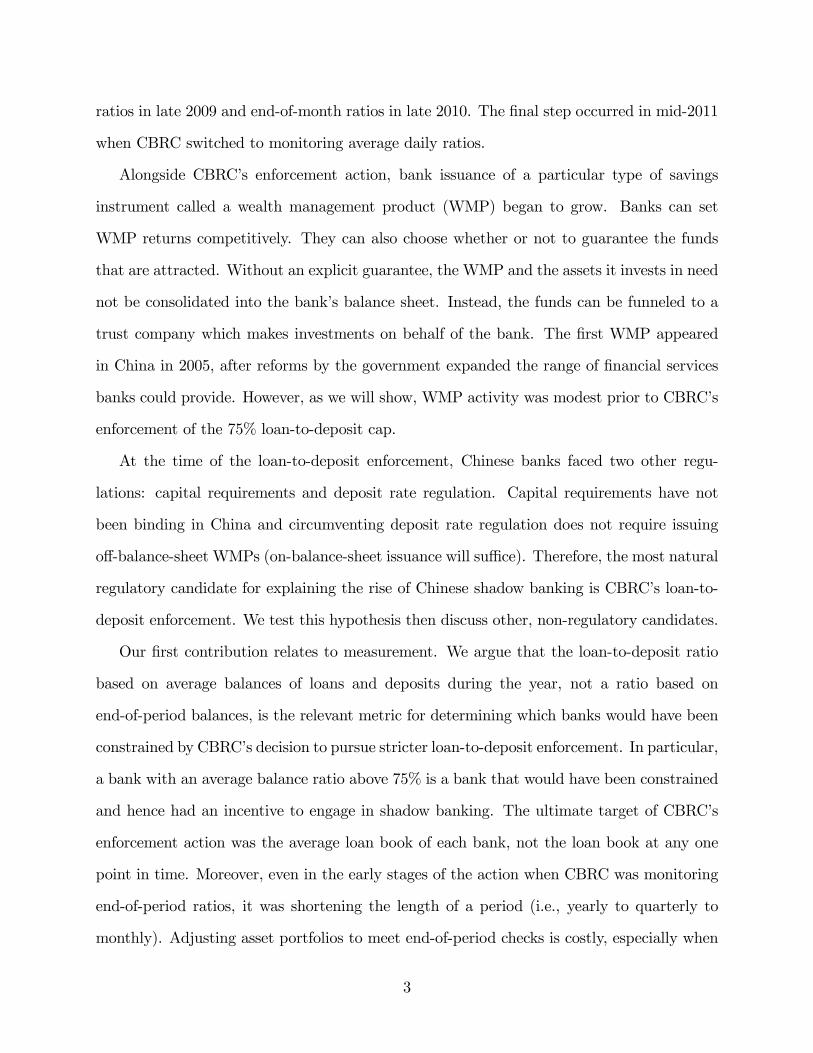
Figure 1 plots the evolution of WMPs in China after these products became legal in
2005. There is a near lockstep evolution of trust company assets under management and
WMPs outstanding. According to CBRC, non-guaranteed products were 70% of total WMP
issuance in 2012 and 65% of total WMP issuance in 2013. The proportion of non-guaranteed
WMPs is therefore very similar to the proportion of trust capital already pooled together by
other institutions (70% as cited above using CTA data). Given that trust company assets
under management line up almost exactly with WMPs outstanding (Figure 1), the similarity
in proportions also translates into a similarity in RMB value.
Further evidence that trust companies are major recipients of WMP money comes from
the fact that they have responded to attempts at WMP regulation. For example, in August
2010, CBRC announced that WMPs could invest at most 30% in trust loans. The composi-
tion of trust assets as reported by CTA then changed from 63% loans at the end of 2010Q2
to 42% loans by the end of 2011Q3, with “long-term investments”replacing loans.
On average, 70% of trust assets took the form of loans or long-term investments from
2010 to 2014. The long-term nature of trust company assets is also apparent from the fact
that trusts issued products with an average maturity of 1.7 years when trying to pool money
on their own during the first half of 2013.2 In contrast, WMPs are short-term products.
2Annual Report of the Trust Industry in China (2013).
10
Based on data from Wind Financial Terminal, the median maturity has been between 2 and
4 months since 2008, with roughly 25% of WMPs issued at a maturity of 1 month or less.
The funneling of WMP money to trust companies thus involves a maturity mismatch.
The non-guaranteed WMPs at the heart of bank-trust cooperation are therefore shadow
banking. First, they involve maturity transformation and thus constitute banking in the
sense of Diamond and Dybvig (1983). Second, they are booked off-balance-sheet and away
from regulatory standards.
3.2 Sizing the Shadow Sector
Based on the above discussion, we can use non-guaranteed WMPs to get a conservative
estimate of the size of China’s shadow banking system. Notice from Figure 1 that WMP
activity was modest prior to 2008, with WMPs outstanding amounting to less than 2% of
GDP in 2006 and 2007. In contrast, the period after 2008 was characterized by rapid growth
of WMPs and, by 2014, the amount outstanding stood at nearly 25% of GDP. Also recall
that roughly two-thirds of WMP issuance in 2012 and 2013 was non-guaranteed (CBRC).
We thus estimate that China’s shadow banking system grew from a negligible fraction of
GDP in 2007 to 16% of GDP in 2014.
To get a broader estimate of shadow banking, one can use the widely-cited data on
total social financing constructed by China’s National Bureau of Statistics (NBS). Social
financing includes bank loans, corporate bonds, equity, and other financing not accounted for
by traditional channels. Roughly one-third of other financing takes the form of undiscounted
banker’s acceptances.3 Removing these acceptances then leaves the most shadowy part of
other financing, namely loans by trust companies and firm-to-firm loans that use banks as
trustees (entrusted loans). The NBS defines trust loans very narrowly so credit extended
by trust companies in more obscure ways may actually be picked up in entrusted lending.
3A banker’s acceptance is basically a guarantee by a bank on behalf of a depositor. More precisely, thebank guarantees that the depositor will repay a third-party at a later date.
11
To this point, Allen, Qian, Tu, and Yu (2015) find that firms which are required to disclose
entrusted loans (in particular, publicly traded firms) accounted for 10% of total entrusted
lending reported by China’s central bank in 2013. In other words, the set of entrusted loans
for which it is easiest to identify and exclude trust company involvement accounts for only a
small fraction of entrusted lending. If trust and entrusted loans are grouped into one measure
of shadow banking, then shadow banking grew from 5% of GDP in 2007 to 24% of GDP in
2014. This 19 percentage point increase is similar to the approximately 15 percentage point
increase estimated above using only off-balance-sheet WMPs.
4 Liquidity Regulation as the Trigger
What accounts for the timing of shadow banking in China? WMPs became legal in the mid
2000s but they did not begin to take off until the late 2000s. Given that shadow banking
skirts regulation, the natural place to look is regulatory changes in the late 2000s.
Section 2.2 outlined a material change in liquidity regulation around 2008, as CBRC
moved to enforce the 75% loan-to-deposit cap. We also established that capital requirements
have not been binding in China and that circumventing deposit rate regulation does not
require issuing off-balance-sheet WMPs (on-balance-sheet issuance will suffi ce, as we will
discuss further in Section 5.1). The most natural candidate for explaining shadow banking
as regulatory arbitrage is therefore CBRC’s loan-to-deposit enforcement.
We test this explanation here. Section 4.1 sketches a simple theoretical model to motivate
the use of cross-sectional heterogeneity in our empirical tests. Section 4.2 then turns to the
data, establishing and exploiting cross-sectional differences in the bindingness of the 75% cap
to show that shadow banking in China emerged as a response to stricter liquidity regulation.
The importance of loan-to-deposit rules is also evidenced in Section 4.3, where we present
a detailed case study that shows changes in off-balance-sheet WMP characteristics are well
explained by changes in CBRC’s monitoring frequency.
12
4.1 A Simple Theoretical Model
If loan-to-deposit regulation triggered the rise of shadow banking in China, we should see
more shadow banking activities among banks that were more constrained by the regulation.
We formalize this idea here, before taking it to the data.
4.1.1 Environment
There are three periods, t ∈ {0, 1, 2}, and a continuum of risk neutral banks j ∈ [0, 1]
distributed uniformly over the unit interval. Bank j has access to a long-term investment
project with rate of return rj between t = 0 and t = 2. Without loss of generality, there is
a j0 ∈ [0, 1) such that rj = r0 for all j ∈ [0, j0] and rj > ri for all i, j ∈ [j0, 1] where j > i.
Projects cannot be liquidated at t = 1 (formally, the rate of return between t = 0 and t = 1
is −1), nor can additional investments be made at t = 1.
Banks have to attract funding from ex ante identical households who cannot directly
access projects. To this end, bank j offers a financial product with rate of return 0 between
t = 0 and t = 1 and rate of return ξj ≥ 0 between t = 0 and t = 2. The preferences of
households are such that they value the ability to liquidate at t = 1, hence why bank j does
not set the rate of return between t = 0 and t = 1 to −1. Diamond and Dybvig (1983)
provide the seminal treatment of these issues so we just take as given that banks provide a
liquidity service.
To study shadow banking, we introduce off-balance-sheet vehicles. Let X(ξj)denote the
savings that bank j attracts at t = 0 by offering a liquidity service with ξj. To fix ideas,
we use the demand function X(ξj)
= ϕξj, where ϕ > 0. Intuitively, bank j will get more
funding if it offers a higher return ξj. We then model that bank j can move an amount
Sj ∈[0, X
(ξj)]of its funding to an off-balance-sheet vehicle at a quadratic cost γ
2S2j , where
γ > 0. Effectively, bank j pays a cost to set up a separate company with a separate balance
sheet. The true financial position of bank j is represented by the sum of the two balance
sheets but they are legally distinct balance sheets when it comes to regulatory reporting.
13
The amount of funding that bank j invests in the long-term project, either directly or
through the separate company, is X(ξj)− Rj, where Rj denotes reserves that can be used
to satisfy household liquidations at t = 1. The fraction of households that liquidate savings
from each bank at t = 1 is θ ∈ (0, 1). The profit of bank j at the end of t = 2 is then:
Πj = (1 + rj)(X(ξj)−Rj
)+ (1 + iL)
(Rj − θX
(ξj))
(1)
− (1− θ)(1 + ξj
)X(ξj)− γ
2S2j
where iL is an interest rate at which banks can borrow and lend reserves at t = 1. All banks
take iL as given but, to close the model, iL is pinned down by:
iL = δ
∫ (θX(ξj)−Rj
)dj (2)
where δ > 0. In words, there is an external source of liquidity (e.g., the central bank) whose
supply of reserves, 1δiL, is increasing in the interest rate iL. The value of iL in equation (2)
implies zero net demand for reserves at t = 1.
4.1.2 Effect of Liquidity Regulation
Suppose the government announces that bank reserves as a fraction of bank funding must
exceed some floor α ∈ (0, 1) at t = 0. Only bank balance sheets are within the purview of
the regulation so each bank j must satisfy:
Rj ≥ α(X(ξj)− Sj
)(3)
Implicit in (3) is the idea that bank j records all of its reserves Rj on its own balance
sheet, even if it moves some of its funding to a separate company. This is optimal given
γ > 0: bank j has no incentive to pay for a separate balance sheet if its own balance sheet is
unconstrained by (3) so the allocation that satisfies (3) at minimum cost keeps all reserves
14
on the bank’s own balance sheet. The only assets held in the off-balance-sheet vehicle are
therefore long-term investments in the amount of the off-balance-sheet funding Sj.
Bank j chooses ξj ≥ 0, Sj ∈[0, X
(ξj)], and Rj at t = 0 to maximize Πj as defined in
(1) subject to the liquidity regulation in (3). The first order condition with respect to Rj is:
λj = rj − iL (4)
where λj is the Lagrange multiplier on (3). This multiplier measures the shadow cost to
bank j of holding reserves. A bank with λj > 0 would like to invest all of its funding in the
long-term project to earn rj at t = 2, honoring household liquidations in t = 1 by borrowing
reserves at the interest rate iL. The higher is λj at the optimal solution, the more constrained
is bank j by the liquidity regulation. In contrast, a bank with λj = 0 is indifferent between
holding reserves and investing in the long-term project, making it unconstrained by the
liquidity regulation.
The following proposition, proven in Appendix A, shows that more constrained banks
engage in more shadow banking:
Proposition 1 Fix α > 0 and focus on parameters that deliver an equilibrium with iL > 0.
Such parameters exist and, for any combination of them, the equilibrium has Sj′ > Sj for any
j and j′ such that λj′ > λj. Moreover,Sj′
X(ξj′)≥ Sj
X(ξj)with equality if and only if Sj
X(ξj)= 1.
In the simple model presented here, cross-sectional differences in the bindingness λj of the
liquidity regulation stem from cross-sectional differences in the long-term project returns rj.
Returning to (4), the least constrained banks are the ones with the lowest rj and, as verified
in Appendix A, any bank j ∈ [0, j0] is actually unconstrained when α and 1δare not too
high (i.e., the regulation is not exorbitant and external liquidity is not very responsive to
the interest rate iL).
Heterogeneity in rj is a parsimonious way of modeling heterogeneity among banks. In
Hachem and Song (2017), we showed that a crucial dimension on which China’s banks differ
15
is interbank market power. In particular, the Big Four are large enough to be interbank
price-setters while other Chinese banks, such as the JSCBs, are individually much smaller
and hence behave more like interbank price-takers. We also showed that interbank price-
setters, by virtue of internalizing how their reserve decisions affect liquidity on the interbank
market, choose higher liquidity ratios than interbank price-takers. The price-setters are
therefore less constrained by the introduction of a liquidity floor, but they also utilize their
price impact in a game of asymmetric competition that helps generate an unintended credit
boom.
The model in Hachem and Song (2017) has deeper microfoundations than we need to
motivate the empirical tests below so Proposition 1 was derived by just assuming that banks
differ on rj. However, it is useful to point out that the intuition behind (4) transcends the
specific assumption used here. Equation (4) says that the extent to which liquidity regulation
constrains bank j depends on how bank j perceives the return from its long-term project
relative to the return from lending reserves at t = 1. Interbank price-setters can strategically
use the interbank market to extract rents so, loosely speaking, they can be interpreted as
perceiving a relative return from long-term projects that is lower than the relative return
perceived by interbank price-takers. Under this interpretation, the price-setters would be
the lower λj banks in the model we have presented here.
4.2 Cross-Sectional Evidence
To construct a test based on Proposition 1, we need a measure of how constrained a bank
is. We argue that loan-to-deposit ratios based on average balances during the year provide
a reasonable indication in the early stages of CBRC’s enforcement action. Average balance
data is tabulated in the net interest analysis of bank annual reports, not the standard balance
sheets that appear at the end of these reports.
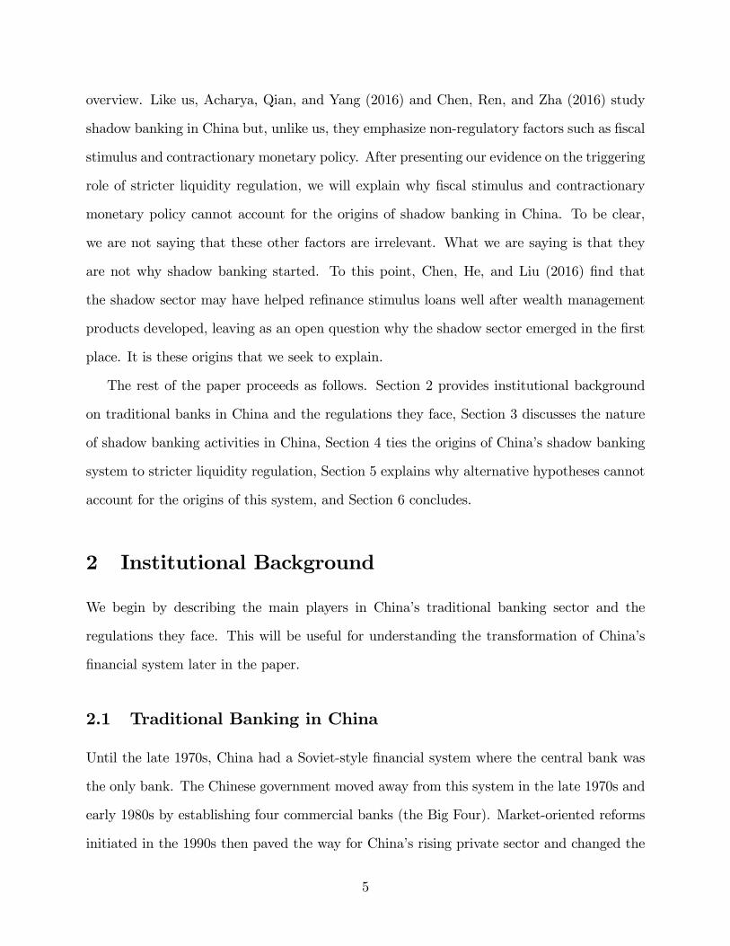
Figure 2 compares loan-to-deposit ratios based on average balance data (dashed lines)
to those based on end-of-year data (solid lines). We plot ratios for the Big Four (blue)
16
and the JSCBs (red) from 2005 to 2014. Historical data for city and rural banks is spotty,
particularly when it comes to average balances, so these banks are excluded from the figure.4
There are two salient differences between the Big Four and the JSCBs in Figure 2. First,
there has never been a sizeable difference between the average balance and year-end loan-to-
deposit ratios of the Big Four. In contrast, the JSCBs had consistently higher average balance
ratios than year-end ratios prior to 2012, the first full year of average balance monitoring by
CBRC. Second, the Big Four had both ratios comfortably below 75% before CBRC heralded
the era of stricter and more frequent loan-to-deposit enforcement in 2008. This was not the
case for the JSCBs who, as a group, were well above 75% based on average balance data and
very close to 75% based on year-end data.5
Banks whose loan-to-deposit ratios are materially lower at the end of the year than on an
average day during the year are window-dressing their year-end balance sheets. As discussed
in Section 2.2, the 75% cap was legislated in 1995 and subject to occasional inspection before
CBRC’s enforcement action. Among banks with high loan-to-deposit ratios, a common
practice in China prior to 2008 was to call loans shortly ahead of a potential inspection (e.g.,
the end of a calendar year). The bank promises borrowers whose loans are called that it will
re-issue the loans within a few weeks and, in the intervening time, the borrowers rely on loan
sharks. Called loans are therefore erased from the bank’s balance sheet at year-end, but not
during the rest of the year.
A bank that was window-dressing its year-end balance sheet before 2008 is a bank that
would have become constrained as CBRC transitioned towards monitoring average balance
ratios, ceteris paribus. Borrowers cannot afford to rely increasingly on price-gouging loan
sharks so the practice of calling loans is only a viable option for reducing loan-to-deposit
ratios if it does not have to occur frequently. Window-dressing banks therefore needed to find
4One JSCB (Evergrowing Bank) is also excluded for similar reasons.5Figure 2 also shows that the loan-to-deposit ratio of the Big Four has increased towards 75% since the
beginning of the enforcement. In Hachem and Song (2017), we demonstrate that much of this increase canbe explained as a strategic response to increased competition from shadow banking.
17
another practice when CBRC announced in 2008 that it would be moving towards stricter
and more frequent loan-to-deposit enforcement.
If CBRC’s enforcement action triggered shadow banking in China, the JSCBs should
have moved more heavily into non-guaranteed WMPs than the Big Four: Figure 2 provides
strong evidence that the JSCBs would have been more constrained by the regulation and
Proposition 1 predicts that more constrained banks engage in more shadow banking. Data
from Wind corroborate this. Between 2008 and 2014, the JSCBs accounted for 73% of all
newWMP batches and issued 57% of their batches without a guarantee. The Big Four issued
only 46% of their batches in this way. The gap in non-guaranteed intensity widens in the
second half of the sample, with the JSCBs at 62% and the Big Four at 43%. These estimates
are based on product counts since Wind does not yet have complete data on the total funds
raised by each product. However, using data from CBRC and the annual reports of the Big
Four, we estimate that small and medium-sized banks (i.e., JSCBs and smaller) accounted
for roughly 64% of non-guaranteed WMP balances outstanding at the end of 2013.6 This
conveys a consistent message with the batch statistics.
To provide more formal and disaggregated evidence, we run panel regressions in Table
1. We use bank-level data for each bank in the Big Four and the JSCBs. The dependent
variable is the log of non-guaranteed WMP batches issued by bank i in year t scaled by the
average balance of deposits at the bank in that year. The main sample covers 2008 to 2010
inclusive. Recall that CBRC reached its final goal of average balance monitoring in mid-2011,
making 2010 the last full year in which average balance ratios exhibit meaningful variation
among constrained banks.7 In the first column of Table 1, we regress the dependent variable
6The entire WMP balance in Bank of China’s annual report is described in the notes as an unconsolidatedbalance yet the micro data in Wind includes several guaranteed batches for this bank that would not havematured by the end of 2013. We therefore remove Bank of China and rescale the other banks in the BigFour to back out our 64% estimate for small and medium-sized banks.
7We can see this from the model in Section 4.1. All bank balance sheets satisfy (3) and λj ≥ 0 withcomplementary slackness. Therefore, at the frequency monitored by the regulator, the econometrician willobserve a loan-to-deposit ratio of 1 − α for any constrained bank (λj > 0) even though not all constrainedbanks have the same λj .
18
on the loan-to-deposit ratio of bank i in year t, as measured using average balance data.8 All
columns include year fixed effects. We also control for the maturity of the non-guaranteed
WMPs issued by bank i in year t. A bank that issues 3-month WMPs will issue twice as
many WMP batches as a bank that issues 6-month WMPs to raise the same amount of
funding over the course of a year. The bank with shorter-term WMPs will therefore have
more batches, even if it is otherwise identical to the bank with longer-termWMPs. Including
maturity as a regressor controls for this.
The results in the first column of Table 1 confirm that banks with higher average balance
ratios issued more non-guaranteed WMPs than banks with lower ratios. The second column
shows that this finding is robust to controlling for the average return floor advertised by
bank i when issuing non-guaranteed WMPs in year t. The third column shows that it is
also robust to including bank fixed effects. In the fourth column, we extend the sample
to 2014. The coeffi cient on the average balance ratio is still positive but its magnitude is
roughly one-third of the magnitudes in the columns based on the main sample, and it is only
statistically significant at the 10% level. The extended sample gives us more observations,
and hence more degrees of freedom, to include the bank fixed effects. However, as noted
earlier, the average balance ratio becomes a truncated indicator after 2010.
In the last two columns of Table 1, we rerun the main sample regressions with the average
balance ratio decomposed into two components: the regulated ratio of bank i in year t, as
measured at the end of the year, and the degree of window-dressing by bank i in year t, as
measured by the percent difference between the bank’s average balance and regulated ratios.9
The degree of window-dressing is the indication of constraint in this decomposition. The
results in the last two columns corroborate what we found earlier: banks more constrained by
8One may worry about reverse causality here. Specifically, the average balance ratio will decrease as thebank issues non-guaranteed WMPs to move some business off-balance-sheet. However, this implies a negativerelationship between the dependent variable and the average balance ratio, which will bias the regressionagainst us.
9We have to focus on the main sample in these columns as this is the sample where window-dressingis an observable (i.e., the average balance ratio becomes the regulated ratio once CBRC begins monitoringaverage balance ratios).
19
CBRC’s impending monitoring of average balance ratios issued more non-guaranteed WMPs
than banks less constrained.
4.2.1 Additional Tests
In Table 2, we conduct Granger causality tests on total WMP issuance and find that the
WMPs issued by the Big Four were a response to the WMP activities of small and medium-
sized banks (SMBs). We use differenced monthly data on WMP batches between January
2008 and September 2014 to run the tests. The Akaike Information Criterion (AIC) selects
a VAR with 21 lags. As shown in Table 2, the null hypothesis that WMP issuance by SMBs
does not Granger-cause WMP issuance by the Big Four is rejected at 1% significance. The
opposite hypothesis that WMP issuance by the Big Four does not Granger-cause WMP
issuance by SMBs cannot be rejected at any reasonable level of significance. Using the
Bayesian Information Criterion (BIC) to select the number of lags yields similar results, as
do Granger causality tests based on other orders. The impetus for WMP activity in China
is therefore coming from the SMBs, who are also the constrained banks and the banks more
heavily involved in non-guaranteed issuance.
Even though the Big Four ultimately responded to the WMP activities of SMBs by
issuing their own products, the products they issued were still less aggressive than those of
the SMBs. The first column in Table 3 shows that the realized returns on WMPs issued
by the Big Four were on average 24 basis points lower than the realized returns on WMPs
issued by SMBs. The regression uses product-level data from 2008 to 2014, includes time
dummies, and controls for WMP maturity. The second and third columns of Table 3 then
show that realized returns relative to the expected floors and ceilings advertised at issuance
were higher for Big Four WMPs than for the WMPs issued by SMBs. Taken together with
the first column, this suggests that the Big Four were also more conservative in the range
of returns they advertised to investors, with ceilings and floors respectively averaging 29
and 110 basis points below those advertised by SMBs. With small and medium-sized banks
20
offering notably more aggressive returns than large banks, it becomes clearer why the Big
Four experienced the post-restructuring decline in market share discussed at the end of
Section 2.1.
4.3 Case Study Evidence
A detailed case study will shed further light on the motives that drive small and medium-
sized banks. We consider China Merchants Bank (CMB), one of the twelve JSCBs. Between
2007 and 2013, CMB’s loan-to-deposit ratio averaged 82% when calculated using average
balances during the year. This is in contrast to 74% when end-of-year balances are used.
WMP issuance by CMB increased from RMB 0.1 trillion in 2007 to RMB 0.7 trillion in
2008 before reaching almost RMB 5 trillion in 2013. CMB accounted for only 3% of total
banking assets in 2012 but 5.2% of WMPs outstanding at year-end and 17.7% of all WMPs
issued during the year.10 At the end of both 2012 and 2013, CMB had about 83% of its
outstanding WMP balances booked off-balance-sheet and, based on notes to the financial
statements, figures for earlier years were at least as high.
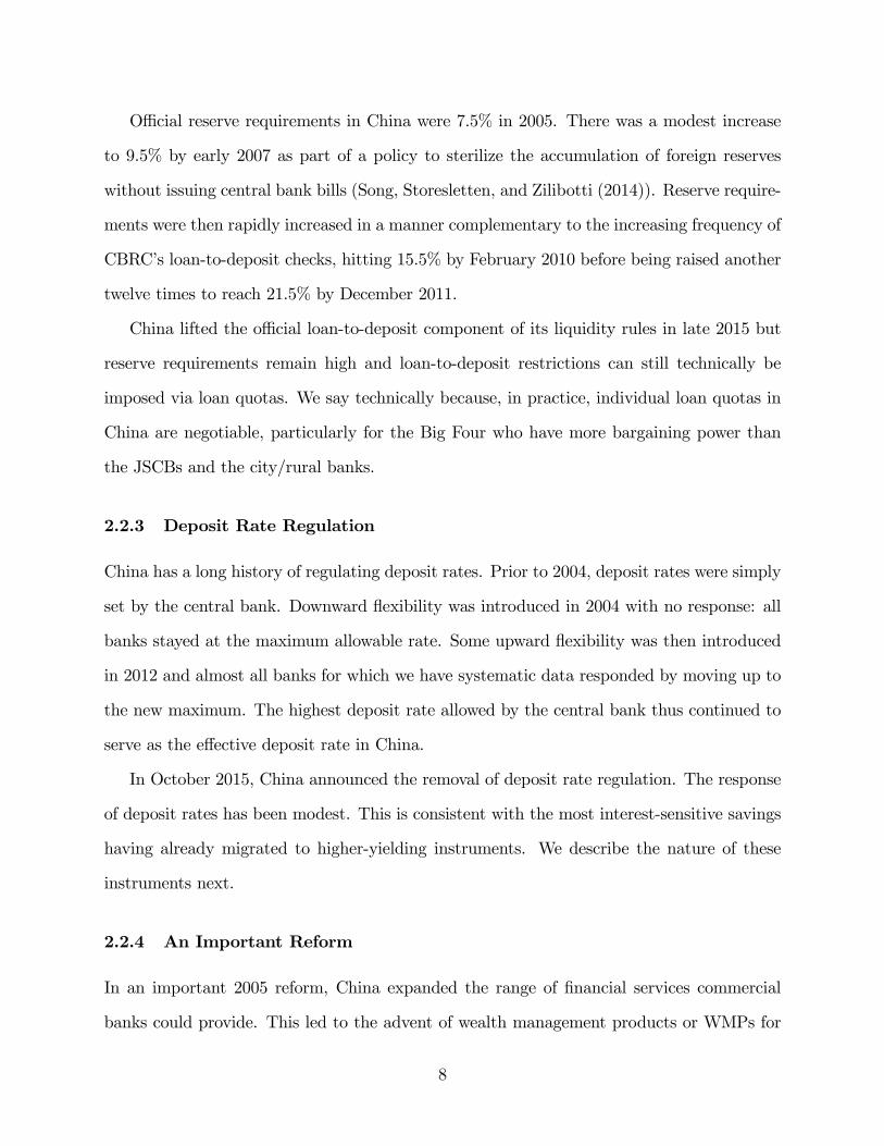
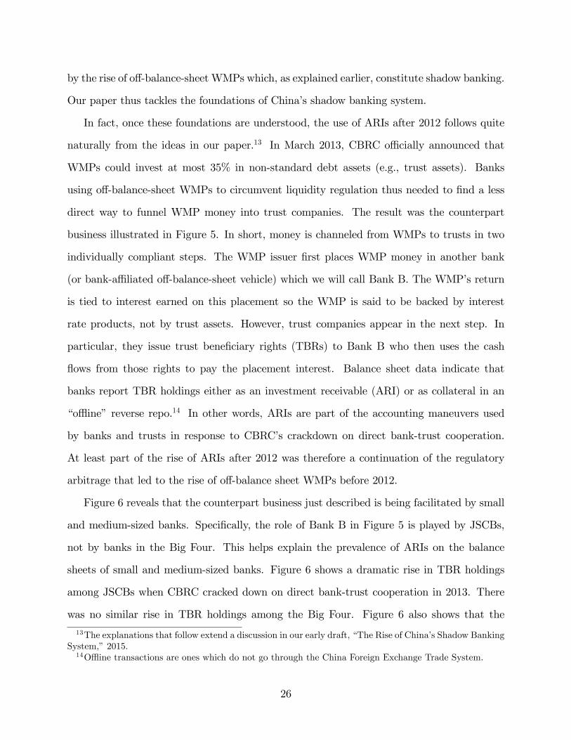
We argue that time variation in the maturity of CMB’s off-balance-sheet WMPs reveals
the importance of loan-to-deposit regulation for the evolution of these products. Figure 3
shows a sizeable drop in the median maturity of CMB’s off-balance-sheet products, from
just over 4 months in late 2009 to just under 1 month by mid-2011. Figure 3 also shows
that this drop does not occur for on-balance-sheet WMPs nor is it matched by a drop in the
advertised yield on off-balance-sheet products. Instead, the drop in CMB’s off-balance-sheet
maturity coincides with changes in the frequency of CBRC’s monitoring of loan-to-deposit
ratios. Recall from Section 2.2 that CBRC focused on the end-of-year ratio until late 2009,
the end-of-quarter ratio until late 2010, and the end-of-month ratio until mid-2011. CMB
thus shortened the maturity of its off-balance-sheet products as the frequency of CBRC
exams increased.10Based on data from KPMG, CBRC, and China Merchants Bank.
21
This is significant because shorter maturities can be used to thwart more frequent end-
of-period exams. Upon maturity, the principal and interest from an off-balance-sheet WMP
are automatically transferred to the buyer’s deposit account. A buyer who wants to roll over
his investment then contacts his bank to have the transfer reversed. In the time between
the transfer and the reversal though, reserves and deposits rise, lowering the loan-to-deposit
ratio observed by CBRC.11 In the first half of 2011, CMB’s off-balance-sheet products had
a median maturity of just under 1 month, which enables the transfers that thwart end-
of-month exams. To make this point more concrete, we can look at the maturity of each
off-balance-sheet batch relative to its issue date in Wind. Approximately 15% of the off-
balance-sheet batches issued by CMB between January 2008 and December 2010 would have
matured near a month-end. This fraction jumped to 40% in early 2011.
Shortening the maturity of off-balance-sheet WMPs in response to increasingly frequent
monitoring of end-of-period loan-to-deposit ratios became futile in mid-2011 as CBRC began
monitoring average daily ratios, not end-of-period ratios. Accordingly, Figure 3 shows that
CMB’s median off-balance-sheet maturity has returned to roughly 3 months. The fraction
of off-balance-sheet batches set to mature near a month-end has also fallen back below 20%.
Similar patterns are not observed for the Big Four. That is, changes in WMP maturity do
not track changes in the frequency of CBRC’s monitoring of loan-to-deposit rules when we
restrict attention to WMPs issued by banks in the Big Four.
5 Robustness to Alternatives
Our headline result is that stricter liquidity regulation triggered the rise of China’s shadow
banking system. Other factors may have amplified the growth of the shadow sector after
it emerged but the origins of the system lie in circumvention of CBRC’s liquidity rules. In
11Keeping the automatic deposits as reserves is one approach. Another is to bring loans back on balancesheet in the form of securities which derive their cash flows from the loans. The data suggest that CMB justrecorded reserves between 2009 and 2011.
22
this section, we discuss alternative hypotheses for the rise of shadow banking in China and
explain why these hypotheses cannot account for the origins of the system.
5.1 Fiscal Stimulus and Shadow Banking
China’s State Council announced a two-year fiscal stimulus package in late 2008 which would
have created roughly RMB 4 trillion of new investment opportunities for the banking sector
to fund. Acharya, Qian, and Yang (2016) contend that fiscal stimulus increased the loan-to-
deposit ratios of small and medium-sized banks. The authors argue that Bank of China (one
of the Big Four) was particularly willing to provide stimulus loans and, as it raised deposits in
order to make these loans, its smaller competitors were crowded out of the deposit market and
forced to attract funding by issuing off-balance-sheet WMPs with high returns. This story
does not pose a challenge to our view that CBRC’s loan-to-deposit enforcement triggered
the rise of off-balance-sheet WMPs by small and medium-sized banks.
First, had CBRC not begun stricter enforcement of the loan-to-deposit cap, small and
medium-sized banks crowded out because of stimulus could have simply issued high-return
on-balance-sheet WMPs to attract funding and continue lending. As long as the WMP was
not classified as a traditional deposit, it would not have been subject to the central bank’s
deposit rate regulations. To this point, the return on 3-month on-balance-sheet WMPs
averaged almost 90 basis points above the 3-month benchmark deposit rate from 2008 to
2014, with the spread widening to over 130 basis points in the second half of this sample.
Second, stimulus-related forces are not the main reason why small and medium-sized
banks had high loan-to-deposit ratios around the time CBRC toughened its stance on the
75% cap. The stimulus package was announced in late 2008 and funded from 2009 to 2010
so, if stimulus explains why small and medium-sized banks were constrained by the 75%
loan-to-deposit cap, small and medium-sized banks should have had loan-to-deposit ratios
no higher than 75% in 2007 and 2008. The solid red line in Figure 2 shows that, as a group,
the JSCBs had a year-end ratio of 75% in both 2007 and 2008. One might then be tempted
23
to conclude that the JSCBs were already compliant with the 75% cap and that CBRC’s
enforcement action would have been irrelevant absent a shock that pushed the JSCB ratio
above 75%. This conclusion would be wrong. The JSCBs were not already compliant. As
explained in Section 2.2, stricter enforcement by CBRC involved an increase in monitoring
frequency to target average balance ratios. The dashed red line in Figure 2 shows that the
loan-to-deposit ratio of the JSCBs was around 85% in both 2007 and 2008 when the ratio
is calculated using average balances during the year. Increasingly strict enforcement of the
75% cap by CBRC would have therefore bound on these banks even without any additional
pressure from the stimulus package. This point underscores the importance of using average
balances during the year, not end-of-year balances, when calculating loan-to-deposit ratios
on the eve of the enforcement.
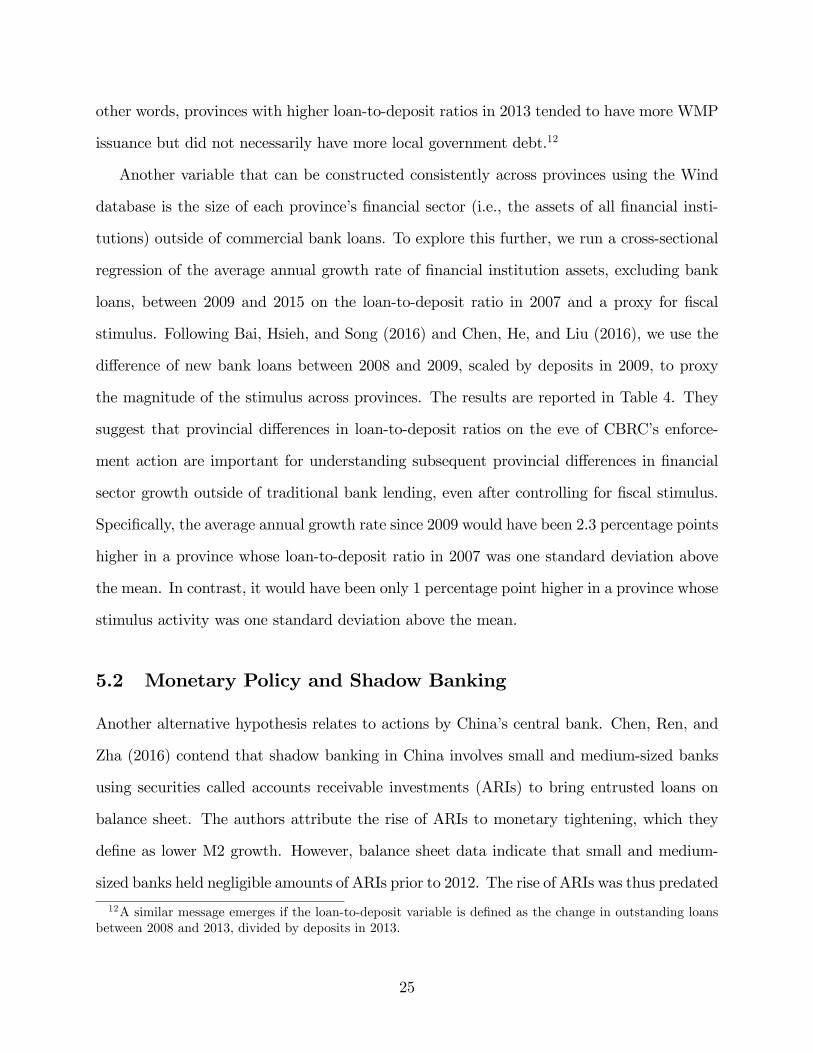
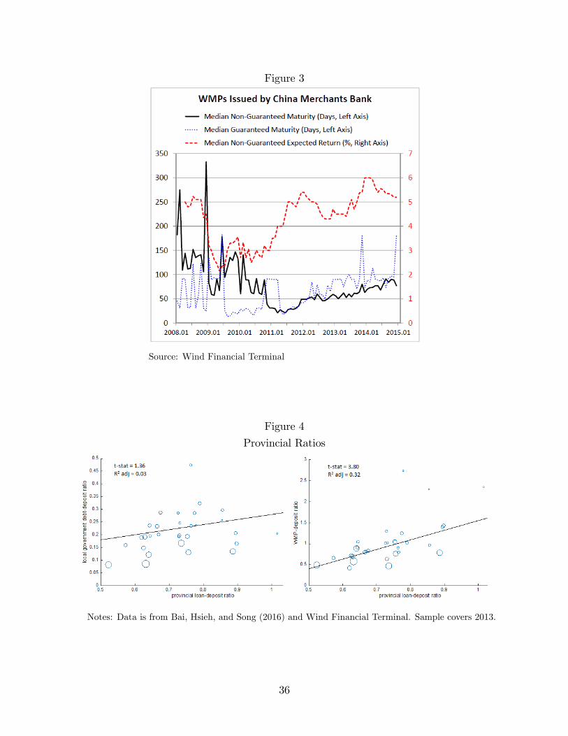
Third, when stimulus activity is measured using data from the borrowers, provinces
with the most stimulus activity were not necessarily those with the highest loan-to-deposit
ratios. As documented in Bai, Hsieh, and Song (2016), most of the stimulus package had
to be borrowed by local governments so it will be instructive to look specifically at local
government debt. For each province in 2013, the left panel of Figure 4 plots the stock
of local government debt (as a fraction of deposits) against the provincial loan-to-deposit
ratio. Regional data on loans and deposits comes from Wind and is based on aggregation
of bank branches by province. Bigger provinces, as measured by deposits, are represented
by bigger circles in Figure 4. For comparison, the right panel plots WMP batches (relative
to deposits in trillions of RMB) against loan-to-deposit ratios. CBRC enforced the 75%
cap at the bank level, not the branch level, so a distribution of provincial loan-to-deposit
ratios exists. However, individual branches would still have needed an infrastructure that
could accommodate sudden requests from their parent banks to decrease on-balance-sheet
loan-to-deposit ratios as the parents worked around CBRC’s enforcement, leaning against
different branches at different times. The positive correlation in the right panel of Figure
4 is statistically significant whereas the positive correlation in the left panel is not. In
24
other words, provinces with higher loan-to-deposit ratios in 2013 tended to have more WMP
issuance but did not necessarily have more local government debt.12
Another variable that can be constructed consistently across provinces using the Wind
database is the size of each province’s financial sector (i.e., the assets of all financial insti-
tutions) outside of commercial bank loans. To explore this further, we run a cross-sectional
regression of the average annual growth rate of financial institution assets, excluding bank
loans, between 2009 and 2015 on the loan-to-deposit ratio in 2007 and a proxy for fiscal
stimulus. Following Bai, Hsieh, and Song (2016) and Chen, He, and Liu (2016), we use the
difference of new bank loans between 2008 and 2009, scaled by deposits in 2009, to proxy
the magnitude of the stimulus across provinces. The results are reported in Table 4. They
suggest that provincial differences in loan-to-deposit ratios on the eve of CBRC’s enforce-
ment action are important for understanding subsequent provincial differences in financial
sector growth outside of traditional bank lending, even after controlling for fiscal stimulus.
Specifically, the average annual growth rate since 2009 would have been 2.3 percentage points
higher in a province whose loan-to-deposit ratio in 2007 was one standard deviation above
the mean. In contrast, it would have been only 1 percentage point higher in a province whose
stimulus activity was one standard deviation above the mean.
5.2 Monetary Policy and Shadow Banking
Another alternative hypothesis relates to actions by China’s central bank. Chen, Ren, and
Zha (2016) contend that shadow banking in China involves small and medium-sized banks
using securities called accounts receivable investments (ARIs) to bring entrusted loans on
balance sheet. The authors attribute the rise of ARIs to monetary tightening, which they
define as lower M2 growth. However, balance sheet data indicate that small and medium-
sized banks held negligible amounts of ARIs prior to 2012. The rise of ARIs was thus predated
12A similar message emerges if the loan-to-deposit variable is defined as the change in outstanding loansbetween 2008 and 2013, divided by deposits in 2013.
25
by the rise of off-balance-sheet WMPs which, as explained earlier, constitute shadow banking.
Our paper thus tackles the foundations of China’s shadow banking system.
In fact, once these foundations are understood, the use of ARIs after 2012 follows quite
naturally from the ideas in our paper.13 In March 2013, CBRC offi cially announced that
WMPs could invest at most 35% in non-standard debt assets (e.g., trust assets). Banks
using off-balance-sheet WMPs to circumvent liquidity regulation thus needed to find a less
direct way to funnel WMP money into trust companies. The result was the counterpart
business illustrated in Figure 5. In short, money is channeled from WMPs to trusts in two
individually compliant steps. The WMP issuer first places WMP money in another bank
(or bank-affi liated off-balance-sheet vehicle) which we will call Bank B. The WMP’s return
is tied to interest earned on this placement so the WMP is said to be backed by interest
rate products, not by trust assets. However, trust companies appear in the next step. In
particular, they issue trust beneficiary rights (TBRs) to Bank B who then uses the cash
flows from those rights to pay the placement interest. Balance sheet data indicate that
banks report TBR holdings either as an investment receivable (ARI) or as collateral in an
“offl ine” reverse repo.14 In other words, ARIs are part of the accounting maneuvers used
by banks and trusts in response to CBRC’s crackdown on direct bank-trust cooperation.
At least part of the rise of ARIs after 2012 was therefore a continuation of the regulatory
arbitrage that led to the rise of off-balance sheet WMPs before 2012.
Figure 6 reveals that the counterpart business just described is being facilitated by small
and medium-sized banks. Specifically, the role of Bank B in Figure 5 is played by JSCBs,
not by banks in the Big Four. This helps explain the prevalence of ARIs on the balance
sheets of small and medium-sized banks. Figure 6 shows a dramatic rise in TBR holdings
among JSCBs when CBRC cracked down on direct bank-trust cooperation in 2013. There
was no similar rise in TBR holdings among the Big Four. Figure 6 also shows that the
13The explanations that follow extend a discussion in our early draft, “The Rise of China’s Shadow BankingSystem,”2015.14Offl ine transactions are ones which do not go through the China Foreign Exchange Trade System.
26
JSCBs accommodated their increase in TBR holdings by keeping fewer balances at banks
and other financial institutions (dashed black line). In other words, the JSCBs did not
sacrifice loans in order to hold TBRs. The JSCBs’ substitution away from balances at
banks is also visible in the blue bars in Figure 6: both the JSCBs and the Big Four have
experienced decreases in balances owed to banks. However, unlike the Big Four, the JSCBs
have attracted suffi ciently more balances from non-bank financial institutions (red bars).
Off-balance-sheet vehicles that hold non-guaranteed WMPs would be classified as non-bank
financial institutions. Effectively, the off-balance-sheet vehicle of one JSCB places money
with another JSCB. The other JSCB then uses returns from its TBR holdings to pay interest
on the placement. This is exactly the counterpart business illustrated in Figure 5. In
principle, even more counterpart business could be occurring between the vehicles themselves
(e.g., vehicles can hold TBRs and placements can occur between vehicles).
6 Conclusion
This paper has argued that China’s shadow banking system emerged as a response to stricter
liquidity rules in the late 2000s. Chinese regulators began toughening bank liquidity stan-
dards through increasingly strict enforcement of a 75% loan-to-deposit cap. We showed
that small and medium-sized banks were constrained by stricter enforcement of the 75%
cap whereas big banks were not. In the process, we demonstrated that stronger identifica-
tion is obtained by looking at average balance data instead of end-of-period data. We then
used cross-sectional heterogeneity in the bindingness of the cap to test the hypothesis that
China’s shadow sector grew out of stricter liquidity regulation. If loan-to-deposit enforce-
ment triggered the rise of shadow banking products in China, then small and medium-sized
banks should have been much more heavily involved in the issuance of these products than
big banks. We found exactly this. We also showed that the maturity of shadow banking
products was varied by small and medium-sized banks to make the most out of the imple-
27
mentation schedule for increasingly frequent monitoring of the 75% cap, providing further
evidence on the importance of this cap for understanding the evolution of shadow banking
products in China. We concluded by discussing alternative hypotheses for the rise of shadow
banking in China and explaining why they cannot account for the origins of the system.
28
References
Acharya, V., J. Qian, and Z. Yang. 2016. “In the Shadow of Banks: Wealth Management
Products and Issuing Banks’Risk in China.”Mimeo.
Allen, F., J. Qian, and M. Qian. 2005. “Law, Finance, and Economic Growth in China.”
Journal of Financial Economics, 77(1), pp. 57-116.
Allen, F., Y. Qian, G. Tu, and F. Yu. 2015. “Entrusted Loans: A Close Look at China’s
Shadow Banking System.”Mimeo.
Bai, C., C. Hsieh, and Z. Song. 2016. “The Long Shadow of a Fiscal Expansion.”Brookings
Papers on Economic Activity, Fall 2016.
Brandt, L., J. Van Biesebroeck, and Y. Zhang. 2012. “Creative Accounting or Creative
Destruction? Firm-Level Productivity Growth in Chinese Manufacturing.” Journal of
Development Economics, 97(2), pp. 339-351.
Chen, K., J. Ren, and T. Zha. 2016. “What We Learn from China’s Rising Shadow Banking:
Exploring the Nexus of Monetary Tightening and Banks’Role in Entrusted Lending.”
NBER Working Paper 21890.
Chen, Z., Z. He, and C. Liu. 2016. “The Financing of Local Government in China: Stimulus
Loan Wanes and Shadow Banking Waxes.”Mimeo.
Cheremukhin, A., M. Golosov, S. Guriev, and A. Tsyvinski. 2015. “The Economy of People’s
Republic of China from 1953.”NBER Working Paper No. 21397.
Diamond, D. and P. Dybvig. 1983. “Bank Runs, Deposit Insurance, and Liquidity.”Journal
of Political Economy, 91(3), pp. 401-419.
Elliott, D., A. Kroeber, and Y. Qiao. 2015. “Shadow Banking in China: A Primer.”Brookings
Year Dummies X X X X X XBank Dummies × × X X × XR-squared 0.583 0.654 0.965 0.793 0.658 0.963
Notes: The dependent variable is the log of the total number of non-guaranteed WMPs issued by a bank
in a year scaled by the average balance of deposits at the bank in that year. LDR is the loan-to-deposit
ratio based on average balances of a bank in a year. Maturity and MinROR are respectively the average
maturity and expected return floor on non-guaranteed WMPs issued by a bank in a year. WinDress is
the percent difference between the average balance and year-end loan-to-deposit ratios of a bank in a
year. RegRatio is the year-end ratio of a bank in a year. In all columns except (4), the sample period is
2008-2010. In column (4), the sample period is 2008-2014. Standard errors, clustered at the bank level,
are in parentheses. ***p<0.01, **p<0.05, *p<0.1
31
Table 2:
Granger Causality Tests
H0: SMB WMPs do not cause Big Four WMPs
Criteria Order F-statistic P-value
AIC 21 3.737 0.00
BIC 1 17.707 0.00
3 15.276 0.00
6 11.514 0.00
9 2.295 0.02
H0: Big Four WMPs do not cause SMB WMPs
Criteria Order F-statistic P-value
AIC 21 0.236 0.99
BIC 1 0.098 0.75
3 0.966 0.41
6 1.590 0.15
9 0.492 0.88
Notes: We use monthly differenced data on WMP batches. AIC is the
Akaike Information Criterion, which helps select the lag order of a VAR
model for the Granger tests. BIC is the Bayesian Information Criterion.
AIC usually over-estimates the order with positive probability, whereas
BIC estimates the order consistently under fairly general conditions.
Thus, BIC is typically used as the main selection criterion.
32
Table 3:
WMP Returns
realized r_gap_h r_gap_l
B4 -0.237*** 0.049*** 0.866***
(0.012) (0.013) (0.025)
Maturity 0.092*** -0.044*** -0.021***
(0.001) (0.002) (0.003)
Observations 54,294 52,090 34,876
Year Dummies X X XMonth Dummies X X XR-squared 0.293 0.069 0.090
Notes: “realized”is the realized WMP return, “r_gap_h”is the realized
return less the ceiling expected by the bank at issuance, “r_gap_l”is the
realized return less the floor expected by the bank at issuance. B4 is a
dummy for banks in the Big Four. Maturity is the maturity of the WMP.
Standard errors are in parentheses. ***p<0.01, **p<0.05, *p<0.1
33
Table 4:
Financial Sector Growth Excluding Bank Loans
(1) (2)
ldr_07 0.270*** 0.232***
(0.057) (0.059)
new_loan_diff_09 0.495*
(0.289)
Observations 30 30
R-squared 0.445 0.500
Notes: The dependent variable is the average annual growth rate of
all financial institution assets, excluding bank loans, in a province
between 2009 and 2015. “ldr_07”is the loan-to-deposit ratio in the
province in 2007. “new_loan_diff_09”is the difference of new bank
loans in the province between 2008 and 2009, scaled by deposits in
2009. Standard errors in parentheses. ***p<0.01, **p<0.05, *p<0.1
34
Figure 1
Source: PBOC, CBRC, IMF, China Trustee Association, KPMG China Trust Surveys
Figure 2
Notes: Data is from Bankscope and bank annual reports. Shaded area is interquartile range.
35
Figure 3
Source: Wind Financial Terminal
Figure 4
Provincial Ratios
Notes: Data is from Bai, Hsieh, and Song (2016) and Wind Financial Terminal. Sample covers 2013.
36
Figure 5
Business with Counterparts
Notes: TBR stands for trust beneficiary right; SPV is an off-balance-sheet vehicle
Figure 6
Notes: Data is from bank annual reports. The graphs report domestic balances only. TBR stands
for trust beneficiary right. FI stands for financial institution.
37
Appendix A
This appendix proves Proposition 1 in the main text.
As a Lagrange multiplier, λj in (4) must be non-negative for all j ∈ [0, 1]. Accordingly,
λ0 ≡ r0 − iL ≥ 0 and λj > 0 for all j ∈ (j0, 1].
The first order condition with respect to ξj is:
2 (1− θ) ξj = rj − θiL − αλj +υjϕ
+ η1j (5)
where υj ≥ 0 and η1j ≥ 0 are the Lagrange multipliers on ξj ≥ 0 and Sj ≤ X(ξj)respectively.
If υj > 0, then ξj = 0 and equation (5) implies rj − θiL−αλj < 0. Using (4), this inequality
becomes λj + 1−θ1−αiL < 0, which is impossible given λj ≥ 0 and iL > 0 as shown below.
Therefore, υj = 0 and ξj > 0.
The first order condition with respect to Sj is:
η1j − η0j = αλj − γSj (6)
where η0j ≥ 0 is the Lagrange multiplier on Sj ≥ 0. If η0j > 0, then Sj = 0 and (6) implies
η1j − η0j = αλj ≥ 0. This would require η1j > 0 and hence Sj = X(ξj), which violates Sj = 0
given X(ξj)
= ϕξj and ξj > 0 as shown above. Therefore, η0j = 0.
If η1j = 0, then (5) and (6) with υj = η0j = 0 become:
ξj =1
2
(iL +
1− α1− θ λj
)(7)
and:
Sj =α
γλj (8)
respectively, where we have used (4) to substitute rj out of (5). It is easy to see that Sj is
increasing in λj. We can also write:
Sj
X(ξj) =
2α
γϕ
λjiL + 1−α
1−θ λj
which is increasing in λj for iL > 0. To confirm η1j = 0, we need Sj ≤ X(ξj)or, equivalently:(
2α
γϕ− 1− α
1− θ
)λj ≤ iL (9)
38
Define:
α ≡ 1
1 + 2(1−θ)γϕ
If α ≤ α, then the left-hand side of (9) is non-positive so, with iL > 0, (9) always holds. If
instead α > α, then we can define a cutoff j1 ∈ [0, 1] such that (9) is satisfied if and only if
j < j1.
For cases where (9) does not hold (i.e., j > j1 when α > α), we have η1j > 0. Hence:
Sj = X(ξj)
and:
ξj =λj + (1− θ) iL2 (1− θ) + γϕ
from (5) and (6) with υj = η0j = 0 and rj substituted out using (4). Clearly, higher λjimplies higher ξj which in turn implies higher Sj. If j1 ∈ (0, 1), then we also need to
compare j < j1 to j′ > j1. This is trivial. By definition of j1, we have Sj < X(ξj)for j < j1
and Sj′ = X(ξj′)for j′ > j1. We also have ξj < ξj′ and hence Sj < Sj′ .
To complete the proof, we need to show that there are parameters such that iL > 0.
Consider α ≤ α, in which case iL > 0 implies that ξj and Sj are given by (7) and (8) for all
j. If λ0 > 0, then (3) holds with equality for all banks and we can write (2) as:
iL =
ϕ(θ−α)(1−α)2(1−θ) + α2
γ
1δ
+ ϕ(θ−α)22(1−θ) + α2
γ
∫ 1
0
rjdj
This is trivially positive for any α ≤ θ, and λ0 > 0 will be validated for r0 suffi ciently high.
If instead λ0 = 0, then iL = r0 > 0 and we use (2) to validate λ0 = 0. Specifically, we recover
the reserve choice R0 of j ∈ [0, j0]:
R0 =
(ϕ (θ − α) (1− α)
2 (1− θ) +α2
γ
)1
j0
∫ 1
j0
rjdj −[
1
δj0+
(ϕ (θ − α)2
2 (1− θ) +α2
γ
)1− j0j0− θϕ
2
]r0
then make sure it satisfies (3), the condition for which reduces to:(ϕ (θ − α) (1− α)
2 (1− θ) +α2
γ
)∫ 1
j0
(rj − r0) dj ≥(
1
δ− ϕ (θ − α)
2
)r0
This is certainly true for any α ≤ θ with δ not too small. We have therefore found parameters
such that iL > 0 for the two cases of λ0 = 0 and λ0 > 0. �