50
LOAD FLOW SOLUTION FOR MESHED DISTRIBUTION NETWORKS DURGIT KUMAR (109EE0275) SHWETANK AGRAWAL (109EE0248) Department of Electrical Engineering National Institute of Technology Rourkela
LOAD FLOW SOLUTION FOR MESHED
DISTRIBUTION NETWORKS
DURGIT KUMAR (109EE0275)
SHWETANK AGRAWAL (109EE0248)
Department of Electrical Engineering
National Institute of Technology Rourkela
- 2 -
LOAD FLOW SOLUTION FOR MESHED DISTRIBU-
TION NETWORKS
A Thesis submitted in partial fulfillment of the requirements for the degree of
Bachelor of Technology in “Electrical Engineering”
By
DURGIT KUMAR (109EE0275)
SHWETANK AGRAWAL (109EE0248)
Under guidance of
Prof. SANJIB GANGULY
Department of Electrical Engineering
National Institute of Technology
Rourkela-769008 (ODISHA)
May-2013

- 3 -
DEPARTMENT OF ELECTRICAL ENGINEERING
NATIONAL INSTITUTE OF TECHNOLOGY, ROURKELA
ODISHA, INDIA-769008
CERTIFICATE
This is to certify that the thesis entitled “Load Flow Solution For Meshed Distribution Net-
works”, submitted by Durgit Kumar (Roll. No. 109EE0275) and Shwetank Agrawal (Roll.
No. 109EE0248) in partial fulfilment of the requirements for the award of Bachelor of Tech-
nology in Electrical Engineering during session 2012-2013 at National Institute of Technology,
Rourkela. A bonafide record of research work carried out by them under my supervision and
guidance.
The candidates have fulfilled all the prescribed requirements.
The Thesis which is based on candidates’ own work, have not submitted elsewhere for a de-
gree/diploma.
In my opinion, the thesis is of standard required for the award of a bachelor of technology degree
in Electrical Engineering.
Place: Rourkela
Dept. of Electrical Engineering Prof. Sanjib Ganguly
National institute of Technology Professor
Rourkela-769008

a
ACKNOWLEDGEMENTS
We wish to express our sincere gratitude to our guide and motivator Prof. Sanjib Ganguly
Electrical Engineering Department, National Institute of Technology, Rourkela for his in-
valuable guidance and co-operation, and for providing the necessary facilities and sources
during the period of this project. We would also like to thank the authors of various research
articles and books that we referred to during the course of the project.
Further, we would like to thank all the administrative staff members of Department of Elec-
trical Engineering of NIT Rourkela for their earnest cooperation and support. We also wish to
take this opportunity to thank all others who were a constant and active source of encourage-
ment throughout our endeavour.
Durgit Kumar
Shwetank Agrawal

i
ABSTRACT
Power flow is a useful tool in operation, planning and optimisation of a system. Distri-
bution systems, generally, refers to the power system network connected to loads at lower
operating voltage. In this thesis an efficient power flow method for solving meshed distribu-
tion networks by using current injection method and basic formulations of Kirchhoff's laws
has been acknowledged. This method has excellent convergence characteristics and thus is
more efficient than Newton-Raphson and Fast Decoupled Method. This method can be ap-
plied to the solution of both the three-phase (unbalanced) and single-phase (balanced) repre-
sentation of the network. The main objective of this thesis to study the Forward-Backward
Sweep and to derive the inference that how much efficient it is in solving the load flow prob-
lem of the meshed distribution networks.
i
CONTENTS
Abstract i
Contents ii
List of Figures iii
List of Tables iv
CHAPTER 1
INTRODUCTION
1.1. Literature And Review 2
CHAPTER 2
LOAD FLOW TECHNIQUES FOR DISTRIBUTION NETWORKS
2.1. Radial Distribution Network Technique 5
2.1.1 Solution methodologies 6
2.2. Meshed Distribution Network Technique 7
2.2.1 Solution methodologies 7
CHAPTER-3
MESH DISTRIBUTION LOAD FLOW TECHNIQUE VS NEWTON-RAPHSON
TECHNIQUE
2.2. Comparison Between Mesh Distribution System Load Flow and Newton-Raphson
Tecnique 14 CHAPTER-4
SIMULATION RESULTS AND DISCUSSIONS
4.1. For IEEE 33-BUS SYSTEM 16
4.2. For IEEE 69-BUS SYSTEM 24

ii
CHAPTER-5
CONCLUSION
5.1. Conclusion 31
References 33
Appendix 35

iii
LIST OF FIGURES
1. Fig2.1. A typical Radial Distribution Network 5
2. Fig 2.2. A meshed distribution network 8
3. Fig 2.3. Breakpoint representation using Nodal current Injection 9
4. Fig 2.4. Multiport equivalent of the network as seen from the breakpoint ports 9
5. Fig2.5. Thevnin equivalent circuit of the network as seen from the breakpoint ports 10
6. Fig 2.6.Computation flow chart of the method 12
7. Fig 4.1 voltage profile for N-R method and Meshed method 17
8. Fig 4.1. Total time vs. R/X ratio for individual lines for IEEE-33 BUS SYSTEM. 19
9. Fig 4.2. Total time vs. R/X ratio for set of 5 lines for IEEE-33 BUS SYSTEM. 22
10. Fig 4.4 Total time vs R/X ratio for five lines taken at once for IEEE-69 BUS SYS-
TEM. 28
11. Fig 4.7 Total time vs Total power increased of five lines taken at once for IEEE-69
BUS SYSTEM. 29
iv
LIST OF TABLES
1. Table-4.1. Voltage and angle profile for nominal R/X ratio for IEEE-33 BUS SYS-
TEM. 16
2. Table-4.2. Total time taken (in sec) to compute while changing the R/X ratio of indi-
vidual lines for IEEE-33 BUS SYSTEM. 17
3. Table-4.3: Total time taken (in sec) to compute while changing the R/X ratio of five
lines at once for IEEE-33 BUS SYSTEM. 19
4. Table-4.4: Voltage and Angle profile for nominal R/X ratio for IEEE-69 BUS SYS-
TEM. . 24
5. Table-4.5: Total time in seconds taken to compute while changing the R/X ratio of
five lines at once for IEEE-69 BUS SYSTEM. 26
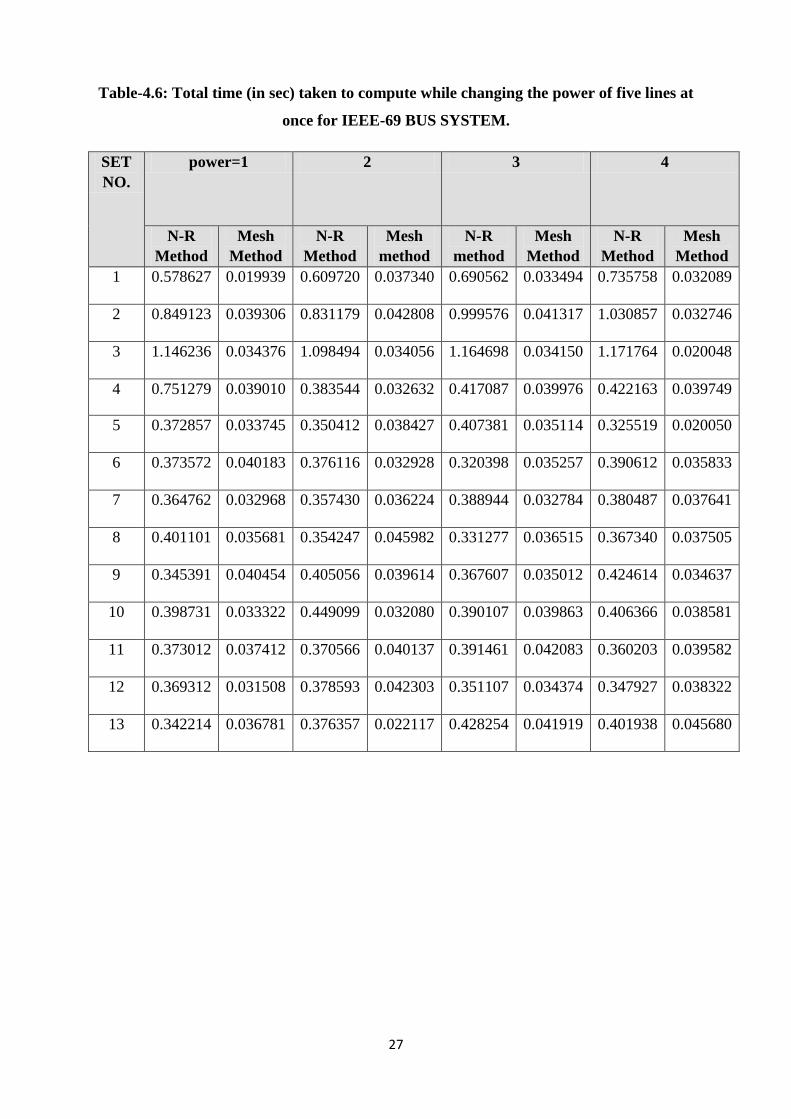
6. Table-4.6: Total time in seconds taken to compute while changing the power of five
lines at once for IEEE-69 BUS SYSTEM. 27
7. Table-6.1: Bus Data for IEEE-33 BUS SYSTEM. 36
8. Table-6.2: Line Data for IEEE-33 BUS SYSTEM. 37
9. Table-6.2: Mesh Data for IEEE-33 BUS SYSTEM. 37
10. Table-6.4: Bus Data for IEEE-69 BUS SYSTEM. 38
11. Table-6.5: Line Data for IEEE-69 BUS SYSTEM. 39
12. Table-6.3: Mesh Data for IEEE-69 BUS SYSTEM. 41

1
CHAPTER1
Introduction
2
1.1. LITERATURE AND REVIEW:
Delivery of electricity to end users is the final stage in the electricity distribution. A
distribution system network carries electricity from the transmission system and delivers it to
the consumers. Distribution networks are typically of two types:-
i). Radial distribution network
ii). Mesh distribution network.
A radial network leaves the station and passes through the network area with no
normal connection to any other supply. This is typical in long rural lines with isolated load
areas. An interconnected or meshed network is generally found in urban areas and will have
multiple connections to other points of supply.
The distribution system is entirely different, in both its operation and characteristics,
from the transmission system. The Newton-Raphson and Fast decoupled Methods have effi-
ciently solved the well behaved power system for the last two decades but they failed in case
of:-
i). Ill-conditioned or poorly initialized
ii). Special applications or special network structure, e.g. Meshed networks.[1,2,3]
The Gauss-Seidel power flow technique has also shown to be extremely inefficient
in solving large power systems [4].
Distribution networks, due to their wide ranging resistance and reactance values
and radial structure, fall into the category of ill-conditioned power systems for the generic
Newton-Raphson [5, 6] and fast decoupled power flow algorithms [7]. Even though with
some advancements in the Newton-Raphson Methods the robustness of the program is ob-
tained but still the computational time is large enough [8]. Thus to solve the distribution load
flow problems an algorithm is required which is having the following characteristics:
i). Capable of solving radial and meshed distribution network with several thousand line
sections (branches) and nodes (buses).
ii). Robust and efficient.
3
iii). Requires less computational time.
The efficiency of such a power system is of at most importance as each optimization
study requires numerous power flow runs. Efficient power flow algorithm for solving single
and three phase radial distribution network has been extensively used by electric distribution
engineers. However these algorithms are not designed to solve meshed network [9, 10].
In this thesis, we worked on the method proposed by D. Shirmoharmnadi, H. W.
Hong, A. Semlyen and G. X. Luo for the solution of weakly meshed network [11]. In this
method if the network is meshed, the interconnected grid is first broken at a number of points
(breakpoints) in order to convert it into one radial network [11]. The radial network is solved
efficiently by the direct application of Kirchhoff's voltage and current laws (KVL and
KCL).The power flows at the breakpoints is then accounted for by injecting currents at their
two end nodes. The breakpoint currents are calculated using the multi-port compensation
methods [11]. In the presence of constant P Q loads, the network becomes nonlinear and
causes the compensation process to become iterative [11]. The solution of the radial network
with the additional current injections completes the solution of the meshed network.
The numerical efficiency of the proposed compensation-based power flow method
diminishes as the number of breakpoints required to convert the meshed network to the radial
configuration increases [11].
4
CHAPTER2
LOAD FLOW TECHNIQUES
FOR DISTRIBUTION
NETWORKS
5
2.1. RADIAL DISTRIBUTION NETWORK TECHNIQUE:
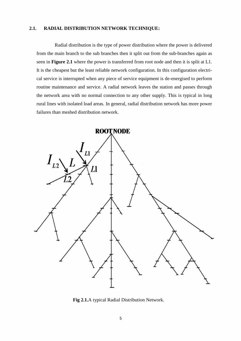
Radial distribution is the type of power distribution where the power is delivered
from the main branch to the sub branches then it split out from the sub-branches again as
seen in Figure 2.1 where the power is transferred from root node and then it is split at L1.
It is the cheapest but the least reliable network configuration. In this configuration electri-
cal service is interrupted when any piece of service equipment is de-energised to perform
routine maintenance and service. A radial network leaves the station and passes through
the network area with no normal connection to any other supply. This is typical in long
rural lines with isolated load areas. In general, radial distribution network has more power
failures than meshed distribution network.
Fig 2.1.A typical Radial Distribution Network.
6
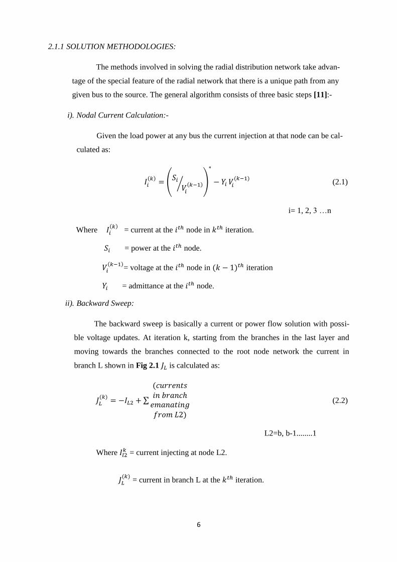
2.1.1 SOLUTION METHODOLOGIES:
The methods involved in solving the radial distribution network take advan-
tage of the special feature of the radial network that there is a unique path from any
given bus to the source. The general algorithm consists of three basic steps [11]:-
i). Nodal Current Calculation:-
Given the load power at any bus the current injection at that node can be cal-
culated as:
(2.1)
i= 1, 2, 3 …n
Where
= current at the node in iteration.
= power at the node.
= voltage at the node in iteration
= admittance at the node.
ii). Backward Sweep:
The backward sweep is basically a current or power flow solution with possi-
ble voltage updates. At iteration k, starting from the branches in the last layer and
moving towards the branches connected to the root node network the current in
branch L shown in Fig 2.1 is calculated as:
(2.2)
L2=b, b-1........1
Where = current injecting at node L2.
= current in branch L at the iteration.
7
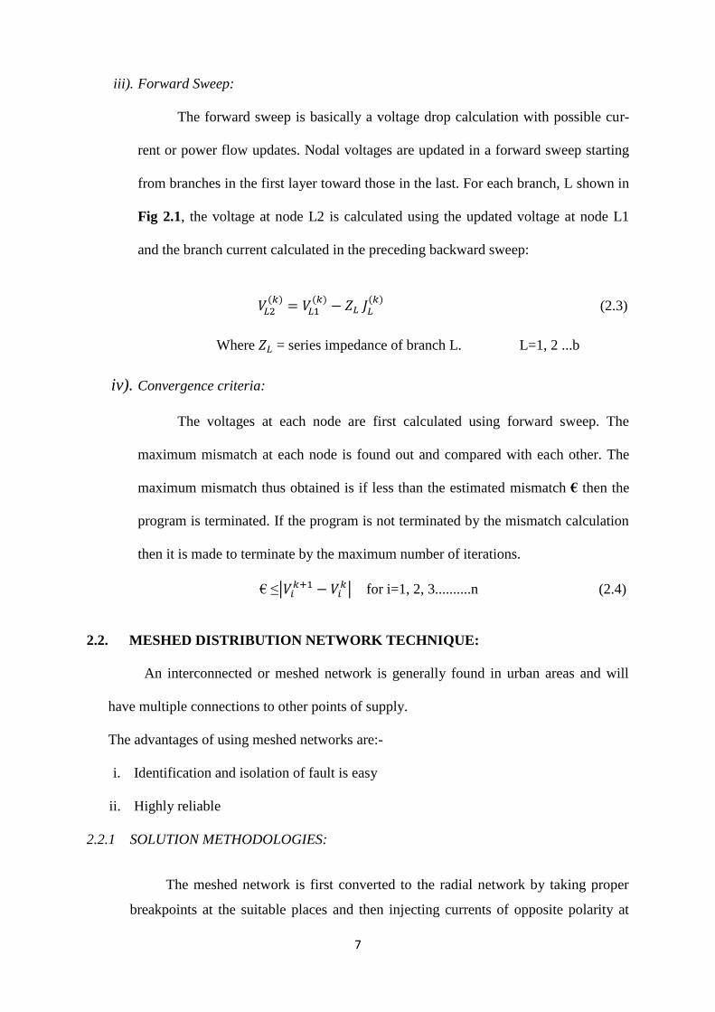
iii). Forward Sweep:
The forward sweep is basically a voltage drop calculation with possible cur-
rent or power flow updates. Nodal voltages are updated in a forward sweep starting
from branches in the first layer toward those in the last. For each branch, L shown in
Fig 2.1, the voltage at node L2 is calculated using the updated voltage at node L1
and the branch current calculated in the preceding backward sweep:
(2.3)
Where = series impedance of branch L. L=1, 2 ...b
iv). Convergence criteria:
The voltages at each node are first calculated using forward sweep. The
maximum mismatch at each node is found out and compared with each other. The
maximum mismatch thus obtained is if less than the estimated mismatch € then the
program is terminated. If the program is not terminated by the mismatch calculation
then it is made to terminate by the maximum number of iterations.
€ ≤
for i=1, 2, 3..........n (2.4)
2.2. MESHED DISTRIBUTION NETWORK TECHNIQUE:
An interconnected or meshed network is generally found in urban areas and will
have multiple connections to other points of supply.
The advantages of using meshed networks are:-
i. Identification and isolation of fault is easy
ii. Highly reliable
2.2.1 SOLUTION METHODOLOGIES:
The meshed network is first converted to the radial network by taking proper
breakpoints at the suitable places and then injecting currents of opposite polarity at
8
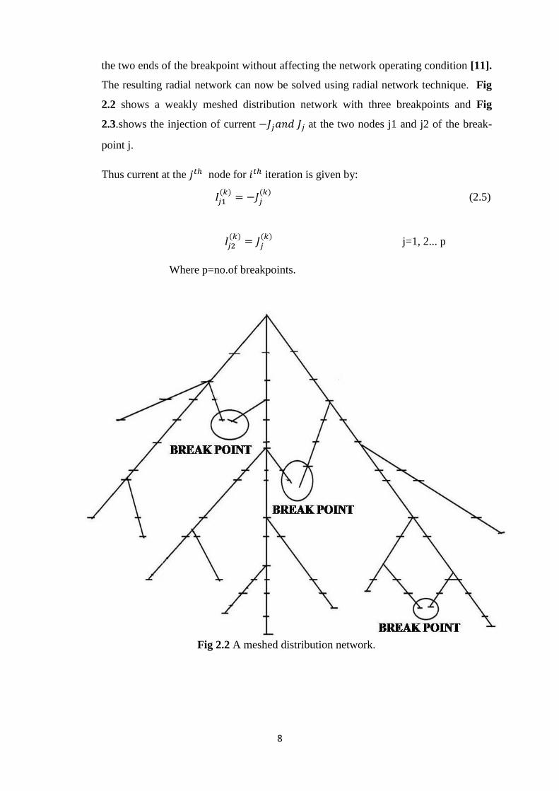
the two ends of the breakpoint without affecting the network operating condition [11].
The resulting radial network can now be solved using radial network technique. Fig
2.2 shows a weakly meshed distribution network with three breakpoints and Fig
2.3.shows the injection of current at the two nodes j1 and j2 of the break-
point j.
Thus current at the node for iteration is given by:
(2.5)
j=1, 2... p
Where p=no.of breakpoints.
Fig 2.2 A meshed distribution network.
9
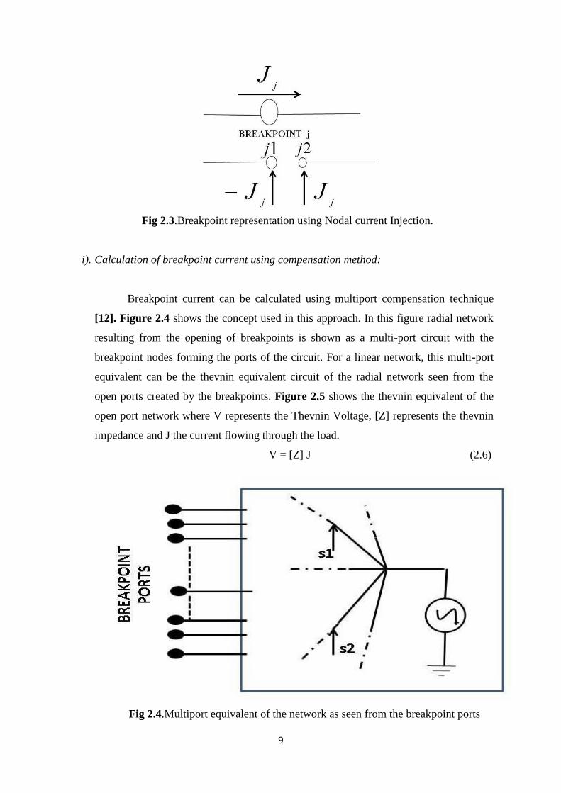
Fig 2.3.Breakpoint representation using Nodal current Injection.
i). Calculation of breakpoint current using compensation method:
Breakpoint current can be calculated using multiport compensation technique
[12]. Figure 2.4 shows the concept used in this approach. In this figure radial network
resulting from the opening of breakpoints is shown as a multi-port circuit with the
breakpoint nodes forming the ports of the circuit. For a linear network, this multi-port
equivalent can be the thevnin equivalent circuit of the radial network seen from the
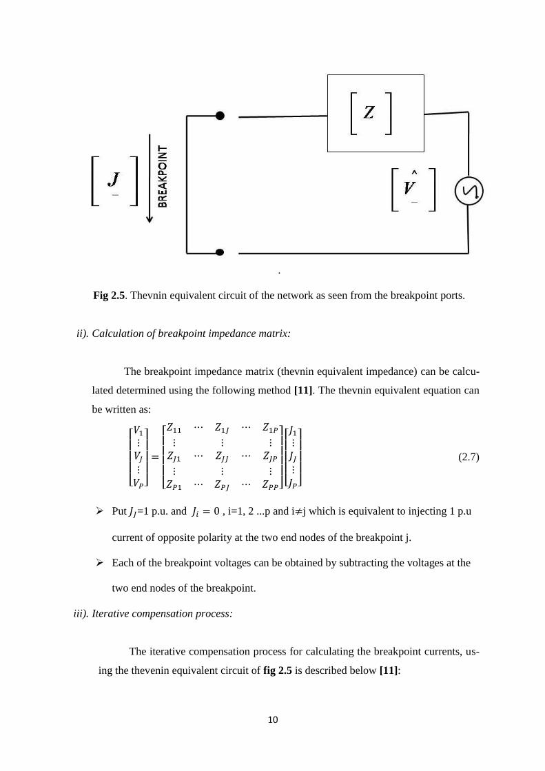
open ports created by the breakpoints. Figure 2.5 shows the thevnin equivalent of the
open port network where V represents the Thevnin Voltage, [Z] represents the thevnin
impedance and J the current flowing through the load.
V = [Z] J (2.6)
Fig 2.4.Multiport equivalent of the network as seen from the breakpoint ports
10
.
Fig 2.5. Thevnin equivalent circuit of the network as seen from the breakpoint ports.
ii). Calculation of breakpoint impedance matrix:
The breakpoint impedance matrix (thevnin equivalent impedance) can be calcu-
lated determined using the following method [11]. The thevnin equivalent equation can
be written as:
(2.7)
Put =1 p.u. and , i=1, 2 ...p and i j which is equivalent to injecting 1 p.u
current of opposite polarity at the two end nodes of the breakpoint j.
Each of the breakpoint voltages can be obtained by subtracting the voltages at the
two end nodes of the breakpoint.
iii). Iterative compensation process:
The iterative compensation process for calculating the breakpoint currents, us-
ing the thevenin equivalent circuit of fig 2.5 is described below [11]:
11
STEP 1. Calculate the thevenin equivalent impedance and maintain it constant
throughout the compensation process.
STEP 2. Calculate the thevenin equivalent voltage of the radial network including the
breakpoint currents calculated from the previous iteration of the compensa-
tion process assuming initial values of the breakpoint currents to be 0.
STEP 3. Calculate the incremental change in the breakpoint currents using the Theve-
nin equivalent circuit. At iteration m of the compensation process
(2.8)
STEP 4. Update the breakpoint currents. At iteration m:
(2.9)
STEP 5. Repeat equations 2, 3 and 4 until convergence is reached (the maximum
breakpoint voltage calculated at step 3 is within prescribed limits).
iv). Steps to solve meshed network:
The different steps involved in solving meshed distribution network are [11]:
STEP 1. First the bus and line data are read.
STEP 2. The meshed network is then converted to the radial network.
STEP 3. Branch numbering is done and the breakpoints are opened.
STEP 4. Breakpoint impedance matrix is then calculated.
STEP 5. Set iteration count to m=1 and solve the radial network load flow using
Forward Backward Sweep.
STEP 6. If the maximum voltage mismatch is less than the specified voltage
mismatch the exit the loop and print the result.
STEP 7. Else calculate the breakpoint currents and add them to nodal current.
STEP 8. If the maximum iteration is reached and still specified voltage
mismatch is not obtained then stop the process and print the result.
12
STEP 9. Else increase the iteration number by 1 and go to step 6 and repeat the
process till convergence point or the maximum iteration is reached.
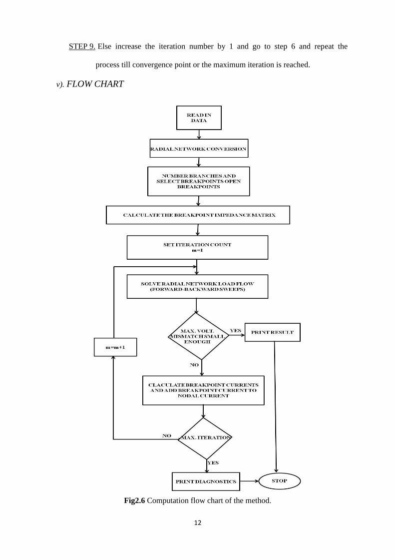
v). FLOW CHART
Fig2.6 Computation flow chart of the method.
13
CHAPTER3
MESH DISTRIBUTION
SYSTEM LOAD FLOW
TECHNIQUE VS NEWTON-
RAPHSON TECHNIQUE
14
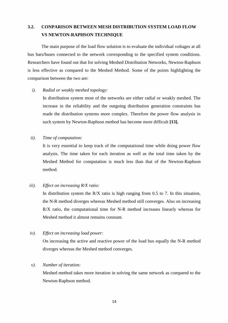
3.2. CONPARISON BETWEEN MESH DISTRIBUTION SYSTEM LOAD FLOW
VS NEWTON-RAPHSON TECHNIQUE The main purpose of the load flow solution is to evaluate the individual voltages at all
bus bars/buses connected to the network corresponding to the specified system conditions.
Researchers have found out that for solving Meshed Distribution Networks, Newton-Raphson
is less effective as compared to the Meshed Method. Some of the points highlighting the
comparison between the two are:
i). Radial or weakly meshed topology:
In distribution system most of the networks are either radial or weakly meshed. The
increase in the reliability and the outgoing distribution generation constraints has
made the distribution systems more complex. Therefore the power flow analysis in
such system by Newton-Raphson method has become more difficult [13].
ii). Time of computation:
It is very essential to keep track of the computational time while doing power flow
analysis. The time taken for each iteration as well as the total time taken by the
Meshed Method for computation is much less than that of the Newton-Raphson
method.
iii). Effect on increasing R/X ratio:
In distribution system the R/X ratio is high ranging from 0.5 to 7. In this situation,
the N-R method diverges whereas Meshed method still converges. Also on increasing
R/X ratio, the computational time for N-R method increases linearly whereas for
Meshed method it almost remains constant.
iv). Effect on increasing load power:
On increasing the active and reactive power of the load bus equally the N-R method
diverges whereas the Meshed method converges.
v). Number of iteration:
Meshed method takes more iteration in solving the same network as compared to the
Newton-Raphson method.

15
CHAPTER4
SIMULATION RESULTS
AND DISCUSSIONS
16
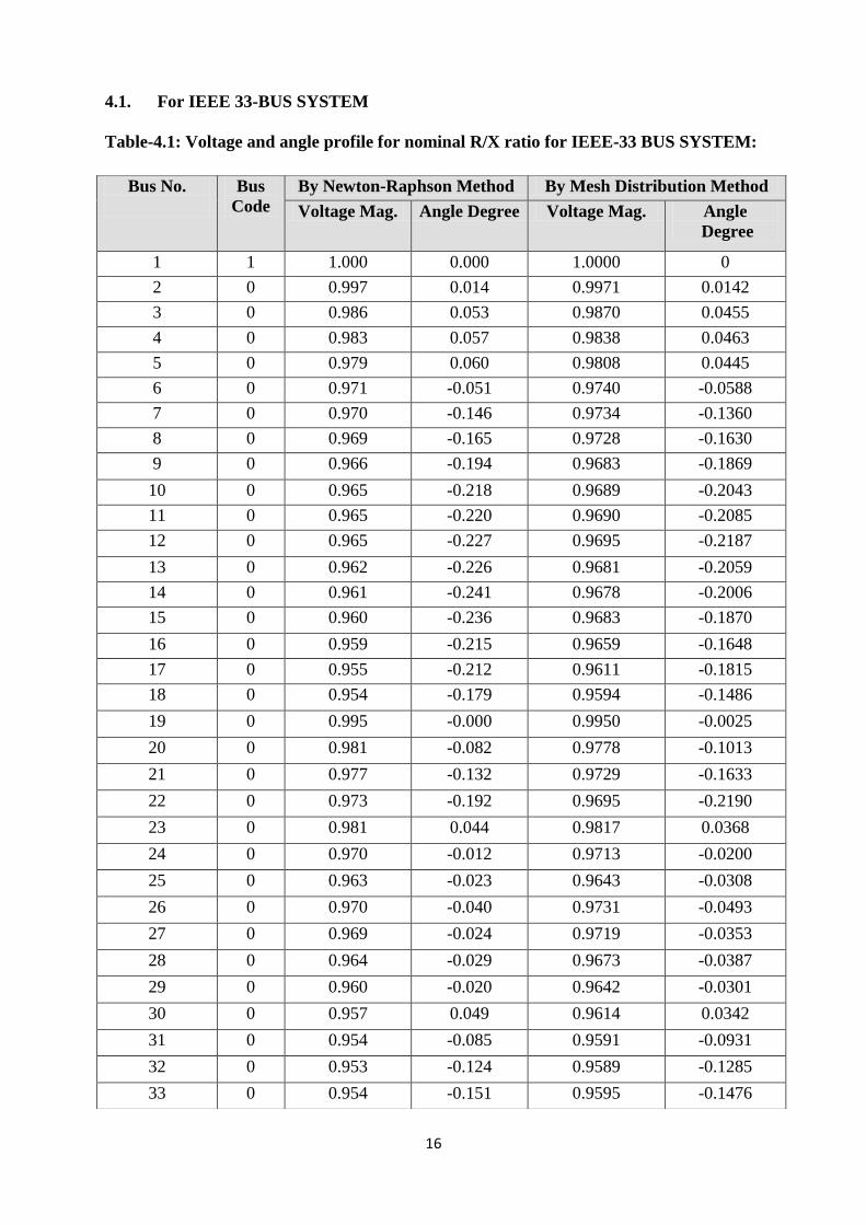
4.1. For IEEE 33-BUS SYSTEM
Table-4.1: Voltage and angle profile for nominal R/X ratio for IEEE-33 BUS SYSTEM:
Bus No.
Bus
Code
By Newton-Raphson Method By Mesh Distribution Method
Voltage Mag. Angle Degree Voltage Mag. Angle
Degree
1 1 1.000 0.000 1.0000 0
2 0 0.997 0.014 0.9971 0.0142
3 0 0.986 0.053 0.9870 0.0455
4 0 0.983 0.057 0.9838 0.0463
5 0 0.979 0.060 0.9808 0.0445
6 0 0.971 -0.051 0.9740 -0.0588
7 0 0.970 -0.146 0.9734 -0.1360
8 0 0.969 -0.165 0.9728 -0.1630
9 0 0.966 -0.194 0.9683 -0.1869
10 0 0.965 -0.218 0.9689 -0.2043
11 0 0.965 -0.220 0.9690 -0.2085
12 0 0.965 -0.227 0.9695 -0.2187
13 0 0.962 -0.226 0.9681 -0.2059
14 0 0.961 -0.241 0.9678 -0.2006
15 0 0.960 -0.236 0.9683 -0.1870
16 0 0.959 -0.215 0.9659 -0.1648
17 0 0.955 -0.212 0.9611 -0.1815
18 0 0.954 -0.179 0.9594 -0.1486
19 0 0.995 -0.000 0.9950 -0.0025
20 0 0.981 -0.082 0.9778 -0.1013
21 0 0.977 -0.132 0.9729 -0.1633
22 0 0.973 -0.192 0.9695 -0.2190
23 0 0.981 0.044 0.9817 0.0368
24 0 0.970 -0.012 0.9713 -0.0200
25 0 0.963 -0.023 0.9643 -0.0308
26 0 0.970 -0.040 0.9731 -0.0493
27 0 0.969 -0.024 0.9719 -0.0353
28 0 0.964 -0.029 0.9673 -0.0387
29 0 0.960 -0.020 0.9642 -0.0301
30 0 0.957 0.049 0.9614 0.0342
31 0 0.954 -0.085 0.9591 -0.0931
32 0 0.953 -0.124 0.9589 -0.1285
33 0 0.954 -0.151 0.9595 -0.1476
17
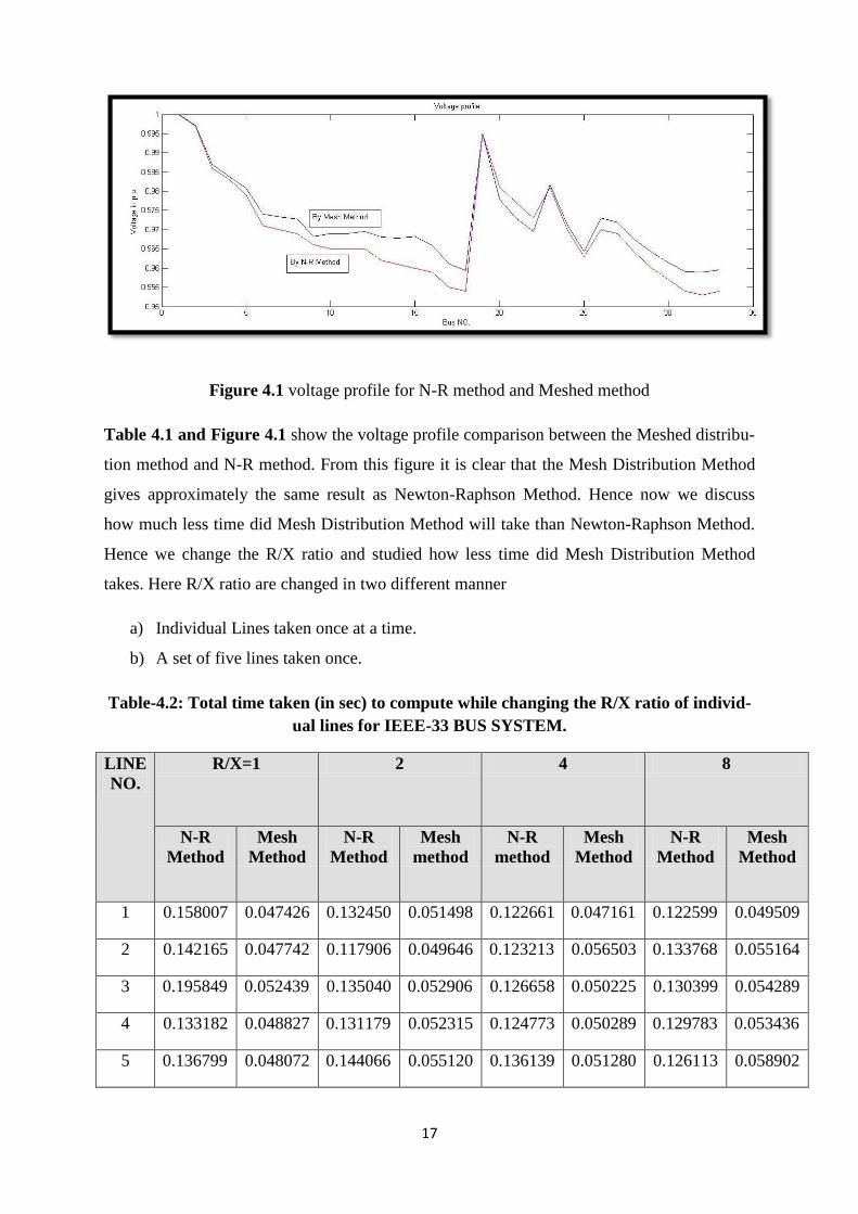
Figure 4.1 voltage profile for N-R method and Meshed method
Table 4.1 and Figure 4.1 show the voltage profile comparison between the Meshed distribu-
tion method and N-R method. From this figure it is clear that the Mesh Distribution Method
gives approximately the same result as Newton-Raphson Method. Hence now we discuss
how much less time did Mesh Distribution Method will take than Newton-Raphson Method.
Hence we change the R/X ratio and studied how less time did Mesh Distribution Method
takes. Here R/X ratio are changed in two different manner
a) Individual Lines taken once at a time.
b) A set of five lines taken once.
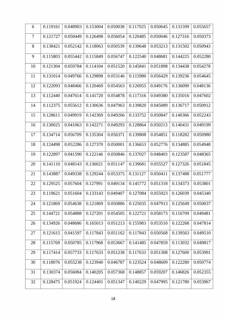
Table-4.2: Total time taken (in sec) to compute while changing the R/X ratio of individ-
ual lines for IEEE-33 BUS SYSTEM.
LINE
NO.
R/X=1 2 4 8
N-R
Method
Mesh
Method
N-R
Method
Mesh
method
N-R
method
Mesh
Method
N-R
Method
Mesh
Method
1 0.158007 0.047426 0.132450 0.051498 0.122661 0.047161 0.122599 0.049509
2 0.142165 0.047742 0.117906 0.049646 0.123213 0.056503 0.133768 0.055164
3 0.195849 0.052439 0.135040 0.052906 0.126658 0.050225 0.130399 0.054289
4 0.133182 0.048827 0.131179 0.052315 0.124773 0.050289 0.129783 0.053436
5 0.136799 0.048072 0.144066 0.055120 0.136139 0.051280 0.126113 0.058902
18
6 0.119161 0.048903 0.153004 0.050038 0.117025 0.050645 0.131599 0.055657
7 0.121727 0.050449 0.126498 0.056054 0.120485 0.050046 0.127316 0.050373
8 0.138421 0.052142 0.118063 0.050539 0.139648 0.053213 0.131502 0.050943
9 0.115803 0.055442 0.115849 0.056747 0.122540 0.048681 0.144225 0.052280
10 0.121304 0.059784 0.114104 0.051520 0.145841 0.051898 0.134438 0.054278
11 0.131014 0.049766 0.129898 0.053146 0.115980 0.056429 0.139236 0.054645
12 0.122093 0.048466 0.120469 0.054563 0.126955 0.049176 0.136090 0.048136
13 0.112440 0.047614 0.141720 0.054878 0.117316 0.049380 0.135016 0.047602
14 0.112375 0.055612 0.130636 0.047963 0.139820 0.045089 0.136717 0.050912
15 0.128611 0.049919 0.142369 0.049266 0.133752 0.050847 0.140366 0.052243
16 0.130025 0.041063 0.142271 0.049293 0.128864 0.050213 0.140431 0.049199
17 0.134714 0.056709 0.135304 0.056371 0.139808 0.054851 0.118282 0.050980
18 0.124498 0.052286 0.127370 0.050001 0.136653 0.052776 0.134885 0.054948
19 0.122897 0.041590 0.122146 0.050846 0.137027 0.048403 0.123587 0.048365
20 0.141110 0.048143 0.136021 0.051147 0.139681 0.055527 0.127326 0.051845
21 0.143887 0.049338 0.129244 0.053375 0.131127 0.050411 0.137488 0.051777
22 0.129525 0.057604 0.127991 0.049134 0.145772 0.051318 0.134373 0.053801
23 0.119621 0.051604 0.133143 0.049407 0.127084 0.055923 0.126039 0.045340
24 0.121869 0.054638 0.121869 0.050886 0.125035 0.047913 0.125649 0.050037
25 0.144721 0.054888 0.127201 0.054505 0.122721 0.058173 0.116709 0.049481
26 0.134926 0.048686 0.165013 0.051213 0.155983 0.053510 0.122268 0.047814
27 0.121615 0.041597 0.117843 0.051162 0.117843 0.050568 0.139563 0.049510
28 0.115769 0.050785 0.117968 0.053667 0.141485 0.047859 0.113032 0.049817
29 0.117414 0.057733 0.117633 0.051238 0.117633 0.051308 0.127600 0.053991
30 0.118076 0.055238 0.123940 0.046787 0.123524 0.048609 0.122280 0.050774
31 0.130374 0.056084 0.140205 0.057368 0.148857 0.059207 0.146826 0.052355
32 0.128475 0.051924 0.124401 0.051347 0.140229 0.047995 0.121780 0.053967
19
Table-4.3: Total time taken (in sec) to compute while changing the R/X ratio of five lines
at once for IEEE-33 BUS SYSTEM.
SET
NO.
R/X=1 2 4 8
N-R
Method
Mesh
Method
N-R
Method
Mesh
method
N-R
method
Mesh
Method
N-R
Method
Mesh
Method
1 0.128082 0.045388 0.122347 0.051872 0.128248 0.050721 0.138833 0.052760
2 0.111066 0.054062 0.139027 0.056423 0.140607 0.048765 0.141308 0.050312
3 0.119139 0.054931 0.119216 0.048071 0.121475 0.055238 0.157311 0.056368
4 0.114721 0.048573 0.136092 0.048528 0.117189 0.047311 0.125704 0.054812
5 0.137468 0.054510 0.134497 0.046777 0.139603 0.052825 0.133209 0.053936
6 0.117739 0.048729 0.122269 0.050348 0.114022 0.048168 0.152080 0.053243
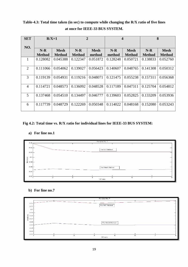
Fig 4.2: Total time vs. R/X ratio for individual lines for IEEE-33 BUS SYSTEM:
a) For line no.1
b) For line no.7
20
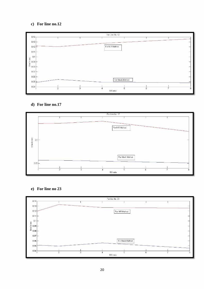
c) For line no.12
d) For line no.17
e) For line no 23
21
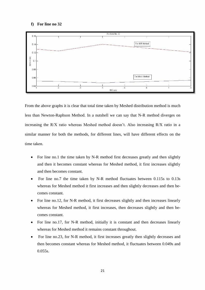
f) For line no 32
From the above graphs it is clear that total time taken by Meshed distribution method is much
less than Newton-Raphson Method. In a nutshell we can say that N-R method diverges on
increasing the R/X ratio whereas Meshed method doesn’t. Also increasing R/X ratio in a
similar manner for both the methods, for different lines, will have different effects on the
time taken.
For line no.1 the time taken by N-R method first decreases greatly and then slightly
and then it becomes constant whereas for Meshed method, it first increases slightly
and then becomes constant.
For line no.7 the time taken by N-R method fluctuates between 0.115s to 0.13s
whereas for Meshed method it first increases and then slightly decreases and then be-
comes constant.
For line no.12, for N-R method, it first decreases slightly and then increases linearly
whereas for Meshed method, it first increases, then decreases slightly and then be-
comes constant.
For line no.17, for N-R method, initially it is constant and then decreases linearly
whereas for Meshed method it remains constant throughout.
For line no.23, for N-R method, it first increases greatly then slightly decreases and
then becomes constant whereas for Meshed method, it fluctuates between 0.049s and
0.055s.
22
For line no.32, for N-R method, it fluctuates between 0.12s and 0.14s whereas for
Meshed method it almost remains constant.
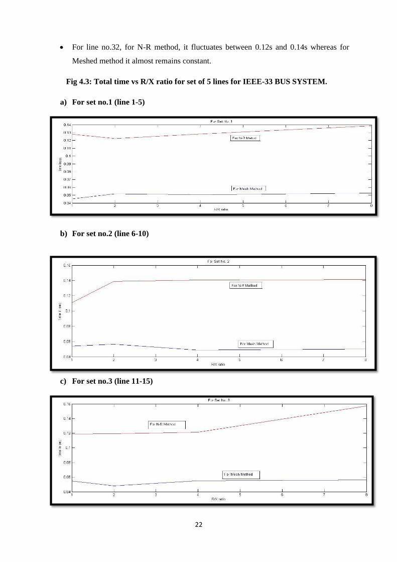
Fig 4.3: Total time vs R/X ratio for set of 5 lines for IEEE-33 BUS SYSTEM.
a) For set no.1 (line 1-5)
b) For set no.2 (line 6-10)
c) For set no.3 (line 11-15)
23
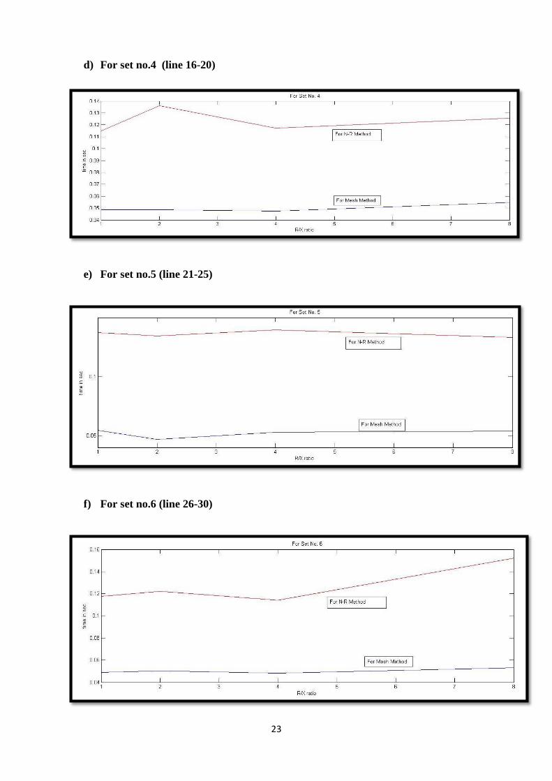
d) For set no.4 (line 16-20)
e) For set no.5 (line 21-25)
f) For set no.6 (line 26-30)
24
From the above graphs it is clear that when R/X ratio is increased from 1 to 8 in a set of five
lines simultaneously then the time of computation for N-R method increases greatly whereas
those for Meshed method remains constant. Thus the N-R method diverges on increasing the
R/X ratio whereas Meshed method doesn’t.
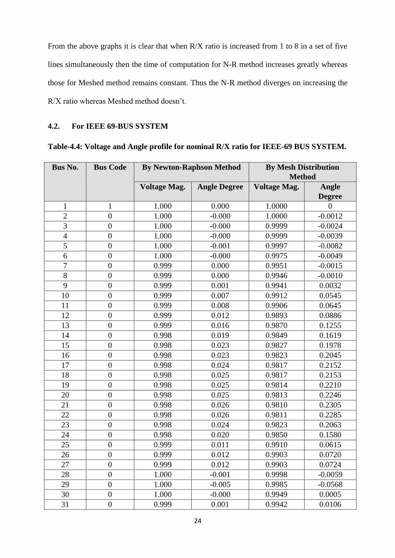
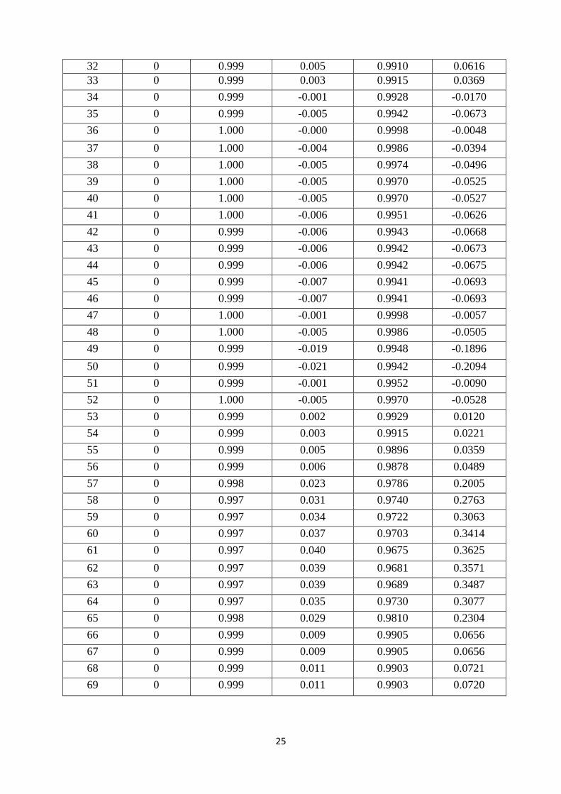
4.2. For IEEE 69-BUS SYSTEM
Table-4.4: Voltage and Angle profile for nominal R/X ratio for IEEE-69 BUS SYSTEM.
Bus No.
Bus Code By Newton-Raphson Method By Mesh Distribution
Method
Voltage Mag. Angle Degree Voltage Mag. Angle
Degree
1 1 1.000 0.000 1.0000 0
2 0 1.000 -0.000 1.0000 -0.0012
3 0 1.000 -0.000 0.9999 -0.0024
4 0 1.000 -0.000 0.9999 -0.0039
5 0 1.000 -0.001 0.9997 -0.0082
6 0 1.000 -0.000 0.9975 -0.0049
7 0 0.999 0.000 0.9951 -0.0015
8 0 0.999 0.000 0.9946 -0.0010
9 0 0.999 0.001 0.9941 0.0032
10 0 0.999 0.007 0.9912 0.0545
11 0 0.999 0.008 0.9906 0.0645
12 0 0.999 0.012 0.9893 0.0886
13 0 0.999 0.016 0.9870 0.1255
14 0 0.998 0.019 0.9849 0.1619
15 0 0.998 0.023 0.9827 0.1978
16 0 0.998 0.023 0.9823 0.2045
17 0 0.998 0.024 0.9817 0.2152
18 0 0.998 0.025 0.9817 0.2153
19 0 0.998 0.025 0.9814 0.2210
20 0 0.998 0.025 0.9813 0.2246
21 0 0.998 0.026 0.9810 0.2305
22 0 0.998 0.026 0.9811 0.2285
23 0 0.998 0.024 0.9823 0.2063
24 0 0.998 0.020 0.9850 0.1580
25 0 0.999 0.011 0.9910 0.0615
26 0 0.999 0.012 0.9903 0.0720
27 0 0.999 0.012 0.9903 0.0724
28 0 1.000 -0.001 0.9998 -0.0059
29 0 1.000 -0.005 0.9985 -0.0568
30 0 1.000 -0.000 0.9949 0.0005
31 0 0.999 0.001 0.9942 0.0106
25
32 0 0.999 0.005 0.9910 0.0616
33 0 0.999 0.003 0.9915 0.0369
34 0 0.999 -0.001 0.9928 -0.0170
35 0 0.999 -0.005 0.9942 -0.0673
36 0 1.000 -0.000 0.9998 -0.0048
37 0 1.000 -0.004 0.9986 -0.0394
38 0 1.000 -0.005 0.9974 -0.0496
39 0 1.000 -0.005 0.9970 -0.0525
40 0 1.000 -0.005 0.9970 -0.0527
41 0 1.000 -0.006 0.9951 -0.0626
42 0 0.999 -0.006 0.9943 -0.0668
43 0 0.999 -0.006 0.9942 -0.0673
44 0 0.999 -0.006 0.9942 -0.0675
45 0 0.999 -0.007 0.9941 -0.0693
46 0 0.999 -0.007 0.9941 -0.0693
47 0 1.000 -0.001 0.9998 -0.0057
48 0 1.000 -0.005 0.9986 -0.0505
49 0 0.999 -0.019 0.9948 -0.1896
50 0 0.999 -0.021 0.9942 -0.2094
51 0 0.999 -0.001 0.9952 -0.0090
52 0 1.000 -0.005 0.9970 -0.0528
53 0 0.999 0.002 0.9929 0.0120
54 0 0.999 0.003 0.9915 0.0221
55 0 0.999 0.005 0.9896 0.0359
56 0 0.999 0.006 0.9878 0.0489
57 0 0.998 0.023 0.9786 0.2005
58 0 0.997 0.031 0.9740 0.2763
59 0 0.997 0.034 0.9722 0.3063
60 0 0.997 0.037 0.9703 0.3414
61 0 0.997 0.040 0.9675 0.3625
62 0 0.997 0.039 0.9681 0.3571
63 0 0.997 0.039 0.9689 0.3487
64 0 0.997 0.035 0.9730 0.3077
65 0 0.998 0.029 0.9810 0.2304
66 0 0.999 0.009 0.9905 0.0656
67 0 0.999 0.009 0.9905 0.0656
68 0 0.999 0.011 0.9903 0.0721
69 0 0.999 0.011 0.9903 0.0720
26
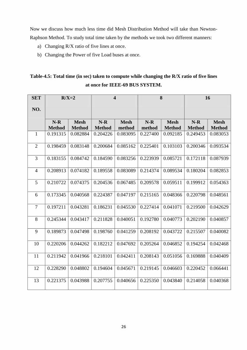
Now we discuss how much less time did Mesh Distribution Method will take than Newton-
Raphson Method. To study total time taken by the methods we took two different manners:
a) Changing R/X ratio of five lines at once.
b) Changing the Power of five Load buses at once.
Table-4.5: Total time (in sec) taken to compute while changing the R/X ratio of five lines
at once for IEEE-69 BUS SYSTEM.
SET
NO.
R/X=2 4 8 16
N-R
Method
Mesh
Method
N-R
Method
Mesh
method
N-R
method
Mesh
Method
N-R
Method
Mesh
Method
1 0.191315 0.082884 0.204226 0.083095 0.227400 0.092185 0.249453 0.083053
2 0.198459 0.083148 0.200684 0.085162 0.225401 0.103103 0.200346 0.093534
3 0.183155 0.084742 0.184590 0.083256 0.223939 0.085721 0.172118 0.087939
4 0.208913 0.074182 0.189558 0.083089 0.214374 0.089534 0.180204 0.082853
5 0.210722 0.074375 0.204536 0.067485 0.209578 0.059511 0.199912 0.054363
6 0.173345 0.040568 0.224387 0.047197 0.215165 0.048366 0.220798 0.048561
7 0.197211 0.043281 0.186231 0.045530 0.227414 0.041071 0.219500 0.042629
8 0.245344 0.043417 0.211828 0.040051 0.192780 0.040773 0.202190 0.040857
9 0.189873 0.047498 0.198760 0.041259 0.208192 0.043722 0.215507 0.040082
10 0.220206 0.044262 0.182212 0.047692 0.205264 0.046852 0.194254 0.042468
11 0.211942 0.041966 0.218101 0.042411 0.208143 0.051056 0.169888 0.040409
12 0.228290 0.048802 0.194604 0.045671 0.219145 0.046603 0.220452 0.066441
13 0.221375 0.043988 0.207755 0.040656 0.225350 0.043840 0.214058 0.040368
27
Table-4.6: Total time (in sec) taken to compute while changing the power of five lines at
once for IEEE-69 BUS SYSTEM.
SET
NO.
power=1 2 3 4
N-R
Method
Mesh
Method
N-R
Method
Mesh
method
N-R
method
Mesh
Method
N-R
Method
Mesh
Method
1 0.578627 0.019939 0.609720 0.037340 0.690562 0.033494 0.735758 0.032089
2 0.849123 0.039306 0.831179 0.042808 0.999576 0.041317 1.030857 0.032746
3 1.146236 0.034376 1.098494 0.034056 1.164698 0.034150 1.171764 0.020048
4 0.751279 0.039010 0.383544 0.032632 0.417087 0.039976 0.422163 0.039749
5 0.372857 0.033745 0.350412 0.038427 0.407381 0.035114 0.325519 0.020050
6 0.373572 0.040183 0.376116 0.032928 0.320398 0.035257 0.390612 0.035833
7 0.364762 0.032968 0.357430 0.036224 0.388944 0.032784 0.380487 0.037641
8 0.401101 0.035681 0.354247 0.045982 0.331277 0.036515 0.367340 0.037505
9 0.345391 0.040454 0.405056 0.039614 0.367607 0.035012 0.424614 0.034637
10 0.398731 0.033322 0.449099 0.032080 0.390107 0.039863 0.406366 0.038581
11 0.373012 0.037412 0.370566 0.040137 0.391461 0.042083 0.360203 0.039582
12 0.369312 0.031508 0.378593 0.042303 0.351107 0.034374 0.347927 0.038322
13 0.342214 0.036781 0.376357 0.022117 0.428254 0.041919 0.401938 0.045680
28
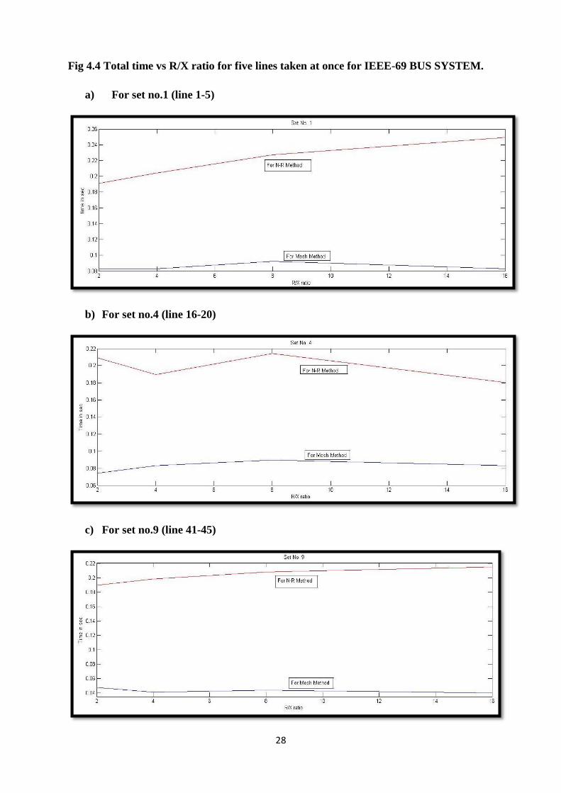
Fig 4.4 Total time vs R/X ratio for five lines taken at once for IEEE-69 BUS SYSTEM.
a) For set no.1 (line 1-5)
b) For set no.4 (line 16-20)
c) For set no.9 (line 41-45)
29
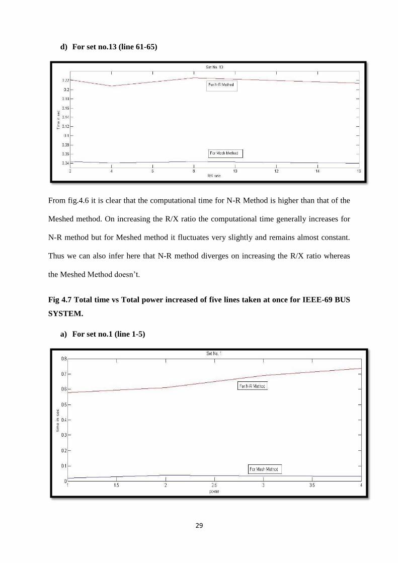
d) For set no.13 (line 61-65)
From fig.4.6 it is clear that the computational time for N-R Method is higher than that of the
Meshed method. On increasing the R/X ratio the computational time generally increases for
N-R method but for Meshed method it fluctuates very slightly and remains almost constant.
Thus we can also infer here that N-R method diverges on increasing the R/X ratio whereas
the Meshed Method doesn’t.
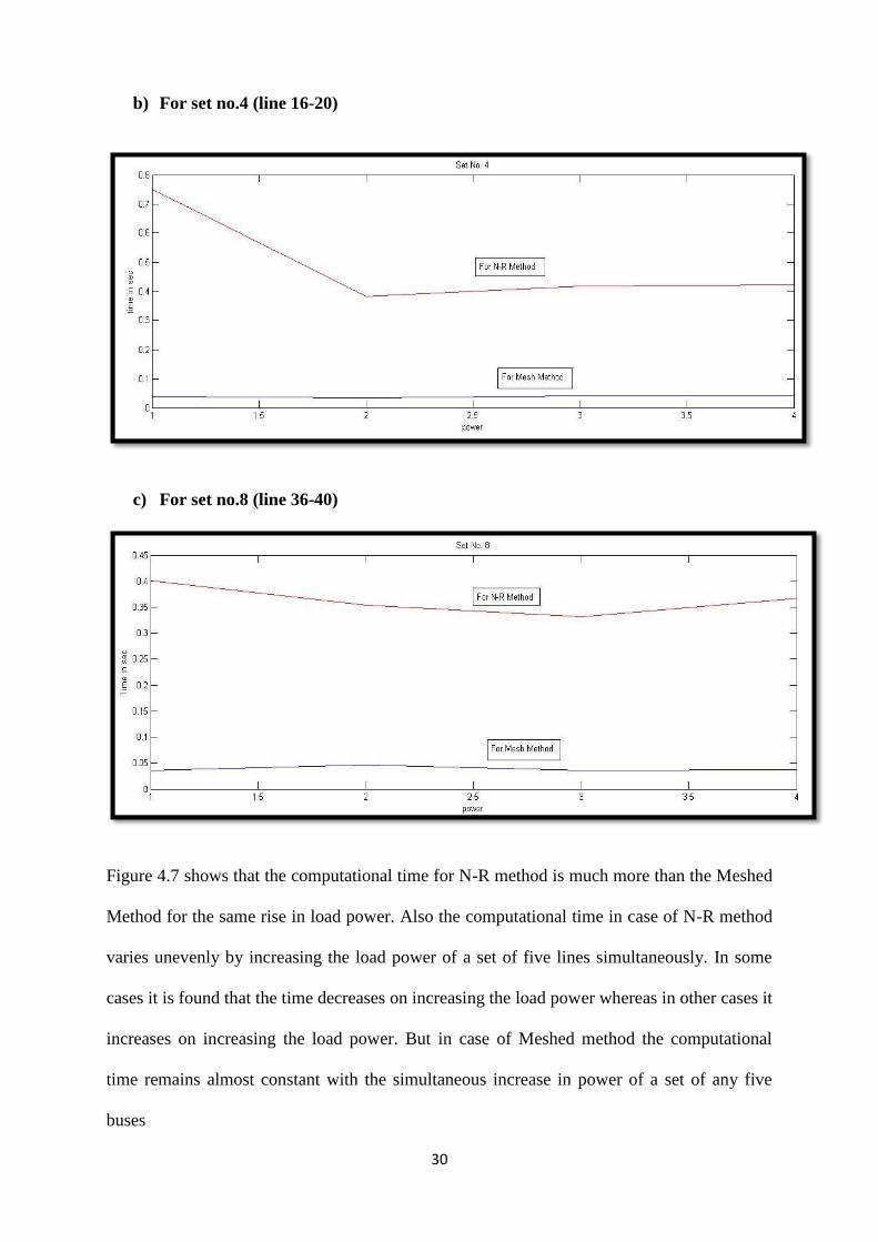
Fig 4.7 Total time vs Total power increased of five lines taken at once for IEEE-69 BUS
SYSTEM.
a) For set no.1 (line 1-5)
30
b) For set no.4 (line 16-20)
c) For set no.8 (line 36-40)
Figure 4.7 shows that the computational time for N-R method is much more than the Meshed
Method for the same rise in load power. Also the computational time in case of N-R method
varies unevenly by increasing the load power of a set of five lines simultaneously. In some
cases it is found that the time decreases on increasing the load power whereas in other cases it
increases on increasing the load power. But in case of Meshed method the computational
time remains almost constant with the simultaneous increase in power of a set of any five
buses

31
CHAPTER6
Conclusion

32
6.1 CONCLUSION:
The voltage and angle profile for the IEEE-33 BUS SYSTEM and IEEE-69 BUS SYSTEM
in the meshed distribution network is analysed using both Newton-Raphson method as well
as Meshed Distribution method. In both the cases the profile is almost same. The overall
computational time for N-R method is more than that of the Meshed method. Even though the
number of iteration taken by Meshed method is more than that of the N-R method but still the
time per iteration is lesser in case of Meshed method. It is also found out that on increasing
the R/X ratio the computational time for N-R method increases but for Meshed method it re-
mains almost constant. Also if R/X ratio is increased to a very high value then the N-R
method got diverged but the Meshed method is still converging. The computational time also
varies with the rise in load power. It is observed that in case of N-R method it varies un-
evenly i.e. sometime it raises but sometime it dips, whereas in case of meshed method the
computational time varies very slightly with the increase in load power.
33
REFERENCES
[1]. S.C.Tripathy, G.Durga Prasad, O.P.Malik and G.S.Hope, “Load Floaw for Ill-
Conditioned Power Systems By a Newton Like Method”, IEEE Trans., PAS-101, Oc-
tober 1982, pp.3648-3657.
[2]. S.Iwanato, Y.Tamura, “A Load Flow Calcultaion Method for Ill-Conditioned Power
Systems”, IEEE Trans., PAS-100,April 1981, pp. 1736-1743.
[3]. D.Rijicic, A.Bose, “A Modification to the Fast Decoupled Power Flow For Net-
workswith High R/X Ratios”, PICA 1987 Conference, Montreal, Canada.
[4]. C.L Wadhwa, “Electrical Power Systems”, New Age International, 2010 edition.
[5]. S.C. Tripathy, G.D. Prasad, O.P.Malik, and G.S.Hope,”Load Flow Solution for ill
conditioned power system by a Newton Raphson Like Method”,IEEE Trans, on
Power Apparatus and Systems; vol.PAS-101,No.10, October 1982, pp.3648-3657.
[6]. AradhanaPradhan and PadmajaThatoi, “Study On Performance Of Newton-Raphson
Load Flow In Distribution Syatems”, Department of Electrical Engineering, NIT
Rourkela, 2012.
[7]. K.Behnam-Guilani,”Fast Decoupled Load Flow: The Hybrid Model”,IEEE Trans. On
Power Systems, Vol.3, No.2, May 1988, pp.734-742.
[8]. G.X. LUO and A. Semlyen, “Efficient Load Flow For Large Weakly Meshed Net-
works”, IEEE Transactions on Power Systems, Vol. 5, No. 4, November 1990, pp-
1309 to 1313.
[9]. Jen-HaoTeng, “A Direct Approach for Distribution System Load Flow Solutions”,
IEEE TRANSACTIONS ON POWER DELIVERY, VOL. 18, NO. 3, JULY 2003,
pp-882.
[10]. Saadat H., “Power System Analysis”, Tata McGraw-Hill, New Delhi, 1999, 2002
edition

34
[11]. D.Shirmoharmnadi, H. W. Hong, A. Semlyen and G. X. Luo, “A Compensation-
Bsaed Power Flow Method For Weakly Meshed Distribution and Transmission
Networks”, IEEE Transactions on Power Systems, Vol. 3, No. 2, May 1988, pp-753
to 754.
[12]. W.F.Tinney, “Compensation Methods for Network Solutions by triangular factori
zation”, Proc.of PICA Conference, Boston, Mass., May 24-26, 1971.
[13]. W. H. Kersting, “A method to design and operation of a distribution system”, IEEE
Trans. Power Apparatus and Systems, PAS-103, pp. 1945–1952, 1984.

35
APPENDIX
36
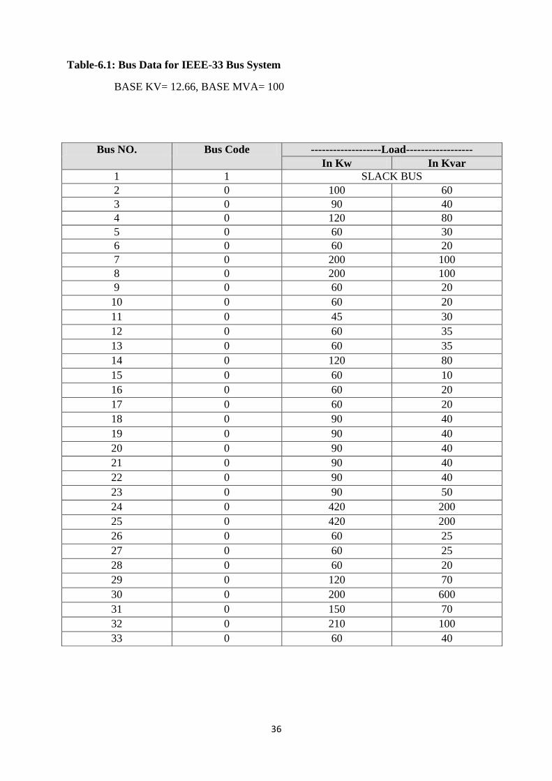
Table-6.1: Bus Data for IEEE-33 Bus System
BASE KV= 12.66, BASE MVA= 100
Bus NO. Bus Code -------------------Load------------------
In Kw In Kvar
1 1 SLACK BUS
2 0 100 60
3 0 90 40
4 0 120 80
5 0 60 30
6 0 60 20
7 0 200 100
8 0 200 100
9 0 60 20
10 0 60 20
11 0 45 30
12 0 60 35
13 0 60 35
14 0 120 80
15 0 60 10
16 0 60 20
17 0 60 20
18 0 90 40
19 0 90 40
20 0 90 40
21 0 90 40
22 0 90 40
23 0 90 50
24 0 420 200
25 0 420 200
26 0 60 25
27 0 60 25
28 0 60 20
29 0 120 70
30 0 200 600
31 0 150 70
32 0 210 100
33 0 60 40
37
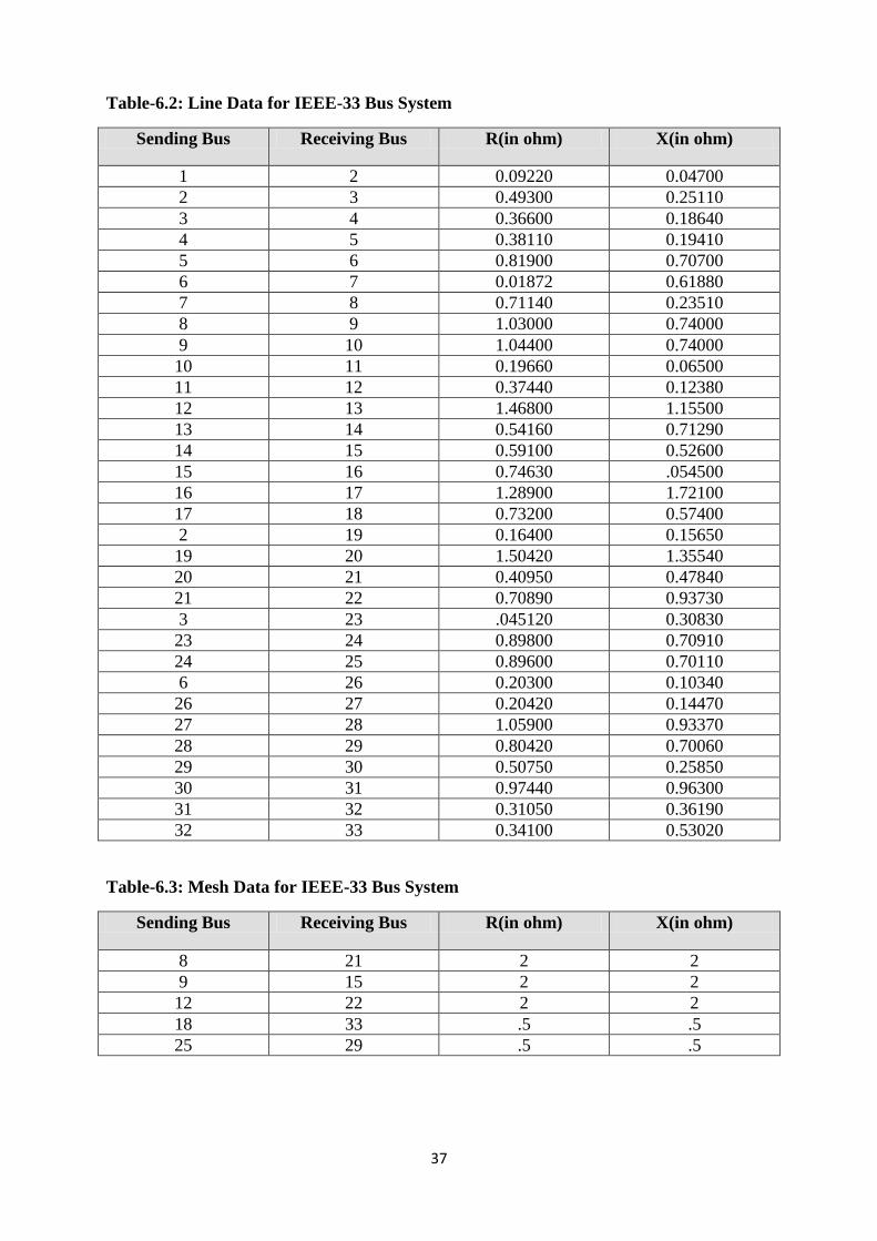
Table-6.2: Line Data for IEEE-33 Bus System
Sending Bus Receiving Bus R(in ohm) X(in ohm)
1 2 0.09220 0.04700
2 3 0.49300 0.25110
3 4 0.36600 0.18640
4 5 0.38110 0.19410
5 6 0.81900 0.70700
6 7 0.01872 0.61880
7 8 0.71140 0.23510
8 9 1.03000 0.74000
9 10 1.04400 0.74000
10 11 0.19660 0.06500
11 12 0.37440 0.12380
12 13 1.46800 1.15500
13 14 0.54160 0.71290
14 15 0.59100 0.52600
15 16 0.74630 .054500
16 17 1.28900 1.72100
17 18 0.73200 0.57400
2 19 0.16400 0.15650
19 20 1.50420 1.35540
20 21 0.40950 0.47840
21 22 0.70890 0.93730
3 23 .045120 0.30830
23 24 0.89800 0.70910
24 25 0.89600 0.70110
6 26 0.20300 0.10340
26 27 0.20420 0.14470
27 28 1.05900 0.93370
28 29 0.80420 0.70060
29 30 0.50750 0.25850
30 31 0.97440 0.96300
31 32 0.31050 0.36190
32 33 0.34100 0.53020
Table-6.3: Mesh Data for IEEE-33 Bus System
Sending Bus Receiving Bus R(in ohm) X(in ohm)
8 21 2 2
9 15 2 2
12 22 2 2
18 33 .5 .5
25 29 .5 .5
38
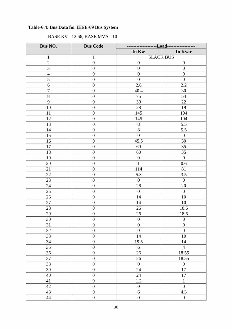
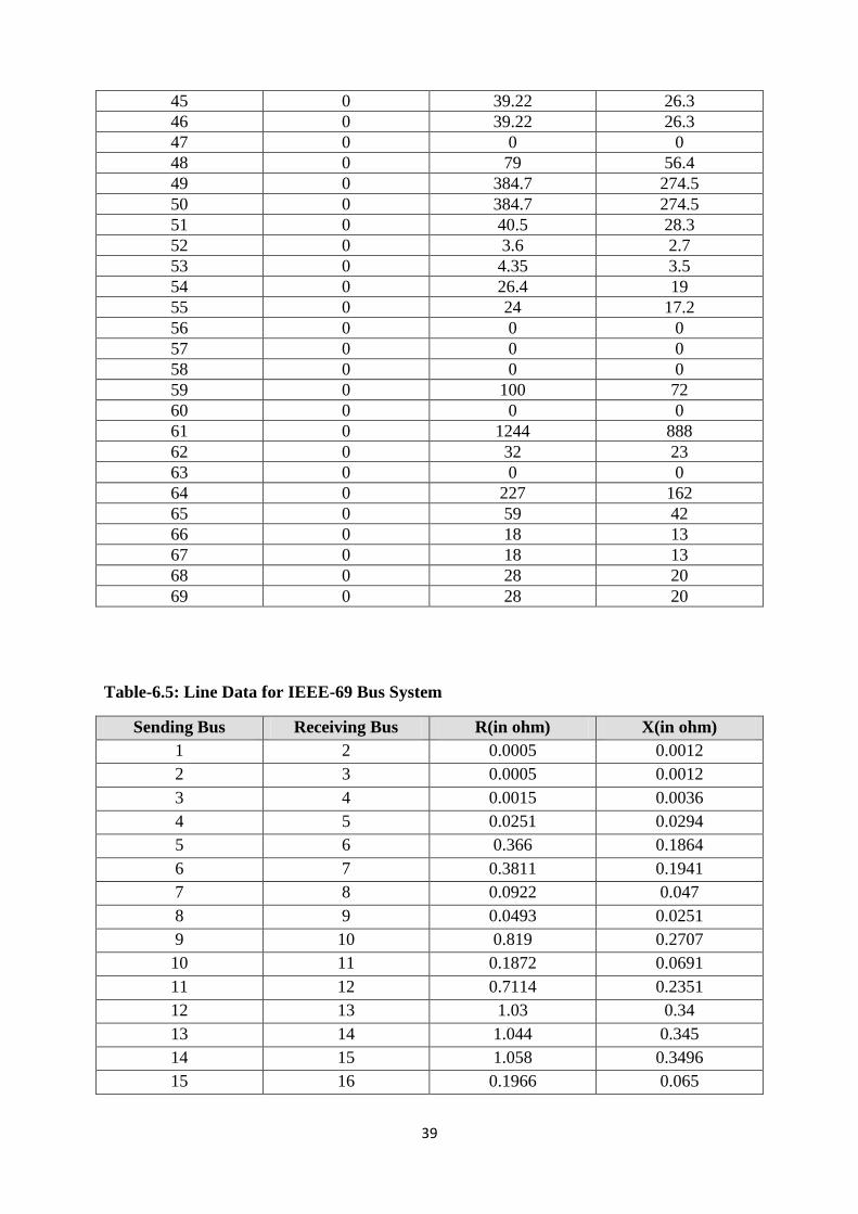
Table-6.4: Bus Data for IEEE-69 Bus System
BASE KV= 12.66, BASE MVA= 10
Bus NO. Bus Code -------------------Load------------------
In Kw In Kvar
1 1 SLACK BUS
2 0 0 0
3 0 0 0
4 0 0 0
5 0 0 0
6 0 2.6 2.2
7 0 40.4 30
8 0 75 54
9 0 30 22
10 0 28 19
11 0 145 104
12 0 145 104
13 0 8 5.5
14 0 8 5.5
15 0 0 0
16 0 45.5 30
17 0 60 35
18 0 60 35
19 0 0 0
20 0 1 0.6
21 0 114 81
22 0 5.3 3.5
23 0 0 0
24 0 28 20
25 0 0 0
26 0 14 10
27 0 14 10
28 0 26 18.6
29 0 26 18.6
30 0 0 0
31 0 0 0
32 0 0 0
33 0 14 10
34 0 19.5 14
35 0 6 4
36 0 26 18.55
37 0 26 18.55
38 0 0 0
39 0 24 17
40 0 24 17
41 0 1.2 1
42 0 0 0
43 0 6 4.3
44 0 0 0
39
45 0 39.22 26.3
46 0 39.22 26.3
47 0 0 0
48 0 79 56.4
49 0 384.7 274.5
50 0 384.7 274.5
51 0 40.5 28.3
52 0 3.6 2.7
53 0 4.35 3.5
54 0 26.4 19
55 0 24 17.2
56 0 0 0
57 0 0 0
58 0 0 0
59 0 100 72
60 0 0 0
61 0 1244 888
62 0 32 23
63 0 0 0
64 0 227 162
65 0 59 42
66 0 18 13
67 0 18 13
68 0 28 20
69 0 28 20
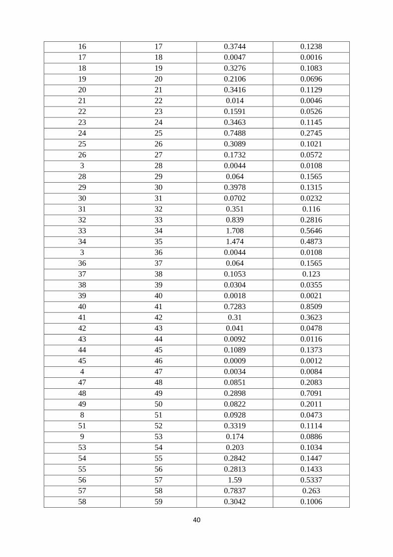
Table-6.5: Line Data for IEEE-69 Bus System
Sending Bus Receiving Bus R(in ohm) X(in ohm)
1 2 0.0005 0.0012
2 3 0.0005 0.0012
3 4 0.0015 0.0036
4 5 0.0251 0.0294
5 6 0.366 0.1864
6 7 0.3811 0.1941
7 8 0.0922 0.047
8 9 0.0493 0.0251
9 10 0.819 0.2707
10 11 0.1872 0.0691
11 12 0.7114 0.2351
12 13 1.03 0.34
13 14 1.044 0.345
14 15 1.058 0.3496
15 16 0.1966 0.065
40
16 17 0.3744 0.1238
17 18 0.0047 0.0016
18 19 0.3276 0.1083
19 20 0.2106 0.0696
20 21 0.3416 0.1129
21 22 0.014 0.0046
22 23 0.1591 0.0526
23 24 0.3463 0.1145
24 25 0.7488 0.2745
25 26 0.3089 0.1021
26 27 0.1732 0.0572
3 28 0.0044 0.0108
28 29 0.064 0.1565
29 30 0.3978 0.1315
30 31 0.0702 0.0232
31 32 0.351 0.116
32 33 0.839 0.2816
33 34 1.708 0.5646
34 35 1.474 0.4873
3 36 0.0044 0.0108
36 37 0.064 0.1565
37 38 0.1053 0.123
38 39 0.0304 0.0355
39 40 0.0018 0.0021
40 41 0.7283 0.8509
41 42 0.31 0.3623
42 43 0.041 0.0478
43 44 0.0092 0.0116
44 45 0.1089 0.1373
45 46 0.0009 0.0012
4 47 0.0034 0.0084
47 48 0.0851 0.2083
48 49 0.2898 0.7091
49 50 0.0822 0.2011
8 51 0.0928 0.0473
51 52 0.3319 0.1114
9 53 0.174 0.0886
53 54 0.203 0.1034
54 55 0.2842 0.1447
55 56 0.2813 0.1433
56 57 1.59 0.5337
57 58 0.7837 0.263
58 59 0.3042 0.1006
41
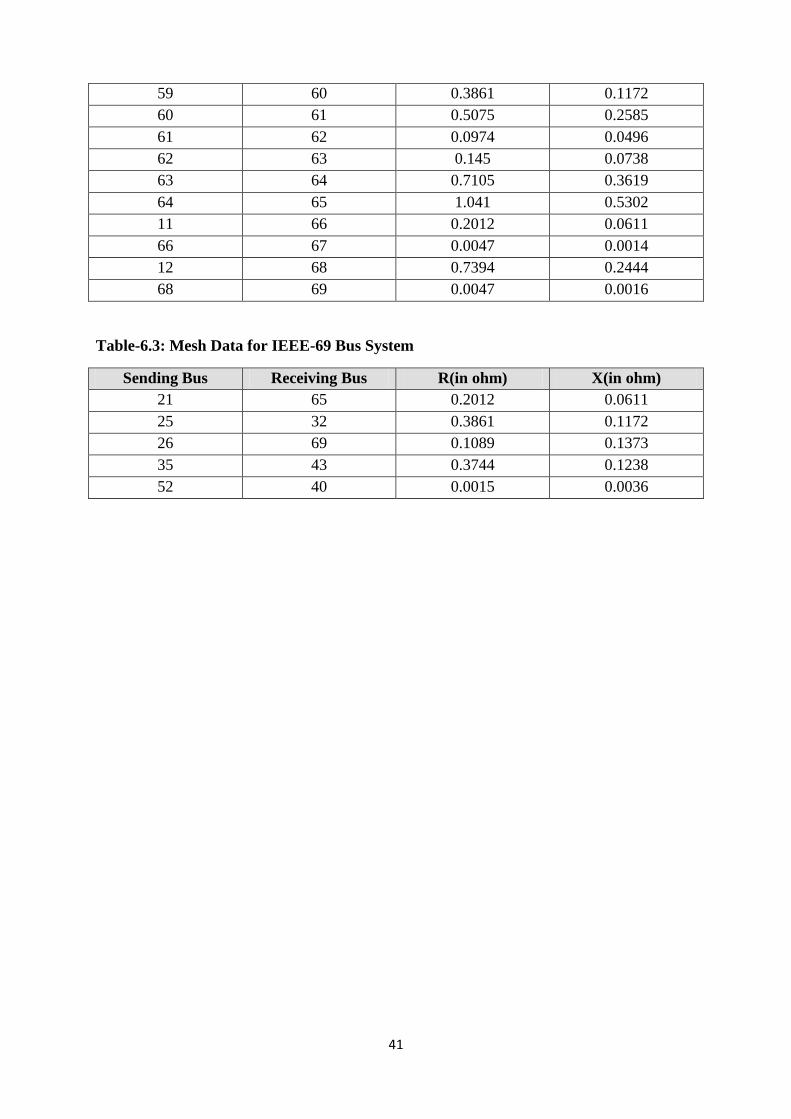
59 60 0.3861 0.1172
60 61 0.5075 0.2585
61 62 0.0974 0.0496
62 63 0.145 0.0738
63 64 0.7105 0.3619
64 65 1.041 0.5302
11 66 0.2012 0.0611
66 67 0.0047 0.0014
12 68 0.7394 0.2444
68 69 0.0047 0.0016
Table-6.3: Mesh Data for IEEE-69 Bus System
Sending Bus Receiving Bus R(in ohm) X(in ohm)
21 65 0.2012 0.0611
25 32 0.3861 0.1172
26 69 0.1089 0.1373
35 43 0.3744 0.1238
52 40 0.0015 0.0036


