MESHED PATCH ANTENNAS INTEGRATED ON SOLAR CELL - A

FEASIBILITY STUDY AND OPTIMIZATION

by

Timothy W. Turpin

A thesis submitted in partial fulfillmentof the requirements for the degree

of

MASTER OF SCIENCE

in

Electrical Engineering

Approved:

Dr. Reyhan Baktur Dr. Jacob GuntherMajor Professor Committee Member

Dr. Edmund Spencer Dr. Byron R. BurnhamCommittee Member Dean of Graduate Studies

UTAH STATE UNIVERSITYLogan, Utah

2008

ii

Copyright c© Timothy W. Turpin 2008

All Rights Reserved

iii

Abstract

Meshed Patch Antennas Integrated on Solar Cell - A Feasibility Study and Optimization

by

Timothy W. Turpin, Master of Science

Utah State University, 2008

Major Professor: Dr. Reyhan BakturDepartment: Electrical and Computer Engineering

This thesis work presents the feasibility of integrating meshed patch antennas directly

onto the solar cell assembly to save valuable surface real estate of a small satellite. The

solar cell cover glass is used as the substrate for the patch antenna. The antenna topology is

chosen to be a meshed patch so that it is transparent to light to ensure the proper operation

of solar cells. We found that although there is a compromise between the antenna efficiency

and see-through percentage, one is able to optimize the antenna by carefully designing the

mesh. To verify the design and integration, a meshed antenna operating at around 2.3

GHz is printed with conductive ink on a plastic substrate and placed on-top of solar cells

attached to an aluminum ground plane. The printed solar cell antenna is measured with

Nearfield Systems Inc. spherical near-field range and the measurements agree well with the

design.

(92 pages)

iv

Acknowledgments

I would like to thank my major professor, Dr. Reyhan Baktur, for giving me the

opportunity to work on this thesis project in the area of electromagnetic that I very much

enjoy. This opportunity also gave me the ability to continue my education here at Utah

State University for which I am very thankful. It has been a great learning experience that

I am grateful to have had. I would also like to thank her very much for the time and effort

she has put forth in the feedback and editing of the work; without her this thesis would not

have been possible. She was also instrumental in getting the near-field range functioning,

which was vital for this thesis.

I would also like to thank the other members of my committee, Dr. Jacob Gunther

and Dr. Edmund Spencer. Two professors who really demonstrate what it means to be an

educator, the desire and enthusiasm to help others better themselves through learning, and

always willing to help. I would also like to thank them for the time they have given to help

this thesis become a better product.

I would like to thank two of my professors from my undergraduate work: Dr. Michael

Tompkins, for instilling within me the love for electromagnetics; and Dr. Larry Smith of

Snow College, for showing me that if you want to learn, you need to work hard and it is

worth the effort, and to never give up and work to the end. Also special thanks to those

at Badger Screen printing for being willing to experiment and print the meshed antennas.

Finally, thanks to my family and friends who have supported me throughout my education.

Timothy W. Turpin

v

Contents

Page

Abstract . . . . . . . . . . . . . . . . . . . . . . . . . . . . . . . . . . . . . . . . . . . . . . . . . . . . . . . iii

Acknowledgments . . . . . . . . . . . . . . . . . . . . . . . . . . . . . . . . . . . . . . . . . . . . . . . iv

List of Tables . . . . . . . . . . . . . . . . . . . . . . . . . . . . . . . . . . . . . . . . . . . . . . . . . . . vii

List of Figures . . . . . . . . . . . . . . . . . . . . . . . . . . . . . . . . . . . . . . . . . . . . . . . . . . viii

1 Transparent Meshed Patch Antennas . . . . . . . . . . . . . . . . . . . . . . . . . . . . . 11.1 Introduction . . . . . . . . . . . . . . . . . . . . . . . . . . . . . . . . . . . . 11.2 Meshed Patch Antennas over Solid Ground Plane . . . . . . . . . . . . . . . 3

1.2.1 Meshed Patch Antenna Layouts . . . . . . . . . . . . . . . . . . . . . 41.2.2 Feeding . . . . . . . . . . . . . . . . . . . . . . . . . . . . . . . . . . 51.2.3 Impedance Calculations . . . . . . . . . . . . . . . . . . . . . . . . . 51.2.4 Momentum Simulations . . . . . . . . . . . . . . . . . . . . . . . . . 6

1.3 Fabrication with Wire Mesh . . . . . . . . . . . . . . . . . . . . . . . . . . . 71.3.1 Stub Tuning . . . . . . . . . . . . . . . . . . . . . . . . . . . . . . . 91.3.2 Probe Feed . . . . . . . . . . . . . . . . . . . . . . . . . . . . . . . . 10

2 Optimization of Meshed Patch Antennas . . . . . . . . . . . . . . . . . . . . . . . . . . 132.1 Optimization Via Line Width . . . . . . . . . . . . . . . . . . . . . . . . . . 13

2.1.1 HFSS Simulation . . . . . . . . . . . . . . . . . . . . . . . . . . . . . 132.1.2 Fabrication . . . . . . . . . . . . . . . . . . . . . . . . . . . . . . . . 182.1.3 Measurements . . . . . . . . . . . . . . . . . . . . . . . . . . . . . . 202.1.4 Conclusions . . . . . . . . . . . . . . . . . . . . . . . . . . . . . . . . 25

2.2 Optimization Via Orthogonal Lines . . . . . . . . . . . . . . . . . . . . . . . 262.2.1 HFSS Simulation . . . . . . . . . . . . . . . . . . . . . . . . . . . . . 262.2.2 Fabrication and Measurements . . . . . . . . . . . . . . . . . . . . . 292.2.3 Conclusions . . . . . . . . . . . . . . . . . . . . . . . . . . . . . . . . 30

3 Integration of Meshed Patch Antennas with Solar Cells . . . . . . . . . . . . . 333.1 Feeding . . . . . . . . . . . . . . . . . . . . . . . . . . . . . . . . . . . . . . 333.2 Effect of Conductivity . . . . . . . . . . . . . . . . . . . . . . . . . . . . . . 343.3 Fabrication . . . . . . . . . . . . . . . . . . . . . . . . . . . . . . . . . . . . 373.4 Measurments . . . . . . . . . . . . . . . . . . . . . . . . . . . . . . . . . . . 37

4 Conclusions . . . . . . . . . . . . . . . . . . . . . . . . . . . . . . . . . . . . . . . . . . . . . . . . . . 39

References . . . . . . . . . . . . . . . . . . . . . . . . . . . . . . . . . . . . . . . . . . . . . . . . . . . . . . 41

vi

Appendices . . . . . . . . . . . . . . . . . . . . . . . . . . . . . . . . . . . . . . . . . . . . . . . . . . . . . 43Appendix A HFSS Scripting . . . . . . . . . . . . . . . . . . . . . . . . . . . . 44

A.1 Simulation vs. Measurement . . . . . . . . . . . . . . . . . . . . . . 44A.2 MATLAB Code . . . . . . . . . . . . . . . . . . . . . . . . . . . . . . 46

Appendix B Antenna Measurements . . . . . . . . . . . . . . . . . . . . . . . . 75B.1 S-Parameter Measurements . . . . . . . . . . . . . . . . . . . . . . . 75B.2 Near-Field Measurements . . . . . . . . . . . . . . . . . . . . . . . . 75

vii

List of Tables

Table Page

1.1 Small satellite classifications. . . . . . . . . . . . . . . . . . . . . . . . . . . 1

2.1 Momentum simulation: line width effect. . . . . . . . . . . . . . . . . . . . . 14

2.2 Fabricated antenna dimensions: line width effect. . . . . . . . . . . . . . . . 22

2.3 Fabricated antenna S-parameter measurements: line width. . . . . . . . . . 22

2.4 Fabricated antenna dimensions: vertical line effect. . . . . . . . . . . . . . . 29

viii

List of Figures

Figure Page

1.1 Layouts for momentum simulations. . . . . . . . . . . . . . . . . . . . . . . 4

1.2 Dimensions of meshed patch antenna. . . . . . . . . . . . . . . . . . . . . . 6

1.3 Results from momentum simulations. . . . . . . . . . . . . . . . . . . . . . . 8

1.4 Fabricated stub tuned antennas. . . . . . . . . . . . . . . . . . . . . . . . . 9

1.5 Fabricated stub tuned antenna measurments. . . . . . . . . . . . . . . . . . 10

1.6 Fabricated probe-fed antennas. . . . . . . . . . . . . . . . . . . . . . . . . . 11

1.7 Fabricated probe-fed antennas measurements. . . . . . . . . . . . . . . . . . 11

2.1 HFSS simulation geometry. . . . . . . . . . . . . . . . . . . . . . . . . . . . 15

2.2 Transparency results for HFSS simulations. . . . . . . . . . . . . . . . . . . 16

2.3 Input impedance as function of distance. . . . . . . . . . . . . . . . . . . . . 16

2.4 Line effect on antenna. . . . . . . . . . . . . . . . . . . . . . . . . . . . . . . 17

2.5 Cross polarization levels. . . . . . . . . . . . . . . . . . . . . . . . . . . . . . 19

2.6 Radiation patterns. . . . . . . . . . . . . . . . . . . . . . . . . . . . . . . . . 20

2.7 Fabricated meshed patch antenna. . . . . . . . . . . . . . . . . . . . . . . . 21

2.8 S-parameter measurements - line width. . . . . . . . . . . . . . . . . . . . . 21

2.9 Radiation patterns 1a. . . . . . . . . . . . . . . . . . . . . . . . . . . . . . . 23

2.10 Radiation patterns 3b. . . . . . . . . . . . . . . . . . . . . . . . . . . . . . . 24

2.11 Radiation patterns solid. . . . . . . . . . . . . . . . . . . . . . . . . . . . . . 24

2.12 Line effect directivity. . . . . . . . . . . . . . . . . . . . . . . . . . . . . . . 25

2.13 Vertical line results for HFSS simulation. . . . . . . . . . . . . . . . . . . . 27

2.14 Simulated radiation patterns - four lines. . . . . . . . . . . . . . . . . . . . . 28

ix

2.15 Simulated radiation patterns - 15 lines. . . . . . . . . . . . . . . . . . . . . . 28

2.16 S-parameter measurements - vertical lines. . . . . . . . . . . . . . . . . . . . 30

2.17 Measured results - orthogonal lines. . . . . . . . . . . . . . . . . . . . . . . . 31

2.18 Radiation patterns 2b. . . . . . . . . . . . . . . . . . . . . . . . . . . . . . . 32

2.19 Radiation patterns 3a. . . . . . . . . . . . . . . . . . . . . . . . . . . . . . . 32

3.1 Geometry of the proposed solar cell antenna. . . . . . . . . . . . . . . . . . 33

3.2 Effect of conductivity. . . . . . . . . . . . . . . . . . . . . . . . . . . . . . . 36

3.3 Fabricated solar antenna. . . . . . . . . . . . . . . . . . . . . . . . . . . . . 38

3.4 Solar cell antenna radiation. . . . . . . . . . . . . . . . . . . . . . . . . . . . 38

A.1 Comparison of S-parameters. . . . . . . . . . . . . . . . . . . . . . . . . . . 45

A.2 Comparison of radiation patterns - 1 . . . . . . . . . . . . . . . . . . . . . . 45

A.3 Comparison of radiation patterns - 2 . . . . . . . . . . . . . . . . . . . . . . 46

B.1 Measured S-parameters - 1. . . . . . . . . . . . . . . . . . . . . . . . . . . . 76

B.2 Measured S-parameters - 2. . . . . . . . . . . . . . . . . . . . . . . . . . . . 77

B.3 Near-field range. . . . . . . . . . . . . . . . . . . . . . . . . . . . . . . . . . 78

B.4 Mesh antenna 1a radiation. . . . . . . . . . . . . . . . . . . . . . . . . . . . 78

B.5 Mesh antenna 1b radiation. . . . . . . . . . . . . . . . . . . . . . . . . . . . 79

B.6 Mesh antenna 1c radiation. . . . . . . . . . . . . . . . . . . . . . . . . . . . 79

B.7 Mesh antenna 1d radiation. . . . . . . . . . . . . . . . . . . . . . . . . . . . 80

B.8 Mesh antenna 2b radiation. . . . . . . . . . . . . . . . . . . . . . . . . . . . 80

B.9 Mesh antenna 2c radiation. . . . . . . . . . . . . . . . . . . . . . . . . . . . 81

B.10 Mesh antenna 3a radiation. . . . . . . . . . . . . . . . . . . . . . . . . . . . 81

B.11 Mesh antenna 3b radiation . . . . . . . . . . . . . . . . . . . . . . . . . . . 82

B.12 Mesh antenna 3c radiation. . . . . . . . . . . . . . . . . . . . . . . . . . . . 82

B.13 Solid patch antenna radiation. . . . . . . . . . . . . . . . . . . . . . . . . . . 83

1

Chapter 1

Transparent Meshed Patch Antennas

1.1 Introduction

To be classified as a small satellite, the wet mass of the satellite should be in the range

of 500 kg to less than 100 g [1]. See Table 1.1 for more specific details. Small satellites are

becoming more and more popular with the ability to decrease production time and decrease

overall cost, for the failure of one satellite in orbit will not cause as big of a setback financially

or with time as would a large satellite failure. Other advantages are the ability to complete

missions that larger satellites would not be able to, such as inspect larger spacecraft and

gathering information from multiple points simultaneously using a constellation of satellites.

As with any satellite, a small satellite must have some essential attributes to be of any use.

The general subsystems for a satellite are the basic mechanical structure, the power system,

the telemetry and telecommand, and the communication system [1]. Also for scientific

missions, one or more data collecting instruments may be needed. As satellites become

smaller and smaller, this introduces the challenge of mounting the solar cells, antennas, and

other scientific instruments on such a limited surface area. One plausible solution for this

challenge would be to integrate both the solar cell and antenna together into one unit.

We found there are mainly two reported works for integrating antennas with solar

Table 1.1: Small satellite classifications.Group Name Wet Mass

Mini 100 - 500 kg

Micro 10 - 100 kg

Nano 1 - 10 kg

Pico 0.1 - 1 kg

Femto ≤ 100 g

2

panels. One method involves a solid patch antenna feed by microstrip line coupled though

a slot [2]. A dielectric substrate is then placed on-top of the antenna with solar cells on-top

of the substrate. To minimize the effect of the solar cells on-top of the antenna, the size of

the cells could not exceed the size of the patch and the proximity of the cells and antenna

had to be limited. For these reasons, the area of the solar cells was not optimal. The other

integration method involves using slot antennas [3]. In this integration, slot antennas are

fabricated on a stainless steel sheet and solar cells are grown on the surface of the stainless

steel opposite the feed for the slots. Both of these methods involve the use of specially

designed solar cells.

Another method, which can be very simple to integrate antennas with solar cells, is

to place the antenna on-top of the solar cells. This requires the antennas to be optically

transparent in order to ensure the proper functioning of solar cells. This type of antennas

are called transparent antennas or see-through antennas. It has been reported that the

transparent antennas can be fabricated with transparent conductive materials. There are

several publications that demonstrate the construction of such antennas [4–6]. The paper

by Mias gives details on how to fabricate an antenna out of conductive material and states

that the main property for the optical transparency in the thickness of the conductive layer.

Guan shows that an antenna fabricated from an optically transparent conductive material

performs similar to one fabricated from copper. The disadvantage is that the fabrication

process is not readily accessible for this project.

One other method to make the antennas optically transparent is to build the antennas

out of meshed conductors as studied in several publications [7–9]. This technology consists

of changing the microstrip patch antenna from a solid sheet of metal to a wire mesh. The

published results have shown that this is a feasible option and has been used to integrate

an antenna into a car windshield [10]. Although the method is feasible and cost friendly,

we failed to find an optimization method for these antennas. It should be noted that the

reported antennas compensate optical transparency for radiation properties.

3

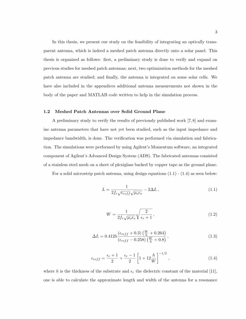
In this thesis, we present our study on the feasibility of integrating an optically trans-

parent antenna, which is indeed a meshed patch antenna directly onto a solar panel. This

thesis is organized as follows: first, a preliminary study is done to verify and expand on

previous studies for meshed patch antennas; next, two optimization methods for the meshed

patch antenna are studied; and finally, the antenna is integrated on some solar cells. We

have also included in the appendices additional antenna measurements not shown in the

body of the paper and MATLAB code written to help in the simulation process.

1.2 Meshed Patch Antennas over Solid Ground Plane

A preliminary study to verify the results of previously published work [7,8] and exam-

ine antenna parameters that have not yet been studied, such as the input impedance and

impedance bandwidth, is done. The verification was performed via simulation and fabrica-

tion. The simulations were performed by using Agilent’s Momentum software, an integrated

component of Agilent’s Advanced Design System (ADS). The fabricated antennas consisted

of a stainless steel mesh on a sheet of plexiglass backed by copper tape as the ground plane.

For a solid microstrip patch antenna, using design equations (1.1) - (1.4) as seen below:

L =1

2fr√εreff

√µoεo

− 2∆L , (1.1)

W =1

2fr√µoεo

√2

εr + 1, (1.2)

∆L = 0.412h(εreff + 0.3)

(Wh + 0.264

)(εreff − 0.258)

(Wh + 0.8

) , (1.3)

εreff =εr + 1

2+εr − 1

2

[1 + 12

h

W

]−1/2

, (1.4)

where h is the thickness of the substrate and εr the dielectric constant of the material [11],

one is able to calculate the approximate length and width of the antenna for a resonance

4

(a) (b)

(c)

Fig. 1.1: Layouts for momentum simulations all three have a length and width of 35.3 mmand 44.7 mm, respectively: (a) has a line width of 1.2 mm and a transparency of 27.91%;(b) has a line width of 1.0 mm and a transparency of 40.56%; (c) has a line width of 0.3mm and a transparency of 82.74%

of about 2.5 GHz. Also needed for the calculations is the material properties for plexiglass

obtained from Pozar [12].

1.2.1 Meshed Patch Antenna Layouts

Once the length and width of a solid patch are determined, it is intended to investigate

the effect of how creating the patch out of a mesh changes the properties of the antenna.

Several meshed patches were drawn and simulated in Agilent’s Momentum software. To

minimize the number of variables, the length and width of all the antennas was the same.

A number of layouts are selected and presented in Fig. 1.1(a)–(c).

5

1.2.2 Feeding

There are mainly three feeding methods that can be conveniently implemented by

Agilent’s Momentum software in order to match the patch to the microstrip feed-line. The

three matching methods are: stub matching, quarter wave transformer, and inset feed. For

a solid patch antenna there are formulas [11] for any of the three matching methods. But

for a meshed patch antenna there is no such exact formula, and those for a solid patch

antenna are only approximate, so the process of creating an accurate matching network

is an iterative process. The process to calculate the input impedance of the meshed patch

antenna is described in section 1.2.3. After the input impedance of the antenna is calculated,

we can accordingly design the matching network.

1.2.3 Impedance Calculations

For the following descriptions, please refer to Fig. 1.1(a). The input impedance of

the meshed patch antenna is calculated by considering the antenna as the load (noted as

ZL) and by using the measured input impedance at the port (labeled A) and then forward

calculating to obtain the input impedance of the meshed patch (label C). This is done by

using the transmission line impedance equation [12]. Starting with:

Zin = ZoZL + jZotan(βl)Zo + jZLtan(βl)

, (1.5)

Zin is the measured input impedance at the port (labeled A) Zo and the quantity βl can be

calculated with the aid of the Line Calc tool in Agilent’s Advanced Design system (ADS).

This leaves ZL as the only unknown in the equation; therefore, solving equation (1.5) for

ZL one can obtain the following equation:

ZL = ZoZin − jZotan(βl)Zo − jZintan(βl)

. (1.6)

Using equation (1.6), the measured input impedance of the port (labeled A) and the dimen-

sions of the first section of the line feed, one obtains the approximate input impedance at

6

Fig. 1.2: Dimensions of meshed patch antenna.

the location labeled B. Using equation (1.6) again with the calculated input impedance at

the location labeled B and with the dimensions of the quarter wave transformer the input

impedance of the meshed patch is obtained. Redesigning the feed network with the specified

input impedance, the simulation is run again. This process is run for a maximum of three

times until the simulations S11 measurement at the resonant frequency is below -20 dB.

1.2.4 Momentum Simulations

In this work, the transparency of a patch is defined by the percentage of see-though

area on the patch as shown below:

Transparency =[1− Aconductor

Apatch

]· 100% =

q(NL+MW )− q2NMWL

· 100% , (1.7)

where q is the line width of the mesh, N is number of lines parallel to the width of the

patch, M is the number of lines parallel to the length of the patch, L is the length of the

patch, and W is the width of the patch (see Fig. 1.2).

7

Seven different meshed patch geometries were drawn of different optical transparencies

and simulated in Agilent’s Momentum software. Once a good feed network was found, sev-

eral antenna parameters were extracted. In Fig. 1.3(a) one can see that as the transparency

of the patch is increased the resonant frequency of the patch decreases. This introduces

the possibility of minimizing the antenna design because the physical length of the patch is

the main determining factor in the resonant frequency as noted by Clasen [7]. A possible

explanation is that creating the patch out of mesh increases the fringing fields; therefore,

increasing the electrical length [11] of the antenna. Also from Fig. 1.3(b) one is able

to see that increasing the transparency decreases the impedance bandwidth. Impedance

bandwidth is defined by the following equation:

BW =fh − fl

fr, (1.8)

where fh is the highest frequency at which the voltage standing wave ratio (VSWR) is

below 2, fl is the lowest frequency at which the VSWR is below 2, and fr is the frequency

of the minimum VSWR. Also as seen in Figs. 1.3(c), (d) both the gain and directivity of

the antennas degrades with the increasing transparency. Finally, from Fig. 1.3(e) it is seen

that the input impedance of the patch increases with the transparency of the patch.

1.3 Fabrication with Wire Mesh

To show the feasibility and possibility of fabrication, several meshed patch antennas

were fabricated with the use of a stainless steel wire mesh. Two different sizes of mesh were

used. The first one consisted of 0.4068 mm diameter wire with square gaps between each

wire having edges of 2.19 mm. The smaller mesh has wires with a diameter of 0.1524 mm

with square gaps of 1.56 mm. As seen in the momentum simulations, the input impedance

to the antenna is larger in comparison to a solid patch, see Fig. 1.3(e); therefore, it is not

very feasible to fabricate a quarter-wave transformer. For this reason, to match the feed to

the antenna with the possibility of tuning, either a tuning stub or probe feed is used.

8

(a) (b)

(c) (d)

(e) (f)

Fig. 1.3: Results from momentum simulations showing the effect of the mesh transparencyon some antenna parameters: (a) resonant frequency; (b) impedance bandwidth; (c) gain;(d) directivity; (e) input impedance; (f) antenna efficiency.

9

(a) (b)

Fig. 1.4: Fabricated stub tuned antennas: (a) Length of 45 mm and width of 50 mm,transparency of 71%; (b) Length of 41 mm and width of 50 mm, transparency of 82%.

1.3.1 Stub Tuning

Shown in Fig. 1.4 are the two meshed patches fabricated and tuned with a microstrip

stub matching technique. The meshed patch is connected to the copper feed line. Two

copper tapes between the mesh and the feed are placed above and below the patch to

assure a good of electrical connection. The stub was then varied in length and location to

obtain a good impedance match determined by measuring the S11 parameter at the resonant

frequency. More information on stub tuning can be found in a book by David Pozar [12].

The meshed patch antenna shown in Fig. 1.4(a) has a length of 45 mm and a width of 50

mm with an approximate transparency of 72%. While the patch shown in Fig. 1.4(b) has

a length and width of 41 mm and 50 mm, respectively.

The measured S11 results of the two meshed patch antennas obtained by using a network

analyzer are shown in Fig. 1.5. One aspect to take note of is that although the antenna

in Fig. 1.4(b), has a greater transparency; it has a bandwidth of 2.17%, while the antenna

with a lower transparency has a bandwidth of 1.77% (Fig. 1.4(a)). This is contrary to

the momentum simulation results obtained in section 1.2, where the results showed that

10

(a) (b)

Fig. 1.5: Fabricated stub tuned antennas measurments: (a) Length of 45 mm and width of50 mm, transparency of 71%; (b) Length of 41 mm and width of 50 mm, transparency of82%.

as the transparency of the antenna increased, the bandwidth of the patch is decreased.

These results implies the possibility that transparency is not the only factor of the antenna’s

performance, but that the geometry of the mesh is also a factor in the antenna functionality.

1.3.2 Probe Feed

Shown in Fig. 1.6 are two meshed patch antennas with coaxial probe feeds. The

antennas are built with the same wire mesh materials as those with the microstrip stub

feeding; therefore, they have the same transparencies of 71% and 82%. To achieve a good

electrical connection that stilled allowed the patch to move in relation to the probe to find

a good matching position, a small piece of copper tape was placed on top of the probe and

mesh to electrically connect the two as can also be seen in Fig. 1.6.

The S-Parameter measurements for the probe fed antennas are shown in Fig. 1.7. The

measured impedance bandwidth of the results in Fig. 1.7(a) is 3.1% while the measured

value shown in Fig. 1.7(b) is 6.9%. These results further confirm what we found when

using the sub feed where the impedance bandwidth can be increased by decreasing the line

width of the mesh geometry. It should be noted that decreasing the line width gives to an

11

(a) (b)

Fig. 1.6: Fabricated probe-fed antennas: (a) Length of 44 mm and width of 50 mm, trans-parency of 71%; (b) Length of 44 mm and width of 48.5 mm, transparency of 82%.

(a) (b)

Fig. 1.7: Fabricated probe-fed antennas measurements: (a) Length of 44 mm and width of50 mm, transparency of 71%; (b) Length of 44 mm and width of 48.5 mm, transparency of82%.

12

increase in transparency.

13

Chapter 2

Optimization of Meshed Patch Antennas

2.1 Optimization Via Line Width

The previous results from the patch antennas fabricated with wire mesh showed that

the transparency of the patch is not the only factor in the performance of the antenna. It is

seen that the antenna built from a finer wire grid has a greater bandwidth, although it has

a greater transparency compared with the antenna build with the thicker mesh. To further

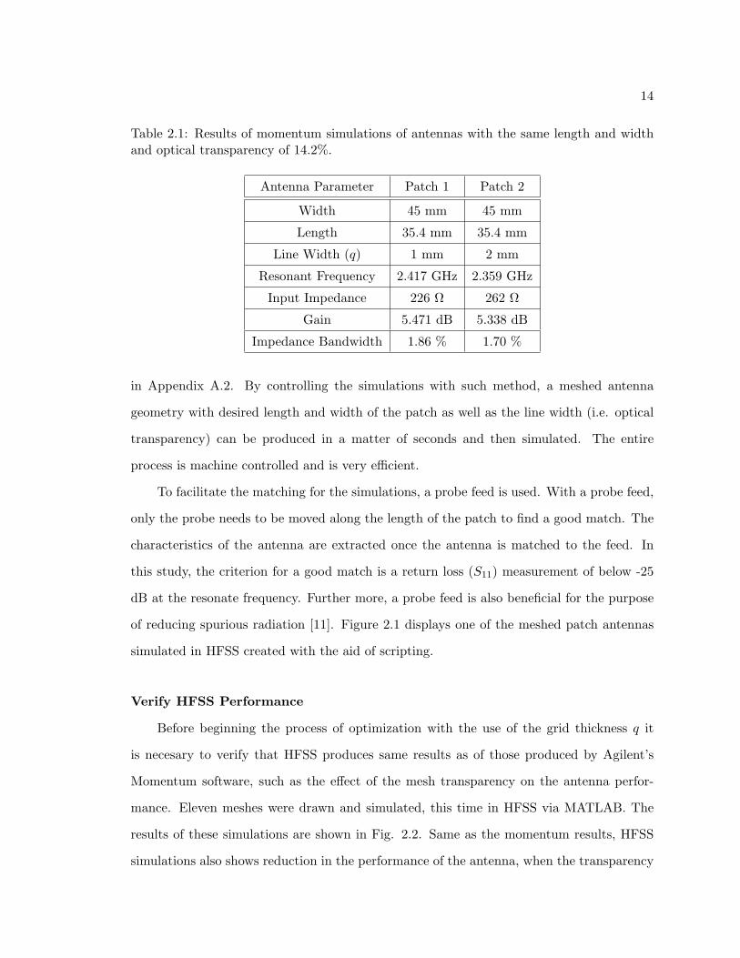
study the affect of the line width on antenna properties, two meshed patches having the

same transparency, but different line thickness q, see Fig. 1.2, were simulated with Agilent’s

Momentum software. Simulation results show that the patch with the thinner lines, q did

perform better in terms of gain and bandwidth. The results are summarized in Table 2.1.

It should be noted that in order to keep the transparency the same, the patch with the

smaller value of q must have more lines, hence the line density is greater. This observation

is consistant with Clasen that an antenna with greater line density performed better [7].

2.1.1 HFSS Simulation

The previous simulations are the results of only two meshed patch antennas. To verify

that the antennas performance improves with the decreasing line thickness q and to intro-

duce a method of optimizing the patch for transparency, more rigorous results are needed.

To limit the number of variables to only the line thickness, the antenna geometry must be

draw with precision. This process is tedious and time consuming if done with Agilent’s

Momentum software. Therefore Ansoft’s High Frequency Structural Simulator (HFSS) is

used and controlled with scripting files to initiate an automatic process. The scripts are

created and controlled by MATLAB. The MATLAB code used to create the scripts is seen

14

Table 2.1: Results of momentum simulations of antennas with the same length and widthand optical transparency of 14.2%.

Antenna Parameter Patch 1 Patch 2

Width 45 mm 45 mm

Length 35.4 mm 35.4 mm

Line Width (q) 1 mm 2 mm

Resonant Frequency 2.417 GHz 2.359 GHz

Input Impedance 226 Ω 262 Ω

Gain 5.471 dB 5.338 dB

Impedance Bandwidth 1.86 % 1.70 %

in Appendix A.2. By controlling the simulations with such method, a meshed antenna

geometry with desired length and width of the patch as well as the line width (i.e. optical

transparency) can be produced in a matter of seconds and then simulated. The entire

process is machine controlled and is very efficient.

To facilitate the matching for the simulations, a probe feed is used. With a probe feed,

only the probe needs to be moved along the length of the patch to find a good match. The

characteristics of the antenna are extracted once the antenna is matched to the feed. In

this study, the criterion for a good match is a return loss (S11) measurement of below -25

dB at the resonate frequency. Further more, a probe feed is also beneficial for the purpose

of reducing spurious radiation [11]. Figure 2.1 displays one of the meshed patch antennas

simulated in HFSS created with the aid of scripting.

Verify HFSS Performance

Before beginning the process of optimization with the use of the grid thickness q it

is necesary to verify that HFSS produces same results as of those produced by Agilent’s

Momentum software, such as the effect of the mesh transparency on the antenna perfor-

mance. Eleven meshes were drawn and simulated, this time in HFSS via MATLAB. The

results of these simulations are shown in Fig. 2.2. Same as the momentum results, HFSS

simulations also shows reduction in the performance of the antenna, when the transparency

15

Fig. 2.1: Example of a meshed patch antenna created via a scripting file for simulation.

is increased. For the simulations, all the antennas have length and width of 37 mm and

49 mm, respectively. The antenna substrates have a thickness of 2.032 mm with a relative

permittivity (εr) of 2.2.

An effect that was not captured in the momentum simulations, but can be studied by

HFSS is the input impedance as a function of distance from the edge of the patch. The

generally accepted equation for the input impedance as a function of distance from the edge

for a solid patch antenna is given by the following equation:

Rin(y) = Rin(y = 0)cos2(πLy), (2.1)

where Rin(y = 0) is the input impedance at the edge of the patch and L is the length of

the patch. To see if equation (2.1) is valid for a meshed patch antenna, several impedance

measurements were taken via simulations down the length of the patch. Figure 2.3 shows

the results as well as a line defined by equation (2.1). As seen, the simulated measurements

follow the prescribed equation. This shows that equation (2.1) is also valid for a meshed

patch antenna. The simulated patch had a line thickness q of 1.0 mm with a length and

width of 37 mm and 45 mm, respectively. The patch also had a transparency of 72.07%.

Line Width Effects

As mentioned previously, for these simulations, the length and width of the antennas

16

(a) (b)

(c) (d)

Fig. 2.2: Results from HFSS simulations - effects of transparency on the performance ofthe meshed antenna: (a) frequency, (b) impedance bandwidth, (c) peak gain, (d) radiationefficiency.

Fig. 2.3: HFSS simulation results showing the input impedance as a function of distance.Solid line is defined by equation (2.1) with an edge impedance value of 550 Ω.

17

(a) (b)

(c) (d)

Fig. 2.4: HFSS simulations results. All antennas have a transparency of 60.0% ±0.1% witha length and width of 37.0 mm and 45.0 mm, respectively. The solid lines are least-squaresfit to the data to help show the trend of the results.

are kept constant at 37.0 mm and 45.0 mm, respectively. The substrate of the antenna

is the same as previously mentioned. To see how the line width of the mesh affects the

performance of the antenna, the transparency of every meshed patch is fixed at 60.0% with

a deviation of ± 0.1% at a maximum. Therefore, in order to vary the line width of the grid

and keep the transparency constant, the number of grid lines parallel to the x and y axis

will change. Figure 2.4 has the results of the simulations.

It is seen from Figs. 2.4(a) - (c) that by decreasing the line thickness, the radiation

properties of the antenna are increasing. In comparison to the results shown in Fig. 2.2, it

can be seen that minimizing the line width of the mesh helps the meshed antenna perform

18

closer to that of a solid patch antenna. In other words, reducing the line thickness of the

mesh counteracts the effect of meshing the patch, or optimizes the meshed patch antenna

for performance. It is seen from Fig. 2.4(d) that the needed distance to insert the probe

feed is reduced. Referring to equation (2.1) it can be deduce that reducing the line thickness

of the mesh also decreases the input impedance of the antenna at the radiating edge.

Radiation Pattern and Cross-Polarization

We want to verify that the meshing of the patch does not significantly degrade the

radiation characteristics of the antenna. To verify this, we looked at both the radiation

patterns and cross polarization and compared those with that of a solid patch antenna. As

seen in Fig. 2.5, it is seen that the largest difference is in the cross-polarizations levels in

the H-plane reaching all the way up to just below -20 dB. On the other hand, in the E-plane

the shape changes, but the level of the cross-polarization does not increase significantly. As

shown in Fig. 2.6, there is no significant change in the radiations patterns from the solid

and meshed patch antennas. These results show that the meshing of the patch has little to

no effect on the co-polarized radiation and that the cross-polarized radiation stays below

an acceptable level. It should be noted that the meshed patch antenna for this study has a

line thickness of 2.28 mm.

2.1.2 Fabrication

To validate the simulated results, we conducted experiments by fabricating four differ-

ent meshed antennas. This is done by screen printing a silver-based conductive ink (created

by Creative Materials product number 124-46) onto a sheet of plexiglass. The plexiglass is

backed with copper tape to act as the ground plane for the antenna. It was designed to

fabricate all of the antennas with the same physical length, width, and optical transparency,

but due to the limits of the fabrication process there is some degree of inaccuracy. Table

2.2 shows the desired and actual dimensions of the patch antennas.

To account for not knowing the input impedance of the meshed patches, an insert feed

method was used to make it possible to tune the patch for a good impedance match. The

19

(a) (b)

(c) (d)

Fig. 2.5: Polarization levels. (a) H-Plane of a meshed patch antenna with a transparencyof 59.9%, (b) E-Plane for the meshed patch, (c) H-Plane for a solid patch, (d) E-Plane forthe solid patch.

20

(a) (b)

Fig. 2.6: Radiation patterns for both a solid and meshed patch antenna of the same physicaldimenstions. The meshed patch has an optical transparency of 59.9%, (a) is the meshedpatch, (b) is the solid patch.

process of finding a good match is to have the insert distance cut deeper than would be

expected, found via simulation, and then decrease the insert distance by adding copper

tape. One of the fabricated meshed patch antennas is shown in Fig. 2.7.

2.1.3 Measurements

S-Parameter Measurements

With the antennas build and matched, both the resonant frequency and impedance

bandwidth were measured with an HP 8510 Network analyzer. Two of the antennas S-

parameter measurements are shown in Fig. 2.8. The rest of the measurements of the other

antennas can be found in Appendix B.1 and seen in Figs. B.1 and B.2.

The measurements are summarized in Table 2.3. As seen in the table, the resonant

frequencies of the antenna increase with the decreasing of the line width. The bandwidth

does not have a clear pattern as the simulations do. This could be due to the discrepancies

in the fabrication of the line feeds and the matching which cannot be done to the precision

of a simulation. There also exists the noise when taking the measurements. Also as seen in

Table 2.3, the needed insert distance to match the line to the antenna has the overall trend

21

Fig. 2.7: Example of a fabricated meshed patch antenna that has been matched to the feedwith the insert feed method. Copper tape was used for the feed and for matching.

(a) (b)

Fig. 2.8: S-parameter measurements for two of the fabricated antennas, (a) is antenna 1a,and (b) is antenna 3b dimensions for both are found in Table 2.2.

22

Table 2.2: Fabricated antenna dimensions: line width effect. The measured dimensionswere done with a pair of electronic calipers. T is the optical transparency q, L, W, N, andM are the same as defined for equation (1.7).

Antenna Desired q (mm) Measured q (mm) L (mm) W (mm) N M T (%)

1a 0.3 0.3 36.85 44.84 20 24 69.69

1b 0.5 0.5 36.85 44.74 12 14 70.14

1c 0.81 0.8 36.85 44.67 7 9 70.04

1d 1.0 1.0 36.85 45.07 6 7 70.22

3b 1.49 1.5 36.72 45.06 4 5 69.17

solid - - 37.56 45.36 - - 0

Table 2.3: Fabricated antenna S-parameter measurements: line width.

Antenna Line Width (mm) Resonant Freq. (GHz) Bandwidth (%) Insert (mm)

1a 0.3 2.35 6.28 7.1

1b 0.5 2.275 3.65 6.3

1c 0.8 2.23 7.29 8.36

1d 1.0 2.2 7.58 8.17

3b 1.5 2.14 5.02 11.03

of increasing with the line width of the grid as was shown in the HFSS simulations.

Near-Field Measurements

The radiation characteristics of the antennas were measured with the NSI near-field

antenna range aligned for a spherical measurement. The set-up of the near-field range is

seen in Fig. B.3 in Appendix B.2. The directivity of the antennas and well as the co

and cross polarization levels are measured. All of the measurements are normalized by the

maximum radiation value of a solid rectangular patch antenna of the same length and width

as the mesh patch antennas. The solid patch antenna is also built on the same substrate as

the antennas of interest. This was done to compare the performance of the meshed antennas

with an antenna of well documented performance characteristics [11,13]. Only the radiation

characteristics of the front plane of the antenna are of interest and plotted. The back plain

23

(a) (b)

Fig. 2.9: Normalized radiation patterns for mesh patch 1a (values in dB), dimensions of thepatch can be seen in Table 2.2, (a) is the E-Plane, and (b) is the H-Plane. The solid line isthe co-polarized pattern and the dashed line is the cross-polarized pattern.

shows other affects that do not pertain to this paper, such as the finite ground plane effect

which is documented in another publication [14].

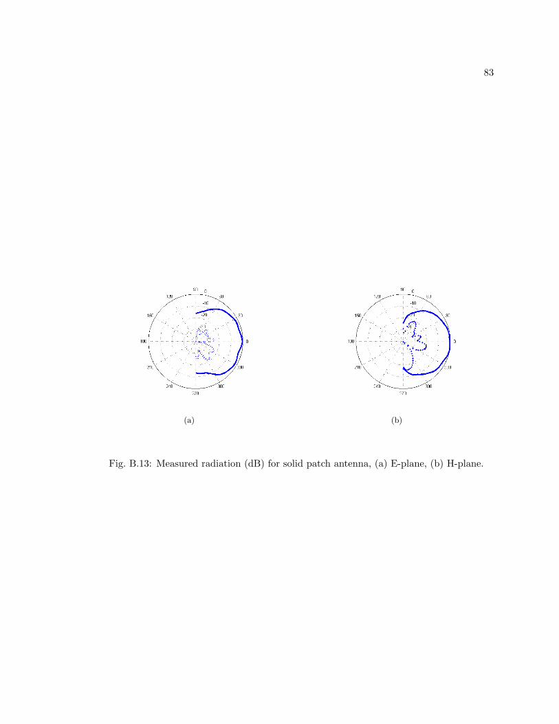
The measured radiation patterns for antennas 1a and 3b are shown in Figs. 2.9 and

2.10, respectively. Figure 2.11 shows the measured values of the solid patch used as the

standard. The other meshed antenna measurements can be seen in Appendix B.2 in Figs.

B.4 through B.13. As can be seen for both antennas the radiation in the H-Plane is as it

should be and other than the radiation intensity being lower than that of a solid patch,

there is little difference. The cross-polarization patterns are different, but still not above

-20 dB. One concern may be that even though the cross-polarizations levels are not greater

that those of the solid patch, the ratio of the cross-polarization to that of the co-polarization

is increased due to the lower levels in the co-polarization.

In the simulations, we studied the gain of the meshed patch antennas. A more reason-

able parameter for the experiment is the directivity, which is related to the gain as:

Go = εcdDo , (2.2)

where Go is the maximum gain, Do is the maximum directivity, and εcd is the antenna

24

(a) (b)

Fig. 2.10: Normalized radiation patterns for mesh patch 3b (values in dB), dimensions ofthe patch can be seen in Table 2.2, (a) is the E-Plane, and (b) is the H-Plane. The solidline is the co-polarized pattern and the dashed line is the cross-polarized pattern.

(a) (b)

Fig. 2.11: Normalized radiation patterns for a solid patch (values in dB), dimensions of thepatch can be seen in Table 2.2, (a) is the E-Plane, and (b) is the H-Plane. The solid line isthe co-polarized pattern and the dashed line is the cross-polarized pattern.

25

Fig. 2.12: Show the effect of the line width on the fabricated meshed patch antennas. Datais obtained from the near-field scanner.

efficiency. Shown in Fig. 2.12 is a plot showing the effect of the line width on the directivity

of the antenna. As can be seen the directivity of the antenna is increasing with the decreasing

line width as was similarly shown in the simulations with the gain with the exception of the

patch build with a line width of 1.5 mm. As for a comparison, it should be noted that the

solid patch antenna had a measured directivity of 8.55 dB.

2.1.4 Conclusions

It has been seen in both the simulations and measurements that the effect of the

meshed grids on the antenna performance. It is seen clearly in both the simulations and

measurements that the resonant frequency of the antenna increases with the decreasing

line width and that the input impedance decreases. In the HFSS simulations it was shown

that the impedance bandwidth of the antenna increases with the decreasing line width,

but the fabricated results were inconclusive due to the precision in fabrication. Also in the

simulations, it is seen that the decreasing line width helps maximize the gain of the antennas.

By comparison, it was also shown with the fabricated antennas that the directivity of the

antenna can be increased with minimizing the line width of the grid. Finally, the radiation

patterns of the meshed antennas are significantly affected by the meshed geometry in both

the simulations and measured results. Therefore, it can be concluded that by minimizing

the line width of the grid on the meshed patch antenna can be used to optimize the antenna

26

performance for a given optical transparency.

2.2 Optimization Via Orthogonal Lines

Presented in this section is another method to optimize the meshed patch antenna for

optical transparency and radiation properties. As mentioned by Wu, the possibility exits

of using only wires parallel to the length of the patch in place of a grid to optimize for

optical transparency [9]. In addition, as noted by Wu, the amount of current flowing on the

wires orthogonal to the length of the patch is minimal in comparison to the current on the

wires parallel to the length of the patch. For these reasons, it is our objective to optimize

the optical transparency by minimizing the number of lines orthogonal to the length of the

patch. We show the feasibility of this optimization through both simulations in HFSS and

fabrication and testing of antennas.

2.2.1 HFSS Simulation

For the simulated results, the line width for every patch is held constant at 0.85 mm.

The length and width of the patch are also held constant at 37.5 mm and 49.3 mm, respec-

tively. Additionally, the number of lines parallel to the length of the patch is the same for

each patch antenna, each has 15 lines. The number of lines orthogonal to the length of the

patch is then varied from 4 to 15. The simulation results performed in HFSS are shown in

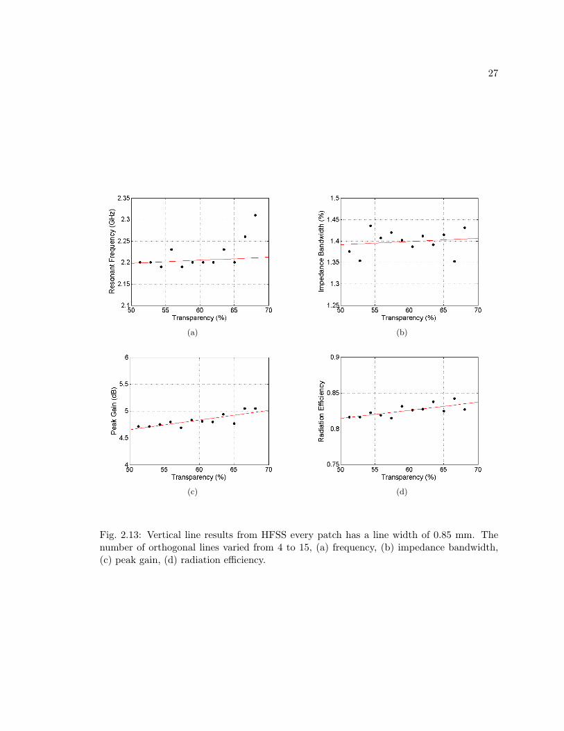
Fig. 2.13. As can be seen in Fig. 2.13(a) there is little effect on the resonant frequency

until the number of orthogonal lines has been reduce to 5 and below and the effect is still

minimal. For the other parameters such as the bandwidth, radiation efficiency and gain

there is no significant effect due to the vertical grid. These simulation results show that

optical transparency can be optimized without degrading the antenna performance.

Shown in Figs. 2.14 and 2.15 are the simulated radiation characteristics of two anten-

nas. One antenna has four orthogonal lines and the other one has 15 orthogonal lines. The

simulations show that there is no adverse affect in the radiation by reducing the number

of orthogonal lines. One effect that is seen by reducing the lines is the cross polarization

in the H-plane is reduced. This makes sense due to the fact that there are fewer lines for

27

(a) (b)

(c) (d)

Fig. 2.13: Vertical line results from HFSS every patch has a line width of 0.85 mm. Thenumber of orthogonal lines varied from 4 to 15, (a) frequency, (b) impedance bandwidth,(c) peak gain, (d) radiation efficiency.

28

(a) (b)

Fig. 2.14: HFSS simulated cross and co-polarization levels in dB. Cross polarization levelsare lower in magnitude. This antenna is feed by a coaxial probe and has four vertical lines,(a) is the E-plane, and (b) is the H-plane.

(a) (b)

Fig. 2.15: HFSS simulated cross and co-polarization levels in dB. Cross polarization levelsare lower in magnitude. This antenna is feed by a coaxial probe and has 15 vertical lines,(a) is the E-plane, and (b) is the H-plane.

29

Table 2.4: Fabricated antenna dimensions: vertical line effect: T is the optical transparencyq, L, W, N, and M are the same as defined for equation (1.7).

Antenna Desired q (mm) Measured q (mm) L (mm) W (mm) N M T (%)

2b 0.3 0.3 36.72 45.12 6 24 77.19

2c 0.3 0.3 36.76 45.0 4 24 78.27

3a 0.3 0.3 36.81 45.08 11 24 74.55

1a 0.3 0.3 36.85 44.84 20 24 69.69

solid - - 37.56 45.36 - - 0

current to flow down in the y-direction, hence less cross polarization in the H-plane.

2.2.2 Fabrication and Measurements

To verify the simulation results, four meshed antennas were fabricated and measured.

These antennas were also screen printed onto a sheet of plastic with a thickness of 2.032

mm and backed with copper tape for the ground plane. Table 2.4 shows the dimensions and

physical characteristics for each of the meshed antennas for this experiment set. Each of the

antennas has 24 lines parallel to the length of the patch. The number of lines orthogonal to

the length of the patch varies from 4 to 20, hence causing the optical transparency to vary

from 69.69% to 78.27%.

It is interesting to notice that in Fig. 2.16, when the number of orthogonal lines is

reduced, the antenna seems to have two resonant frequencies close to each other. With this

effect, that bandwidth of these antennas is higher than those in the previous experiment

which can be seen by comparing the results in Fig. 2.17(b) and table 2.3. The simulation

results show that there is not much change in the resonant frequency until the number of

orthogonal lines is at or below five. While with the fabricated patches the antenna with

four orthogonal lines is not much different from the one with 20 lines and the antenna with

six lines has a much higher resonant frequency than the other measured antennas. This can

be seen in Fig. 2.17(a).

Figures 2.18 and 2.19 are the radiation patterns for two fabricated antennas. The

30

(a) (b)

Fig. 2.16: S-parameter measurements for two of the fabricated antennas, (a) is antenna 2b,and (b) is antenna 2c dimensions for both are found in Table 2.4.

E-Plane for antenna 2b does not have the type of radiation pattern expected. This could

be associated with the phenomenon seen in the s-parameter measurements of this antenna.

For this reason, it is suggested not to reduce the number a orthogonal lines as low as 4 or

6. It can also be seen in Fig. 2.18 that antenna 2b has cross-polarization levels higher than

-20 dB. As seen in Fig. 2.19, the radiation pattern for antenna 3a is reasonable good other

than the E-plane has some distortion.

2.2.3 Conclusions

The simulations show that most of the current flows down the lines in the grid parallel

to the length of the patch. With this in mind, it was shown that the reduction of the lines

orthogonal to the length of the meshed patch is able to increase the optical transparency

without hindrance to the performance of the antenna. The reason for this is due to the

fact that there is minimal current flow on the orthogonal lines. Hence, another method of

optimizing the meshed patch antenna was demonstrated.

31

(a) (b)

(c) (d)

Fig. 2.17: Measured results for the reduction of the orthogonal lines, (a) resonant frequency,(b) impedance bandwidth, (c) directivity, (d) feed insert distance.

32

(a) (b)

Fig. 2.18: Normalized radiation patterns for mesh patch 2b (values in dB), dimensions ofthe patch can be seen in Table 2.4, (a) is the E-Plane, and (b) is the H-Plane. The solidline is the co-polarized pattern and the dashed line is the cross-polarized pattern.

(a) (b)

Fig. 2.19: Normalized radiation patterns for mesh patch 3a (values in dB), dimensions ofthe patch can be seen in Table 2.4, (a) is the E-Plane, and (b) is the H-Plane. The solidline is the co-polarized pattern and the dashed line is the cross-polarized pattern.

33

Chapter 3

Integration of Meshed Patch Antennas with Solar Cells

In the previous chapters, we have introduced meshed patch antennas, and methods

to optimize their radiation and optical properties. In this chapter, we concentrate on

integrating those transparent antennas on a solar panel. For such, a feeding method needs

to be chosen and the effects of the solar cells with antenna need to be determined. The

geometry of the proposed integration is shown in Fig. 3.1.

3.1 Feeding

A very important factor for the integration of the solar cells and the patch antenna is

the feeding method for the antenna. Throughout the process of optimizing the design of

the antenna the feed methods of a coaxial probe and inset feed method have been used in

simulation and fabrication, but these may not be the best methods to use. The inset feed

method has known problems for creating spurious radiation and limiting the bandwidth of

the antenna. Although the coaxial probe method reduces the spurious radiation to a certain

level, it also has a narrow bandwidth. Another disadvantage to both of these feed methods

is that both can create cross-polarized radiation which has been seen in the fabricated

antenna measurements [11].

Other possible feed methods to help the antenna performance have the feed mechanism

coupled to the antenna either via a gap or aperture [11]. These methods have the advantage

Fig. 3.1: Geometry of the proposed solar cell antenna.

34

of having the feed and other devices connected to the feed being isolated from the antenna.

One such method proposed is a modified inset feed [15]. This method is very similar to

the typical inset feed method, but instead of having the microstrip line connected directly

to the antenna, the feed is coupled though a small gap. This method has shown to have

good radiation characteristics and good cross-polarizations levels. A disadvantage is that

the feed is still on the top of the solar cells and will reduce the amount of light going in the

solar cell.

One solution to this light blocking problem is to have the feeding network placed on a

different layer and couple the feed to the antenna though an aperture. One such method

is a co-planar waveguide (CPW) coupled with a cross slot [16]. This method has the main

advantages of very low cross-polarization radiation and as with the previous method the

antenna and feeding network are isolated. One of the greatest advantages would be the

possibility of having the feeding network on the ground plane and not having it block any

sunlight needed for the solar cells. The one concern is how efficient the coupling though

the solar cells can be. The integrated solar cells and antenna proposed by Vaccaro had the

antenna coupled though an aperture, but the solar cells were placed on top of the antenna

so no coupling was done though the solar cells [2].

For simplicity and to have the results more comparable to the previous measured

results, an inset feed method was used when fabricating the solar cell antenna. This method

is easy to tune and match the antenna with the use of a copper tape. It may not be the best

choice for the final design, but for testing purposes it is a good and cost-friendly option.

3.2 Effect of Conductivity

Because it is difficult to know the exact material properties (such as the dielectric

constant and the conductivity) of the solar cells used to fabricate solar cell antennas, we

did several simulations to see the effects of the conductivity on the antenna performance.

Since the solar cells measured to be very thin, 0.15 mm, we expected the dielectric constant

not to be an important factor and we approximated it by the dielectric constant of silicon

at 11.9. This leaves only the conductivity of the solar cell level to vary.

35

The effect of the conductivity was done by simulating a meshed patch antenna in

HFSS on a two substrate layer. The antenna has a length and width of 37 mm and 45

mm, respectively with 11 parallel lines and nine orthogonal lines and a line width of 0.55

mm. This gives the antenna an optical transparency of 74.98%. The top dielectric layer

has a thickness of 2.032 mm and a dielectric constant of 2.6. The second layer also has a

thickness of 2.032 mm, a dielectric constant of 11.9 and the conductivity was varied from 0

S/m to 100 S/m to study the effect of conductivity of solar cells on antenna properties. The

reason for having the second layer not as thin as the measured solar cells is to speed up the

simulations. After we have the parametric study, we can simulate a solar cell with the exact

thickness, and to fabricate the antennas according to the simulations. Otherwise with such

a thin substrate, the mesh of the numerical analysis needs to be small hence increasing the

complexity of the simulations and take a long time.

Figure 3.2 shows the effect of the conductivity on the antenna. The effect on the

resonate frequency is very minimal and there is not clear pattern; therefore we did not

present those results. The highest resonate frequency is at 2.17 GHz and the lowest is at

2.14 GHz.

As seen in Fig. 3.2, once the conductivity of the layer is above 20 S/m there is little

change in the antenna properties. A possible explanation is that once the conductivity high

enough, the solar cell layer is acting as part of the ground plane. So instead of having a

two layer substrate, it is as if there is only one layer and a thick ground plane. Figures

3.2(c) and (e) suggest when the conductivity of the layer below 1 S/m, the solar layer is

creating losses and hence decreasing the gain and efficiency of the antenna. This would

also increase the bandwidth as seen. This is due to how the bandwidth is calculated from

the S11. An added electrical loss in the substrate decreases the return loss hence a greater

impedance bandwidth. Overall, it can be seen that if the conductivity of the solar cells is

great enough there will be little effect on the antenna performance. On the other hand, if

the conductivity is below 1 S/m the performance will be hindered.

36

(a) (b)

(c) (d)

(e) (f)

Fig. 3.2: Effect of conductivity on the antenna performance, (a) bandwith, (c) peak gain,(e) radiation efficiency, with the conductivity varied from 0 to 1 (S/m). For the effect ofthe conductivity for the (b) bandwith, (d) peak gain, (f) and radiation efficiency, with theconductivity varied from 10 ... 100 (S/m).

37

3.3 Fabrication

To test the meshed patch antenna integrated with solar cells a meshed patch antenna

was screen printed onto a PETG thermoplastic sheet having a thickness of 0.5 mm (this

thickness is to approximate a solar cell cover glass). The dielectric constant specified on

the data sheet is approximately 2.4 at 1 MHz. Solar cells were attached to an aluminum

sheet of metal with the use of a silver based conductive epoxy. The sheet of plastic with the

printed antenna was attached to the aluminum sheet with the use of nylon screws to hold

the assembly together. The antenna was fed with a microstrip feed line composed of copper

tape. It was originally desired to match the antenna to the feed via the inset method, but

this did not suceed, so a microstrip open circuit stub was used.

3.4 Measurments

Figure 3.3 shows the fabricated antenna before the impedance matching was completed

and the measured return loss after the impedance matching. The printed antenna has a

length and width of 37.14 mm and 44.91 mm, respectively, with a line width q of 0.46

mm. The antenna also has 24 parallel lines and four orthogonal lines with an optical

transparency of 71.68%. The antenna has a measured bandwidth of 32%. This can be

attributed to minimal number of orthogonal lines as seen in the results of section 2.2 and

the conductivity of the solar cells.

Figure 3.4 is a plot of the normalized radiation patterns for the antenna with the solar

cells. It should be noted that the pattern is normalized to the pattern of the solid patch

used in the previous section and the solid patch has a much thicker substrate. The measured

directivity of the antenna is 8.04 dB, but looking at the radiation intensity which is very

low and referring to equation (2.2) one can infer that the efficiency of the antenna is very

low. This is expected for the thin substrate used (0.5 mm). Also from the simulations, it

was seen that the conductivity of the solar cells reduces the efficiency of the antenna. It is

also shown by Fig. 3.4 that the cross-polarization levels in the H-plane are almost and at

some angles higher than the co-polarization levels.

38

(a) (b)

Fig. 3.3: Fabricated solar cell antenna, (a) is the fabricated antenna, (b) is the measuredS-parameters for the antenna.

(a) (b)

Fig. 3.4: Measured radiation plots for the solar cell antenna normalized with the solidpatch values are in dB. Solid lines are the co-polarization and the dashed lines are thecross-polarization, (a) is the E-Plane, and (b) is the H-Plane.

39

Chapter 4

Conclusions

This work shows the feasibility of integrating an optically transparent antenna directly

on the solar cell of a small satellite. We have shown the preliminary study and the optimiza-

tion of the meshed patch antenna for optical transparency and antenna performance. The

first method of optimization is the refining the line width of the mesh. This method showed

that by minimizing the line width of the grid, the performance of the antenna is enhanced

when the optical transparency of the patch was held constant. This was shown with the

aid of HFSS simulations and supported with the fabrication and measurement of printed

meshed patch antennas. The next optimization method shown was to reduce the number

of lines orthogonal to the length of the patch. In simulations with HFSS it is shown that

by reducing the orthogonal lines, the optical transparency of the patch is increased while

the performance of the antenna is not hindered. Simulations also show that the second

optimization method was also able to reduce the cross-polarization radiation. Finally, a

printed meshed antenna was integrated with solar cells and measured. It is seen that it is

feasible to integrate a meshed patch antenna with solar cells, but it was not very efficient

radiator at the current configuration.

For future work, it would be very beneficial to fabricate and test more antennas and try

different feeding methods, especially the CPW. This feeding configuration does not block

the sunlight for the solar cells and will produce better radiation characteristics. It is also

important to see how well the coupling can be though the solar cells and to see if special

solar cells need to be custom made. Methods are needed to counteract the reduction of

radiation efficiency caused by such thin substrate like the current cover glass used on solar

cells. In addition, it will be needed to do studies on the variation of the dielectric constant

due to temperature changes that will be experienced in space. Finally, other methods of

40

optimization can be studied. For example, the geometry of the meshed patch antenna does

not need to stay as a grid, so optimization tools such as the genetic algorithm can be used

to find an optimal geometry for optical transparency and antenna performance.

41

References

[1] “Small satellite home page,” [http://centaur.sstl.co.uk/SSHP/].

[2] S. Vaccaro, P. Torres, J. Mosig, A. Shah, J. Zurcher, A. Skrivervik, F. Gardiol,P. Maagt, and L. Gerlach, “Integrated solar panel antennas,” Electronic Letters, vol. 36,pp. 390–391, 2000.

[3] S. Vaccaro, P. Torres, J. Mosig, A. Shah, J.-F. Zurcher, A. Shrivervik, P. de Maagt,and L. Gerlach, “Stainless steel slot antenna with integrated solar cells,” ElectronicLetters, vol. 36, pp. 2059–2060, 2000.

[4] R. N. Simons and R. Q. Lee, “Feasibility study of optically transparent microstrippatch antenna,” NASA Technical Memorandum 107434.

[5] C. Mias, C. Tsakonas, N. Prountzos, D. Koutsogerogis, S. Liew, C. Oswald, R. Ranson,W. Cranton, and C. Thomas, “Optically transparent microstrip antennas,” in Antennasfor Automotives (Ref. No. 2000/002), IEE Colloquium on, pp. 8/1–8/6, 2000.

[6] N. Guan, H. Furuya, K. Himeno, K. Goto, and K. Ito, “A monopole antenna madeof a transparent conductive film,” in International Workshop on Antenna Technology:Small and Smart Antennas Metamaterials and Applications, IWAT ’07., pp. 263–266,2007.

[7] G. Clasen and R. Langley, “Meshed patch antennas,” IEEE Transactions on Antennasand Propagation, vol. 52, pp. 1412–1416, 2004.

[8] G. Clasen and R. Langley, “Gridded circular patch antennas,” Microwave and OpticalTechnology Letters, vol. 21, pp. 311–313, 1999.

[9] M.-S. Wu and K. Ito, “Basic study on see-though microstrip antennas constructed ona window glass,” in IEEE Transactions on Antennas and Propagation InternationalSymposium, pp. 499–502, July 1992.

[10] G. Clasen and R. Langley, “Meshed patch antenna integrated into car windshield,”Electronic Letters, vol. 36, pp. 781–782, 2000.

[11] C. A. Balanis, Antenna Theory Analysis and Design. Hoboken, NJ: John Wiley andSons, 2005.

[12] D. M. Pozar, Microwave Engineering. Hoboken, NJ: John Wiley and Sons, 2005.

[13] Y. Lo, D. Solomon, and W. Richards, “Theory and experiment on microstrip antennas,”IEEE Transactions on Antennas and Propagation, vol. 27, pp. 137–145, 1979.

[14] J. Huang, “The finite ground plane effect on the microstrip antenna radiation patterns,”IEEE Transactions on Antennas and Propagation, vol. 31, pp. 649–653, 1983.

42

[15] D. Jung, Y. Woo, and C. Ha, “Modified inset fed microstrip patch antenna,” in Asia-Pacific Microwave Conference, pp. 1346–1349, 2001.

[16] K. Hettak and G. Delisle, “A novel class of cpw coupled patch antenna for polariza-tion and frequency diversities,” in IEEE Transactions on Antennas and PropagationInternational Symposium, pp. 222–225, June 2002.

[17] K. R. Carver and J. W. Mink, “Microstrip antenna technology,” IEEE Transactionson Antennas and Propagation, vol. 29, pp. 2–24, 1981.

43

Appendices

44

Appendix A

HFSS Scripting

A.1 Simulation vs. Measurement

In previous chapters, we did not do a direct comparison of simulated antennas with

that of a measured antenna of the same physical properties. In this session, we present

the measured and simulated results of two meshed patch antennas. The antennas were

fabricated and measured and then simulated in HFSS. The only difference between the

simulation and fabricated antennas is that the inset distance for matching the feed and an-

tennas. The simulated antennas have a greater inset distance than the fabricated antennas.

The first patch has a length and width of 37.4 mm and 45.11 mm, respectively. The line

width was measured to be 1.04 mm with 9 lines orthogonal to the length of the patch and

11 lines parallel, and these measured parameters were used as inputs for the simulation.

Such geometry gives an optical transparency of 56%. Shown in Fig. A.1(a) is the com-

parison of the measured S-parameters and in Fig. A.2 is a comparison of the normalized

radiation patterns. The second patch has a length and width of 37.52 mm and 45.01 mm,

respectively. The line width of 1.23 mm with six orthogonal lines and seven parallel lines

with an optical transparency of 65%. The comparison of the measured and simulations for

the S-parameters and radiation patterns are shown in Figs. A.1(b) and A.3, respectively.

As can be seen, the simulations and measured results agree with each other very well.

One major difference in the radiation patterns is in the H-planes. In the simulations, at the

angles of ± 90 degrees, the radiation intensity approaches 0 while in the measured patterns

it does not approach 0. We also note a difference is the difference in the resonant frequencies

as seen in Fig. A.1. This is most likely due to not knowing the exact value of the dielectric

constant of the plastic (We used an approximate value for a plexiglass given by Pozar [12].).

45

(a) (b)

Fig. A.1: Measured vs. simulation comparison for the S11 measurements, (a) has an opticaltransparency of 56%, (b) has an optical transparency of 65%.

(a) (b)

Fig. A.2: Measured vs. simulation comparison for the radiation patterns of the first patch.Solid lines are the measured values and dashed lines are the simulated. Both are thenormalized dB patterns, (a) E-plane, (b) H-plane.

46

(a) (b)

Fig. A.3: Measured vs. simulation comparison for the radiation patterns of the secondpatch. Solid lines are the measured values and dashed lines are the simulated. Both are thenormalized dB patterns, (a) E-plane, (b) H-plane.

Carver points out that the shift in the resonant frequency is often caused by inadequate

knowledge of the dielectric constant [17]. Overall, the comparison shows that the simulation

and measured values are consistent.

A.2 MATLAB Code

Presented in this appendix is the MATLAB code written to create the scripting files.

The basic idea was to write the HFSS scripting commands to a file and then run the script.

The first set of code is the main set that was used to call the functions to start a project in

HFSS and then draw and simulate the antenna. The following are the main functions that

were used in creating the scripts.

function t = draw_run_patch(W,L,lines,q,units,insert,freq,sub,path,name)

h = sub(1);

er = sub(2);

tand = sub(3);

feedH = 5;

47

% Calculate a quarter Wavelength

quarter = (1/sqrt(8.854e-12*4*pi*1e-7))/(freq*1e9)/4;

% freq = [1.9,2.0,2.0 2.1 2.2 2.2];

% start = [1.85,1.94 1.99,2.07,2.13,2.16];

if strcmp(units,’cm’)

quarter = quarter * 100;

elseif strcmp(units, ’mm’)

quarter = quarter * 1000;

end

% create and run the HFSS script

solType = ’DrivenTerminal’;

% create of open the file for the script

fid = fopen([path,’drawPatch.vbs’],’w’);

% link to HFSS create project and name

startProject(path,name,solType,fid);

createMaterial(’sub’,er,1,0,tand,0,freq,fid);

% draw the substrate

sizeB = [2*quarter+W,2*quarter+L,h];

coord = [-quarter,-quarter,-h];

drawBox(sizeB,coord,’substrate’,’sub’,[0,128,255],.5,units,fid);

% draw the airBox

sizeB = [2*quarter+W,2*quarter+L,h+quarter];

48

coord = [-quarter,-quarter,-h];

drawBox(sizeB,coord,’Air’,’vacuum’,[234,234,234],.6,units,fid);

% draw the ground plane

sizeB = [2*quarter+W,2*quarter+L];

drawRec(sizeB,coord,’Z’,’GND_plane’,’vacuum’,[0,128,255],.3,units,fid);

% draw the coax feed of 50 ohms (air filled)

% createVarible(’offSet’,feedOff(i),’mm’,fid); % varible for position

xPos = W/2;

yPos = insert;

zPos = -(h+feedH);

coord = [xPos,yPos,zPos];

% draw the pin

sizeB = [0.7,(h+feedH)];

drawCyl(sizeB,coord,’Z’,’pin’,’copper’,0,[234,0,0],.4,units,fid);

% varCylCenter(’pin’,’offSet’,coord,units,’Y’,fid);

% draw the coax

sizeB = [1.6,feedH];

drawCyl(sizeB,coord,’Z’,’coax’,’vacuum’,1,[0,234,234],.4,units,fid);

% varCylCenter(’coax’,’offSet’,coord,units,’Y’,fid);

% draw the coax cover

sizeB = [1.7,feedH];

drawCyl(sizeB,coord,’Z’,’coax_cov’,’copper’,0,[0,234,234],.4,units,fid);

% varCylCenter(’coax_cov’,’offSet’,coord,units,’Y’,fid);

49

% Subtract the intersenting parts

subtract(’substrate’,’pin’,1,fid);

subtract(’GND_plane’,’coax_cov’,1,fid);

subtract(’coax_cov’,’coax’,1,fid);

subtract(’coax’,’pin’,1,fid);

subtract(’Air’,’pin’,1,fid);

% draw the wave port

radius = 1.7;

coord = [xPos,yPos,zPos];

drawCir(radius,coord,’Z’,’wavePort’,’vacuum’,[0,234,234],.4,units,fid);

% varCirCenter(’wavePort’,’offSet’,coord,units,’Y’,fid);

% Draw the Patch

t = DrawPatch4(W,L,lines,q, units,fid);

% create the boundaries and excitation

radiationBound(’Radiation’,’35,37,38,39,40’,fid);

assignFiniteCond(’Ground’,’GND_plane’,’copper’,fid)

assignFiniteCond(’patch1’,’patch’,’copper’,fid)

wavePortAssign(183,’coax_cov’,fid);

% Insert the farfield

farFieldSetup(’Far_Field’,[-180,180,10],[0,360,10],fid)

% Limit the mesh size in the Air box

meshLength(’Length1’,’Air’,quarter*4/10,’mm’,fid);

50

%setup the analyisis

analSet(’freq_sweep’,freq,40,fid);

analSweep(’freq_sweep’,’Sweep’,’Fast’,’LinearCount’,1,3,201,1,fid);

% run the analysis

fprintf(fid,’\noDesign.Analyze "freq_sweep"\n’);

closeProject(name,fid);

% close the script file

fclose(fid);

% run the sript

dos([’wscript ’, [path,’drawPatch.vbs’]]);

function out = DrawPatch4(W,L,lines,q, units,fid)

%--------------------------------------------------------------------------

% Description: Creates and runs the HFSS scriptfile to draw the patch and

% all of the geometry for the simulation

% Usage: out = DrawPatch(W,L,T,q, units,fid)

%

% Inputs: W = the width of the patch

% L = the Length of the pathc

% lines = (integer) the Desired number of parallel y lines

% q = the line width for the patch

% units = measurement units to use (m, cm, mm)

% fid = file identifier

%

% Outputs: out = ?

51

%--------------------------------------------------------------------------

% Calculate the number of lines

Ylines = lines(1);

Xlines = lines(2);

% round the number of lines to an integer

Xlines = round(Xlines); Ylines = round(Ylines);

% calculate the gap space

gapX = (W-Ylines*q)/(Ylines - 1);

gapY = (L - Xlines*q)/(Xlines -1);

% Calculate the true transparency

Tran = (gapX*gapY)*(Xlines-1)*(Ylines-1)/(W*L);

if Tran < 1

% draw the xlines

drawRec([W,q],[0,0,0],’Z’,’Xlines’,’vacuum’,[234,0,0],.3,units,fid);

duplicateLine(’Xlines’,[0,gapY+q,0],Xlines,units,fid);

% draw the ylines

drawRec([q,L],[0,0,0],’Z’,’Ylines’,’vacuum’,[234,0,0],.3,units,fid);

duplicateLine(’Ylines’,[gapX+q,0,0],Ylines,units,fid);

% unit the lines

% create the list of objects to unit

list = [’Xlines,’,’Ylines’];

52

for i = 1:Xlines-1

list = [list,[’,Xlines_’,sprintf(’%d’,i)]];

end

for i = 1:Ylines-1

list = [list,[’,Ylines_’,sprintf(’%d’,i)]];

end

unitObjects(list,’Xlines’,’patch’,fid);

else

Tran = 0;

drawRec([W,L],[0,0,0],’Z’,’patch’,’vacuum’,[234,0,0],.3,units,fid);

end

out = Tran;

Listed are the functions for drawing the shapes, setting up the analysis and other

necessary items scripts in HFSS. Functions are in alphabetic order.

function analSet(name,freq,maxPass,fid)

%--------------------------------------------------------------------------

% Description: add an anaylsis setup in HFSS

%

% Usage: analSet(name,freq,maxPass,fid)

%

% Inputs: name : string (name of the anaylsis)

% freq: float (solution frequency GHz)

% maxPass: int (maximum number of passes to find the solution)

% fid: file identifer

%--------------------------------------------------------------------------

53

freq = sprintf(’%0.4f’,freq);

maxPass = sprintf(’%d’,maxPass);

fprintf(fid,’\n’);

fprintf(fid,’REM --------- Set up an Analysis ------------------------\n’);

fprintf(fid,[’Set oModule = oDesign.GetModule("AnalysisSetup") \n’,...

’oModule.InsertSetup "HfssDriven", _\n’,...

’ Array("NAME:’,name,’", _\n’,...

’ "Frequency:=", "’,freq,’GHz", _\n’,...

’ "PortsOnly:=", false, _\n’,...

’ "MaxDeltaS:=", 0.02, _\n’,...

’ "UseMatrixConv:=", false, _\n’,...

’ "MaximumPasses:=", ’,maxPass,’, _\n’,...

’ "MinimumPasses:=", 1, _\n’,...

’ "MinimumConvergedPasses:=", 1, _\n’,...

’ "PercentRefinement:=", 30, _\n’,...

’ "BasisOrder:=", 1, _\n’,...

’ "UseIterativeSolver:=", false, _\n’,...

’ "DoLambdaRefine:=", true, _\n’,...

’ "DoMaterialLambda:=", true, _\n’,...

’ "SetLambdaTarget:=", false, _\n’,...

’ "Target:=", 0.3333, _\n’,...

’ "UseConvOutputVariable:=", false, _\n’,...

’ "IsEnabled:=", true, _\n’,...

’ "ExternalMesh:=", false, _\n’,...

’ "UseMaxTetIncrease:=", false, _\n’,...

’ "MaxTetIncrease:=", 100000, _\n’,...

’ "PortAccuracy:=", 2, _\n’,...

54

’ "UseABCOnPort:=", false, _\n’,...

’ "SetPortMinMaxTri:=", false)\n’]);

fprintf(fid,’REM -----------------------------------------------------\n’);

function analSweep(nameAnal,name,type,stepType,stat,finish,step,fields,fid)

%--------------------------------------------------------------------------

% Description: add a frequency sweep to an anaylsis in HFSS

%

% Usage:analSweep(nameAnal,name,type,stepType,start,finish,step,fields,fid)

%

% Inputs: nameAnal: string (name of the anaylsis to add the sweep to)

% name: string (name of the frequency sweep

% type: string (’Discrete’, ’Fast’, ’Interpolating’)

% stepType: string (’LinearStep’,’LinearCount’,’LogScale’)

% stat: float (starting frequency in GHz)

% finish: float (ending frequency in GHs)

% step: float (step size if ’LinearStep’ or the number of linear

% frequencies or the number of frequencies per decade)

% fields: int ( 0 to not save the fields, 1 to save the fields)

% fid: file identifer

%--------------------------------------------------------------------------

start = sprintf(’%0.4f’,start);

finish = sprintf(’%0.4f’,finish);

if strcmp(stepType,’LinearCount’)

step = sprintf(’%d’,step);

elseif strcmp(stepType,’LogScale’)

step = sprintf(’%d’,step);

else

55

step = sprintf(’%0.4f’,step);

end

fprintf(fid,’\n’);

fprintf(fid,’REM --------- Add a Frequency Sweep ---------------------\n’);

fprintf(fid,[’oModule.InsertFrequencySweep "’,nameAnal,’", _\n’,...

’ Array("NAME:’,name,’", "IsEnabled:=", true, _\n’,...

’ "SetupType:=", "’,stepType,’", _\n’,...

’ "StartValue:=", "’,start,’GHz", _\n’,...

’ "StopValue:=", "’,finish,’GHz", _\n’]);

if strcmp(stepType,’LinearStep’)

fprintf(fid,[’ "StepSize:=", "’,step,’GHz", _\n’,...

’ "Type:=", "’,type,’", _\n’]);

if fields == 0

fprintf(fid,’ "SaveFields:=", false, _\n’);

fprintf(fid,’ "ExtrapToDC:=", false)\n’);

else

fprintf(fid,’ "SaveFields:=", true, _\n’);

fprintf(fid,’ "ExtrapToDC:=", false)\n’);

end

end

if strcmp(stepType,’LinearCount’)

fprintf(fid,[’ "Count:=", ’,step,’, _\n’,...

’ "Type:=", "’,type,’", _\n’]);

if fields == 0

fprintf(fid,’ "SaveFields:=", false, _\n’);

fprintf(fid,’ "ExtrapToDC:=", false)\n’);

else

56

fprintf(fid,’ "SaveFields:=", true, _\n’);

fprintf(fid,’ "ExtrapToDC:=", false)\n’);

end

end

if strcmp(stepType,’LogScale’)

fprintf(fid,[’ "SamplesPerDecade:=", ’,step,’, _\n’,...

’ "Type:=", "’,type,’", _\n’]);

if fields == 0

fprintf(fid,’ "SaveFields:=", false, _\n’);

fprintf(fid,’ "ExtrapToDC:=", false)\n’);

else

fprintf(fid,’ "SaveFields:=", true, _\n’);

fprintf(fid,’ "ExtrapToDC:=", false)\n’);

end

else

%do nothing

end

fprintf(fid,’\nREM ---------------------------------------------------\n’);

function assignFiniteCond(nameBound,nameObj,material,fid)

%--------------------------------------------------------------------------

% Description: Assign an object a boundary condtion of a finite condutivity

%

% Usage: assignFiniteCond(nameBound,nameObj,material,fid)

%

% Inputs: nameBound = string (will be the name of the boundary)

% nameObj = string (name of the object to apply the boundary to)

% material = string (name of the material to use)

% fid = file identifier

57

%--------------------------------------------------------------------------

fprintf(fid,’\n’);

fprintf(fid,’REM --------- Create a Finit Cond. Boundary -------------\n’);

fprintf(fid,[’oModule.AssignFiniteCond Array("NAME:’,nameBound,’", _\n’,...

’ "Objects:=", Array("’, nameObj,’"), _\n’,...

’ "UseMaterial:=", true, _\n’,...

’ "Material:=", "’,material,’", _\n’,...

’ "Roughness:=", "0um", _\n’,...

’ "UseThicknss:=", false, _\n’,...

’ "InfGroundPlane:=", false) _\n’]);

fprintf(fid,’REM -----------------------------------------------------\n’);

function closeProject(name,fid)

%--------------------------------------------------------------------------

% Decription: save the project and close it

%

% Usage: closeProject(name,fid)

%

% Inputs: name: string (name of project to close

% fid: file identifier

%--------------------------------------------------------------------------

fprintf(fid,’\n\noProject.Save\n’);

fprintf(fid,[’oDesktop.CloseProject "’,name,’"’]);

function createMaterial(name,er,mu,sig,tand,mtand,freq,fid)

%--------------------------------------------------------------------------

% Desription: create a material to use in the HFSS project

%

58

% Useage: createMaterial(name,er,mu,sig,tand,mtand,freq)

%

% Inputs: name: string (name of material)

% er: permitivity of material

% mu: permability of material

% sig: condutivity of the material

% tand: dielectric loss tangent

% mtand: magnetic loss tangent

% freq: measured frequency

% fid: file identifier

%--------------------------------------------------------------------------

fprintf(fid,’\n’);

fprintf(fid,’REM --------- Create a Material -------------------------\n’);

fprintf(fid,’Set oDefinitionManager = oProject.GetDefinitionManager()\n’);

fprintf(fid,[’oDefinitionManager.AddMaterial Array("NAME:’,name,’", _\n’]);

fprintf(fid,[’ "CoordinateSystemType:=","Cartesian",’,...

’ Array("NAME:AttachedData"),_\n’]);

fprintf(fid, ’ Array("NAME:ModifierData"), _\n’);

fprintf(fid,[’ "permittivity:=","’,sprintf(’%0.4f’,er),’",_\n’]);

fprintf(fid,[’ "permeability:=","’,sprintf(’%0.4f’,mu),’",_\n’]);

fprintf(fid,[’ "conductivity:=","’,sprintf(’%0.4f’,sig),’",_\n’]);

fprintf(fid,[’ "dielectric_loss_tangent:=","’,sprintf(’%0.4f’,tand),...

’",_\n’]);

fprintf(fid,[’ "magnetic_loss_tangent:=","’,sprintf(’%0.4f’,mtand),...

’",_\n’]);

fprintf(fid,[’ "delta_H_freq:=","’,sprintf(’%0.0f’,round(freq)),’")\n’]);

fprintf(fid,’REM -----------------------------------------------------\n’);

function drawBox(sizeB,coord,name,material,color,T,units,fid)

59

%--------------------------------------------------------------------------

% Description: Write the Script to draw a box in HFSS

%

% Usage: drawBox(sizeB,coord,name,material,color,T,units,fid)

%

% Inputs: sizeB = 3x1 vector (x,y,z)

% coord = 3x1 vector (xcoord,ycoord,zcoord)

% name = string (name of box)

% material = string (name of matrial)

% color = 3x1 vector of (R,G,B)

% T = transparency of the box (i.e. 0.5)

% units = string (m,cm,mm)

% fid = file identifier

%--------------------------------------------------------------------------

% put the color in the correct format

color = [’(’,sprintf(’%d’,round(color(1))),’ ’,...

sprintf(’%d’,round(color(2))),’ ’,...

sprintf(’%d’,round(color(3))),’)’];

fprintf(fid,’\n’);

fprintf(fid,’REM --------- Draw a box---------------------------------\n’);

fprintf(fid,[’oEditor.CreateBox Array("NAME:BoxParameters",’,...

’ "CoordinateSystemID:=",-1,_\n’]);

fprintf(fid,[’ "XPosition:=","’,sprintf(’%0.4f’,coord(1)),’"&"’,...

units,’",_\n’]);

fprintf(fid,[’ "YPosition:=","’,sprintf(’%0.4f’,coord(2)),’"&"’,...

units,’",_\n’]);

fprintf(fid,[’ "ZPosition:=","’,sprintf(’%0.4f’,coord(3)),’"&"’,...

60

units,’",_\n’]);

fprintf(fid,[’ "XSize:=","’,sprintf(’%0.4f’,sizeB(1)),’"&"’,...

units,’",_\n’]);

fprintf(fid,[’ "YSize:=","’,sprintf(’%0.4f’,sizeB(2)),’"&"’,...

units,’",_\n’]);

fprintf(fid,[’ "ZSize:=","’,sprintf(’%0.4f’,sizeB(3)),’"&"’,...

units,’"),_\n’]);

fprintf(fid,[’ Array("NAME:Atrributes", "Name:=", "’,name,...

’", "Flags:=","",_\n’]);

fprintf(fid,[’ "Color:=", "’,color,’", "Transparency:=",’,...

sprintf(’%0.4f’,T),’,_\n’]);

fprintf(fid,’ "PartCoordinateSystem:=", "Global",_\n’);

fprintf(fid,[’ "MaterialName:=", "’,material, ’", _\n’]);

fprintf(fid,’ "SolveInside:=", true)\n’);

fprintf(fid,’REM -----------------------------------------------------\n’);

function drawCir(radius,coord,axis,name,material,color,T,units,fid)

%--------------------------------------------------------------------------

% Description: Write the Script to draw a circle in HFSS

%

% Usage: drawCir(radius,coord,axis,name,material,color,T,units,fid)

%

% Inputs: radius = 1x1 vector (radius)

% coord = 3x1 vector (xcoord,ycoord,zcoord)

% axis = string (axis parallel to circle i.e. ’X’,’Y’,’Z’)

% name = string (name of box)

% material = string (name of matrial)

% color = 3x1 vector of (R,G,B)

% T = transparency of the box (i.e. 0.5)

61

% units = string (m,cm,mm)

% fid = file identifier

%

% Notes on axis with relation to size

% Axis sizeB(1) sizeB(2)

% X y z

% Y z x

% Z x y

%--------------------------------------------------------------------------

% put the color in the correct format

color = [’(’,sprintf(’%d’,round(color(1))),’ ’,...

sprintf(’%d’,round(color(2))),’ ’,...

sprintf(’%d’,round(color(3))),’)’];

fprintf(fid,’\n’);

fprintf(fid,’REM --------- Draw a Rectangle---------------------------\n’);

fprintf(fid,[’oEditor.CreateCircle Array("NAME:CircleParameters",’,...

’ "CoordinateSystemID:=",-1,_\n’]);

fprintf(fid, ’ "IsCovered:=", true, _\n’);

fprintf(fid,[’ "XCenter:=","’,sprintf(’%0.4f’,coord(1)),’"&"’,...

units,’",_\n’]);

fprintf(fid,[’ "YCenter:=","’,sprintf(’%0.4f’,coord(2)),’"&"’,...

units,’",_\n’]);

fprintf(fid,[’ "ZCenter:=","’,sprintf(’%0.4f’,coord(3)),’"&"’,...

units,’",_\n’]);

fprintf(fid,[’ "Radius:=","’,sprintf(’%0.4f’,radius),’"&"’,...

units,’",_\n’]);

62

fprintf(fid,[’ "WhichAxis:=","’,axis,’"),_\n’]);

fprintf(fid,[’ Array("NAME:Atrributes", "Name:=", "’,name,...

’", "Flags:=","",_\n’]);

fprintf(fid,[’ "Color:=", "’,color,’", "Transparency:=",’,...

sprintf(’%0.4f’,T),’,_\n’]);

fprintf(fid,’ "PartCoordinateSystem:=", "Global",_\n’);

fprintf(fid,[’ "MaterialName:=", "’,material, ’", _\n’]);

fprintf(fid,’ "SolveInside:=", true)\n’);

fprintf(fid,’REM -----------------------------------------------------\n’);

function drawCyl(sizeB,coord,axis,name,material,inside,color,T,units,fid)

%--------------------------------------------------------------------------

% Description: Write the Script to draw a cylinder in HFSS

%

% Usage: drawCyl(sizeB,coord,axis,name,material,inside,color,T,units,fid)

%

% Inputs: sizeB = 2x1 vector (radius, heigth)

% coord = 3x1 vector (xcoord,ycoord,zcoord) of the center

% axis = string (’X’, ’Y’, ’Z’)

% name = string (name of box)

% material = string (name of matrial)

% inside = 0 no solve inside 1 = solve inside

% color = 3x1 vector of (R,G,B)

% T = transparency of the box (i.e. 0.5)

% units = string (m,cm,mm)

% fid = file identifier

%--------------------------------------------------------------------------

% put the color in the correct format

63

color = [’(’,sprintf(’%d’,round(color(1))),’ ’,...

sprintf(’%d’,round(color(2))),’ ’,...

sprintf(’%d’,round(color(3))),’)’];

fprintf(fid,’\n’);

fprintf(fid,’REM --------- Draw a Cyliner ----------------------------\n’);

fprintf(fid,[’oEditor.CreateCylinder Array("NAME:BoxParameters",’,...

’ "CoordinateSystemID:=",-1,_\n’]);

fprintf(fid,[’ "XCenter:=","’,sprintf(’%0.4f’,coord(1)),’"&"’,...

units,’",_\n’]);

fprintf(fid,[’ "YCenter:=","’,sprintf(’%0.4f’,coord(2)),’"&"’,...

units,’",_\n’]);

fprintf(fid,[’ "ZCenter:=","’,sprintf(’%0.4f’,coord(3)),’"&"’,...

units,’",_\n’]);

fprintf(fid,[’ "Radius:=","’,sprintf(’%0.4f’,sizeB(1)),’"&"’,...

units,’",_\n’]);

fprintf(fid,[’ "Height:=","’,sprintf(’%0.4f’,sizeB(2)),’"&"’,...

units,’",_\n’]);

fprintf(fid,[’ "WhichAxis:=","’,axis,’"),_\n’]);

fprintf(fid,[’ Array("NAME:Atrributes", "Name:=", "’,name,...

’", "Flags:=","",_\n’]);

fprintf(fid,[’ "Color:=", "’,color,’", "Transparency:=",’,...

sprintf(’%0.4f’,T),’,_\n’]);

fprintf(fid,’ "PartCoordinateSystem:=", "Global",_\n’);

fprintf(fid,[’ "MaterialName:=", "’,material, ’", _\n’]);

if inside == 0

fprintf(fid,’ "SolveInside:=", false)\n’);

else

fprintf(fid,’ "SolveInside:=", true)\n’);

64

end

fprintf(fid,’REM -----------------------------------------------------\n’);

function drawRec(sizeB,coord,axis,name,material,color,T,units,fid)

%--------------------------------------------------------------------------

% Description: Write the Script to draw a rectangle in HFSS

%

% Usage: drawRec(sizeB,coord,axis,name,material,color,T,units,fid)

%

% Inputs: sizeB = 2x1 vector (W,L)

% coord = 3x1 vector (xcoord,ycoord,zcoord)

% axis = string (axis parallel to rectangle i.e. ’X’,’Y’,’Z’)

% name = string (name of box)

% material = string (name of matrial)

% color = 3x1 vector of (R,G,B)

% T = transparency of the box (i.e. 0.5)

% units = string (m,cm,mm)

% fid = file identifier

%

% Notes on axis with relation to size

% Axis sizeB(1) sizeB(2)

% X y z

% Y z x

% Z x y

%--------------------------------------------------------------------------

% put the color in the correct format

color = [’(’,sprintf(’%d’,round(color(1))),’ ’,...

sprintf(’%d’,round(color(2))),’ ’,...

65

sprintf(’%d’,round(color(3))),’)’];

fprintf(fid,’\n’);

fprintf(fid,’REM --------- Draw a Rectangle---------------------------\n’);

fprintf(fid,[’oEditor.CreateRectangle Array("NAME:BoxParameters",’,...

’ "CoordinateSystemID:=",-1,_\n’]);

fprintf(fid, ’ "IsCovered:=", true, _\n’);

fprintf(fid,[’ "XStart:=","’,sprintf(’%0.4f’,coord(1)),’"&"’,...

units,’",_\n’]);

fprintf(fid,[’ "YStart:=","’,sprintf(’%0.4f’,coord(2)),’"&"’,...

units,’",_\n’]);

fprintf(fid,[’ "ZStart:=","’,sprintf(’%0.4f’,coord(3)),’"&"’,...

units,’",_\n’]);

fprintf(fid,[’ "Width:=","’,sprintf(’%0.4f’,sizeB(1)),’"&"’,...

units,’",_\n’]);

fprintf(fid,[’ "Height:=","’,sprintf(’%0.4f’,sizeB(2)),’"&"’,...

units,’",_\n’]);

fprintf(fid,[’ "WhichAxis:=","’,axis,’"),_\n’]);

fprintf(fid,[’ Array("NAME:Atrributes", "Name:=", "’,name,...

’", "Flags:=","",_\n’]);

fprintf(fid,[’ "Color:=", "’,color,’", "Transparency:=",’,...

sprintf(’%0.4f’,T),’,_\n’]);

fprintf(fid,’ "PartCoordinateSystem:=", "Global",_\n’);

fprintf(fid,[’ "MaterialName:=", "’,material, ’", _\n’]);

fprintf(fid,’ "SolveInside:=", true)\n’);

fprintf(fid,’REM -----------------------------------------------------\n’);

function duplicateLine(name, offset,number,units,fid)

%--------------------------------------------------------------------------

66

% Description: duplicate an object along a line

%

% Usage: duplicateLine(name, offset,number,units,fid)

%

% Inputs: name: string (name of object to duplicate)

% offest: 3x1 vector (x,y,z) distance to duplicate from where the

% object was started to be drawn

% number: number of object to make

% units: string (m,cm,mm)

% fid: file identifier

%

% Note of clones names: the clones will be names ’name_1’ where 1 increment

% for each new clone

%--------------------------------------------------------------------------

fprintf(fid,’\n’);

fprintf(fid,’REM --------- Duplicate an object -----------------------\n’);

fprintf(fid,[’oEditor.DuplicateAlongLine Array("NAME:Selections",’,...

’ "Selections:=", _\n’]);

fprintf(fid,[’ "’,name,...

’"), Array("NAME:DuplicateToAlongLineParameters", _\n’]);

fprintf(fid,[’ "CoordinateSystemID:=", -1, "CreateNewObjects:=",’,...

’ true, _\n’]);

fprintf(fid,[’ "XComponent:=","’,sprintf(’%0.4f’,offset(1)),’"&"’,...

units,’",_\n’]);

fprintf(fid,[’ "YComponent:=","’,sprintf(’%0.4f’,offset(2)),’"&"’,...

units,’",_\n’]);

fprintf(fid,[’ "ZComponent:=","’,sprintf(’%0.4f’,offset(3)),’"&"’,...

67

units,’",_\n’]);

fprintf(fid,[’ "NumClones:=","’,sprintf(’%0.0f’,number),’"), _\n’]);

fprintf(fid,’ Array("NAME:Options", "DuplicateBoundaries:=", false)\n’);

fprintf(fid,’REM -----------------------------------------------------\n’);

function farFieldSetup(name,theta,phi,fid)

%--------------------------------------------------------------------------

% Description: Setup a farField Radiation Setup in HFSS

%

% Usage: farFieldSetup(name,theta,phi,fid)

%

% Inputs: name = string (name of the farfield sphere)

% theta = 3x1 vector ([thetaStart,thetaStop,thetaStep] degrees)

% phi = 3x1 vector ([phiStart,phiStop,phiStep] degrees);

% fid = file indetidifer

%--------------------------------------------------------------------------

phi1 = sprintf(’%d’,phi(1));

phi2 = sprintf(’%d’,phi(2));

phi3 = sprintf(’%d’,phi(3));

theta1 = sprintf(’%d’,theta(1));

theta2 = sprintf(’%d’,theta(2));

theta3 = sprintf(’%d’,theta(3));

fprintf(fid,’\n’);

fprintf(fid,’REM --------- Insert the Far Field ----------------------\n’);

fprintf(fid,[’Set oModule = oDesign.GetModule("RadField")\n’,...

’oModule.InsertFarFieldSphereSetup Array("NAME:’,name,...

68

’", _\n’,...

’ "UseCustomRadiationSurface:=", false, _\n’,...

’ "ThetaStart:=", "’,theta1,’deg", _\n’,...

’ "ThetaStop:=", "’,theta2,’deg", _\n’,...

’ "ThetaStep:=", "’,theta3,’deg", _\n’,...

’ "PhiStart:=", "’,phi1,’deg", _\n’,...

’ "PhiStop:=", "’,phi2,’deg", _\n’,...

’ "PhiStep:=", "’,phi3,’deg", _\n’,...

’ "UseLocalCS:=", false)\n’]);

fprintf(fid,’REM -----------------------------------------------------\n’);

function meshLength(name,nameObj,length,units,fid)

%--------------------------------------------------------------------------

% Description: limit the maximim length of the mesh for an object

%

% Usage: meshLength(name,nameObj,length,fid)

%

% Inputs: name = string (will be the name of the mesh)

% nameObj = string (name of the object to apply the mesh to)

% length = float (maximum length of the mesh)

% units = string (m, cm, mm)

% fid = fil identifier

%

% Notes: This is usually used on the airbox to make the largest mesh size a

% tenth of a wavelength to give accurate results

%--------------------------------------------------------------------------

length = sprintf(’%0.4f’,length); % convert to a string

length = [length,units]; % give it the units

69

fprintf(fid,’\n’);

fprintf(fid,’REM --------- Set up the mesh for an object -------------\n’);

fprintf(fid,’Set oModule = oDesign.GetModule("MeshSetup")\n’);

fprintf(fid,[’oModule.AssignLengthOp Array("NAME:’,name,’", _\n’,...

’ "RefineInside:=", false, _\n’,...

’ "Objects:=", Array("’,nameObj,’"), _\n’,...

’ "RestrictElem:=", false, _\n’,...

’ "NumMaxElem:=", "1000", _\n’,...

’ "RestictLength:=", true, _\n’,...

’ "MaxLength:=", "’,length,’") _\n’]);

fprintf(fid,’REM -----------------------------------------------------\n’);

function radiationBound(name,faces,fid)

%--------------------------------------------------------------------------

% Description: Define some radiation boundary conditions

%

% Usage: radiationBound(name,faces,fid)

%

% Inputs: name = string (name of the boundary)

% faces = string (list of the face numbers ex. ’2,3,4,5’

% fid = file identifier

%--------------------------------------------------------------------------

fprintf(fid,’\n’);

fprintf(fid,’REM --------- Create a Radiation Boundary ---------------\n’);

fprintf(fid,[’oModule.AssignRadiation Array("NAME:’,name,’", _\n’,...

’ "Faces:=", Array(’, faces,’), _\n’,...

’ "IsIncidentField:=", false, _\n’,...

70

’ "IsEnforcedField:=", false, _\n’,...

’ "IsFssReferecne:=", false, _\n’,...

’ "IsForPML:=", false, _\n’,...

’ "UseAdaptiveIE:=", false) _\n’]);

fprintf(fid,’REM -----------------------------------------------------\n’);

function startProject(path,name,solType,fid)

%--------------------------------------------------------------------------

% Description: create and start a project in HFSS

%

% Usage: startProject(path,name,solType)

%

% Inputs: path = string (path to save the project)

% name = string (name of the project)

% solType = string (DrivenTerminal, DrivenModal,Eigenmode)

% fid = file identifier

%--------------------------------------------------------------------------

% set up the objects and link the script to HFSS

fprintf(fid,’REM Stuff to start the script\n’);

fprintf(fid,’Dim oHfssApp\n’);

fprintf(fid,’Dim oDesktop\n’);

fprintf(fid,’Dim oProject\n’);

fprintf(fid,’Dim oDesign\n’);

fprintf(fid,’Dim oEditor\n’);

fprintf(fid,’Dim oModule\n’);

fprintf(fid,’Dim oDefinitionManager\n’);

fprintf(fid,[’Set OHfssApp = ’,...

71

’CreateObject("AnsoftHfss.HfssScriptInterface")\n’]);

fprintf(fid,’Set oDesktop = oHfssApp.GetAppDesktop()\n’);

fprintf(fid,’oDesktop.NewProject\n’);

fprintf(fid,’Set oProject = oDesktop.GetActiveProject()\n’);

fprintf(fid,[’oProject.InsertDesign "HFSS", "Patch", "’,...

solType,’",""\n’]);

fprintf(fid,’Set oDesign = oProject.GetActiveDesign()\n’);

fprintf(fid,’Set oEditor = oDesign.SetActiveEditor("3D Modeler")\n’);

fprintf(fid,’Set oModule = oDesign.GetModule("BoundarySetup")\n’);

% Give the project a name

path = [’"’,path,name,’.hfss"’];

fprintf(fid,[’oProject.Rename ’,path,’ , true\n’]);

function subtract(object,tool,keep,fid)

%--------------------------------------------------------------------------

% Description: substract one part from another

%

% Usage: subtract(object,tool,keep,fid)

%

% Inputs: object: string (name of the main object)

% tool: string (name of object you are removing)

% keep: 0 to not keep of copy 1 to keep a copy of the tool

% fid: file identifier

%--------------------------------------------------------------------------

fprintf(fid,’\n’);

fprintf(fid,’REM --------- Substract an Object -----------------------\n’);

fprintf(fid,[’oEditor.Subtract Array("NAME:Selections", _\n’,...

72

’ "Blank Parts:=", "’, object,’", _\n’,...

’ "Tool Parts:=", "’, tool,’"), _\n’,...

’ Array("NAME:SubtractParameters", ’,...

’"CoordinateSystemID:=", -1, _\n’,...

’ "KeepOriginals:=", ’]);

if keep == 0

fprintf(fid,’false)\n’);

else

fprintf(fid,’true)\n’);

end

fprintf(fid,’REM -----------------------------------------------------\n’);

function unitObjects(list,first,name,fid)

%--------------------------------------------------------------------------

% Description: unite a list of objects into one object

%

% Usage: unitObjects(list,first,name,fid)

%

% Inputs: list: string (list of objects to be united, comma separated, an

% example is ’object1,object2,object3’)

% fist: string (name of the first object in the string list)

% name: string (name of the united objects you want)

% fid: file identifier

%--------------------------------------------------------------------------

% unite the objects

fprintf(fid,’\n’);

fprintf(fid,’REM --------- Unite a list of Objects -------------------\n’);

fprintf(fid,’oEditor.Unite Array("NAME:Selections", _\n’);

73

fprintf(fid,[’ "Selections:=", "’,list,’"), _\n’]);

fprintf(fid,[’ Array("NAME:UniteParameters","CoordinateSystemID:=",’,...

’ -1, _\n’]);

fprintf(fid,’ "KeepOriginals:=", false)\n’);

% give it a name

fprintf(fid,’oEditor.ChangeProperty Array("NAME:AllTabs", _\n’);

fprintf(fid,[’ Array("NAME:Geometry3DAttributeTab", ’,...

’Array("NAME:PropServers", _\n’]);

fprintf(fid,[’ "’,first,’"), Array("NAME:ChangedProps",’,...

’ Array("NAME:Name", _\n’]);

fprintf(fid,[’ "Value:=", "’,name,’"))))’]);

fprintf(fid,’\nREM ---------------------------------------------------\n’);

function wavePortAssign(face,reference,fid)

%--------------------------------------------------------------------------

% Description: Define some radiation boundary conditions

%

% Usage: wavePortAssign(face,reference,fid)

%

% Inputs: face = integer (number of the waveport face)

% reference = string (name of the reference conductor)

% fid = file identifier

%--------------------------------------------------------------------------

fprintf(fid,’\n’);

fprintf(fid,’REM --------- Create a Wave Port Assignment ------------\n’);

fprintf(fid,[’oModule.AutoIdentifyPorts Array("NAME:Faces", ’,...

sprintf(’%d’,face),’), _\n’,...

74

’ true, Array( _\n’,...

’ "NAME:ReferenceConductors", "’,reference,’") \n’]);

fprintf(fid,’REM ----------------------------------------------------\n’);

75

Appendix B

Antenna Measurements

B.1 S-Parameter Measurements

Shown in this section are the plots of the measured S-parameter data for all of the

fabricated meshed patch antennas for the optimization experiments presented in previous

chapters, Figs. B.1 and B.2.

B.2 Near-Field Measurements

The setup of the nearfield measurement system is shown in Fig. B.3. Shown in Figs. B.4

- B.13 are the radation patterns of all the antennas that were measured for the optimization

experiments.

76

(a) (b)

(c) (d)

(e) (f)

Fig. B.1: Measured S-parameters, (a) antenna 1a, (b) antenna 1b, (c) antenna 1c, (d)antenna 1d, (e) antenna 2b, (f) antenna 2c.

77

(a) (b)

(c) (d)

Fig. B.2: Measured S-parameters, (a) antenna 3a, (b) antenna 3b, (c) antenna 3c, (d) solidpatch antenna.

78

(a) (b)

Fig. B.3: Near field range used for measurments, (a) is the whole range used, (b) is one ofthe antennas attached to the range for testing.

(a) (b)

Fig. B.4: Measured radiation (dB) for antenna 1a, (a) E-plane, (b) H-plane.

79

(a) (b)

Fig. B.5: Measured radiation (dB) for antenna 1b,(a) E-plane, (b) H-plane.

(a) (b)

Fig. B.6: Measured radiation (dB) for antenna 1c,(a) E-plane, (b) H-plane.

80

(a) (b)

Fig. B.7: Measured radiation (dB) for antenna 1d, (a) E-plane, (b) H-plane.

(a) (b)

Fig. B.8: Measured radiation (dB) for antenna 2b, (a) E-plane, (b) H-plane.

81

(a) (b)

Fig. B.9: Measured radiation (dB) for antenna 2c, (a) E-plane, (b) H-plane.

(a) (b)

Fig. B.10: Measured radiation (dB) for antenna 3a, (a) E-plane, (b) H-plane.

82

(a) (b)

Fig. B.11: Measured radiation (dB) for antenna 3b, (a) E-plane, (b) H-plane.

(a) (b)

Fig. B.12: Measured radiation (dB) for antenna 3c, (a) E-plane, (b) H-plane.

83

(a) (b)

Fig. B.13: Measured radiation (dB) for solid patch antenna, (a) E-plane, (b) H-plane.