DISCUSSION PAPER SERIES Forschungsinstitut zur Zukunft der Arbeit Institute for the Study of Labor Loan Regulation and Child Labor in Rural India IZA DP No. 6979 October 2012 Basab Dasgupta Christian Zimmermann
Transcript
DI
SC
US
SI
ON
P
AP
ER
S
ER
IE
S
Forschungsinstitut zur Zukunft der ArbeitInstitute for the Study of Labor
Loan Regulation and Child Labor in Rural India
IZA DP No. 6979
October 2012
Basab DasguptaChristian Zimmermann
Loan Regulation and Child Labor in
Rural India
Basab Dasgupta World Bank
Christian Zimmermann Federal Reserve Bank of St. Louis,
Any opinions expressed here are those of the author(s) and not those of IZA. Research published in this series may include views on policy, but the institute itself takes no institutional policy positions. The IZA research network is committed to the IZA Guiding Principles of Research Integrity. The Institute for the Study of Labor (IZA) in Bonn is a local and virtual international research center and a place of communication between science, politics and business. IZA is an independent nonprofit organization supported by Deutsche Post Foundation. The center is associated with the University of Bonn and offers a stimulating research environment through its international network, workshops and conferences, data service, project support, research visits and doctoral program. IZA engages in (i) original and internationally competitive research in all fields of labor economics, (ii) development of policy concepts, and (iii) dissemination of research results and concepts to the interested public. IZA Discussion Papers often represent preliminary work and are circulated to encourage discussion. Citation of such a paper should account for its provisional character. A revised version may be available directly from the author.
Loan Regulation and Child Labor in Rural India* We study the impact of loan regulation in rural India on child labor with an overlapping-generations model of formal and informal lending, human capital accumulation, adverse selection, and differentiated risk types. Specifically, we build a model economy that replicates the current outcome with a loan rate cap and no lender discrimination by risk using a survey of rural lenders. Households borrow primarily from informal moneylenders and use child labor. Removing the rate cap and allowing lender discrimination markedly increases capital use, eliminates child labor, and improves welfare of all household types. JEL Classification: O16, O17, E26 Keywords: child labor, India, informal lending, lending discrimination, interest rate caps Corresponding author: Christian Zimmermann Division of Economic Research Federal Reserve Bank of St. Louis P. O. Box 442 St. Louis, MO 63166-0442 USA E-mail: [email protected]
* We thank Steven Ross for invaluable comments and Samar K. Datta for help with the data. The views expressed are those of individual authors and do not necessarily reflect official positions of (i) the Federal Reserve Bank of St. Louis, the Federal Reserve System, or the Board of Governors and (ii) the World Bank and its affiliated organizations, or those of their Executive of Directors of the World Bank or the governments they represent.
India deregulated its loan industry in 1991 to improve its efficiency, but has kepttight control over small loans below Rs 200,000 (Indian rupees, the equivalentof US$4,000), primarily to poor rural households.1 The goal of this reform wasto improve the profitability of the banking sector by deregulating large loanswhile providing attractive borrowing conditions to the poorest households. Forsmall loans, banks are required to ask for a regulated interest rate and have notbeen able discriminate to across households.
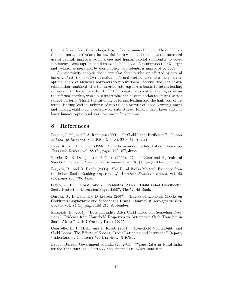
We show that this regulation has led to strong rationing on the small loanmarket. Indeed, the survey data of rural households we use show that 82%of loans are below Rs 25,000 (US$500) and only 1.5% are above the thresholdof Rs 200,000.2 In addition, we find no evidence of banks applying differentconditions for different risk types, despite empirical evidence that it is possibleto discriminate. To study the consequences of this rationing on the agrarianeconomy in rural India, we build an overlapping-generations model with formaland informal lending where farms have different risk characteristics and are loan-rationed. Households supply labor, possibly including child labor, competitivelyand accumulate human capital.
Others have documented that small rural farms in India are subject to loanrationing they cannot overcome with equity. Burgess and Pande (2005) docu-ment that forcing banks to open branches in rural India reduced poverty andincreased wages and education. Sometimes the lack of equity is overcome withchild labor. For example, Singh (2011) shows that adverse economic shocksleads to lower school enrollment in India. Similar effects have been found inSouth Africa (Edmonds 2004), Tanzania (Beegle, Dehejia, and Gatti 2006), andBrazil (Duryea, Lam, and Levison 2007).
After calibrating the model economy to current macroeconomic conditionsand outcomes of the survey data (which include 22% of a child’s time devotedto labor), we study the consequences of removing the interest rate regulationand allowing the banks to discriminate across risk types. The results of marketpricing are dramatic: Informal lending and child labor both disappear and thewelfare of every household improves on average by a consumption equivalent of
1After the initiation of financial sector reforms in the early 1990s, the Reserve Bank ofIndia (RBI) took various steps to deregulate the lending rates of commercial banks. Theslabs or credit limit size class under the RBI’s revised guidelines of 1993 consisted of threecategories: (i) advances up to and inclusive of Rs 25,000; (ii) advances over Rs 25,000 andup to Rs 200,000; and (iii) advances over Rs 200,000. In a major step toward deregulation oflending rates, the RBI decided in October 1994 that banks would determine their own lendingrates for credit limits over Rs 200,000. This decision was reached in accordance with banks’risk-reward perception and commercial judgment. At the same time, banks were required todeclare their prime lending rate (P1). In 1998, the P1 was converted as a ceiling rate on loansup to Rs 200,000. The rationale for this policy was that the P1, as the rate chargeable to thebest borrower of the bank, should be the maximum rate chargeable to the small borrowers.This system continued until 2009-10 when the Base Rate system replaced it, taking effect onJuly 1, 2010. The Base Rate is currently the minimum rate for all loans and serves as a ceilingfor small loans up to Rs 200,000 (Reserve Bank of India, 2009, 2010).
2See Table 1 for details.
2
almost 60%.The rationing regime is characterized by high capital costs, since rural infor-
mal moneylenders charge much more than the formal banking sector, underaccu-mulation of physical capital, and low wages. This situation forces parents tosend their children to work to meet subsistence consumption. The resultingunder-accumulation of human capital exacerbates the low wages and reinforceschild labor. This vicious cycle is broken by deregulation of lending, allowing thesubstitution of labor for capital, both physical and human.
Are parents selfish if they send their children to work? Significant researchtakes this a starting point—for example, in Basu and Van (1998); Baland andRobinson (2000); Ranjan (2001); Cigno, Rosati, and Tzannatos (2002); andGuarcello, Mialli, and Rosati (2003). The premise is that developing economiestypically have a comparative advantage in unskilled labor-intensive goods. Un-der such circumstances, sending a child to school would not be the optimalchoice of a household head, who could increase family income and possibly hisown leisure by sending children to work. We argue that with more capital avail-able for production, such an outcome may be avoidable and this capital canbe obtained by deregulating small loans. Also, Ray (2002) shows that creditconstraints can force a household to use child labor to satisfy subsistence con-sumption. In our case, we show that credit markets regulated in a particularway can induce child labor even with altruistic parents, also because of subsis-tence consumption. In addition, deregulation has a macroeconomic impact byincreasing wages and thus making education more valuable.
Other financial market inefficiencies may trigger child labor. Baland andRobinson (2000) and Rajan (1999) show that because parents cannot borrowagainst their children’s future income, they do not fully internalize the valueof education. Pallage and Zimmermann (2007) show how direct transfers can(slowly) eradicate child labor.
The study is organized as follows. Section 2 discusses the model economy,which is then differentiated in Section 3 for the banking sectors between theregulated, nondiscrimating regime that leads to loan rationing and the deregu-lated, discriminating regime. To obtain quantitative answers, we then calibratethe economy using a survey of rural loan applicants in Section 4. We then dis-cuss results in Section 5, including a sensitivity analysis in Section 6. The lastsection concludes.
2 The Baseline Model
In this section, we describe a three-period overlapping-generations model withfour types of agents: households, farms, banks, and moneylenders. Householdshave one unit of time to devote to human capital accumulation or child laborin the first period. In the second period, labor income, including income fromchildren, is split between present consumption and savings for the third period,retirement.
Farms are heterogeneous with respect to the riskiness of their unique projects.
3
They use labor only for production and need to borrow to pay for wages. Ifa farm’s loan is rejected by a bank, it turns to the informal market for a loanfrom moneylenders.
We consider two banking regimes: In the first, credit rationing is prevalentas banks are tied to a government-mandated loan rate applicable to all loans.In the second, banks are free to set interest rates and discriminate.
Finally, moneylenders set interest rates freely given their cost structure. Wenow describe the components of the model in detail.
2.1 Households
Each member of a household lives for three periods. In the first (t− 1), a childcan use his time allotment for education (et−1) or work (1 − et−1), but this isa decision made by parents. If working, a child earns at the wage rate of wC
t−1,which goes to the parents. Children do not consume.
In the second period, t, the child becomes an adult and uses the entire timeendowment for work, paid at the efficiency rate wA
t . Efficiency depends on thelevel of human capital ht. The total income of the adult (from his own work
and his child’s work) is distributed between immediate consumption (ct,At ) and
deposits at the bank (Dt).Deposits mature in the third period (t + 1), and the old agent consumes
deposits plus interest (ct,Ot+1 = (1+rd,t)Dt). Agents care about their consumption
in the second and third period, taking into account minimum subsistence c, andthey are concerned about their child through her human capital. Thus theproblem of the household is
Vt(ht) = maxet,ht+1,ct
ln
(
ct,At +
ct+1,Ot+1
1 + rdt
− c
)
+ σVt+1(ht+1),
S. T. ct,At + Dt ≤ wA
t ht + wCt (1 − et),
ct,Ot+1 ≤ (1 + rd
t )Dt,
where σ is an altruism parameter. We follow Pallage and Zimmermann (2007)and define the human capital accumulation as follows:
ht+1 = ξ1eξ2
t hξ3
t ,
where 0 < ξ2, ξ3 < 1 and h > 1. Define ω as the ratio of the child wage to the
adult wage, ω =wC
t
wAt
. Clearly, with wA and wC as the efficiency wage, the value
of ω will depend on the respective human capitals of the adult and children ofthe households. Then we can obtain from the first-order conditions the supplyof child labor,
nCt = max
0, 1 −
(
σξ1ξ2hξ3
t wAt+1
ωwAt
)1
1−ξ2
.
4
Thus, if the adult wage and human capital are high enough, it is possible to haveno child labor in the steady state as long as the various parameter values satisfyσξ1ξ2hξ3
ω> 0. As all parameters are positive, this is the necessary condition in
our model economy to reach an equilibrium that theoretically is child labor free.
2.2 Farms
We consider agricultural farms in rural India as the major production unit inour model economy. There are two types of farms, high-risk and low-risk, andthe type is private information. They are otherwise identical; in particular,they have the same output when they succeed (or fail). High-risk farms preferto borrow less because of their higher chances of failure. Low-risk farms, on theother hand, have a lower chance of failure and hence, have higher demand forloans. They need loans to finance their only input: labor. They can use twotypes of labor, adult and child, that are perfectly substitutable, although theefficiency of child labor is ω
htthat of adult labor.3 Let the production function
be
f(ht, nCt ) = A
(
ω(ht)nCt
)m.
Define γi as the probability of success of a firm depending on its risk; i = 0for high-risk farms, and 1 for low-risk farms. The term lt is the interest ratepaid on loans. Then the expected profits are
γiA(
ω(ht)nCt
)m− (1 − lt)
(
ω(ht)nCt
)
.
The farm maximizes these expected profits by choosing the appropriate levelof child labor, as adult labor is a given. Thus, the demands for child labor andfor loans are
nCt = max
{
0,
(
ωiAm
(1 + lt)wAt
)1
1−m
− ht
}
,
LiDt =
(
ωiAm
(1 + lt)(wAt )m
)1
1−m
.
2.3 Banks
Banks are the suppliers of loans in the formal market. They take loan applica-tions and decide how many loans to provide and, depending on the environment,what interest rate to charge. Here, we look at two different regimes for the creditmarket. In the first, there is credit rationing because the interest rate is set by
3One could also assume that the success rate could depend on the use of child labor. Thiswould make an analytical solution impossible but would only reinforce our results. Indeed, aswe show later, changes in the success rate have an impact, but the presence of credit rationingis of first-order importance. Thus, we have neglected this feature in the model for tractability.
5
the government at a low level, and banks are not allowed to price discriminate.In the second, the government lifts all restrictions and thus allows banks todifferentiate the interest rate by firm characteristics—in our case, riskiness—without bounds on the interest rate.
2.3.1 Credit Rationing Regime
Banks have no control over the interest rate for loans, l̄, and cannot use in-formation to discriminate across lenders. In our case (India), this is mandatedby government policy: banks must lend at a regulated interest rate, and theycannot offer conditions that differ across lenders. This encourages more high-risk farms to apply for loans. Banks are then forced to adopt indiscriminatecredit rationing as a hedging device against default risks. Under this regime,banks supply only a fraction of the market with loans even if they have suffcientresources to meet the total demand.
Thus, banks can supply only a fraction α of loans demanded, a fraction thatis endogenously determined based on the administered loan rate and the successrate of the farms. Since banks cannot discriminate, low-risk farms with highdemand will take the guise of high-risk farms with low demand. This adverseselection problem in the formal loan market leads the high-demand farms to reapsome surplus by operating on the lower demand curve. Let ρ be the proportionof high-risk farms; then the total demand for loans is
LDt = ρ
(
ω0Am
(1 + l̄)(wAt )m
)1
1−m
+ (1 − ρ)
(
ω1Am
(1 + l̄)(wAt )m
)1
1−m
. (1)
However, the total demand revealed on the formal market is
LFDt =
(
ω0Am
(1 + l̄)(wAt )m
)1
1−m
,
as low-risk farms masquerade as high-risk ones. Finally, the total supply ofloans of the formal loan market is
LFSt = α
(
ω0Am
(1 + l̄)(wAt )m
)1
1−m
. (2)
Banks maximize profits by choosing how much to ration the demand:
maxα
αφ0 l̄LFDt − rd
t Dt,
S. T. αLFDt ≥ Dt.
The optimal choice is then
α∗ =rdt
l̄φ0. (3)
Note that α∗ is inversely related to the success rate of high-risk farms. Thispoint is important in our analysis.
6
2.3.2 Self-Revelation Regime
Under this regime, banks are free to set the loan rate, in particular to discrimi-nate among applicants. Different loans are offered at different rates, and farmsself-select following the direct revelation principle of Myerson (1979).
The self-revelation of the farms operates through their demand coefficients,which depends on their risk level. High-risk farms have a lower demand coeffi-cient γ0 and banks try to set the loan rate so they can obtain all the surplus.Thus, given the probability of success φ0, the participation constraint is binding,
Et(R0t ) = φ0L
0t (l
0t ),
where R0t is banks’ revenue from high risk farms.
Low-risk farms have a higher demand coefficient, γ1, because of their highersuccess rate but have the incentive to operate on the lower demand curve of thehigh-risk farms. Thus, they should be bound by the incentive constraint. Todetermine this, first note that the surplus enjoyed by low-risks farms when theymasquerade as high-risk farms is
Am
(
L0t
wAt
)m
(γ1 − γ0). (4)
This surplus is constructed in the following manner: for low-demand farms(high- and low-risk farms separately), the willingness to pay under the twocontracts is defined by
1 + l0t =γ0Am
(wAt )m(L0
t )1−m
, (5)
1 + l1t =γ1Am
(wAt )m(L0
t )1−m
. (6)
Thus, for the same size loan a low-risk farm has a willingness to pay γ1−γ0
(wAt )m(L0
t)1−m
higher, and its surplus is
γ1 − γ0
(wAt )m(L0
t )1−m
L0t ,
which is the same as the surplus shown above in Equation 4. Therefore, theincentive constraint for the low-risk farm needs to be
Et(R1t ) = φ1L
1t (l
1Tt) − Am
(
L0t
wAt
)m
(γ1 − γ0),
where R1t is the banks’ revenue from low-risk farms and Tt is the demand for in-
formal loans (to be determined shortly below). Then, the maximization problemof the banks with ρ as the proportion of high-risk farms, is
7
maxL0
t ,L1t
ρEt(R0t ) + (1 − ρ)Et(R
1t ) − rd
t Dt,
S. T. Et(R1t ) = φ1L
1t (l
1Tt) − Am
(
L0t
wAt
)m
(γ1 − γ0),
Et(R0t ) = φ0L
0t (l
0t ),
Dt = ρL0t + (1 − ρ)L1
t .
It follows that the optimal loan rates are
l0t =rdt
φ0+
1 − ρ
ρφ0
Am2(γ1 − γ0)
(wAt )m(L0
t )1−m
, (7)
l1t =rdt
φ1. (8)
2.4 Moneylenders
moneylenders operate on the informal loan market and try to satisfy any demandfor loans that has not been satisfied on the formal market. Their operation costsare higher than those of banks; thus, moneylenders are active only in the creditrationing regime. The demand for loans they face is the revealed demand thatwas rationed, LD
t − LFSt , and the demand that low-risk farms were hiding to
masquerade as high-risk farms. The demand for informal loans that spills overfrom the formal market is thus
Tt = (1−α)
(
γ0Am
(1 + l̄)(wAt )m
)1
1−m
+(1−ρ)
(
Am
(1 + l̄)(wAt )m
)1
1−m(
γ1
1−m
1 − γ1
1−m
0
)
.
Now suppose that η is the proportion of high-risk farms in the informaldemand mix. Then the demand from the two risk types that moneylenders facecan be defined as
M0t = η(1 − α)
(
γ0Am
(1 + l̄)(wAt )m
)1
1−m
, (9)
M1t =
(
Am
(wAt )m(1 + l̄)
)1
1−m(
(ρ + ηα − η − α) γ1
1−m
0 + (1 − ρ) γ1
1−m
1
)
.(10)
We assume that the informal moneylenders have the ability to discriminatebetween the types of loan seekers, as they are not constrained by governmentoversight. They can set loan rates differently for high- and low-risk farms. Theymaximize the following profits:
maxM0
t ,M1t
EtΠt = φ0lh,0t M0
t + φ0lh,1t M1
t − (c0M0t + c1M1
t ), (11)
8
where ci is a cost coefficient for raising funds and monitoring loans, and φi isthe success rate of firm with type i. From the first-order conditions, we canthen infer the loan rates moneylenders charge:
lh,0t =
c0
(1 − α)ηφ0, (12)
lh,1t =
c1
(1 − η)(1 − α)φ1. (13)
3 The Two Regimes
We now evaluate the steady-state equilibrium of the model economy. As thereare two different regulatory environments in the formal banking sector, we needto analyze them separately. We first turn to the current situation in India, witha cap on loan rates and no loan discrimination.
3.1 Credit Rationing
From the total supply of formal loans (Equation 2) and equilibrium rationingby formal banks (Equation 3), we obtain formal loans as a function of wages,
LFt =
rdt
l̄φ0
(
γ0Am
wAt (1 + l̄)
)
.
From the demand for informal loans from high-risk farms (Equation 9), theequilibrium rationing by formal banks (Equation 3), and the loan rate choiceof moneylenders (Equation 12), we get informal loans of high-risk farms as afunction of wages,
M0t = η
(
1 −rdt
l̄φ0
)
(
γ0Am
wAt (1 + c0
(1−α)ηφ0 )
)
.
Similarly for low-risk farms (Equations 3, 10, and 13), we determine theinformal loans to low-risk farms,
M1t =
(
(
γ0)
11−m
(
ρ +ηrd
t
l̄φ0− η −
rdt
l̄φ0
)
+ (1 − ρ)(
γ1)
11−m
)
.
Equating the sum of the three equations above to the demand for loans(Equation 1), we obtain the equilibrium adult wage, wA
t , an equation too longto report here. Since the wages of adults and children are equal to their re-spective marginal products, farms are indifferent to either type of labor. It istherefore entirely up to the household to supply child labor or not. As parentsare altruistic (they like to have their children educated), child labor is suppliedonly when minimum consumption cannot be covered with adult income. Thus,
9
nC = 0 if wAt ht > c,
= 1 −
(
σξ1ξ2hξ3t
ω(ht)
)1
1−ξ2
otherwise,
where ω(ht) is the ratio of the child wage to the adult wage and depends on therespective human capital. There is no child labor if
ω(ht) ≤ σξ1ξ2hξ3
t (14)
wAt ≥
c
ht
.
3.2 Self-Revelation
Since banks can discriminate, they can serve the entire market and moneylendershave no role. By equating the high-risk farms’ willingness to pay to the banks’willingness to accept (Equations 5 and 7), and correspondingly for low risk loans(Equations 6 and 8), we obtain the equilibrium quantity of high- and low-riskloans,
LSR0 =
(
Am(γ0ρφ0 − m(1 − ρ)(γ1 − γ0))
(wA)mρ(φ0 + rd,ss)
)1
1−m
,
LSR1 =
(
Amφ1γ1
(wA)m(φ1 + rd,ss)
)1
1−m
,
which add up to a total loan supply of LSR = ρLSR0 +(1− ρ)LSR
1 . We can thenobtain the two steady-state lending rates,
l0,ss =γ0ρrd,ss + m(1 − ρ)(γ1 − γ0)
γ0ρφ0 − m(1 − ρ)(γ1 − γ0),
l1,ss =rd,ss
φ1.
Notice that the low-risk loan is inversly dependent on farms’ success rate, andthe higher the success rate the lower is the low-risk loan rate. The high-risk loanrate, however, has a premium attached to it (the component m(1−ρ)(γ1−γ0)),which is mostly decided by the gap, γ1−γ0). This suggests that when a farm typeis known, banks can easily assign a differentiated price by rewarding the low-riskfarms with a lower loan rate. Finally, we determine the adult equilibrium wagethat satisfies the necessary condition of no child labor as follows:
10
wA =1
h1−m
[
ρ
(
Am(γ0ρφ0 − m(1 − ρ)(γ1 − γ0))
ρ(φ0 + rd,ss)
)1
1−m
+(1 − ρ)
(
Amφ1γ1
φ1 + rd,ss
)1
1−m
]1−m
.
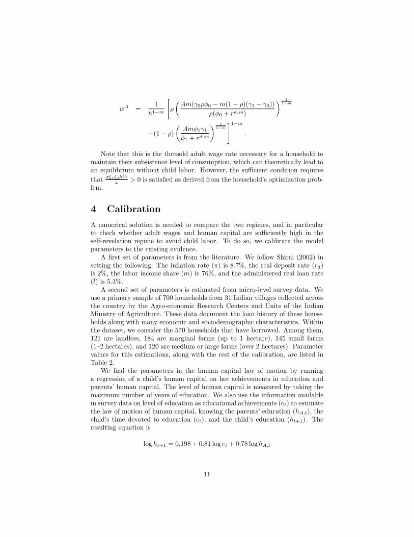
Note that this is the thresold adult wage rate necessary for a household tomaintain their subsistence level of consumption, which can theoretically lead toan equilibrium without child labor. However, the sufficient condition requires
that σξ1ξ2hξ3
ω> 0 is satisfied as derived from the household’s optimization prob-
lem.
4 Calibration
A numerical solution is needed to compare the two regimes, and in particularto check whether adult wages and human capital are sufficiently high in theself-revelation regime to avoid child labor. To do so, we calibrate the modelparameters to the existing evidence.
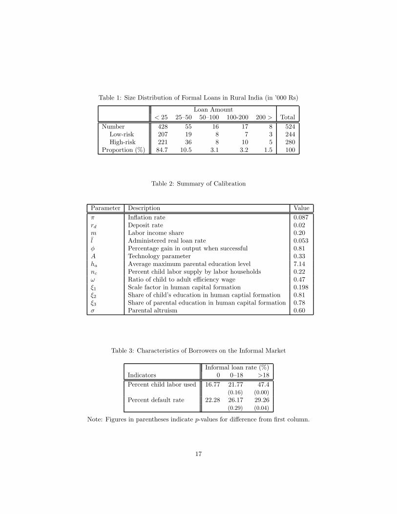
A first set of parameters is from the literature. We follow Shirai (2002) insetting the following: The inflation rate (π) is 8.7%, the real deposit rate (rd)is 2%, the labor income share (m) is 76%, and the administered real loan rate(l̄) is 5.3%.
A second set of parameters is estimated from micro-level survey data. Weuse a primary sample of 700 households from 31 Indian villages collected acrossthe country by the Agro-economic Research Centers and Units of the IndianMinistry of Agriculture. These data document the loan history of these house-holds along with many economic and sociodemographic characteristics. Withinthe dataset, we consider the 570 households that have borrowed. Among them,121 are landless, 184 are marginal farms (up to 1 hectare), 145 small farms(1–2 hectares), and 120 are medium or large farms (over 2 hectares). Parametervalues for this estimations, along with the rest of the calibration, are listed inTable 2.
We find the parameters in the human capital law of motion by runninga regression of a child’s human capital on her achievements in education andparents’ human capital. The level of human capital is measured by taking themaximum number of years of education. We also use the information availablein survey data on level of education as educational achievements (et) to estimatethe law of motion of human capital, knowing the parents’ education (hA,t), thechild’s time devoted to education (et), and the child’s education (ht+1). Theresulting equation is
log ht+1 = 0.198 + 0.81 log et + 0.78 loghA,t
11
The parental altruism parameter (σ) is obtained by substituting the aboveregression parameters into Equation 14. The supply of child labor nc is obtainedby determining the average time spent working from the data sample, which is22%.
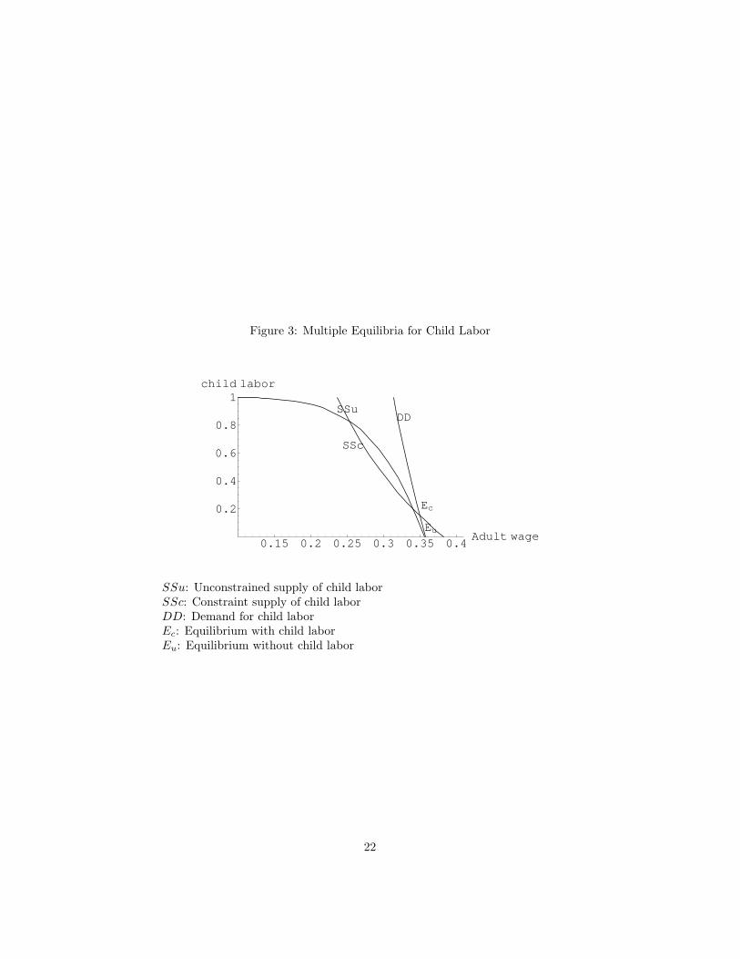
An analysis of the loan rates in the dataset reveals a clear separating equi-librium in the informal market, reflecting the fact that moneylenders are ableto discriminate between high and low risks. Figure 1 shows separations at loanrates of 3% and 18% and modes at 0%, 15% and 27%. Clearly, a zero interestrate is not consistent with our model of moneylenders and must have some otherorigin (loans from relatives or loans with nonmonetary interest). We thus onlyconsider the separation at 18%.4
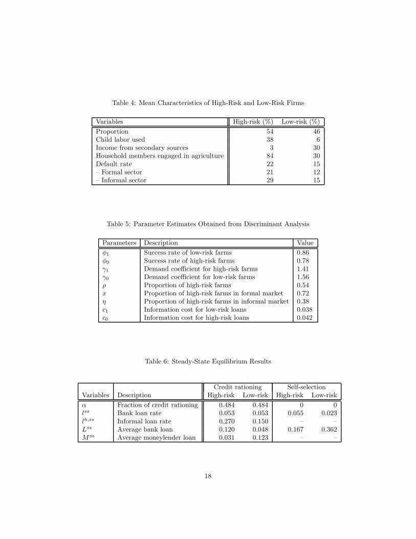
Now that we have separated these borrowers into two groups, we use discrim-inant analysis to determine the characteristics of high- and low-risk borrowers.In particular, we verify that high risk ones have higher default rates, have lowerdiversification in their sources of income, and use more child labor (as a meansto absorb shocks). Table 3 shows that the first and last are verified across thethree interest rate modes. Table 4 verifies all hypotheses after classifying bor-rowers by risk. It is particularly interesting to see how well the characteristicsof high and low risk borrowers are distinguishable and that the formal marketsis clearly missing opportunities to discriminate.
From this discriminant analysis we can establish the value of a series ofparameters (Table 5). The proportion of high-risk borrowers (ρ) is 54%; theseborrowers have a success rate (φ0) of 78%, compared with an 86% success ratefor low-risk ones (φ1). From this one can infer the demand coefficients for both(γ1 and γ0) at 1.41 and 1.56, respectively. Finally, we find the proportion ofhigh-risk farms in the informal loan market to be 38% and 72% in the formalmarket. Using equilibrium conditions of the model—Equations 9, 10, 12, and13—and the moneylender interest rates, one can then find the information costcoefficients c1 and c0, which are 0.038 and 0.042,respectively.
The last parameter is estimated from a different source. The ratio of the childto the adult efficient wage (ω) is from the Labour Bureau of the Governmentof India (2002–2003), which publishes monthly average wages for men, women,and child laborers. We convert the adult wage to an efficient wage by dividingby years of education as a proxy for human capital. For children, we assumethey are all at the same efficiency, unless they finish elementary schooling. Weobtain a ratio of 47%.
5 Outcomes
Now that we have determined values for all parameters in the model, wherewe assumed that rationing was taking place as is currently the case in India,we establish some further characteristics of this regime. Subsequently, we allow
4Various estimates show that zero-interest borrowers have the same characteristics as low-risk borrowers; therefore, we combine them.
12
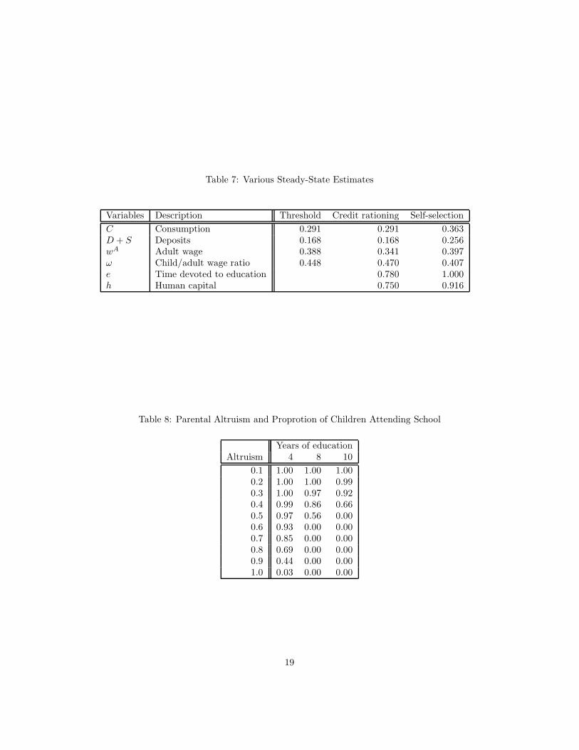
formal banks to discriminate and set loan rates to observe how the equilibriumdiffers (Tables 6 and 7). But we first look at the rationing regime.
With the loan rate ceiling, our findings from the survey data show that 48.4%of borrowers are rejected by the formal credit sector. If they obtain a loan,high-risk borrowers manage to get a larger loan than low-risk ones. One reasoncould be that because of lower demand from high-risk farms, they might havebeen treated as small borrowers and hence were served better. Borrowers whouse the informal sector pay much higher interest rates—22% more for high-riskborrowers and 10% more for low-risk ones—and the latter receive larger loans.Essentially, we see that moneylenders exercise the discrimination that formalbanks cannot, but at a much higher price.
As a consequence, loans are rare and expensive, leading to a stronger re-liance on the labor input, particularly on child labor, as children spend 22% oftheir time working. Obviously, steady-state human capital is then low, leadingto low adult wages, which reinforces the need for child labor, and finally lowconsumption.
Note that there may be a second equilibrium in a regulated loan market,an equilibrium without child labor. We do not consider it here because themodel is calibrated to the Indian economy, which exhibits child labor. Figure 3shows that if the adult wage is high enough, an outcome without child labor ispossible. It is, however, much easier to reach higher wages when more capitalis available.
Now let us turn to the liberalized regime where formal banks can choosethe interest rate and discriminate across borrower risk categories. Evidently,this scenario crowds out the moneylenders, since every borrower is now served.Formal loan rates are slightly higher for high risks, but massively lower for lowrisks compared with credit rationing. Both types obtain much larger loans,especially low risks.
The consequence is that every child can now attend school full-time. Thisis a consequence of several effects: First, the much higher loan mass inducesa higher use of capital. Second, adult wages are now higher, and above thesubsistence level (thanks to higher physical and human capital) and sufficientto allow households to rely only on adult incomes. This occurs despite the factthat in absolute terms child wages have increased but have decreased in relativeterms. Finally, we observe that consumption is now 25% higher. Even better,as their child’s welfare is now higher, the utility of the parents is now raised inconsumption equivalence terms by 59% (Table 7).
6 Sensitivity Analysis
In this section, we seek to understand the sensitivity of our results to vari-ous changes in the parametrization, particularly those parameters that have animpact on child labor.
Figure 2 documents, for a given level of parental education, (7.14 years ofeducation, taken from the empirical average) the child labor supply as it varies
13
according to the parents’ altruism, σ. We note that the unconstrained supply ofchild labor (SSu) decreases monotically with altruism, which is expected, but itdrops faster around 0.60, our calibration value of σ. It would thus appear thatchild labor should be easy to eradicate. However, this schedule changes markedlyif one takes into account that child labor is used when needed to sustain mini-mum consumption (SSc). Clearly, a necessary condition for the eradication ofchild labor is to obtain subsistence consumption without requiring the help ofchildren. Even with high levels of altruism, subsistence consumption remains abottleneck. As our results indicate, an easy way to remove this bottleneck is toimprove the earning capacity of the adults, which can be obtained by increasingproductive capital through loans, and this can be achieved by liberalizing thecredit market.
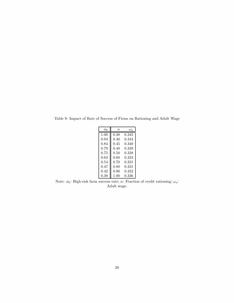
Allowing both parental education and altruism to vary reveals more inter-esting insights. Table 8 shows that both are important to eradicate child labor.While altruism is a given, the parents’ education is endogenous in the long runand can be increased, as seen in our benchmark experiment, by increasing wages,which itself can be be obtained by removing credit rationing. This means thateducation can be a powerful substitute for altruism.
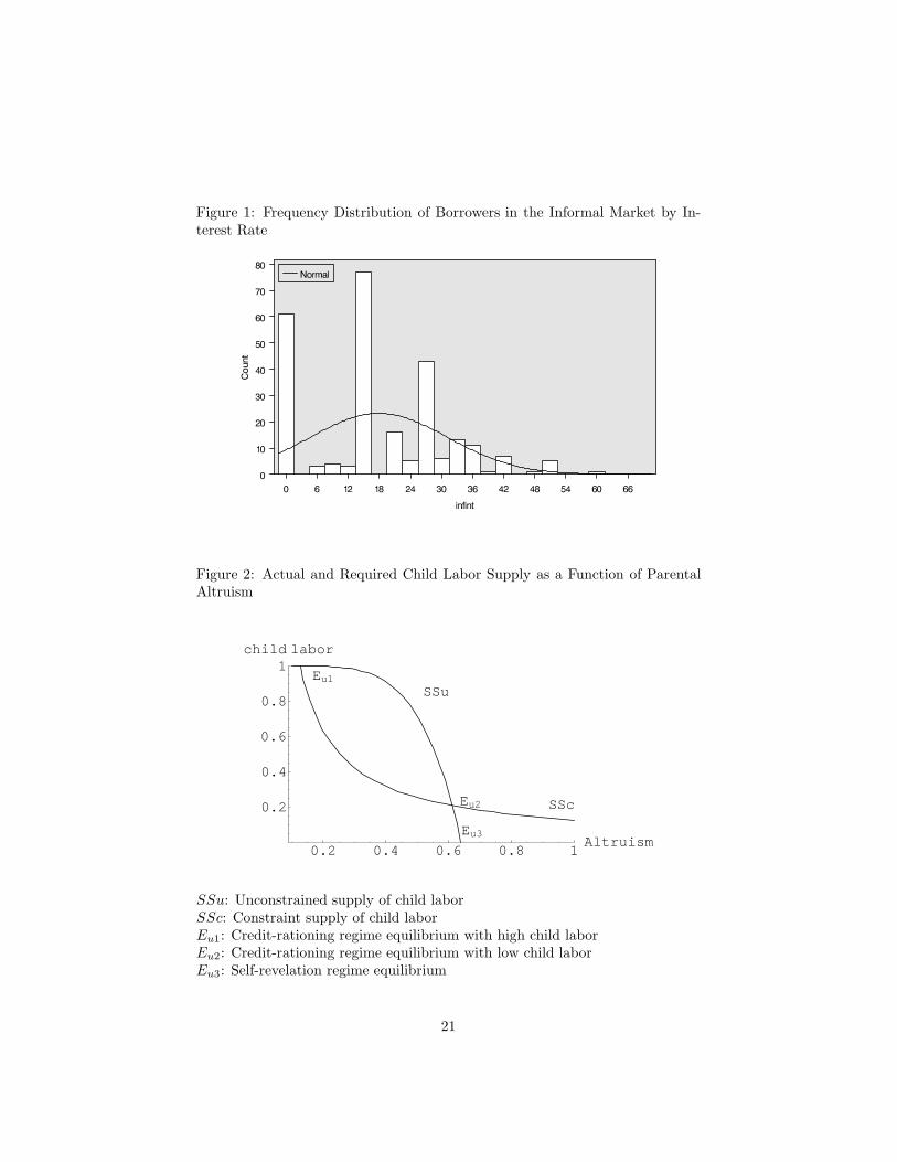
Credit rationing can also have some rather perverse implications. Supposewe improve the success rate of high-risk farms. On first sight, this should havepositive implications for the economy. But when there is no discrimination inlending, this increases the demand for loans. Since there is an interest rateceiling, this makes rationing more severe. As high-risk farms increase their loanshare, the resulting capital and adult wages both decrease, making child laborworse (Table 9). Increasing the success rate of low-risk farms also has adverseconsequences under credit rationing, through adverse selection: As farms hidetheir extra demand, it spills over to the informal market, increasing farms’ costsand their dependence on informal lending sources.
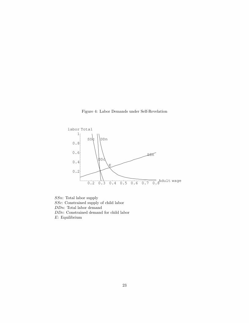
Figure 4 for the self-revelation regime shows that both the demand for childlabor (DDc) and the supply of child labor (SSc) are inelastic, with supply havinga less steep slope. At the threshold adult wage (3.88), the supply of child laborreaches a corner solution with a zero child labor supply. We find that under theself-revelation regime, the adult wage rate is higher (3.97) than this thresoldrate, which leads the adult labor market to clear, and the child labor marketbecomes suboptimal with an interior solution.
7 Conclusion
India imposes caps on lending rates in rural areas and forbids lenders fromdiscriminating across small borrowers. We study the impact of this regulationon household outcomes, particularly the use of capital and child labor. Todo so, we first build a model economy that replicates outcomes from a surveyof Indian households, in particular with respect to lending rates, the use ofinformal moneylenders, and child labor. Then we remove the lending regulationand find that the formal sector can then fully serve the loan demand at rates
14
that are lower than those charged by informal moneylenders. This increasesthe loan mass, particularly for low-risk borrowers, and thanks to the increaseduse of capital, improves adult wages and human capital sufficiently to coversubsistence consumption and thus avoid child labor. Consumption is 25% largerand welfare, as measured by consumption equivalents, is improved by 59%.
Our sensitivity analysis documents that these results are affected by severalfactors. First, the nondiscrimination of formal lending leads to a higher-than-optimal share of high-risk borrowers to receive loans. Second, the lack of dis-crimination combined with the interest rate cap forces banks to ration lendingconsiderably. Households then fulfill their capital needs at a very high cost onthe informal market, which also undertakes the discrimination the formal sectorcannot perform. Third, the rationing of formal lending and the high cost of in-formal lending lead to underuse of capital and overuse of labor, lowering wagesand making child labor necessary for subsistence. Finally, child labor sustainslower human capital and thus low wages for everyone.
8 References
Baland, J.-M., and J. A. Robinson (2000). “Is Child Labor Inefficient?” Journal
of Political Economy, vol. 108 (4), pages 663–679, August.
Basu, K., and P. H. Van (1998). “The Economics of Child Labor,” American
Beegle, K., R. Dehejia, and R Gatti (2006). “Child Labor and AgriculturalShocks,” Journal of Development Economics, vol. 81 (1), pages 80–96, October.
Burgess, R., and R. Pande (2005). “Do Rural Banks Matter? Evidence fromthe Indian Social Banking Experiment,” American Economic Review, vol. 95(3), pages 780–795, June.
Cigno, A., F. C. Rosati, and Z. Tzannatos (2002). “Child Labor Handbook,”Social Protection Discussion Paper 25507, The World Bank.
Duryea, S., D. Lam, and D Levison (2007). “Effects of Economic Shocks onChildren’s Employment and Schooling in Brazil,” Journal of Development Eco-
nomics, vol. 84 (1), pages 188–214, September.
Edmonds, E. (2004). “Does Illiquidity Alter Child Labor and Schooling Deci-sions? Evidence from Household Responses to Anticipated Cash Transfers inSouth Africa,” NBER Working Paper 10265.
Guarcello, L., F. Mialli, and F. Rosati (2003). “Household Vulnerability andChild Labor: The Effects of Shocks, Credit Rationing and Insurance,” Report,Understanding Children’s Work project, UNICEF.
Labour Bureau, Government of India (2002–03). “Wage Rates in Rural Indiafor the Year 2002–2003,” http://labourbureau.nic.in/wrr2sum.htm
15
Myerson, R. (1979). “Incentive Compatibility and the Bargaining Problem,”Econometrica, vol. 47 (1), pages 61–73, January.
Nardinelli, C. (1990). Child Labor and the Industrial Revolution, Indiana Uni-versity Press, Bloomington.
Pallage, P., and C. Zimmermann (2007). “Buying Out Child Labor,” Journal
of Macroeconomics, vol. 29 (1), pages 75–94, March.
Ranjan, P. (2001). “Credit Constraints and the Phenomenon of Child Labor,”Journal of Development Economics, vol. 64 (1), pages 81–102, February.
Ray, R. (2002). “Simultaneous Analysis of Child Labor and Child School-ing: Comparative Evidence from Nepal and Pakistan,” Economics and Political
Weekly, pages 5215–5224, December 28.
Reserve Bank of India (2009). “Report of the Working Group on BenchmarkPrime Lending Rate,” October 2009.
Reserve Bank of India (2010). “Regulation and Supervision of Financial Insti-tutions,” Annual Report 2009–2010, Chapter VI, August 2010.
Shirai, S. (2002). “Road from State to Market: Assessing the General Approachto Banking Sector Reform in India,” Research Paper 32, Asian DevelopmentBank Institute.
Singh, K. (2011). “Impact of Adverse Economic Shocks on the Indian ChildLabour Market and the Schooling of Children of Poor Households,” MPRAPaper 30958, University Library of Munich, Germany.
16
Table 1: Size Distribution of Formal Loans in Rural India (in ’000 Rs)
π Inflation rate 0.087rd Deposit rate 0.02m Labor income share 0.20l̄ Administered real loan rate 0.053φ Percentage gain in output when successful 0.81A Technology parameter 0.33ha Average maximum parental education level 7.14nc Percent child labor supply by labor households 0.22ω Ratio of child to adult efficiency wage 0.47ξ1 Scale factor in human capital formation 0.198ξ2 Share of child’s education in human captial formation 0.81ξ3 Share of parental education in human capital formation 0.78σ Parental altruism 0.60
Table 3: Characteristics of Borrowers on the Informal Market
Informal loan rate (%)Indicators 0 0–18 >18
Percent child labor used 16.77 21.77 47.4(0.16) (0.00)
Note: Figures in parentheses indicate p-values for difference from first column.
17
Table 4: Mean Characteristics of High-Risk and Low-Risk Firms
Variables High-risk (%) Low-risk (%)
Proportion 54 46Child labor used 38 6Income from secondary sources 3 30Household members engaged in agriculture 84 30Default rate 22 15– Formal sector 21 12– Informal sector 29 15
Table 5: Parameter Estimates Obtained from Discriminant Analysis
Parameters Description Value
φ1 Success rate of low-risk farms 0.86φ0 Success rate of high-risk farms 0.78γ1 Demand coefficient for high-risk farms 1.41γ0 Demand coefficient for low-risk farms 1.56ρ Proportion of high-risk farms 0.54x Proportion of high-risk farms in formal market 0.72η Proportion of high-risk farms in informal market 0.38c1 Information cost for low-risk loans 0.038c0 Information cost for high-risk loans 0.042
C Consumption 0.291 0.291 0.363D + S Deposits 0.168 0.168 0.256wA Adult wage 0.388 0.341 0.397ω Child/adult wage ratio 0.448 0.470 0.407e Time devoted to education 0.780 1.000h Human capital 0.750 0.916
Table 8: Parental Altruism and Proprotion of Children Attending School
Figure 1: Frequency Distribution of Borrowers in the Informal Market by In-terest Rate
Figure 2: Actual and Required Child Labor Supply as a Function of ParentalAltruism
0.2 0.4 0.6 0.8 1Altruism
0.2
0.4
0.6
0.8
1child labor
SSu
SSc
Eu1
Eu2
Eu3
SSu: Unconstrained supply of child laborSSc: Constraint supply of child laborEu1: Credit-rationing regime equilibrium with high child laborEu2: Credit-rationing regime equilibrium with low child laborEu3: Self-revelation regime equilibrium
21
Figure 3: Multiple Equilibria for Child Labor
0.15 0.2 0.25 0.3 0.35 0.4Adult wage
0.2
0.4
0.6
0.8
1child labor
SSu
SSc
DD
Ec
Eu
SSu: Unconstrained supply of child laborSSc: Constraint supply of child laborDD: Demand for child laborEc: Equilibrium with child laborEu: Equilibrium without child labor
22
Figure 4: Labor Demands under Self-Revelation
0.2 0.3 0.4 0.5 0.6 0.7 0.8Adult wage
0.2
0.4
0.6
0.8
1labor Total
DDnSSc
DDcSSn
E
SSn: Total labor supplySSc: Constrained supply of child laborDDn: Total labor demandDDc: Constrained demand for child laborE: Equilibrium