Local and Nonlocal Discrete Regularization on Weighted

Graphs for Image and Mesh Processing

Sebastien Bougleux (sebastien.bougleux@greyc.ensicaen.fr)ENSICAEN - GREYC CNRS UMR 6072 - Equipe Image6 BD du Marechal Juin, 14050 Caen Cedex France

Abderrahim Elmoataz (abder@greyc.ensicaen.fr)Universite de Caen - GREYC CNRS UMR 6072 - Equipe ImageBD du Marechal Juin, 14050 Caen Cedex France

Mahmoud Melkemi (mahmoud.melkemi@uha.fr)Univertsite de Haute-Alsace - LMIA - Equipe MAGE4 rue des Freres Lumiere, 68093 Mulhouse Cedex France

Abstract. We propose a discrete regularization framework on weighted graphs of arbitrarytopology, which unifies local and nonlocal processing of images, meshes, and more generallydiscrete data. The approach considers the problem as a variational one, which consists inminimizing a weighted sum of two energy terms: a regularization one that uses the discrete p-Dirichlet form, and an approximation one. The proposed model is parametrized by the degree pof regularity, by the graph structure and by the weight function. The minimization solutionleads to a family of simple linear and nonlinear processing methods. In particular, this familyincludes the exact expression or the discrete version of several neighborhood filters, such as thebilateral and the nonlocal means filter. In the context of images, local and nonlocal regulariza-tions, based on the total variation models, are the continuous analogue of the proposed model.Indirectly and naturally, it provides a discrete extension of these regularization methods forany discrete data or functions.

Keywords: discrete variational problems on graphs; discrete diffusion processes; smoothing;denoising; simplification

c© 2008 Kluwer Academic Publishers. Printed in the Netherlands.

2

1. Introduction

Smoothing, denoising, restoration and simplification are fundamental problemsof image processing, computer vision and computer graphics. The aim is toapproximate a given image or a given model/mesh, eventually corrupted bynoise, by filtered versions which are more regular and simpler in some sense. Theprincipal difficulty of this task is to preserve the geometrical structures existingin the initial data, such as discontinuities (object boundaries, sharp edges), rapidtransitions (fine structures), and redundancies (textures).

Many methods have been proposed to handle this problem, depending on thedomain of application. Among them, variational models, energy minimizationand partial differential equations (PDEs) have shown their efficiency in numeroussituations. In the context of image processing, regularization methods basedon the total variation (TV) and its variants, as well as non-linear/anisotropicdiffusions, are among the most important ones, see for example (Alvarez et al.,1993; Weickert, 1998; Paragios et al., 2005; Chan and Shen, 2005; Aubert andKornprobst, 2006) and references therein. Another important class of methodsare statistical and averaging filters, such as median, mean, mode and bilateralfilters (Lee, 1983; Smith and Brady, 1997; Tomasi and Manduchi, 1998; Griffin,2000). These filters can be interpreted as weighted neighborhood filters, and mostof them are related to PDEs and energy minimization (Barash, 2002; Sochenet al., 2001; Buades et al., 2005; Mrazek et al., 2006). While all of these methodsuse weight functions that take into account local image features, a significant ad-vance is the introduction of the nonlocal means (NLM) filter which uses nonlocalfeatures based on patches (Buades et al., 2005). This latter nonlocal neighbor-hood filter outperforms the capabilities of the previous methods, particularly inthe preservation of fine structures and textures. Then, several other filters usingsimilar ideas have been proposed (Kervrann et al., 2007; Brox and Cremers,2007). A variational understanding of the NLM filter was first developed as anon-convex energy functional (Kinderman et al., 2005), and more recently as aconvex quadratic energy functional (Gilboa and Osher, 2007a; Gilboa and Osher,2007b).

In the context of mesh processing, smoothing and denoising tasks are usuallyperformed according to geometric flows. The most commonly used technique isthe Laplacian smoothing which is fast and simple, but which produces over-smoothing and shrinking effects (Taubin, 1995). Inspired by the efficiency ofimage denoising methods mentioned above, the most recent methods include themean and the angle median filters for averaging face normals (Yagou et al., 2002),the bilateral filter (Fleishman et al., 2003; Jones et al., 2003), and the NLM fil-ter (Yoshizawa et al., 2006). Also several anisotropic diffusion flows for simplicialmeshes and implicit surfaces have been proposed to preserve and enhance sharpedges, such as: weighted Laplacian smoothing (Desbrun et al., 2000), anisotropicgeometric diffusion using diffusion tensor (Clarenz et al., 2000), mean curvatureflow (Hildebrandt and Polthier, 2004), discrete Laplace-Beltrami flow (Bajaj and

3

Xu, 2003; Xu, 2004), and discrete Willmore flow (Bobenko and Schroder, 2005).While these flows are conceived to filter the position of the vertices of a mesh, adifferent approach is introduced by (Tasdizen et al., 2003). This approach filtersthe normal map of an implicit surface, and manipulates the surface in order tofit with the processed map.

In both image and mesh processing, the data is discrete by nature. In mostof the methods based on energy minimization, PDEs and diffusion flows, dataare assumed to be defined on a continuous domain. Then a numerical solutionis adapted to the discrete domain upon which the data is naturally defined. Analternative is to formalize the smoothing/denoising problem directly in discretesettings. This is the case for neighborhood filters, which are mainly based ondiscrete weighted Laplacians. See (Chung, 1997; Cvetkovic et al., 1980) for a de-scription of these operators in the general context of graph theory. In particular,it is shown that Laplacian filtering is equivalent to Markov matrix filtering, andby consequence it is also related to spectral graph filtering. Similar work for imagedenoising has been proposed by (Coifman et al., 2006; Szlam et al., 2006). An-other interesting work is the digitization of the TV and the ROF model of imagesonto unweighted graphs (Osher and Shen, 2000; Chan et al., 2001). This discreteformulation has received much less attention than its continuous analogue. Anextension of this model, using a normalized p-Dirichlet form on weighted graphs,is proposed by (Zhou and Scholkopf, 2005) in the context of semi-supervisedlearning. Other methods, developed in the context of image filtering, that canbe considered as discrete regularizations on unweighted graphs (Chambolle,2005; Darbon and Sigelle, 2004). These regularizations yield to Markov randomfields where only binary variables are involved in the minimization.

In the same digital context, we propose in this paper a general variationalformulation of the smoothing/denoising problem for data defined on weightedgraphs (Bougleux et al., 2007a). It is also a direct extension of the digital ROFmodel, but based on another p-Dirichlet form. There exist several advantagesof the proposed approach. In particular, it leads to a family of discrete andsemi-discrete diffusion processes based on the combinatorial p-Laplacian. Forp = 2, this family includes many neighborhood filters used in image processing.Moreover, local and nonlocal regularizations are formalized within the sameframework, and which correspond to the transcription of the nonlocal continuousregularizations proposed recently for p = 2 and p = 1. Thus, data which havea natural graph structure (images, polygonal curves and surfaces, networks,etc), can be represented by more complex graph structures, which take intoaccount local or nonlocal interactions. In the context of image processing, wealso show that we can use simplified versions represented by region adjacencygraphs (RAG).

The rest of this paper is organized as follows. In the next section, we definedifference operators on weighted graphs that are used to construct the regulariza-tion framework and the associated family of discrete diffusion processes presented

4

in Section 3. In Section 4, the obtained processes are analyzed and related toexisting ones. Finally we give some experimentations for different values of pand weight functions in the context of image and mesh processing (smoothing,denoising). In particular we show that for p→ 0, the diffusion processes behavelike simplification and clustering methods.

2. Operators on Weighted Graphs

In this section, we recall some basic definitions on graphs, and we define differenceoperators which can be considered as discrete versions of continuous differentialoperators. Analogue definitions and properties have also been used in the contextof functional analysis on graphs (Bensoussan and Menaldi, 2005; Friedman andTillich, 2004), semi-supervised learning (Zhou and Scholkopf, 2005) and imageprocessing (Bougleux and Elmoataz, 2005).

2.1. Graphs and Spaces of Functions on Graphs

A weighted graph G = (V,E, w) consists of a finite set V ofN vertices and a finiteset E ⊂ V ×V of weighted edges. The weight of each edge (u, v) ∈ E, noted wuv, isnon-negative. In many cases, it is given by the weight function w : V ×V → R

+,which verifies :

w(u, v) =

wuv if (u, v) ∈ E,

0 otherwise.

The weight represents the similarity between two vertices of the graph (u andv are similar if wuv = 1). In this paper, the considered graphs are connected,undirected ((u, v) ∈ E ⇔ (v, u) ∈ E with w(u, v) = w(v, u)), with no self-loopsor multiple edges.

The degree of a vertex, noted δw : V → R+, measures the sum of the weights

in the neighborhood of that vertex :

δw(u) =∑

v∼u

wuv, ∀u ∈ V ,

where the notation v ∼ u denotes the vertices of V connected to the vertex u byan edge of E.

Functions on graphs. The graphs considered here are topological. The data tobe processed are represented by real-valued functions f : V → R, which assigna real value f(u) to each vertex u ∈ V (the case of vector-valued functions isconsidered in Section 5.1). These functions form a finite N -dimensional space.They can be represented by vectors of R

N , and interpreted as the intensity of adiscrete signal defined on the vertices of the graph. When such functions come

5

from the discretization of continuous functions defined in a continuous domain,the geometry of that domain is usually encoded into the weight function.

By analogy with continuous functional spaces, the discrete integral of a func-tion f : V → R, on the graph G, is defined by

∫Gf =

∑u∈V f(u)m(u), where

m : V → R+ is a measure on the neighborhood of the vertex u. In the sequel,

and without lost of generality, we set m(u) = 1 for all u ∈ V .Let H(V ) denotes the Hilbert space of the real-valued functions f : V → R.

It is endowed with the usual inner product:

〈f, h〉H(V ) =∑

u∈V

f(u)h(u), f, h : V → R, (1)

and with the induced L2 norm: ‖f‖2 = 〈f, f〉1/2H(V ).

Also, there exist functions defined on the edges of the graph, such as theweight function. Let H(E) be the space of real-valued functions F : E → R

defined on the edges of G. It is endowed with the inner product:

〈F,H〉H(E) =∑

u∈V

∑

v∼u

F (u, v)H(u, v), F,H : E → R, (2)

One can remark that the functions do not need to be symmetric, and their innerproduct can be rewritten as:

〈F,H〉H(E) =∑

(u,v)∈E

F (u, v)H(u, v), F,H : E → R. (3)

The induced L2 norm is defined by: ‖F‖2 = 〈F, F 〉1/2H(E).

2.2. Difference Operator, Edge Derivative and Adjoint

All the basic operators considered in this paper are defined from the differenceoperator or the directional derivative. There exist several definitions of theseoperators on graphs (Requardt, 1997; Bensoussan and Menaldi, 2005; Friedmanand Tillich, 2004). Here, we propose a definition of the difference operator that al-lows to retrieve the expression of the combinatorial p-Laplace operator (Bougleuxet al., 2007a), and the expression of the normalized p-Laplace operator (Zhouand Scholkopf, 2005).

The weighted difference operator of a function f ∈ H(V ), noted dw : H(V ) →H(E), is defined on an edge (u, v) ∈ E by:

dw(f)(u, v) = γw(v, u)f(v)− γw(u, v)f(u), ∀(u, v) ∈ E, (4)

where γw : V ×V → R+ is in the form γw(u, v) =

√ψ(u, v)w(u, v). In the sequel,

the value of γw at an edge (u, v) is noted γuv. The difference operator is linear

and antisymmetric. By analogy with continuous functional analysis, this impliesthe definition of the edge derivative.

6

The edge directional derivative of a function f ∈ H(V ) at a vertex u, alongan edge e = (u, v), is defined by:

∂f

∂e

∣∣∣∣u

= ∂vf(u) = dw(f)(u, v). (5)

If γuv = γvu, then this definition is consistent with the continuous definition ofthe derivative of a function, e.g., if f(u) = f(v) then ∂vf(u) = 0. Moreover, notethat ∂uf(v) = −∂vf(u), and ∂uf(u) = 0.

The adjoint operator of the difference operator dw, denoted by d∗w : H(E) →H(V ), is defined by:

〈dwf,H〉H(E) = 〈f, d∗wH〉H(V ), f ∈ H(V ), H ∈ H(E). (6)

Using the definitions of the inner products in H(V ) and H(E), and the definitionof the difference operator, we obtain the expression of d∗w at a vertex of the graph.

PROPOSITION 1. The adjoint operator d∗w of a function H ∈ H(E) can be

computed at vertex u ∈ V by:

d∗w(H)(u) =∑

v∼u

γuv(H(v, u)−H(u, v)). (7)

Proof: see Appendix A.

The adjoint operator is linear. It measures the flow of a function in H(E) ateach vertex of the graph. By analogy with continuous differential operators, thedivergence of a function F ∈ H(E) is defined by divwF = −d∗wF . Then, it iseasy to show the following null divergence property.

PROPERTY 1. If γw is symmetric, then∑

u∈V divw(F )(u) = 0, ∀F ∈ H(E).

2.3. Gradient Operator

The weighted gradient operator w of a function f ∈ H(V ), at a vertex u ∈ V ,is the vector operator defined by:

wf(u) = (∂vf(u) : v ∼ u) = (∂v1f(u), . . . , ∂vk

f(u)) , vi ∼ u. (8)

One can remark that this definition does not depend on the graph structure,and thus the gradient has the same general expression for regular, irregular,geometric and topological graphs.

By analogy with the continuous definition of the gradient, the graph-gradientis a first order operator defined for each vertex in a local space given by theneighborhood of this vertex. Moreover, many discrete gradient operators can beformulated from the above definition by choosing the adequate expressions of

7

the function γw and the similarity function w involved in the edge derivative.In particular, in the context of image processing, we can retrieve the classicaldiscrete gradient used in the numerical discretization of the solution of PDE’son grid graphs of 4-adjacency.

The local variation of f , at a vertex u, is defined by the following gradientL2-norm:

|wf(u)| =

√∑

v∼u

(∂vf(u))2. (9)

It can be viewed as a measure of the regularity of a function around a vertex.From the definition of the function γw, it is also written as:

|wf(u)| =

√∑

v∈V

(∂vf(u))2 =

√∑

v∈V

w(u, v)ψ(u, v)(f(v)− f(u))2.

This is due to the fact that w(u, v) = 0 if v 6∼ u. This formulation is nonlocal,since all the vertices of V are included in the summation. It takes all its meaningin the context of discrete set of data (see Section 5).

Other measurements of the regularity can be performed by different gradientnorms, such as the Lp-norm:

|wf(u)|p =

(∑

v∼u

|∂vf(u)|p) 1

p

, p ∈ (0,+∞). (10)

These gradient norms are used in Section 3 to construct several regularizationfunctionals.

2.4. The p-Laplace Operator

The p-Laplace operator describes a family of second order operators. This familyincludes the Laplace operator for p = 2, and the curvature operator for p = 1.Based on the weighted difference operator and its adjoint defined in Section 2.2,we use the classical definition of the p-Laplace operator in order to obtain itslocal expression at a vertex of the graph.

General Case. Given a value of p ∈ (0,+∞), the weighted p-Laplace operator

∆pw : H(V ) → H(V ) is defined by:

∆pwf = d∗w(| w f |p−2dwf). (11)

It is a nonlinear operator, excepted in the case of p = 2 (since dw and d∗w arelinear).

PROPOSITION 2. The weighted p-Laplace operator ∆pw of a function f ∈ H(V )

can be computed at vertex u ∈ V by:

∆pwf(u) =

∑

v∼u

γuv

(| w f(u)|p−2 + | w f(v)|p−2

)(γuvf(u) − γvuf(v)) . (12)

8

Equivalently, it also corresponds to the following expressions:

∆pwf(u) =

∑

v∼ue=(u,v)

γuv∂

∂e

( | w f |p−2

γ

∂f

∂e

)∣∣∣∣u

(13)

∆pwf(u) = −

∑

v∼u

γuv

(| w f(u)|p−2 + | w f(v)|p−2

)∂vf(u). (14)

Proof : see Appendix A.

Eq. (13) and Eq. (14) show the relation between second order and first orderderivatives.

Remark that the gradient of the function f can be null (locally flat functions).When p < 2, in order to avoid a division by zero in the expression of the p-Laplaceoperator, the gradient has to be regularized as:

| w f |ǫ =√| w f |2 + ǫ2, (15)

where ǫ → 0 is a positive constant.

Case of p=2, the Laplace Operator. When p = 2, Eq. (11) reduces to∆2

wf = d∗w(dwf) = ∆wf , which is the expression of the weighted Laplace operator

of the function f on the graph. Since both the difference and its adjoint are linear,it is also a linear operator. At a vertex u ∈ V , it can be computed by:

∆wf(u)(12)= 2

∑

v∼u

γuv(γuvf(u) − γvuf(v)) (16)

(13)=

∑

v∼ue=(u,v)

γuv∂

∂e

(1

γ

∂f

∂e

)∣∣∣∣u

(14)= −

∑

v∼u

γuv∂vf(u). (17)

When γw is symmetric, Eq. (17) reduces to∑

v∼u ∂2vf(u) = −∑v∼u γw∂vf(u).

Also, Eq. (17) is the discrete analogue of the Laplace-Beltrami operator onmanifolds, defined in local coordinates as:

∆Mf = divM(M) =1√|g|∂i

(√|g|gij∂jf

),

where g is a metric tensor on the manifold M, and gij the components of itsinverse. In particular, the Laplace-Beltrami operator is widely used to processmeshes and images, see (Xu, 2004; Kimmel et al., 2000). There exists severaldiscrete expressions of the Laplace or the Laplace-Beltrami operator, dependingon the context. Many of them can be expressed using Eq. (16). Indeed, generalexpressions have been formulated in the context of spectral graph theory (Chung,1997), which studies the eigenvalues and the eigenvectors of Laplacian matrices.

9

Table I recall the definitions and the local expressions of the two well-knowngraph Laplacians that can be derived from the weighted Laplace operator (16)by choosing specific forms of the function γw. The matrix W is the weight matrixsuch that W (u, v) = w(u, v) for all u, v ∈ V , and D is the diagonal degree matrixdefined by D(u, v) = 0 if u 6= v and D(u, u) = δw(u) otherwise.

Table I. Expressions of the Laplace operator related to Eq. (16).

combinatorial Laplacian normalized Laplacian

L = D − WLn = D−1/2LD−1/2

= I − D−1/2WD−1/2

δw(u)f(u) −∑v∼u wuvf(v) f(u) − 1√δw(u)

∑v∼u

wuv√δw(v)

f(v)

γ1 = γw =√

w/2 γ2(u, v) = γw(u, v) =√

wuv

2δw(u)

These two Laplace operators are used in many applications based on diffusionprocesses on graphs, which is discussed in Section 4.1.

Case of p=1, the curvature Operator. When p = 1, Eq. (11) reducesto ∆1

wf = d∗w(| w f |−1dwf) = κwf , which represents the weighted curvature

operator of the function f . It is nonlinear and it can be computed locally by:

κwf(u)(12)=∑

v∼u

γuv

(1

| w f(v)| +1

| w f(u)|

)(γuvf(u) − γvuf(v)). (18)

When the graph is unweighted (w = 1) and γ = γ1, this last expression cor-responds to the curvature operator proposed by (Osher and Shen, 2000; Chanet al., 2001) in the context of image processing (see next section). Then, thep-Laplace operator, defined by Eq. (12) with γ1 and γ2, can be seen as a directextension of the combinatorial and normalized Laplace and curvature operators.

3. Proposed Framework

In this section, we present the variational model that we propose to regularizefunctions defined on the vertices of graphs, as well as the discrete diffusionprocesses associated with it.

10

3.1. The Discrete Variational Model Based on Regularization

Let G = (V,E, w) be a weighted graph, and let f 0 : V → R be a given functionof H(V ). In real applications, f 0 represents measurements which are perturbedby noise (acquisition, transmission, processing). We consider in this paper thecase of additive noise µ ∈ H(V ), such that f 0 = h + µ and h ∈ H(V ) is thenoise free version of f 0. To recover the unknown function h, f 0 is regularizedby seeking for a function f ∈ H(V ) which is not only regular enough on G, butalso close enough to the initial function f 0. This optimization problem can beformalized by the minimization of a weighted sum of two energy terms:

minf :V →R

Rp

G(f) + λ2‖f − f 0‖2

2

. (19)

The first energy functional RpG measures the regularity of the function f over

the graph, while the second measures its closeness to the initial function. Theparameter λ ≥ 0 is a fidelity parameter which specifies the trade-off between thetwo competing functionals.

The regularity of the desired solution f is measured by its p-Dirichlet energybased on the local variation (9), which is given by:

RpG(f) =1

p

∑

u∈V

|wf(u)|p , p ∈ (0,+∞),

(4)= 1

p

∑

u∈V

(∑

v∼u

(γvuf(v) − γuvf(u))2

) p

2

.

(20)

It is the weighted discrete analogue of the p-Dirichlet energy of continuousfunctions defined on a continuous bounded domain Ω of the Euclidean space:Jp(f) = 1

p

∫Ω||xf |pdx, f : Ω ⊂ R

m → R.

When p = 2, the regularization functional (20) is the Dirichlet energy and theminimizer (19) corresponds to the Tikhonov regularization. Another importantcase is the total variation and the ROF model of images (or fitted TV), whichare obtained with p = 1.

For p ≥ 1, both functionals in the minimizer (19) are strictly convex. Thenif the solution of problem (19) exists, it is unique. As limf→∞Ep

w(f) = ∞, bystandard arguments in convex analysis, problem (19) has a unique solution whichcan be computed by solving:

∂

∂f(u)

(Rp

G(f) + λ2‖f − f 0‖2

2

)= 0, ∀u ∈ V .

The derivative of the discrete p-Dirichlet functional is computed using the fol-lowing property.

PROPERTY 2. ∂∂f(u)

RpG(f) = ∆p

wf(u), ∀u ∈ V .

11

Proof : see Appendix B.

Then, the solution of problem (19) is the solution of the following system ofequations:

∆pwf(u) + λ(f(u) − f 0(u)) = 0, ∀u ∈ V . (21)

This last equation can be interpreted as discrete Euler-Lagrange equations. Con-trary to the continuous case, it does not involve any PDEs and it is independentof the graph structure. By substituting the expression of the p-Laplace operatorinto Eq. (21), we obtain directly:

(λ+

∑

v∼u

αuv(f)

)f(u) −

∑

v∼u

βuv(f)f(v) = λf 0(u), ∀u ∈ V , (22)

where the coefficients α and β are used to simplify the notations:αuv(f) =

(| w f(u)|p−2 + | w f(v)|p−2

)γ2

uv

βuv(f) =(| w f(u)|p−2 + | w f(v)|p−2

)γuvγvu.

When p 6= 2, (22) is a nonlinear system. When p = 2, the system is linear andcan be solved efficiently with several numerical methods which converge close tothe solution of the minimization problem. In the next sections, we propose touse simple and fast algorithms to find a solution in the general case.

When p < 1, RpG is non-convex, and the global minimization may not exist.

Nevertheless, this does not mean that the diffusion processes associated withthis case are not interesting.

3.2. Discrete Diffusion Processes

As in the continuous case, the solution of the minimization problem can beformulated as diffusion processes. The solution of the system of equations (21)can be obtained by considering the infinitesimal marching step descent:

f (0) = f 0

ddtf (t)(u) = −∆p

w(f)(u) + λ(f 0(u) − f(u)), ∀u ∈ V ,(23)

where f (t) is the parametrization of the function f by an artificial time. This is asystem of ordinary differential equations. Contrary to PDEs methods, no spacediscretization is necessary. Its solution can be efficiently approximated by localiterative methods. By simply using the Runge-Kutta method of order one, thealgorithm that computes the approximated solution is given by:

a. Initialization with f (0)(u) = f 0(u), ∀u ∈ V.

b. For t = 0 to a fixed or iteratively computed stopping time, do:

f (t+1)(u) = f (t)(u) + τ(−∆pwf

(t)(u) + λ(f 0(u) − f (t)(u))), ∀u ∈ V ,

(24)

12

where τ > 0 is the size of the infinitesimal marching step.Another method to solve the system of equations (22) is to use the Gauss-

Jacobi iterative algorithm given by the following steps:

a. Initialization with f (0)(u) = f 0(u), ∀u ∈ V.

b. For t = 0 to a fixed or iteratively computed stopping time, do:

αuv(f(t)) =γ2

uv

(| w f

(t)(v)|p−2 + | w f(t)(u)|p−2

), ∀(u, v) ∈ E

βuv(f(t)) =γuvγvu

(| w f

(t)(v)|p−2 + | w f(t)(u)|p−2

), ∀(u, v) ∈ E

f (t+1)(u) =λf 0(u) +

∑v∼u βuv(f

(t))f (t)(v)

λ+∑

v∼u αuv(f (t)), ∀u ∈ V .

(25)Let ϕ be the function given by:

ϕuv(f) =βuv(f)

λ+∑

v∼u αuv(f)if u 6= v, and ϕvv(f) =

λ

λ+∑

v∼u αuv(f)

Then, the regularization algorithm (25) is rewritten as:

f (0) = f 0

f (t+1)(u) = ϕvv(f(t))f 0(u) +

∑v∼u ϕuv(f

(t))f (t)(v), ∀u ∈ V .(26)

At each iteration, the new value f (t+1), at a vertex u, depends on two quantities,the original value f 0(u), and a weighted average of the existing values in aneighborhood of u. When the function γw is symmetric, e.g. αuv = βuv, thefunction ϕ satisfies ϕuu +

∑v∼u ϕuv = 1. In this case, the proposed algorithm

describes a forced low-pass filter.The above methods describe families of diffusion processes, parametrized by

the graph structure, the weight function, the fidelity parameter λ, and the de-gree of regularity p. For specific values of these parameters, the algorithm (31)corresponds exactly to well-known diffusion processes used in image processing.It is the one we use in the applications described in Section 5.

4. Analysis and Related Works

In the sequel, we discuss particular cases of the proposed regularization frame-work, and we show the relation with spectral graph theory and recent nonlocalcontinuous functionals defined in the context of image processing.

4.1. Link to graph theory and spectral filtering

Let G = (V,E, w) be a weighted graph. Let f : V → R be a function in H(V )represented as a vector. It is easy to see that the classical smoothness functionals

13

associated with the Laplacians L and Ln (see Table I) are particular cases of theproposed regularization functional R2

G for specific functions γw:

RLG(f) =〈f, Lf〉 = 1

2

∑

u∈V

∑

v∈V

w(u, v)(f(u)− f(v))2,

RLn

G (f) =〈f, Lnf〉 = 12

∑

u∈V

∑

v∈V

w(u, v)

(f(u)√δw(u)

− f(v)√δw(v)

)2

.

Then the proposed p-Dirichlet energy RpG can be seen as a direct extension of

the above ones. In particular, R1G associated with γw = 1 (unweighted graphs)

has been proposed by (Osher and Shen, 2000) in the context of image restora-

tion. Also, RpG associated with γw(u, v) =

√w(u, v)/δw(u) has been proposed

by (Zhou and Scholkopf, 2005) in the context of semi-supervised classification.In the present paper, we propose to use Rp

G associated with γw =√w in the

context of image and mesh filtering (Bougleux et al., 2007a). Recently, the non-linear flows associated with p-Dirichlet energies on graphs has been replaced bya non-iterative thresholding in a non-local spectral basis (Peyre, 2008).

Relation between discrete diffusion and spectral filtering. We considerthe discrete diffusion process (26), for λ = 0, p ∈ (0,+∞) and γw =

√w. Under

these conditions, an iteration of this process is given by:

f (t+1)(u) =∑

v∼u

ϕuv(f(t))f (t)(v), ∀u ∈ V , (27)

where the function ϕ reduces to:

ϕuv(f) =wuv(| w f(u)|p−2 + | w f(v)|p−2)∑

v∼u wuv (| w f(u)|p−2 + | w f(v)|p−2), ∀(u, v) ∈ E.

As we have ϕvu ≥ 0 and∑

v∼u ϕuv = 1, ϕuv can be interpreted as the probabilityof a random walker to jump from u to v in a single step. Let P be the Markovmatrix defined by: P (u, v) = ϕuv if the edge (u, v) ∈ E, and P (u, v) = 0otherwise. Then the expression (27) can be rewritten as:

f (t+1) = Pf (t) = P tf (0). (28)

An element P t(u, v) describes the probability of transition in t steps. The matrixP t encodes local similarities between vertices of the graph and diffuses this localinformation for t steps to larger and larger neighborhoods of each vertex.

The spectral decomposition of the matrix P is given by Pφi = aiφi, with1 ≥ a1 ≥ . . . ≥ ai ≥ . . . ≥ aN ≥ 0 the eigenvalues of P , and φi its eigenvectors.The eigenvectors associated with the k first eigenvalues contain the principalinformation. The top non-constant eigenvector φ1 is usually used for findingclusters and computing cuts (Shi and Malik, 2000). Thus, an equivalent way to

14

look at the power of P in the diffusion process (28) is to decompose each valueof f on the first eigenvectors of P . Moreover, the eigenvectors of the matrix Pcan be seen as an extension of the Fourier transform basis functions with a−1

i

representing frequencies. It defines a basis of any function f in H(V ), and thefunction f can be decomposed on the k first eigenvectors of P as:

f ≈i=k∑

i=1

〈f, φi〉φi.

This can be interpreted as a filtering process in the spectral domain. Such aprocess is used to study the geometry of data set and to analyze functions definedon it, see (Coifman et al., 2005; Szlam et al., 2006) and references therein.

4.2. Link to continuous nonlocal regularization functionals

The proposed p-Dirichlet energy is by nature both local and nonlocal, dependingon the topology of the graph and the choice of the weight function. Its nonlocalversion is given by:

RpG(f) = 1

p

∑

u∈V

| w f(u)|p = 1p

∑

u∈V

(∑

v∈V

(γvuf(v) − γuvf(u))2

)p

2

This is the discrete analogue of the following continuous nonlocal regularizer ofa function f : Ω → R defined on a bounded domain Ω of the Euclidean space:

JpNL(f) = 1

p

∫

Ω

(∫

Ω

(γyxf(y) − γxyf(x))2dy

)p

2

dx.

In particular, for γw =√w, p = 2 and p = 1, this latter corresponds respectively

to:

J2NL(f) =

∫

Ω×Ω

w(x, y)(f(y)− f(x))2dydx,

J1NL(f) =

∫

Ω

(∫

Ω

w(x, y)(f(y)− f(x))2dy

)1

2

dx.

(29)

These two regularizers have been proposed recently in the context of imageprocessing (Gilboa and Osher, 2007a; Gilboa and Osher, 2007b). The first one isa continuous variational interpretation of a family of neighborhood filters, suchas the NLM filter (Buades et al., 2005). The proposed regularization frameworkis also a variational interpretation of these filters, but established in discretesettings. The second regularizer is the nonlocal TV functional.

Also in (Gilboa and Osher, 2007b), a nonlocal anisotropic TV functional basedon differences is proposed:

JNLa(f) = 12

∫

Ω×Ω

√w(x, y)|f(y) − f(x)|dydx.

15

In the same spirit, we can formulate a general discrete regularizer using the Lp-norm (10) of the weighted gradient as:

RpG(f) = 1

2p

∑

u∈V

|wf(u)|pp , p ∈ (0,+∞),

(10),(4)= 1

2p

∑

u∈V

∑

v∈V

|γvuf(v) − γuvf(u)|p.(30)

We can remark that (29) and (30) are the same if p = 2. In the particular caseof γw =

√w, (30) becomes:

RpG(f) = 1

2p

∑

u∈V

∑

v∈V

w(u, v)p

2 |f(v) − f(u)|p.

For p = 1, it is the discrete analogue of the nonlocal anisotropic TV func-

tional JNLa. One can remark that the discrete energy RpG is formalized by using

the gradient operator, while the continuous one have been constructed usingdifferences (Gilboa and Osher, 2007b).

In order to solve the continuous variational model associated to the nonlocalfunctionals, the image domain is discretized and becomes equivalent to a graph.So, both approaches (discrete and continuous) are equivalent. Nevertheless, ourapproach can be used to process any function defined on a graph structure, andextends the notion of regularity with the parameter p.

5. Applications

The family of regularization processes proposed in Section 3 can be used toregularize any function defined on the vertices of a graph, or on any discretedata set. Through examples, we show how it can be used to perform image andpolygonal mesh smoothing, denoising and simplification. To do this, we use thediscrete diffusion process (25) with the function γw =

√w:

f (0) =f 0

f (t+1)(u) =λf 0(u) +

∑v∼u wuv(| w f

(t)(v)|p−2 + | w f(t)(u)|p−2)f (t)(v)

λ+∑

v∼u wuv(| w f (t)(v)|p−2 + | w f (t)(u)|p−2).

(31)The regularization parameters (p and λ), as well as the structure of the graphand the choice of the weight function depend on the application. The aim ofthis section is not to present the best results, but some applications of theregularization, in the context of image and mesh processing. In particular, theregularization using p → 0 behaves like a simplification or a clustering process,in both local and nonlocal schemes.

16

5.1. Case of vector-valued functions

In the case of a vector-valued function f : V → Rm, with f(u) = (f1(u), . . . , fm(u)),

the regularization is performed on each component fi independently. This comesto have m regularization processes. Then, the local variation |w fi| is differentfor each component. Applying the regularization in a component-wise manneris interesting to develop a computational efficient solution. However, in manyapplications, component-wise processing can have serious drawbacks contrary tovector processing solutions.

To overcome this limitation, a regularization process acting on vector-valuedfunctions needs to be driven by equivalent attributes, taking the coupling be-tween vector components into account. Therefore, component-wise regularizationdoes not have to use different local geometries of the function on the graph, buta vector one. In the case of p = 2, the Laplace operator (16) is the same for them components, and the regularization can be performed independently on eachcomponent. But in the case of p 6= 2, the p-Laplace operator (12) is different foreach component, and them regularization processes can be totally independent ifthe weight function w does not incorporate any inter-component information. Inorder to take into account the inner correlation aspect of vector-valued functions,the local variation (9) is replaced by the multi-dimensional norm:

| w f(u)|mD =

√√√√m∑

k=1

| w fi(u)|2.

Then, the proposed regularization applies to each component of the vector-valuedfunction with a weighting of edges and a vector gradient norm acting both ascoupling between components to avoid drawbacks of applying the regularizationin a component-wise manner.

5.2. Application to image Processing

To process an image of pixels f 0 : V ⊂ Z2 → X ⊂ R

m defined on a discretespace V , several graph structures can be used. The ones based on geometricneighborhoods are particularly well-adapted to represent the geometry of thespace, as well as the geometry of the function defined on that space. The mostcommonly used graph is the k-neighborhood graph Gk = (V,E, w), where thek-neighborhood of a vertex u = (i, j) ∈ V is the set of vertices located at anon-null distance lower than k:

Nk(u) = v = (i′, j′) ∈ V \ u : µ(u, v) ≤ k, k > 0,

where µ : V × V → R+ measures the proximity between two vertices. Then an

edge (u, v) is in Gk iff v ∈ Nk(u) (and reciprocally). By using the Chebyshevdistance µ((i, j), (i′, j′)) = max|i− i′|, |j − j′|, the shape of the neighborhood

17

corresponds to the standard square widow of size 2k + 1. In particular, G1 isthe 8-adjacency graph of pixels, the 4-adjacency graph of pixels is noted G0,and the complete graph G∞. We can also consider other distances to constructthe neighborhood, such as the Euclidean distance. The similarity between twoconnected vertices is described by the weight function w. In the sequel, we usethe two following ones, which allow to retrieve and to extend several filteringprocesses:

w1(u, v) = exp

(−‖u− v‖2

L2(R2)

σ2P

)exp

(−‖f 0(u) − f 0(v)‖2

H(V )

σ2X

)

wk′

2 (u, v) = exp

(−ρa(F

f0

k′ (u), F f0

k′ (v))

h2

)

where F f0

k′ (u) ∈ X (2k′+1)(2k′+1) is the local feature corresponding to the valuesof f 0 in the neighborhood Nk′(v) ∪ u, with 0 ≤ k′ < k fixed:

F f0

k′ (u) = f 0(v) : v ∈ Nk′(u) ∪ u.

The function ρa measures the distance between the values of f 0 in the neighbor-hood Nk′:

ρa(Ff0

r′ (u), F f0

r′ (v)) =r′∑

i=−r′

r′∑

j=−r′

ga((i, j))‖f 0(u+ (i, j)) − f 0(v + (i, j))‖22,

where ga is a Gaussian kernel of standard deviation a. This latter can be replacedby the Chebyshev distance between the position of pixels.

The discrete diffusion associated with the weight function w1 and the graphG∞ is semilocal, and corresponds to the bilateral filter (Tomasi and Manduchi,1998) if p = 2, λ = 0 and one iteration. The discrete diffusion associated with theweight function wk′

2 and the graph G∞ is nonlocal, according to the similaritymeasure. For p = 2, λ = 0 and one iteration, this latter diffusion corresponds tothe NLM filter (Buades et al., 2005). For several iterations, these two cases canbe seen as iterated bilateral and NLM filters, without updating the weights ateach iteration1. Iterated versions of these filters, with the weights being updatedat each iteration, exist in the literature. See for example (Paris et al., 2007) for arecent survey of the bilateral filter and its variants, and (Brox and Cremers, 2007)for the iterated NLM filter. More generally, for p = 2 and any weight function,the discrete diffusion performs weighted (combinatorial) Laplacian smoothing.

Another particular case of the discrete diffusion process (31) is the TV digitalfilter (Osher and Shen, 2000; Chan et al., 2001), obtained with p = 1 andw(u, v) = 1 for all (u, v) ∈ E. Due to the constant weight function, the size

1 The weights are updated at each iteration if they depend on the filtered function f .

18

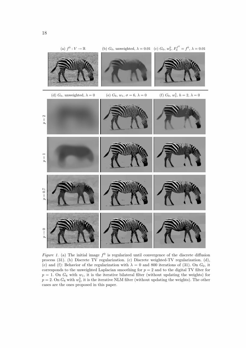
(a) f0 : V → R (b) G0, unweighted, λ = 0.01 (c) G0, w02 , F

f0

0= f0, λ = 0.01

(d) G0, unweighted, λ = 0 (e) G8, w1, σ = 6, λ = 0 (f) G8, w5

2 , h = 2, λ = 0

p=

2p

=1

p=

0.7

p→

0

Figure 1. (a) The initial image f0 is regularized until convergence of the discrete diffusionprocess (31). (b) Discrete TV regularization. (c) Discrete weighted-TV regularization. (d),(e) and (f): Behavior of the regularization with λ = 0 and 800 iterations of (31). On G0, itcorresponds to the unweighted Laplacian smoothing for p = 2 and to the digital TV filter forp = 1. On G8 with w1, it is the iterative bilateral filter (without updating the weights) forp = 2. On G8 with w5

2 , it is the iterative NLM filter (without updating the weights). The othercases are the ones proposed in this paper.

19

Part of 5th row of Fig. 1 in false colors Part of 6th row of Fig. 1 in false colorsp

=0.7

p→

0

Figure 2. Results presented in Fig. 1 for p < 1 and rendered here in false colors (each colorcorresponds to a gray value). We can observe the relation between the size of the neighborhoodand the leveling of the image.

of the neighborhood of the graph cannot be greater than one to preserve thediscontinuities. By using a weighted graph, we obtain the weighted-TV digitalfilter, which can be local, semilocal or nonlocal, depending on the weight func-tion. The difference between the weighted and unweighted cases is illustratedin Fig. 1(b) and 1(c) on the graph G0, and until convergence of the diffusion.We can observe that for the same value of λ, using a weight function helps topreserve the image discontinuities.

In order to compare the results with the particular cases described above, wegive examples of the proposed regularization, for several values of p, and theweight functions w1 and w2.

f0 : Z2 → R

3 Gaussian noise (σ = 20) G5, w32 , p = 0.7

Figure 3. Denoising of a color image by nonlocal regularization with 4 iterations and λ = 0.01.

Image smoothing/denoising. The behavior of the proposed regularization isillustrated in Fig. 1(d), 1(e) and 1(f) on an intensity image, for several valuesof p, several graph structures and λ = 0 (without the approximation term). Thenumber of iterations is the same for all the cases (800). We can do two principalobservations. The size of neighborhood of the graph helps to preserve sharp edgesand image redundancies, as well as the use of nonlocal weights. Also, when p < 1and particularly when p → 0, the regularization behaves like a simplificationprocedure. This last observation is depicted in the first row of Fig. 2, wherewe can see the effect of the structure of the graph. The local case (with G0),

20

which is computed efficiently, could be used in simplification and segmentationprocesses. The denoising of a color image is illustrated in Fig. 3 using a nonlocalrepresentation with p = 0.7. In our experiments, we found that using p < 1 inthe regularization process, with a local or a nonlocal representations, helps topreserve sharp edges.

Image simplification. Another way to simplify an image is to work on a moreabstract representation than adjacency or neighborhood graphs. One possiblerepresentation is obtained by constructing a fine partition (or over-segmentation)of the image and by considering neighborhood relations between the regions. Itis generally the first step of segmentation schemes and it provides a reduction ofthe number of elements to be analyzed by other processing methods. To computethe fine partition, many methods have been proposed, such as the ones basedon morphological operators (Meyer, 2001) or graph cut techniques and randomwalks (Meila and Shi, 2000). Here, we present a method that uses a graph-basedversion of the generalized Voronoi diagram presented by (Arbelaez and Cohen,2004). The initial image to be simplify is represented by a graph Gk = (V,E),k = 0 or 1, and a function f : V → R

m, as described previously.A path c(u, v) is a sequence of vertices (v1, . . . , vm) such that u = v1, v = vm,

and (vi, vi+1) ∈ E for all 1 ≤ i < m. Let CG(u, v) be the set of paths connectingu and v. We define the pseudo-metric µ : V × V → R

+ to be:

µ(u, v) = minc∈CG(u,v)

(m−1∑

i=1

‖dw(f)(vi, vi+1)‖)

,

where dw is the difference operator (4) defined in Section 2.2. Given a finite setof source vertices S = s1, . . . , sk ⊂ V , the energy induced by µ is given by theminimal individual energy:

µS(u) = infsi∈S

µ(si, u), ∀u ∈ V .

Based on the pseudo-metric µ, the influence zone of a source vertex si is definedto be the set of vertices of V that are closer to si than to any other source vertexof S:

Zµ(si, S, V ) = u ∈ V : µ(si, u) ≤ µ(sj, u), ∀sj ∈ S.The energy partition of the graph G, with respect to the set of sources S andthe pseudo-metric µ, corresponds to the set of influence zones:

Eµ(S,G) = Zµ(si, S, V ), ∀si ∈ S.

With these definitions, the image pre-segmentation consists in finding a set ofsource vertices and a pseudo-metric. We use the set of extrema of the intensity ofthe function f as a set of source vertices. To obtain exactly an energy partitionwhich considers the total variation of f along a path, we use dw(f)(u, v) = f(v)−

21

(a) original image f0 : V → R (b) region map (c) fine partition

(d) RAG (e) λ = 0.5 (f) λ = 0

Figure 4. Illustration of image simplification. First row: construction of the fine partition byenergy partition. The information in the fine partition is 8 percent of the one in the originalimage. Second row: regularization of the fine partition on the RAG with p = 2, w0

2 with

F f0 = f , and 30 iterations.

f(u) in the pseudo-metric. Then, the energy partition of the graph represents anapproximation of the image, by assigning a model to each influence zone of thepartition. The model is determined by the distribution of the graph values on theinfluence zone. Among the different models, the simplest are the constant ones,as mean or median value of the influence zone. The resultant graph G′ = (V ′, E ′)is a connectivity graph where V ′ = S and E ′ is the set of edges connecting twovertices si, sj ∈ S if there exists a vertex of Zµ(si, S, V ) connected to a vertexof Zµ(sj , S, V ). This last graph is known as the region adjacency graph (RAG)of the partition. Therefore, image simplification can be performed on the RAG(or a more complex neighborhood graph) and so the graph regularization canbe computed much faster relatively to classical images. The acceleration factordepends on the fineness of the partition and on the considered graph.

A result of the simplification process is illustrated in Fig. 4 on an image ofintensity. Fig. 4(b) represents the partition in random colors, and Fig. 4(c) thereconstructed image from the computed influence zones by assigning the meanintensity to modelize each zone. In our experiments, we found that the reductionof the information is at least of 90 percent. As illustrated in Fig. 4(e) and (f), thesimplification scheme can be carried on by regularizing the value of the zones on

22

the RAG associated to the fine partition. This simplification scheme has shownits effectiveness in the context of image segmentation, with other methods toconstruct the fine partition (Lezoray et al., 2007).

5.3. Application to polygonal mesh processing

By nature, polygonal curves and surfaces have a graph structure. Let V be theset of mesh vertices, and let E be the set of mesh edges. If the input mesh is noisy,we can regularize vertex coordinates or any other function f 0 : V ⊂ R

n → Rm

defined on the graph G = (V,E, w).

f0 : V ⊂ R2 → R

2 p = 2, λ = 0 p = 2, λ = 0.25

Figure 5. Polygonal curve denoising by diffusion of the position of the vertices. The polygonsedges are unweighted. In the case of λ = 0 shrinkage effects are introduced (30 iterations). Thecase of λ > 0 (100 iterations) helps to avoid these undesirable effects.

Mesh denoising. The discrete regularization can be used to smooth and denoisepolygonal meshes. As in image processing, denoising a polygonal curve or surfaceconsist in removing spurious details while preserving geometric features. Thereexists two common frameworks in the literature to do this. The first one considersthe position of the vertices as the function to be processed. The second oneconsists in regularizing the normals direction at the mesh vertices.

We illustrate the first scheme in order to show the importance of using thefitting term in regularization processes, which is not commonly used in meshprocessing. This is illustrated Fig. 5 on a polygonal curve. One can observe thatthe regularization performed using the fitting term (λ > 0) helps to avoid theshrinkage effects obtained without using the fitting term (λ = 0), and whichcorresponds to the Laplacian smoothing (Taubin, 1995). The regularization ofpolygonal surfaces is illustrated in Fig. 6. Here again, the fitting term helps toavoid shrinkage effects. On can remark that we use the discrete diffusion (31),which is not the classical algorithm to perform Laplacian smoothing in mesh pro-cessing. Most of the methods are based on the algorithm (24) with λ = 0 (Taubin,1995; Desbrun et al., 2000; Xu, 2004). The proposed p-Laplacian diffusion, whichextends the Laplacian diffusion, is described next for p < 1.

23

(a) original mesh (b) normal noise (c) p = 2, λ = 0.5

Figure 6. Mesh denoising. (a) Original Stanford Bunny with |V | = 35949. (b) Noisy Bunnywith normal noise. (c) Regularization of vertex coordinates on the graph (8 iterations of thediffusion process and w(u, v) = 1/‖u− v‖2

2).

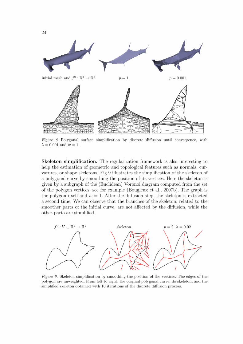
Curve and surface simplification. As in the case of images, when p < 1the regularization process can be seen as a clustering method. This is illustratedin Fig. 7 on a polygonal curve, and in Fig. 8 on a polygonal surface. One canobserve that when p → 0, the vertices aggregates. Also, the global shape of thecurve is preserved, as well as the discontinuities, without important shrinkageeffects. This provides a new way of simplifying meshes.

f0 : R2 → R

2 p = 0.01, t = 10 p = 0.01, t = 100

bb

b b bbbbbbb

bb

b bb bbbbbbbbbbbbb

b

bbbbbbbbbbbbbbbbbbbbbbbbbbbbbbbbbbbbbbbbbbbbbbbb

bbbbb

b

bb

bb

bbb

bbbbb

bbbb

bbbb

bbbbb

bbbbbb

bbbbb

bbbb

b

bbbbbbbbbbb

bb

bbbbbbbbbb

bbbbbbb

bbb

bbbbbbbbbb b b b b b b b b bbbbbb

bbbb

b

b

b

bbbb

bb

bb

bb

bb

b

bbbb

bbb

bbbbbbbbbbbbbbbbbbbbb

bbbbbbbb bbbbbb

bbbb

bbb b

b

bb

bb

bbb

bbbbbbbbbbb

b

bbbbbbbbbbbb

bbb

b

bbbbbbbbbbbbbbbbbbbbbbbbbbbbbbbbbbbbbbb

b

bbbbbbbbbb

b

bb

b

bb

b

bbbb

b

bbbb

bbbb

bbbb

bbbbb

bbbbbbbbb

bb

bbbb

b

bbbbbbbbbbbbb

bbbbbbbbbbbbbbbbb

b

b

bbbbbbbbbbb bbbbb b bbbbb

bbbbbbbb

b

b

bbbbb

bbb

bb

bb

bbbbbbbb

bbbbbbbbbbbbbbbbbbbbb

bbbbbbbbbbbbbbbb bb

bbb b

b

bb

bb

b

bbbb

b

bbbb

bbbbb

bbbbb

bbbbbbbbbb

b

bbbbbbbbbbbb

bbbbbbb

bbbbbb

bbbbbbb

bbbbbbb

bbbbbbb

bbbb

bbb

b

bb

bbbbb

bbbbb

bbbbb

bbbbbbbbbbbbbbbbb

bbbbbb

bbbbbbb

bbbbbbb

bbbbbbbbbbbbb

bbbbb

bbbbbbb

bbbb

bbbbbbb bbbbb

bbbbbbbb

bb

bbbbb

bb

bbb

bb

bbbbb

b

b

b

bbbbbbbbbbbbbbbbbbbbb

bbbbbbbbbbbbbbbbbb

bbbb

b

bb

bbb

Figure 7. Polygonal curve simplification by regularization of the position of the vertices (withp < 1). The graph is the polygon itself, and w = 1. First row: the vertices. Second row: theassociated processed polygons.

24

initial mesh and f0 : R3 → R

3 p = 1 p = 0.001

Figure 8. Polygonal surface simplification by discrete diffusion until convergence, withλ = 0.001 and w = 1.

Skeleton simplification. The regularization framework is also interesting tohelp the estimation of geometric and topological features such as normals, cur-vatures, or shape skeletons. Fig.9 illustrates the simplification of the skeleton ofa polygonal curve by smoothing the position of its vertices. Here the skeleton isgiven by a subgraph of the (Euclidean) Voronoi diagram computed from the setof the polygon vertices, see for example (Bougleux et al., 2007b). The graph isthe polygon itself and w = 1. After the diffusion step, the skeleton is extracteda second time. We can observe that the branches of the skeleton, related to thesmoother parts of the initial curve, are not affected by the diffusion, while theother parts are simplified.

f0 : V ⊂ R2 → R

2 skeleton p = 2, λ = 0.02

Figure 9. Skeleton simplification by smoothing the position of the vertices. The edges of thepolygon are unweighted. From left to right: the original polygonal curve, its skeleton, and thesimplified skeleton obtained with 10 iterations of the discrete diffusion process.

25

6. Conclusion

We propose a general discrete framework for regularizing real-valued or vector-valued functions on weighted graphs of arbitrary topology. The regularization,based on a discrete p-Dirichlet energy, leads to a family of nonlinear iterativeprocesses which includes several filters used in image and mesh processing.

The choice of the graph topology and the choice of the weight function allowto regularize any discrete data set or any function defined on a discrete dataset. Indeed, the data can be structured by neighborhood graphs weighted byfunctions depending on data features. This can be applied in the context of imagesmoothing, denoising or simplification. We also show that local and nonlocalregularization functionals have the same expression when defined on graphs.The main ongoing work is to use the proposed framework in the context ofhierarchical mesh segmentation and point cloud clustering.

Appendix

A. Proofs of Section 2

Proof of Proposition 1: From the expressions of the inner product in H(E)(Eq. (2)) and the difference operator, the left side of Eq. (6) is written as:

〈H, dwf〉H(E) =∑

xy∈E

H(xy) (γyxf(y) − γxyf(x))

=∑

xy∈E

γyxH(xy)f(y)−∑

xy∈E

γxyH(xy)f(x).

By replacing∑

xy∈E by∑

x∈V

∑y∼x, and x and y by u and v, we have:

〈H, dwf〉H(E) =∑

u∈V

∑

v∼u

γuvH(v, u)f(u)−∑

u∈V

∑

v∼u

γuvH(u, v)f(u)

=∑

u∈V

f(u)∑

v∼u

γuv (H(v, u)−H(u, v)) (32)

(6)= 〈d∗wH, f〉H(V )

(1)=∑

u∈V

d∗w(H)(u)f(u). (33)

Then, the result is obtained from Eq. (32) and Eq. (33) by taking f(u) = 1, forall u ∈ V .

Proof of Proposition 2: From the definition of the p-Laplace operator (Eq. (11)),and the expression of the difference operator and its adjoint (Proposition 1), we

26

have:

∆pwf(u) =

∑

v∼u

γuv

(| w f(v)|p−2dw(f)(v, u)− | w f(u)|p−2dw(f)(u, v)

)

=∑

v∼u

γuv

(| w f(v)|p−2 + | w f(u)|p−2

)dw(f)(v, u).

Now, we show that Eq. (13) is equal to Eq. (12), using the definition of the edgederivative (Eq. (5)):

(13) =∑

v∼ue=(u,v)

γuv

(γvu| w f(v)|p−2

γvu

∂f

∂e

∣∣∣∣v

− γuv| w f(u)|p−2

γuv

∂f

∂e

∣∣∣∣u

)

=∑

v∼ue=(u,v)

γuv

(| w f(v)|p−2(γuvf(u) − γvuf(v))

−| w f(u)|p−2(γvuf(v) − γuvf(u)))

= (12).

B. Proof of Section 3

Proof of Property 2: The partial derivative of Rp-TVw (f), at a vertex u1 ∈ V is

given by:

∂

∂f

(∑

u∈V

| w f(u)|p)∣∣∣∣∣

u1

(9)=

∂

∂f

∑

u∈V

(∑

v∼u

(γvuf(v) − γuvf(u))2)p

2

∣∣∣∣∣∣u1

.

(34)The derivative depends only on the edges incident to u1. Let v1, . . . , vk be thevertices of V connected to u1 by an edge of E. Then we have:

(34) = −p∑

v∼u1

γu1v (γvu1f(v) − γu1vf(u1))

(∑

v∼u1

(γvu1f(v) − γu1vf(u1))

2

) p−2

2

+ pγu1v1(γu1v1

f(u1) − γv1u1f(v1))

(∑

v∼v1

(γvv1f(v) − γv1vf(v1))

2

) p−2

2

+ . . .+ pγu1vk(γu1vk

f(u1) − γvku1f(vk))

(∑

v∼vk

(γvvkf(v) − γvkvf(vk))

2

) p−2

2

(9)= p

∑

v∼u1

γu1v (γu1vf(u1) − γvu1f(v)) | w f(u1)|p−2

+ p∑

v∼u1

γu1v (γu1vf(u1) − γvu1f(v)) | w f(v)|p−2 (12)

= p∆pwf(u1).

27

References

Alvarez, L., F. Guichard, P.-L. Lions, and J.-M. Morel: 1993, ‘Axioms and fundamentalequations of image processing’. Archive for Rational Mechanics and Analysis 123(3),199–257.

Arbelaez, P. A. and L. D. Cohen: 2004, ‘Energy Partitions and Image Segmentation’. Journalof Mathematical Imaging and Vision 20(1-2), 43–57.

Aubert, G. and P. Kornprobst: 2006, Mathematical Problems in Image Processing, PartialDifferential Equations and the Calculus of Variations, No. 147 in Applied MathematicalSciences. Springer, 2nd edition.

Bajaj, C. L. and G. Xu: 2003, ‘Anisotropic diffusion of surfaces and functions on surfaces’.ACM Trans. on Graph. 22(1), 4–32.

Barash, D.: 2002, ‘A Fundamental Relationship between Bilateral Filtering, Adaptive Smooth-ing, and the Nonlinear Diffusion Equation’. IEEE Trans. Pattern Analysis and MachineIntelligence 24(6), 844–847.

Bensoussan, A. and J.-L. Menaldi: 2005, ‘Difference Equations on Weighted Graphs’. Journalof Convex Analysis 12(1), 13–44.

Bobenko, A. I. and P. Schroder: 2005, ‘Discrete Willmore Flow’. In: M. Desbrun and H.Pottmann (eds.): Eurographics Symposium on Geometry Processing. pp. 101–110.

Bougleux, S. and A. Elmoataz: 2005, ‘Image Smoothing and Segmentation by Graph Regu-larization.’. In: Proc. Int. Symp. on Visual Computing (ISVC), Vol. 3656 of LNCS. pp.745–752, Springer.

Bougleux, S., A. Elmoataz, and M. Melkemi: 2007a, ‘Discrete Regularization on WeightedGraphs for Image and Mesh Filtering’. In: F. Sgallari, A. Murli, and N. Paragios (eds.):Proc. of the 1st Int. Conf. on Scale Space and Variational Methods in Computer Vision(SSVM), Vol. 4485 of LNCS. pp. 128–139, Springer.

Bougleux, S., M. Melkemi, and A. Elmoataz: 2007b, ‘Local Beta-Crusts for Simple CurvesReconstruction’. In: C. M. Gold (ed.): 4th International Symposium on Voronoi Diagramsin Science and Engineering (ISVD’07). pp. 48–57, IEEE Computer Society.

Brox, T. and D. Cremers: 2007, ‘Iterated Nonlocal Means for Texture Restoration’. In: F.Sgallari, A. Murli, and N. Paragios (eds.): Proc. of the 1st Int. Conf. on Scale Space andVariational Methods in Computer Vision (SSVM), Vol. 4485 of LNCS. pp. 12–24, Springer.

Buades, A., B. Coll, and J.-M. Morel: 2005, ‘A review of image denoising algorithms, with anew one’. Multiscale Modeling and Simulation 4(2), 490–530.

Chambolle, A.: 2005, ‘Total Variation Minimization and a Class of Binary MRF Models’. In:Proc. of the 5th Int. Work. EMMCVPR, Vol. 3757 of LNCS. pp. 136–152, Springer.

Chan, T., S. Osher, and J. Shen: 2001, ‘The Digital TV Filter and Nonlinear Denoising’. IEEETrans. Image Processing 10(2), 231–241.

Chan, T. and J. Shen: 2005, Image Processing and Analysis - variational, PDE, wavelets, andstochastic methods. SIAM.

Chung, F.: 1997, ‘Spectral Graph Theory’. CBMS Regional Conference Series in Mathematics92, 1–212.

Clarenz, U., U. Diewald, and M. Rumpf: 2000, ‘Anisotropic geometric diffusion in surfaceprocessing’. In: VIS’00: Proc. of the conf. on Visualization. pp. 397–405, IEEE ComputerSociety Press.

28

Coifman, R., S. Lafon, A. Lee, M. Maggioni, B. Nadler, F. Warner, and S. Zucker: 2005,‘Geometric diffusions as a tool for harmonic analysis and structure definition of data’.Proc. of the National Academy of Sciences 102(21).

Coifman, R., S. Lafon, M. Maggioni, Y. Keller, A. Szlam, F. Warner, and S. Zucker: 2006,‘Geometries of sensor outputs, inference, and information processing’. In: Proc. of the SPIE:Intelligent Integrated Microsystems, Vol. 6232.

Cvetkovic, D. M., M. Doob, and H. Sachs: 1980, Spectra of Graphs, Theory and Application,Pure and Applied Mathematics. Academic Press.

Darbon, J. and M. Sigelle: 2004, ‘Exact Optimization of Discrete Constrained Total VariationMinimization Problems’. In: R. Klette and J. D. Zunic (eds.): Proc. of the 10th Int.Workshop on Combinatorial Image Analysis, Vol. 3322 of LNCS. pp. 548–557.

Desbrun, M., M. Meyer, P. Schroder, and A. Barr: 2000, ‘Anisotropic Feature-PreservingDenoising of Height Fields and Bivariate Data’. Graphics Interface pp. 145–152.

Fleishman, S., I. Drori, and D. Cohen-Or: 2003, ‘Bilateral mesh denoising’. ACM Trans. onGraphics 22(3), 950–953.

Friedman, J. and J.-P. Tillich: 2004, ‘Wave equations for graphs and the edge-based laplacian’.Pacific Journal of Mathematics 216(2), 229–266.

Gilboa, G. and S. Osher: 2007a, ‘Nonlocal linear image regularization and supervisedsegmentation’. SIAM Multiscale Modeling and Simulation 6(2), 595–630.

Gilboa, G. and S. Osher: 2007b, ‘Nonlocal Operators with Applications to Image Processing’.Technical Report 07-23, UCLA, Los Angeles, USA.

Griffin, L. D.: 2000, ‘Mean, Median and Mode Filtering of Images’. Proceedings: Mathematical,Physical and Engineering Sciences 456(2004), 2995–3004.

Hildebrandt, K. and K. Polthier: 2004, ‘Anisotropic Filtering of Non-Linear Surface Features’.Eurographics 2004: Comput. Graph. Forum 23(3), 391–400.

Jones, T. R., F. Durand, and M. Desbrun: 2003, ‘Non-iterative, feature-preserving meshsmoothing’. ACM Trans. Graph. 22(3), 943–949.

Kervrann, C., J. Boulanger, and P. Coupe: 2007, ‘Bayesian non-local means filter, imageredundancy and adaptive dictionaries for noise removal’. In: F. Sgallari, A. Murli, andN. Paragios (eds.): Proc. of the 1st Int. Conf. on Scale Space and Variational Methods inComputer Vision (SSVM), Vol. 4485 of LNCS. pp. 520–532, Springer.

Kimmel, R., R. Malladi, and N. Sochen: 2000, ‘Images as embedding maps and minimalsurfaces: Movies, color, texture, and volumetric medical images’. International Journalof Computer Vision 39(2), 111–129.

Kinderman, S., S. Osher, and S. Jones: 2005, ‘Deblurring and denoising of images by nonlocalfunctionals’. SIAM Multiscale Modeling and Simulation 4(4), 1091–1115.

Lee, J. S.: 1983, ‘Digital Image Smoothing and the Sigma Filter’. Computer Vision, Graphics,and Image Processing 24(2), 255–269.

Lezoray, O., A. Elmoataz, and S. Bougleux: 2007, ‘Graph regularization for color imageprocessing’. Computer Vision and Image Understanding 107(1-2), 38–55.

Meila, M. and J. Shi: 2000, ‘Learning segmentation by random walks’. Advances in NeuralInformation Processing Systems 13, 873–879.

Meyer, F.: 2001, ‘An overview of morphological segmentation’. International Journal of PatternRecognition and Artificial Intelligence 15(7), 1089–1118.

Mrazek, P., J. Weickert, and A. Bruhn: 2006, ‘On robust estimation and smoothing with spatialand tonal kernels’. In: Geometric Properties from Incomplete Data, Vol. 31 of ComputationalImaging and Vision. pp. 335–352, Springer.

Osher, S. and J. Shen: 2000, ‘Digitized PDE method for data restoration’. In: E. G. A.Anastassiou (ed.): In Analytical-Computational methods in Applied Mathematics. Chap-man&Hall/CRC, pp. 751–771.

29

Paragios, N., Y. Chen, and O. Faugeras (eds.): 2005, Handbook of Mathematical Models inComputer Vision. Springer.

Paris, S., P. Kornprobst, J. Tumblin, and F. Durand: 2007, ‘A gentle introduction to bilateralfiltering and its applications’. In: SIGGRAPH ’07: ACM SIGGRAPH 2007 courses. ACM.

Peyre, G.: 2008, ‘Image processing with non-local spectral bases’. to appear in SIAM MultiscaleModeling and Simulation.

Requardt, M.: 1997, ‘A New Approach to Functional Analysis on Graphs, the Connes-SpectralTriple and its Distance Function’.

Shi, J. and J. Malik: 2000, ‘Normalized cuts and image segmentation’. IEEE Transactions onPattern Analysis and Machine Intelligence 22(8), 888–905.

Smith, S. and J. Brady: 1997, ‘SUSAN - a new approach to low level image processing’.International Journal of Computer Vision (IJCV) 23, 45–78.

Sochen, N., R. Kimmel, and A. M. Bruckstein: 2001, ‘Diffusions and Confusions in Signal andImage Processing’. Journal of Mathematical Imaging and Vision 14(3), 195–209.

Szlam, A. D., M. Maggioni, and R. R. Coifman: 2006, ‘A General Framework for Adap-tive Regularization Based on Diffusion Processes On Graphs’. Technical ReportYALE/DCS/TR1365, YALE.

Tasdizen, T., R. Whitaker, P. Burchard, and S. Osher: 2003, ‘Geometric surface processing vianormal maps’. ACM Trans. on Graphics 22(4), 1012–1033.

Taubin, G.: 1995, ‘A signal processing approach to fair surface design’. In: SIGGRAPH’95:Proc. of the 22nd Annual Conference on Computer Graphics and Interactive Techniques.pp. 351–358, ACM Press.

Tomasi, C. and R. Manduchi: 1998, ‘Bilateral Filtering for Gray and Color Images’. In:ICCV’98: Proc. of the 6th Int. Conf. on Computer Vision. pp. 839–846, IEEE ComputerSociety.

Weickert, J.: 1998, Anisotropic Diffusion in Image Processing, ECMI series. Teubner-Verlag.Xu, G.: 2004, ‘Discrete Laplace-Beltrami operators and their convergence’. Computer Aided

Geometric Design 21, 767–784.Yagou, H., Y. Ohtake, and A. Belyaev: 2002, ‘Mesh smoothing via mean and median filtering

applied to face normals’. In: Proc. of the Geometric Modeling and Processing (GMP’02) -Theory and Applications. pp. 195–204, IEEE Computer Society.

Yoshizawa, S., A. Belyaev, , and H.-P. Seidel: 2006, ‘Smoothing by example: mesh denoisingby averaging with similarity-based weights’. In: Proc. International Conference on ShapeModeling and Applications. pp. 38–44.

Zhou, D. and B. Scholkopf: 2005, ‘Regularization on Discrete Spaces’. In: Proc. of the 27thDAGM Symp., Vol. 3663 of LNCS. pp. 361–368, Springer.