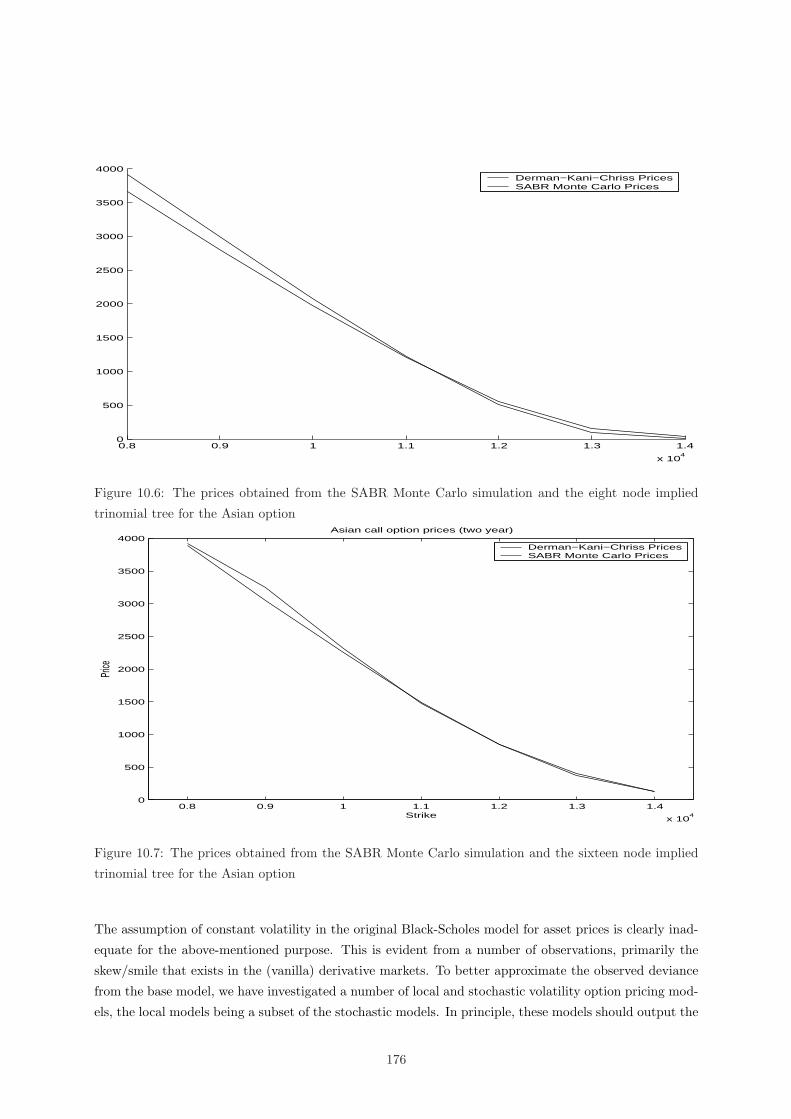
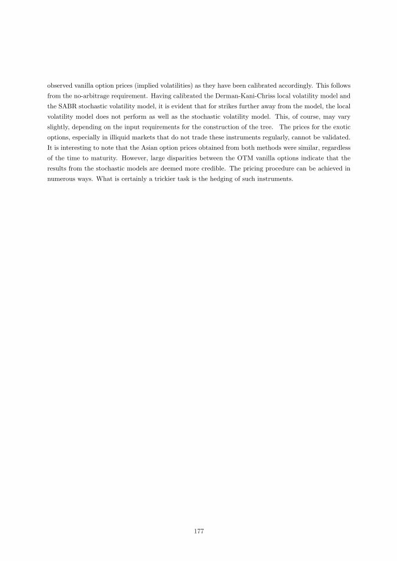
Local and Stochastic Volatility Models: An Investigation into the Pricing of Exotic Equity Options A dissertation submitted to the Faculty of Science, University of the Witwatersrand, Johannesburg, South Africa, in fulfillment of the requirements of the degree of Master of Science. Abstract The assumption of constant volatility as an input parameter into the Black-Scholes option pricing formula is deemed primitive and highly erroneous when one considers the terminal distribution of the log-returns of the underlying process. To account for the ‘fat tails’ of the distribution, we consider both local and stochastic volatility option pricing models. Each class of models, the former being a special case of the latter, gives rise to a parametrization of the skew, which may or may not reflect the correct dynamics of the skew. We investigate a select few from each class and derive the results presented in the corresponding papers. We select one from each class, namely the implied trinomial tree (Derman, Kani & Chriss 1996) and the SABR model (Hagan, Kumar, Lesniewski & Woodward 2002), and calibrate to the implied skew for SAFEX futures. We also obtain prices for both vanilla and exotic equity index options and compare the two approaches. Lisa Majmin September 29, 2005
Transcript
Local and Stochastic Volatility Models: An Investigation into the
Pricing of Exotic Equity Options
A dissertation submitted to the Faculty of Science, University of the Witwatersrand, Johannesburg, South
Africa, in fulfillment of the requirements of the degree of Master of Science.
Abstract
The assumption of constant volatility as an input parameter into the Black-Scholes option pricing
formula is deemed primitive and highly erroneous when one considers the terminal distribution of the
log-returns of the underlying process. To account for the ‘fat tails’ of the distribution, we consider
both local and stochastic volatility option pricing models. Each class of models, the former being
a special case of the latter, gives rise to a parametrization of the skew, which may or may not
reflect the correct dynamics of the skew. We investigate a select few from each class and derive the
results presented in the corresponding papers. We select one from each class, namely the implied
trinomial tree (Derman, Kani & Chriss 1996) and the SABR model (Hagan, Kumar, Lesniewski &
Woodward 2002), and calibrate to the implied skew for SAFEX futures. We also obtain prices for
both vanilla and exotic equity index options and compare the two approaches.
Lisa Majmin
September 29, 2005
I declare that this is my own, unaided work. It is being submitted for the Degree of Master of Science to
the University of the Witwatersrand, Johannesburg. It has not been submitted before for any degree or
examination to any other University.
(Signature)
(Date)
I would like to thank my supervisor, mentor and friend Dr Graeme West for his guidance, dedication and
his persistent effort. I would also like to give thanks to Professors D.P. Mason and P.S. Hagan as well as
Grant Lotter for their additional assistance and to the heads of department, Professors D. Sherwell and
D. Taylor.
I owe my deepest gratitude to my parents for their unconditional support and kindness.
i
Contents
1 Introduction 1
2 Local Volatility Models: Implied Binomial and Trinomial Trees 4
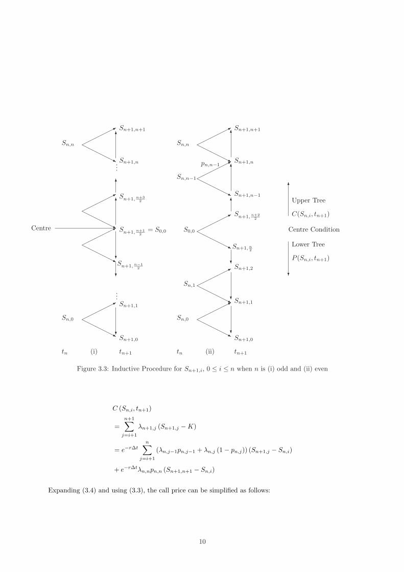
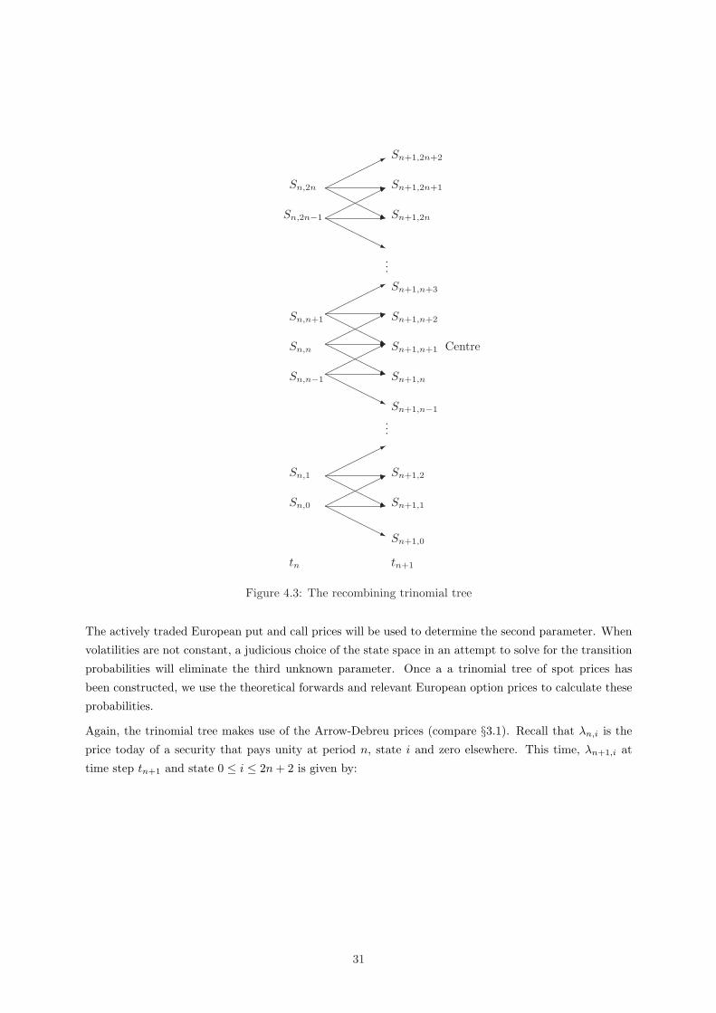
The last line follows from a substitution of ∆Ci . The node just below the centre, Sn,i for i = n
2 , can
be solved for according to
Sn+1,i =fn,i
(λn,ifn,i −∆C
i
)
λn,ifn,i + ∆Ci
So, if the number of nodes is either even or odd, the centring condition gives rise to the remainder
of the nodes of the tree.
4. Negative Transition Probabilities
In (Derman & Kani 1994), the problem of obtaining transition probabilities that indicated an
arbitrage opportunity was dealt with by maintaining the logarithmic spacing between adjacent
nodes equal to that of the previous level. Yet, this may still be violating the inequality fn,i ≤Sn+1,i+1 ≤ fn,i+1. To avoid this, a choice of any point between fn,i and fn,i+1 is sufficient. Simply
choose the average of the two forwards.
22
3.7.1 Non-Constant Time Intervals and a Dividend Yield
If it is the case that the input data (option expiry times) is not equally spaced, the resulting binomial
tree should display such a feature. The original Derman-Kani algorithm will not be able to allow for
direct modification, as the option prices used to determine the tree of spot prices are calculated using a
binomial tree approach. One would have to perform interpolation to obtain the required data at equally
spaced dates.
A dividend yield can easily be accounted for by slightly modifying the theoretical forward prices (and
European option prices) calculated. At node (n, i), the forward price with a dividend yield q is given by:
fn,i = Sn,ie(r−q)∆t.
In the Barle & Cakici algorithm, the additional inputs required are all the options’ expiries. The above
procedure is modified by replacing the constant ∆t with the relevant time interval. Given N option expiry
times and a total time period of T , for non-constant time intervals, we have that
T =N∑
i=1
∆ti,
where ∆ti = ti − ti−1. Therefore, the forward price at node (n, i) is given by
fn,i = Sn,ie(r−q)∆ti+1 .
3.8 Discrete Dividends and a Term Structure of Interest Rates
(Brandt & Wu 2002) suggest two further modifications to the original algorithm to incorporate discrete
dividends and to allow for a non-constant interest rate. The centring condition and the strikes of the
European options are those suggested in (Barle & Cakici 1995) as this ensures the phenomenon of negative
probabilities associated with the nodes is eliminated from the middle section of the tree. Thus, the
economically interesting region of the tree is unaffected.
Once again, the N nodes of the tree are equally spaced ∆t apart, where ∆t = TN , T being the final
maturity. The construction of the tree is identical to that proposed by Derman and Kani. Assuming all
information has been evaluated up to time step tn, that is:
• Sn,i
• λn,i are known for nodes (n, i), 0 ≤ i ≤ n
Consider the upper portion of the tree:
For each Sn,i, the movement is to Sn+1,i+1 with probability pn,i and to Sn+1,i with probability 1− pn,i,
for n+12 ≤ i ≤ n + 1 if n is odd, or n
2 + 1 ≤ i ≤ n + 1 if n is even. Assume Sn+1,i is known and as before,
fn,i denotes the price at node (n, i) of a forward contract with maturity date tn+1.
Solve for Sn+1,i+1 as follows:
23
• Risk-neutrality of the tree implies:
fn,i = pn,iSn+1,i+1 + (1− pn,i)Sn+1,i
So,
pn,i =fn,i − Sn+1,i
Sn+1,i+1 − Sn+1,i
• The theoretical forward price with discrete dividends is:
fn,i = Sn,iern+1∆t −Dn+1 (3.21)
where rn+1 denotes the interest rate applicable between tn and tn+1 and Dn+1 is the discrete
dividend with ex-dividend date tn+1. If the dividends are paid in-between nodes, the tree is adjusted
by paying the forward value of the dividends at the nodes following the ex-dividend dates.
Let ci(K, tn+1) denote the price at node (n, i) of a ‘one step ahead’ European call option that matures
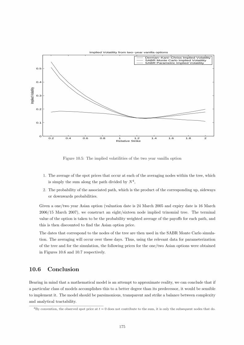
The input data, which is identical to the case of the implied binomial tree in Chapter 3, is required for
the specification of the state space.
1. Valuation date (taken to be t = 0)
43
2. Spot on valuation date
3. Expiry dates of all European options
4. Futures (or forward) level corresponding to the valuation date; if this is not provided, the algorithm
uses the theoretical forward rates1
5. Risk-free rate
6. Dividend yield
7. Implied volatilities for various strikes relevant at each time step tj for 1 ≤ j ≤ N where tN = T
8. The number of time steps in the implied tree N - this does not necessarily have to agree with N .
9. Specification of the nature of the input:
(I) No extreme term or skew structure, normal trinomial state space.
(II) Term Structure: State space with unequal time steps.
(III) Skew Structure: Require ATM implied volatility, slope of the linear function to construct a
state space with nodal spacing that varies vertically.
(IV) Both: A skewed state space is first constructed, followed by a term structure.
4.6.2 Constructing the required state space
Case I: Normal State Space
In this case, there is no extreme term or skew structure associated with the local volatility function. An
underlying constant-volatility trinomial tree will be appropriate for the determination of the transition
probabilities and Arrow-Debreu prices. A single time step of the trinomial tree is constructed from the
combination of two steps of the binomial Cox-Ross-Rubinstein tree.
Consider the Cox-Ross-Rubinstein constant volatility trinomial tree2:1We will be pricing European and some path-dependent options on the ALSI40 equity index. Most relevant information
is provided by implied skew data (from the South African Futures Exchange, SAFEX, or a dealer) on the futures contracts
on this index that trade. It is also convenient for interpolation purposes as the ATM implied volatility can be found using
raw interpolation on the relative strikes, this is X/F , where X is the strike and F is the ATM futures level.2Since two steps of a binomial C-R-R tree equates to one step of the C-R-R trinomial tree, then Su2 = SU and Sd2 = SD,
where u = eσq
∆t2 is the upward movement in a binomial tree of time step ∆t
2and d = e
−σq
∆t2 the downward movement.
When one time step in the trinomial tree is ∆t, then U =“eσ√
∆t/2”2
= eσ√
2∆t, and similarly D = e−σ√
2∆t. Given that
the risk-neutral probability of an upward movement in the binomial tree over a time step ∆t2
is given by
π =er ∆t
2 − d
u− d
=er ∆t
2 − e−σq
∆t2
eσq
∆t2 − e
−σq
∆t2
,
then in the trinomial tree of time step ∆, the probabilities associated with the up, down and middle movements are given
by pU = p = π2, pD = q = (1− π)2 and pM = 1− pU − pD.
44
• Su = Seσ√
2∆t
• Sm = S
• Sd = Se−σ√
2∆t
• p =(
er∆t/2−e−σ√
∆t/2
eσ√
∆t/2−e−σ√
∆t/2
)2
• q =(
eσ√
∆t/2−er∆t/2
eσ√
∆t/2−e−σ√
∆t/2
)2
where S is the spot price at the current time step, p and q represent the transition probabilities of an
up and down movement respectively, σ is the constant volatility of an ATM option and Su, Sm and Sd
are the spot prices at the following time step. The movement is shown explicitly in Figure 4.2. The time
The probabilities, as stated above, will not be used. The required transition probabilities, pn,i, qn,i and
1− pn,i − qn,i, are what is required in the implied tree approach. The state space is a platform that can
be selected using the additional degree of freedom. This is a result of selecting a trinomial as opposed to
a binomial tree.
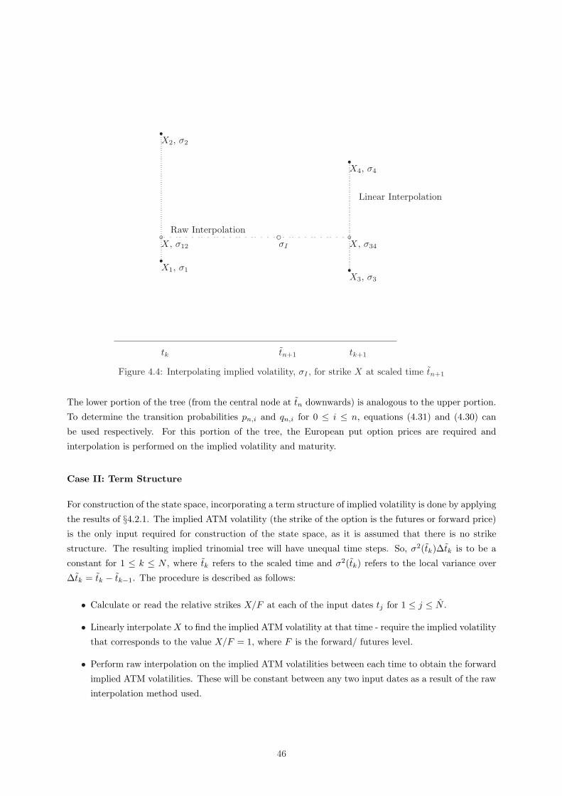
Consider the upper portion of the tree (from Sn+1,n+2 to Sn+1,2n+2) at t = tn+1: (4.27) and (4.28) are
used to calculate pn,i and qn,i for n+1 ≤ i ≤ 2n. For this part of the tree, the European call option prices
are required. Since there is a term structure of implied volatility and the constructed state space has
time intervals which will not always coincide with the input dates, it will be necessary to perform linear
interpolation in the vertical direction (on the strikes) and raw interpolation in the horizontal direction
(on the implied volatilities at a date that is not an input). See Figure 4.4. This is done to obtain the
implied volatility at a non-input strike for an option expiring at a non-input date. To ensure that forward
rates are always positive, the raw interpolation method is required.
Refer to Figure 4.4. To calculate the implied volatility, σI , for strike X and maturity tn+1, linear
interpolation is first performed on the implied volatilities σ1 and σ2 (which relates to strikes X1 and X2)
at maturity tk to obtain σ12. The next linear interpolation is performed on σ3 and σ4 at maturity tk+1
to obtain σ34. These implied volatilities relate to the strike X at maturities tk and tk+1.
Consider the calculation of σ12 and σ34:
σ12 =X −X1
X2 −X1σ2 +
X2 −X
X2 −X1σ1
σ34 =X −X3
X4 −X3σ4 +
X4 −X
X4 −X3σ3
Then, σI at tn+1 is calculated using by (4.20):
σI =
√tktk+1 (σ2
12(tk)− σ234(tk+1))
tn+1 (tk+1 − tk)+
σ234(tk+1)tk+1 − σ2
12(tk)tktk+1 − tk
.
Once the implied volatility has been evaluated, either a constant volatility trinomial tree or the Black-
Scholes formula can be used to price the option.
45
tk tk+1tn+1
Raw Interpolation
Linear Interpolation
X, σ12
bX, σ34
bσI
c
X1, σ1
r
X2, σ2
r
X3, σ3
r
X4, σ4
r
Figure 4.4: Interpolating implied volatility, σI , for strike X at scaled time tn+1
The lower portion of the tree (from the central node at tn downwards) is analogous to the upper portion.
To determine the transition probabilities pn,i and qn,i for 0 ≤ i ≤ n, equations (4.31) and (4.30) can
be used respectively. For this portion of the tree, the European put option prices are required and
interpolation is performed on the implied volatility and maturity.
Case II: Term Structure
For construction of the state space, incorporating a term structure of implied volatility is done by applying
the results of §4.2.1. The implied ATM volatility (the strike of the option is the futures or forward price)
is the only input required for construction of the state space, as it is assumed that there is no strike
structure. The resulting implied trinomial tree will have unequal time steps. So, σ2(tk)∆tk is to be a
constant for 1 ≤ k ≤ N , where tk refers to the scaled time and σ2(tk) refers to the local variance over
∆tk = tk − tk−1. The procedure is described as follows:
• Calculate or read the relative strikes X/F at each of the input dates tj for 1 ≤ j ≤ N .
• Linearly interpolate X to find the implied ATM volatility at that time - require the implied volatility
that corresponds to the value X/F = 1, where F is the forward/ futures level.
• Perform raw interpolation on the implied ATM volatilities between each time to obtain the forward
implied ATM volatilities. These will be constant between any two input dates as a result of the raw
interpolation method used.
46
Once all the forward implied ATM volatilities have been found, use (4.16) to solve for the scaled times by
induction. The necessary calculations are simplified due to the forward implied ATM volatilities being
constant.
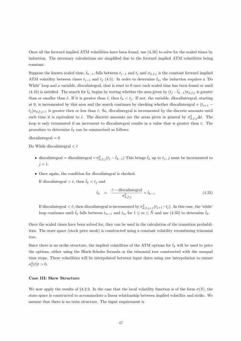
Suppose the known scaled time, tk−1, falls between tj−1 and tj and σd,f ;j is the constant forward implied
ATM volatility between times tj−1 and tj (4.5). In order to determine tk, the induction requires a ’Do
While’ loop and a variable, dlocalintegral, that is reset to 0 once each scaled time has been found or until
(4.16) is satisfied. The search for tk begins by testing whether the area given by (tj− tk−1)σd,f ;j is greater
than or smaller than c. If it is greater than c, then tk < tj . If not, the variable, dlocalintergral, starting
at 0, is incremented by this area and the search continues by checking whether dlocalintergral + (tj+1 −tj)σd,f ;j+1 is greater then or less than c. So, dlocalintegral is incremented by the discrete amounts until
such time it is equivalent to c. The discrete amounts are the areas given in general by σ2d,f ;j∆t. The
loop is only terminated if an increment to dlocalintegral results in a value that is greater than c. The
procedure to determine tk can be summerized as follows:
dlocalintegral = 0
Do While dlocalintegral < c
• dlocalintegral = dlocalintegral + σ2d,f ;j(tj − tk−1) This brings tk up to tj , j must be incremented to
j + 1.
• Once again, the condition for dlocalintegral is checked.
If dlocalintegral > c, then tk < tj and
tk =c− dlocalintegral
σ2d,f ;j
+ tk−1 (4.33)
If dlocalintegral < c, then dlocalintegral is incremented by σ2d,f ;j+1(tj+1−tj). In this case, the ’while’
loop continues until tk falls between tm−1 and tm for 1 ≤ m ≤ N and use (4.33) to determine tk.
Once the scaled times have been solved for, they can be used in the calculation of the transition probabil-
ities. The state space (stock price mesh) is constructed using a constant volatility recombining trinomial
tree.
Since there is no strike structure, the implied volatilities of the ATM options for tk will be used to price
the options, either using the Black-Scholes formula or the trinomial tree constructed with the unequal
time steps. These volatilities will be interpolated between input dates using raw interpolation to ensure
σ2I (t)t > 0.
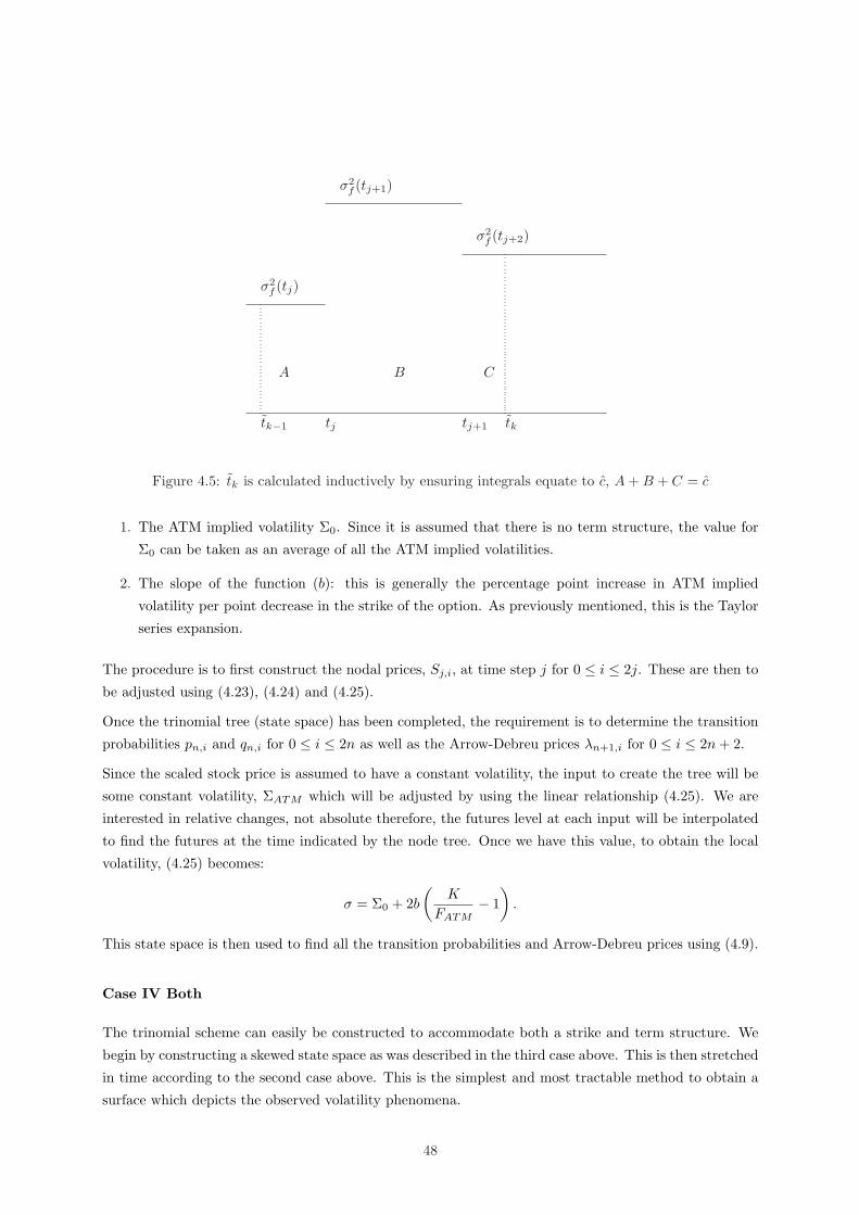
Case III: Skew Structure
We now apply the results of §4.2.2. In the case that the local volatility function is of the form σ(S), the
state space is constructed to accommodate a linear relationship between implied volatility and strike. We
assume that there is no term structure. The input requirement is
47
σ2f (tj)
σ2f (tj+1)
σ2f (tj+2)
A B C
tk−1 tj tj+1 tk
Figure 4.5: tk is calculated inductively by ensuring integrals equate to c, A + B + C = c
1. The ATM implied volatility Σ0. Since it is assumed that there is no term structure, the value for
Σ0 can be taken as an average of all the ATM implied volatilities.
2. The slope of the function (b): this is generally the percentage point increase in ATM implied
volatility per point decrease in the strike of the option. As previously mentioned, this is the Taylor
series expansion.
The procedure is to first construct the nodal prices, Sj,i, at time step j for 0 ≤ i ≤ 2j. These are then to
be adjusted using (4.23), (4.24) and (4.25).
Once the trinomial tree (state space) has been completed, the requirement is to determine the transition
probabilities pn,i and qn,i for 0 ≤ i ≤ 2n as well as the Arrow-Debreu prices λn+1,i for 0 ≤ i ≤ 2n + 2.
Since the scaled stock price is assumed to have a constant volatility, the input to create the tree will be
some constant volatility, ΣATM which will be adjusted by using the linear relationship (4.25). We are
interested in relative changes, not absolute therefore, the futures level at each input will be interpolated
to find the futures at the time indicated by the node tree. Once we have this value, to obtain the local
volatility, (4.25) becomes:
σ = Σ0 + 2b
(K
FATM− 1
).
This state space is then used to find all the transition probabilities and Arrow-Debreu prices using (4.9).
Case IV Both
The trinomial scheme can easily be constructed to accommodate both a strike and term structure. We
begin by constructing a skewed state space as was described in the third case above. This is then stretched
in time according to the second case above. This is the simplest and most tractable method to obtain a
surface which depicts the observed volatility phenomena.
48
4.6.3 Non-Constant Time Intervals and a Dividend Yield
If it is the case that the input data (option expiry times) is not equally spaced, the resulting trinomial
tree should display such a feature. The original Derman-Kani-Chriss algorithm can be altered to allow for
such a modification in the case where the option prices are calculated using Black-Scholes, not a trinomial
tree.
This is done in exactly the same manner as in Chapter 3, §3.7.1.
49
Chapter 5
Characterization of Local Volatility
and the Dynamics of the Smile
5.1 Introduction
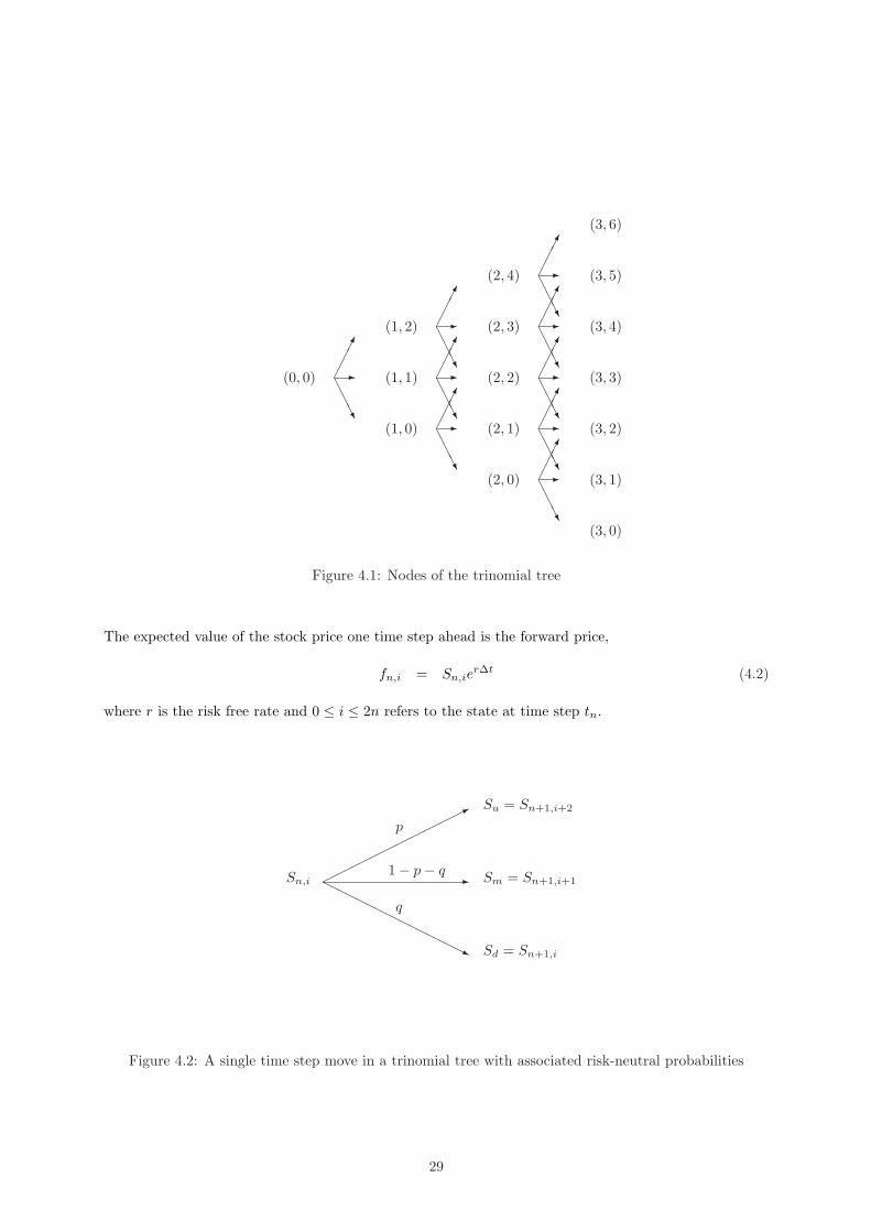
A risk-neutral diffusion process for the evolution of the underlying is proposed in (Dupire 1994):
dS
S= r(t)dt + σ(S, t)dW, (5.1)
where r(t) is the expected instantaneous stock price return and σ(S, t) is the local volatility function. W (t)
is standard Brownian motion. Here the spot follows a one dimensional diffusion process, and so the model
is complete (it allows for arbitrage pricing and hedging). Option prices can be calculated by discounting
an expectation with respect to a risk-neutral probability, under which the discounted spot has no drift,
but retains the same diffusion coefficient. In the case of European options, the expectation is taken over
terminal values of the spot, while path-dependent options are priced as discounted expected values of
the terminal payoff over all paths. Knowledge of the prices of path-dependent options is equivalent to
knowledge of the full risk-neutral diffusion, while knowing the European option prices only amounts to
knowledge of the spot distribution at the various option expiry times. The full diffusions contain more
information than the conditional laws, as distinct diffusions may generate identical conditional laws. One
attempts to choose the local volatility function σ(S, t) so as to have the model replicate the prices of
European options (for various strikes and maturities) seen trading in the market. The more maturities
we have, the closer we are to knowledge of the full risk-neutral diffusion.
5.2 Kolmogorov Equations
Before examining the local volatility function, it is necessary to derive the forward and backward Kol-
mogorov equations.
We start by developing the theory and intuition behind the backward equation. Let FWt = σ (Ws : s ≤ t)
50
be the sigma-algebra generated by Brownian motion Wt : t ≥ 0, where, s, t ≥ 0.
Let X be the unique solution that satisfies the integral equation (Bjork 2004, §5.1):
Xt = x0 +∫ t
0
µ(s,Xs)ds +∫ t
0
σ(s, Xs)dWs
subject to the existence of a constant k, such that for all x, y and t, the following hold:
The forward Kolmogorov describes the probability distribution by solving an initial-value problem, while
the backward Kolmogorov equation describes the expected final payoff by solving a final-value problem.
5.3 Relationship between Prices and Distributions
In this section, we will derive the expression for local volatility that appears in (Dupire 1994) using
the approach presented in (Derman & Kani 1994). Let φ (ST , S0, T ) denote the risk-neutral probability
density function associated with (5.1). It is defined as the probability that the stock price reaches ST
53
at time T having the initial value S0 at time 0. It satisfies both the backward and forward Kolmogorov
equations with boundary condition φ (S0, ST , 0) = δ (ST − S0), where δ(x) is the Dirac delta function.
These equations are parabolic partial differential equations. The backward equation involves derivatives
with respect to current state and time while the forward equation involves derivatives with respect to
future state and time. The backward Kolmogorov equation requires terminal conditions and is solved
for, backwards in time:
∂φ
∂T= 1 1
2σ2S2
0
∂2φ
∂S20
+ rS0∂φ
∂S0(5.8)
The forward Kolmogorov (Fokker-Planck) equation requires initial conditions and is solved for T > 0:
∂φ
∂T= 2 1
2∂2
∂S2T
(σ2S2
T φ)− r
∂
∂ST(ST φ) (5.9)
Let Z(0, t) be the discount function given by
Z(0, t) = exp(−
∫ t
0
r (s) ds
)(5.10)
Now we briefly review the main results of (Breeden & Litzenberger 1978). The collection of European
call option prices, C (S0,K, T ), with current spot S0, maturity T and of different strikes K, yields the
risk-neutral density function φ through the relationship:
C (S0,K, T ) = Z(0, T )∫ ∞
K
φ (S0, ST , T ) (ST −K) dST (5.11)
We now use the following well-known formula, the Leibnitz rule, for differentiation of a definite integral
with respect to a parameter (Abramowitz & Stegun 1974):
d
da
∫ φ(a)
ψ(a)
f (x, a) dx = f (φ (a) , a)dφ (a)
da− f (ψ (a) , a)
dψ (a)da
+∫ φ(a)
ψ(a)
d
daf (x, a) dx
1If we consider the diffusion process of (5.1), Proposition (2) can be applied. For all t < T , we have that
∂φ
∂t+Aφ = 0
∂φ
∂t+ rS0
∂φ
∂S0+ 1
2σ2S2
0
∂2φ
∂S02
= 0
⇒ rS0∂φ
∂S0+ 1
2σ2S2
0
∂2φ
∂S02
=∂φ
∂T,
where the Ito operator is defined by (5.5).2Using Proposition (3) and the definition of the adjoint Ito operator (5.7), we have that for all T > t (as the forward
equation relies on initial conditions and describes behaviour forward in time),
∂φ
∂T−A∗φ = 0
∂φ
∂T− −r
∂
∂ST(ST φ) +
1
2
∂2
∂S2T
`σ2S2
T φ´!
= 0
⇒ 1
2
∂2
∂S2T
`σ2S2
T φ´− r
∂
∂ST(ST φ) =
∂φ
∂T
54
Differentiating (5.11) once with respect to strike:
∂
∂KC (S0,K, T )
=∂
∂K
(Z(0, T ) lim
x→∞
∫ x
K
φ (S0, ST , T ) (ST −K) dST
)
= Z(0, T ) limx→∞
(φ (S0, x, T ) (x−K)
dx
dK− φ (S0,K, T ) (K −K)
dK
dK+
∫ x
K
φ (S0, ST , T ) (−1)dST
)
= −Z(0, T )∫ ∞
K
φ (S0, ST , T ) dST (5.12)
In this case, a = K, φ(a) and ψ(a) are constants, and f (x, a) = φ (S0, ST , T ) (ST −K). The first and
second term in the third line above are zero. Differentiating again with respect to strike:
∂2
∂K2C (S0,K, T )
= −Z(0, T ) limx→∞
(φ (S0, x, T )
dx
dK− φ (S0,K, T )
dK
dK+
∫ x
K
d
dK(φ (S0,K, T )) dST
)
= Z(0, T )φ (S0,K, T ) (5.13)
as in (Breeden & Litzenberger 1978). In practice, there are only a discrete set of of option prices and
the continuum is completed using interpolation. The right hand side of the above equation is an Arrow-
Debreu price: it is the price of a security that has a a payoff of δ (ST −K). It can be constructed using
butterflies3.
Multiplying (5.9) by Z(0, T ) (ST −K) and integrating with respect to ST yields
Z(0, T )∫ ∞
K
∂φ
∂T(ST −K) dST = Z(0, T )
∫ ∞
K
(12
∂2
∂S2T
(σ2S2
T φ)− r
∂
∂ST(ST φ)
)(ST −K) dST (5.14)
Consider the first term on the right hand side of (5.14). We use integration by parts:∫ ∞
a
f ′(ST )g(ST )dST = f(ST )g(ST )∣∣∣∣∞
a
−∫ ∞
a
f(ST )g′(ST )dST
We use this with f ′(ST ) = ∂2
∂S2T
(σ2S2
T φ)
and g(ST ) = (ST −K). So,
Z(0, T )∫ ∞
K
12
∂2
∂S2T
(σ2S2
T φ)(ST −K) dST
=Z(0, T )
2lim
x→∞
(∂
∂ST
(σ2S2
T φ)(ST −K)
∣∣∣∣x
K
−∫ x
K
∂
∂ST
(σ2S2
T φ)dST
)
=Z(0, T )
2lim
x→∞
(∂
∂ST
(σ2S2
T φ)
(ST −K)|xK − σ2S2T φ
∣∣xK
)
= Z(0, T )12σ2K2φ (ST ,K, T )
=12σ2K2 ∂2
∂K2C (S0,K, T ) (5.15)
3A butterfly payoff can be constructed by going long n (European) call options, strike K1, going short 2n call options,
strike K2 and going long n call options with strike K3, such that K2−K1 = 1n
= K3−K2. The infinitesimal width results
as n →∞.
55
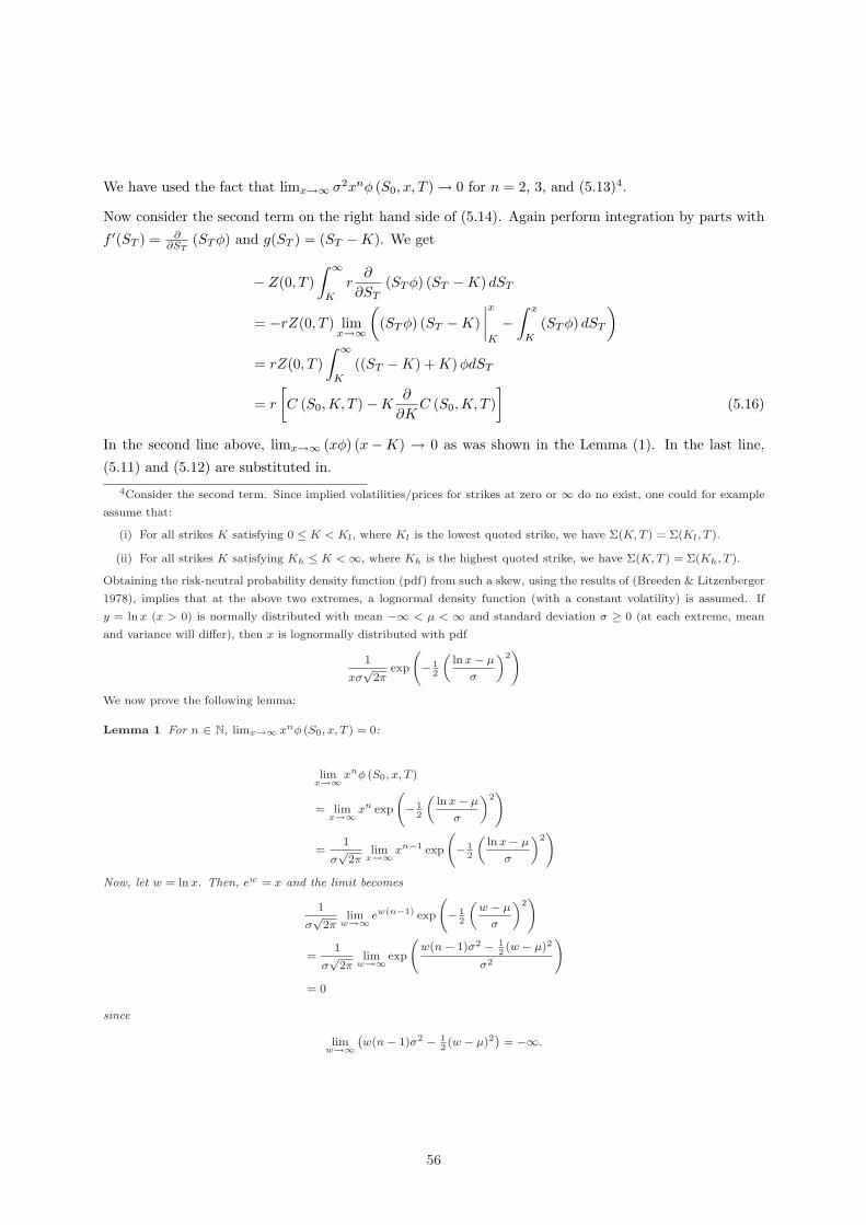
We have used the fact that limx→∞ σ2xnφ (S0, x, T ) → 0 for n = 2, 3, and (5.13)4.
Now consider the second term on the right hand side of (5.14). Again perform integration by parts with
f ′(ST ) = ∂∂ST
(ST φ) and g(ST ) = (ST −K). We get
− Z(0, T )∫ ∞
K
r∂
∂ST(ST φ) (ST −K) dST
= −rZ(0, T ) limx→∞
((ST φ) (ST −K)
∣∣∣∣x
K
−∫ x
K
(ST φ) dST
)
= rZ(0, T )∫ ∞
K
((ST −K) + K) φdST
= r
[C (S0,K, T )−K
∂
∂KC (S0,K, T )
](5.16)
In the second line above, limx→∞ (xφ) (x−K) → 0 as was shown in the Lemma (1). In the last line,
(5.11) and (5.12) are substituted in.
4Consider the second term. Since implied volatilities/prices for strikes at zero or ∞ do no exist, one could for example
assume that:
(i) For all strikes K satisfying 0 ≤ K < Kl, where Kl is the lowest quoted strike, we have Σ(K, T ) = Σ(Kl, T ).
(ii) For all strikes K satisfying Kh ≤ K < ∞, where Kh is the highest quoted strike, we have Σ(K, T ) = Σ(Kh, T ).
Obtaining the risk-neutral probability density function (pdf) from such a skew, using the results of (Breeden & Litzenberger
1978), implies that at the above two extremes, a lognormal density function (with a constant volatility) is assumed. If
y = ln x (x > 0) is normally distributed with mean −∞ < µ < ∞ and standard deviation σ ≥ 0 (at each extreme, mean
and variance will differ), then x is lognormally distributed with pdf
1
xσ√
2πexp
− 1
2
„ln x− µ
σ
«2!
We now prove the following lemma:
Lemma 1 For n ∈ N, limx→∞ xnφ (S0, x, T ) = 0:
limx→∞xnφ (S0, x, T )
= limx→∞xn exp
− 1
2
„ln x− µ
σ
«2!
=1
σ√
2πlim
x→∞xn−1 exp
− 1
2
„ln x− µ
σ
«2!
Now, let w = ln x. Then, ew = x and the limit becomes
1
σ√
2πlim
w→∞ ew(n−1) exp
− 1
2
„w − µ
σ
«2!
=1
σ√
2πlim
w→∞ exp
w(n− 1)σ2 − 1
2(w − µ)2
σ2
!
= 0
since
limw→∞
`w(n− 1)σ2 − 1
2(w − µ)2
´= −∞.
56
In order to simplify the term on the left hand side of (5.14), we note that
∂C
∂T=
∂
∂T
(Z(0, T )
∫ ∞
K
φ(ST −K)dST
)
= Z(0, T )∫ ∞
K
∂φ
∂T(ST −K) dST − rC (S0,K, T )
Therefore,
Z(0, T )∫ ∞
K
∂φ
∂T(ST −K) dST =
∂C
∂T+ rC (S0,K, T ) (5.17)
Substituting (5.15), (5.16) and (5.17) into (5.14), we get
∂C
∂T+ rC (S0,K, T ) =
12σ2K2 ∂2
∂K2C (S0,K, T ) + r
[C (S0,K, T )−K
∂
∂KC (S0,K, T )
]
Therefore,
12σ2 (K,T )K2 ∂2C
∂K2− rK
∂C
∂K− ∂C
∂T= 0
Solving for the σ (K,T )
σ (K, T ) =
√∂C∂T + rK ∂C
∂2K12K2 ∂2C
∂K2
(5.18)
which is the result proven in (Dupire 1994).
Using the following results, (5.18) can be viewed as the definition for local volatility in (5.1):
1. If (5.1) holds, then the distribution function φ (S0,K, T ) completely determines European option
prices C (S0,K, T ) for all strikes K and maturities T .
2. Conversely, call prices completely determine the distribution function using (5.13).
3. The local volatility function σ(S, t), for future stock prices S at times t, can be determined from
(5.18).
The stock price diffusion process can be entirely determined from knowledge of the stock price distribution
function.
5.4 Local Volatility in terms of Implied volatility
In this section, we will need distinguish between partial differentiation of the form
limε→0
f(x(t), t + ε)− f(x(t), t)ε
,
which we denote ∂f∂t , and partial differentiation of the form
limε→0
f(x(t + ε), t + ε)− f(x(t), t)ε
,
57
which we denote dfdt . Suppose f = f(x, t) and x = x(t). So, f is a function of t alone. Of course
df
dt=
∂f
∂t+
∂f
∂x
∂x
∂t(5.19)
This convention will be followed even if f is not a function of t alone e.g. if f = f(x, t, s), x = x(t), then
limε→0
f(x(t + ε), t + ε, s)− f(x(t), t, s)ε
will be denoted dfdt in order to distinguish from
limε→0
f(x(t), t + ε, s)− f(x(t), t, s)ε
which is ∂f∂t . Of course (5.19) holds again, even though df
dt is a function of both t and s.
(5.18) for local volatility can be extended to include a dividend yield q and is given by (Wilmott 2000,
§25.6):
σ (K, T ) =
√dCdT + (r − q) K dC
dK + qC12K2 d2C
dK2
, (5.20)
By noting that the implied volatility Σ is a function of strike and expiry i.e. Σ = Σ(K, T ), the above
partial derivatives can be obtained with respect to Σ i.e. the local volatility function can be expressed as
a function of implied volatility rather than of option prices.
as ε → 0, is a regular or straightforward perturbation expansion, with ε as perturbation parameter.
The function f(x) is a solution to an algebraic, integral or differential equation. f(x, ε) is the perturbed
solution with εjfj(x) as the jth order solution. The regular expansion is performed up to order 2 or
3 then substituted into the original equation for f(x). The solution is then obtained by equating like
powers of ε and solving for each.
If it is not possible to find an asymptotic expansion (to be defined below) for a given function, it will be
necessary to use a general sequence of functions.
Definition 3 Asymptotic Sequence
(Cole & Kevorkian 1981, §1.2) Consider a sequence of functions of ε, φn(ε) for n = 1, 2, . . .. Such a
sequence is asymptotic if
φn+1(ε) = o(φn(ε)) as ε → ε0
for each n. If the sequence is infinite and φn+1 = o(φn) uniformly in n, the sequence is said to be uniform
in n.
63
Definition 4 Asymptotic Expansion
(Cole & Kevorkian 1981, §1.2) A sum of terms of the form∑N
n=1 an(x)φn(ε) is called an asymptotic
expansion of the function f(x, ε) to N terms (N may be infinite) as ε → ε0 with respect to the sequence
φn(ε) if
f(x, ε)−M∑
n=1
an(x)φn(ε) = o(φM ) as ε → ε0
for each M = 1, 2, . . . , N . Or equivalently,
f(x, ε)−M−1∑n=1
an(x)φn(ε) = O(φM ) as ε → ε0
for each M = 2, . . . , N .
If the order relations hold uniformly in the domain, then the expansion becomes uniformly valid in the
domain. Given a function f(x, ε) and an asymptotic sequence φn(ε), each of the an(x) can be uniquely
calculated using the above definition. Thus,
a1(x) = limε→ε0
f(x, ε)φ1(ε)
a2(x) = limε→ε0
f(x, ε)− a1(x)φ1(ε)φ2(ε)
ak(x) = limε→ε0
f(x, ε)−∑k−1n=1 an(x)φn(ε)
φk(ε)
Solutions for Algebraic, Integral or Differential Equations
Let f(x, ε) be a solution to an algebraic, integral or differential equation, with x the independent variable
and ε a small parameter. If the equation cannot be solved for arbitrary ε, the solution can be represented as
an asymptotic expansion of the parameter. This is called a parameter perturbation. In the straightforward
expansion given by Definition 2, the term εn+1f(x)n+1 should be a small correction to the term εnf(x)n.
Consequently, this type of expansion breaks down when εn+1fn+1 = O(εnfn), where n = 0, 1, or 2. If
the expansion, using a finite number of terms does not represent the solution for all values of x, then the
expansion is non-uniformly valid for all x. This then leads to singular perturbation problems. These are
the rule, as opposed to the exception (regular perturbation problems).
5.5.4 Solving for Option Prices and Implied Volatility
Let V (t, f) be the date t value of a European call option, with strike K and expiry and settlement dates
tex and tset respectively. As before, F (t) is the forward price process which follows equation (5.27). Under
the forward measure we have
V (t, f) = Z(t, tset)E[(F (tex)−K)+ |F (t) = f
]. (5.30)
Let
Q(t, f) := E[(F (tex)−K)+ |F (t) = f
](5.31)
64
be the expected payoff of the option. The expectation is over the probability distribution generated by
F (t). Q(t, T ) must satisfy the backward Kolmogorov equation in §5.2:
Qt +12α2(t)A2(f)Qff = 0, t < tex, (5.32)
subject to the terminal condition
Q(tex, f) = (f −K)+. (5.33)
We begin by selecting an appropriate perturbation parameter, ε ≡ A(K) ¿ 1, and scale equations (5.32)
and (5.33) by defining
ψ := ψ(t) =∫ tex
t
α2(s)ds, (5.34)
x := x(f) =1ε(f −K), (5.35)
Q(ψ, x) =1εQ(t, f). (5.36)
Note that in Black’s model, α(t) = σB and A(K) = K. Thus it might not be the case that A(K) ¿ 1
in equity markets, while it would be in the interest rate market. This problem is easily resolved by some
normalization procedure that can be applied to A(K) with the inverse procedure applied to α(t). We will
see a similar strategy in Chapter 9.
In terms of the variables x, ψ and Q, we have
∂Q
∂t= ε
∂Q
∂ψ
∂ψ
∂t
= −ε∂Q
∂ψα2(t),
∂Q
∂f= ε
∂Q
∂x
∂x
∂f
= ε∂Q
∂x
1ε
=∂Q
∂x,
∂2Q
∂f2=
∂2Q
∂x2
1ε
For ψ > 0, (5.32) then becomes
−εQψα2(t) +12α2(t)A2(f)Qxx
1ε
= 0
⇒ Qψ − 12
A2(K + εx)A2(K)
Qxx = 0, (5.37)
since f = K + εx, and (5.33) transforms to
Q = x+, ψ = 0. (5.38)
Therefore, in terms of Q(ψ, x) the option value is given by
V (t, f) = Z(t, tset)A(K)Q(
ψ(t),f −K
A(K)
).
65
By using a Taylor expansion of A(K + εx),
A(K + εx) =∞∑
j=0
Aj(K)j!
εjxj
= A(K)∞∑
j=0
εjxj
j!Aj(K)A(K)
⇒ A(K + εx)A(K)
=∞∑
j=0
νj
j!εjxj ,
where
νj =A(j)(K)A(K)
, for j = 1, 2, . . .
All expansions will be done up to order ε2. Therefore,
A2(K + εx)A2(K)
=
∞∑
j=0
νj
j!εjxj
2
=∞∑
j=0
(νj
j!εjxj
)2
+ 2∞∑
j=0
j−1∑
k=0
νj
j!εjxj νk
k!εkxk
= 1 + ν21ε2x2 + 2ν1εx + 2
ν2
2ε2x2 (1 + ν1εx) + . . .
= 1 + 2ν1εx +(ν21 + ν2
)ε2x2 + . . .
Substituting this into (5.37):
Qψ − 12
(1 + 2ν1εx +
(ν21 + ν2
)ε2x2 + . . .
)Qxx = 0.
Therefore, for ψ > 0, up to ε2,
Qψ − 12Qxx = ν1εxQxx +
12ε2
(ν21 + ν2
)x2Qxx + . . . (5.39)
subject to
Q = x+, at ψ = 0.
In order to solve for Q, we perform a regular perturbation expansion (with ε as the expansion parameter)
according to Definition 2:
Q = 7Q0 + εQ1 + ε2Q2 + . . .
Substituting this expansion into (5.39), we get
Q0ψ −
12Q0
xx + εQ1ψ −
12εQ1
xx + ε2Q2ψ −
12ε2Q2
xx + . . .
= ν1εx(Q0
xx + εQ1xx + ε2Q2
xx + . . .)
+12ε2
(ν21 + ν2
)x2
(Q0
xx + εQ1xx + ε2Q2
xx + . . .)
= ν1εxQ0xx + ν1ε
2xQ1xx +
12ε2
(ν21 + ν2
)x2Q0
xx + . . .
Equating like powers of ε, the following hierarchy of PDEs result:7The powers of the function Q refer to the order of the solution. This notation is used here and in Chapter 9, as the use
of subscripts will be for partial differentiation.
66
1. At order 0, we have
Q0ψ −
12Q0
xx = 0, for ψ > 0
Q0 = x+ at ψ = 0, (5.40)
which is basically the heat equation.
2. At order ε, we have
Q1ψ −
12Q1
xx = ν1xQ0xx, for ψ > 0
Q1 = 0 at ψ = 0. (5.41)
3. At order ε2, we have
Q2ψ −
12Q2
xx = ν1xQ1xx +
12
(ν21 + ν2
)x2Q0
xx, for ψ > 0
Q2 = 0 at ψ = 0. (5.42)
We begin by solving for Q0. The solution can be obtained using the convolution of the heat kernel with
the initial condition. This method is used in Chapter 9 to solve a similar PDE. Here, we apply the Laplace
Transform Method.
Definition 5 (James 1999, §2.2) We define the Laplace transform of a function f(x) by the expression
Lf(x) =∫ ∞
0
e−φxf(x)dx = F (φ), (5.43)
where φ is a complex variable and e−φx is called the kernel of the transformation
Clearly, the Laplace transform of the function f(x) exists if and only if the improper integral converges
for some values of φ. To establish the sufficient conditions on f(x) to ensure the transform exists, we
define the following:
Definition 6 Exponential Order
(James 1999, §2.2.3) A function f(x) is said to be of exponential order as x → ∞ if there exists a real
number µ and positive constants M and N such that
|f(x)| < Meµx
for all x > N .
The choice of µ is not unique. Thus, let the greatest lower bound µc of the set of possible values of µ be
the abscissa of convergence of the function f(x). The following theorem provides sufficient conditions
for ensuring the existence of the Laplace transform of a function. They are not necessary conditions and
are restrictive. There exist functions with infinite discontinuities that possess Laplace transforms.
67
Theorem 2 Existence of Laplace transform
(James 1999, §2.2.3) If the function f(x) is piecewise-continuous on [0,∞] and is of exponential order,
with abscissa of convergence µc, then its Laplace transform exists, with region of convergence <(φ) > µc
in the φ domain; that is
Lf(x) =∫ ∞
0
e−φxf(x)dx := F (φ), <(φ) > µc
The inverse transform f(x) of the function F (φ), written L−1 F (φ), where F (φ) = Lf(x) can
generally be found in a table of transforms (Abramowitz & Stegun 1974, §29).
Let φ = φr + iφi be the integration variable. We begin by taking the Laplace transform of the term Q0ψ
from (5.40) with <(φ) > 0, and use integration by parts to solve it. The integration is performed with
respect to ψ.∫ ∞
0
∂Q0(ψ, x)∂ψ
e−φψdψ = limα→∞
(Q0(ψ, x)e−φψ
∣∣∣α
0+ φ
∫ α
0
Q0(ψ, x)e−φψdψ
)
= limα→∞
(Q0(ψ, x)e−(φr+iφi)ψ
∣∣∣α
0+ φ
∫ α
0
Q0(ψ, x)e−(φr+iφi)ψdψ
)
= (0− x+) + φL
Q0(ψ, x)
=
−x + φQ0(φ, x) x > 0
φQ0(φ, x) x < 0
where we have defined Q0(φ, x) = L
Q0(φ, x)
. The requirement that <(φ) > 0 ensures that limα→∞ Q0(α, x)e−φα
is zero.
Let ˜Q0xx(φ, x) denote the Laplace transform of Q0
xx. Since the differentiation is with respect to x, we
treat it as a ordinary differentiation and treat φ as a constant. Therefore, the ODE to be solved is:
d2Q0(φ, x)dx2
− 2φQ0(φ, x) =
−2x x > 0
0 x < 0
For x > 0, the solution is of the form:
Q0(φ, x) = CF + PI,
where the CF is the complimentary function and PI, the particular integral. The CF satisfies the ho-
mogenous ODE
d2Q0(φ, x)dx2
− 2φQ0(φ, x) = 0
This is a second order ODE with constant coefficients. The solution is of the form
Q0(φ, x) = A(φ)e√
2φx + B(φ)e−√
2φx
where A(φ) and B(φ) are constants of integration which are functions of φ. For the PI, choose a solution
of the form ˜Q0PI(φ, x) = ax2 + bx + c, where a, b and c are constants. Noting that d2 ˜Q0
P I(φ,x)
dx2 = 2a and
substituting this into the non-homogenous ODE, we get
2a− 2φ(ax2 + bx + c
)= −2x.
68
Equating coefficients, we get
−2φb = −2,
2a− 2φc = 0,
−2φa = 0.
Thus, ˜Q0PI(φ, x) = x
φ . Therefore,
Q0(φ, x) =x
φ+ A(φ)e
√2φx + B(φ)e−
√2φx (5.44)
In the case that x < 0, the solution is
Q0(φ, x) = C(φ)e√
2φx + D(φ)e−√
2φx (5.45)
In order to avoid solutions which grow exponentially at ±∞, we set A(φ) = D(φ) = 0. Consequently, the
solution will be bounded and unique.
To determine the function values B(φ) and C(φ), we equate Q0(φ, x) and dQ0(φ,x)dx at x = 0. This can
be interpreted as saying that the rate of change of the expected value of the payoff, with respect to the
independent variable, in both the transformed and untransformed space, is equivalent to the expected
value of the payoff at x = 0.
Q0(φ, 0) =
B(φ) x > 0
C(φ) x < 0(5.46)
dQ0(φ, x)dx
=
1φ −
√2φB(φ)e−
√2φx x > 0√
2φC(φ)e√
2φx x < 0(5.47)
(5.46) requires B(φ) = C(φ). Using this in (5.47) and setting x = 0, we get that
1φ−
√2φB(φ) =
√2φB(φ)
⇒ B(φ) =1φ
12√
2φ
=1
(2φ)3/2.
Thus, we have that
Q0(φ, x) =
xφ x > 0
0 x < 0
+
1
(2φ)3/2e−√
2φ|x|.
Using a table of Laplace transform inversion formulae (Abramowitz & Stegun 1974, §29), we have that
Q0(ψ, x) = xΦ(
x√ψ
)+
√ψ
2πe−x2/2ψ, (5.48)
where Φ (·) is the cumulative normal density function.
69
We now note two ways of generating further solutions to PDEs given an initial one. Suppose F (ψ, x) is
a previously determined solution to the PDE Fψ = 12Fxx. Firstly, differentiating F any number of times
with respect to x and/or ψ results in another solution (with a different boundary condition). Secondly,
suppose we are trying to solve the PDE:
uψ(ψ, x)− 12ux(ψ, x) = mψjF (ψ, x).
We claim u(ψ, x) = mψj+1
j+1 F (ψ, x) is a solution, of course it has initial condition u(0, x) = 0. To see this,
we calculate
uψ(ψ, x)− 12uxx(ψ, x)
=∂
∂ψ
(m
ψj+1
j + 1F (ψ, x)
)− 1
2∂2
∂x2
(m
ψj+1
j + 1F (ψ, x)
)
= m
(ψjF (ψ, x) +
ψj+1
j + 1Fψ(ψ, x)
)− m
2ψj+1
j + 1Fxx(ψ, x)
= mψjF (ψ, x). (5.49)
Let G(ψ, x) = Q0. G is a solution to the PDE (5.40); we will use the above tricks to find solutions for
Q1 and Q2. In preparation for this, we calculate some of the partial derivatives of G with respect to ψ
and x.
Using the product rule of differentiation,
Gx = Φ(
x√ψ
)+ x
1√2πψ
e−x2/2ψ − x1√2πψ
e−x2/2ψ = Φ(
x√ψ
)
Gxx =1√2πψ
e−x2/2ψ
Gψ = x
( −1√2π
e−x2/2ψ x
2ψ√
ψ
)+
12
1√2π
1√ψ
e−x2/2ψ +
√ψ
2πe−x2/2ψ x2
2ψ2
= e−x2/2ψ
( −x2
2ψ√
2πψ+
12√
2πψ+
x2
2ψ√
2πψ
)
=12
1√2πψ
e−x2/2ψ
Gψψ =−1
2√
2π
12
1ψ√
ψe−x2/2ψ +
12
1√2πψ
e−x2/2ψ x2
2ψ2
=1√2πψ
e−x2/2ψ
(x2 − ψ
4ψ2
)
Gψx =12
−x
ψ√
2πψe−x2/2ψ
Gψψψ =−1√2π
12
1ψ√
ψe−x2/2ψ
(x2 − ψ
4ψ2
)+
1√2πψ
e−x2/2ψ x2
2ψ2
(x2 − ψ
4ψ2
)+
1√2πψ
e−x2/2ψ
(−2x2
4ψ3+
14ψ2
)
=1√2πψ
e−x2/2ψ
(x2 − ψ
4ψ2
) (x2
2ψ2− 1
2ψ
)+
1√2πψ
e−x2/2ψ
(ψ − 2x2
4ψ3
)
=1√2πψ
e−x2/2ψ
(ψ2 − ψx2 + x4 − ψx2 + 2ψ2 − 4ψx2
8ψ4
)
=1√2πψ
e−x2/2ψ
(3ψ2 − 6ψx2 + x4
8ψ4
)
70
Using the partial derivatives and property (5.49), at O(ε), we are solving for Q1. For ψ > 0, we have
Q1ψ −
12Q1
xx = ν1xGxx = −2ν1ψGψx,
with Q1 = 0 at ψ = 0. Therefore,
Q1 = −2ν1ψ2
2Gψx = −ν1ψ
2Gψx
= ν1ψxGψ (5.50)
At O(ε2), we have for ψ > 0:
Q2ψ −
12Q2
xx = ν1xQ1xx +
12
(ν21 + ν2
)x2Gxx (5.51)
In order to simplify this, we begin by finding Q1xx.
Q1xx =
∂2
∂x2ν1ψxGψ
= ν1ψ∂2
∂x2
(x
12√
2πψe−x2/2ψ
)
=ν1ψ
2√
2πψ
∂2
∂x2
(xe−x2/2ψ
)
=ν1ψ
2√
2πψ
∂
∂x
(e−x2/2ψ
(1− x2
ψ
))
=ν1ψ
2√
2πψ
(e−x2/2ψ−x
ψ
(1− x2
ψ
)− e−x2/2ψ 2x
ψ
)
=ν1ψ
2√
2πψe−x2/2ψ
(x3
ψ2− x
ψ− 2x
ψ
)
=ν1ψ√2πψ
e−x2/2ψ
(x3 − 3ψx
2ψ
)
Substituting this into (5.51), we get
Q2ψ −
12Q2
xx = ν1xν1ψ√2πψ
e−x2/2ψ
(x3 − 3ψx
2ψ
)+
12
(ν21 + ν2
)x2 1√
2πψe−x2/2ψ
=1√2πψ
e−x2/2ψ
(ν21
(x4 − 3ψx2
2ψ+
x2
2
)+
ν2
2x2
)
=1√2πψ
e−x2/2ψ
(ν21
(x4 − 2ψx2
2ψ
)+
ν2
2x2
)
A suitable linear expression using the partial derivatives Gψ, Gψψ and Gψψψ is to be constructed to
equate to the coefficient of ν21 . Let 1√
2πψe−x2/2ψ ≡ C. Gψψψ is the only expression which contains a term
with x4. Since we require C x4
2ψ , we need to take the multiple 4ψ3Gψψψ. This results in
C4ψ3
(3ψ2 − 6ψx2 + x4
8ψ4
)= C
(x4
2ψ− 3x2 +
32ψ
)
The next term we require is −Cx2. Currently having −3Cx2, we add to the above expression 8ψ2Gψψ =
C(2x2 − 2ψ) which gives C(
x4
2ψ − x2 − ψ2
). The final step involves removing the term −C
2 ψ. This is
71
achieved by adding the term ψGψ = C2 ψ. Therefore, we have that
1√2πψ
e−x2/2ψν21
(x4 − 2ψx2
2ψ
)= 4ψ3Gψψψ + 8ψ2Gψψ + ψGψ (5.52)
The same procedure follows for the coefficient of ν2, C2 x2. The partial derivatives to be used will be
Gψ and Gψψ since the highest power of x in the coefficient is x2. Since we require C2 x2, begin with the
multiple 2ψ2Gψψ = C2 (x2 − ψ). To remove the term −C
2 ψ, add ψGψ = C2 ψ. Therefore,
1√2πψ
e−x2/2ψ ν2
2x2 = 2ψ2Gψψ + ψGψ (5.53)
Using property (5.49), (5.52) and (5.53) are integrated, enabling us to solve for Q2:
4ψ3Gψψψ + 8ψ2Gψψ + ψGψ = ψ4Gψψψ +83ψ3Gψψ +
ψ2
2Gψ,
2ψ2Gψψ + Gψ =23ψ3Gψψ +
12ψ2Gψ.
So, the solution Q2 is:
Q2 = ν21
(ψ4Gψψψ +
83ψ3Gψψ +
ψ2
2Gψ
)+ ν2
(23ψ3Gψψ +
12ψ2Gψ
)(5.54)
We then write this in a concise format. Looking at the coefficient of ν21 , we have that
ψ4Gψψψ +83ψ3Gψψ +
ψ2
2Gψ = ψ4C
(3ψ2 − 6ψx2 + x4
8ψ4
)+
83ψ3C
(x2 − ψ
4ψ2
)+
ψ2
212C
=(
x4
8− 3
4ψx2 +
38ψ2 +
23ψx2 − 2
3ψ2 +
14ψ2
)C
=(
x4
8− 1
12ψx2 − 1
24ψ2
)C.
Expressing the above line in terms of Gψψ and Gψ, we get that
12ψ2x2Gψψ +
112
ψx2Gψ − 112
ψ2Gψ =(
x4
8− 1
8ψx2 +
124
ψ2x2 − 124
ψ2
)C
=(
x4
8− 1
12ψx2 − 1
24ψ2
)C. (5.55)
The coefficient of ν2 is then expanded:
23ψ3Gψψ +
12ψ2Gψ =
23ψ3C
(x2 − ψ
4ψ2
)+ ψ2 C
4
=(
16ψx2 +
112
ψ2
)C.
Rewriting the above line in terms of Gψ, we get(
16ψx2 +
112
ψ2
)C =
112
(2ψx2 + ψ2
)C
=ψ
6(2x2 + ψ
)Gψ. (5.56)
72
Therefore, substituting (5.55) and (5.56) into (5.54), we have
Q2 =12ν21ψ2x2Gψψ +
112
ν21
(x2 − ψ
)ψGψ +
16ν2
(2x2 + ψ
)ψGψ. (5.57)
The solution of Q up to O(ε2) is then given by substituting (5.48), (5.50) and (5.57) into the regular
perturbation expansion:
Q = Q0 + εQ1 + ε2Q2 + . . .
= G + εν1ψxGψ +12ε2ν2
1ψ2x2Gψψ + ε2
(4ν2 + ν2
1
12x2 +
2ν2 − ν21
12ψ
)ψGψ (5.58)
Define
ψ := ψ
(1 + εν1x + ε2
(4ν2 + ν2
1
12x2 +
2ν2 − ν21
12ψ
)+ . . .
).
Then Q(ψ, x) can be re-written as Q(ψ, x) = G(ψ, x). This is true up to O(ε2). Given the definition of
ψ, we can expand G(ψ, x) around ψ:
G(ψ, x) = G(ψ, x) + ψ
(εν1x + ε2
(4ν2 + ν2
1
12x2 +
2ν2 − ν21
12ψ
)+ . . .
)Gψ(ψ, x)
+ψ2
2
(εν1x + ε2
(4ν2 + ν2
1
12x2 +
2ν2 − ν21
12ψ
)+ . . .
)2
Gψψ(ψ, x) + . . .
= G(ψ, x) + εν1ψxGψ(ψ, x) + ε2
(4ν2 + ν2
1
12x2 +
2ν2 − ν21
12ψ
)ψGψ(ψ, x) +
12ε2ν2
1ψ2x2Gψψ(ψ, x) + . . .
= Q(ψ, x)
by (5.58).
Recall the European call option value at time t is given by
V (t, f) = Z(t, tset)εQ(ψ, x) = Z(t, tset)εG(ψ, x) = 8Z(t, tset)G(ε2ψ, εx) = Z(t, tset)G(A2(K)ψ, f −K
),
which is directly from the definition of x and ε. By defining
ψ∗ := A2(K)ψ = A2(K)ψ(
1 + εν1x + ε2
(4ν2 + ν2
1
12x2 +
2ν2 − ν21
12ψ
)+ . . .
)
= A2(K)ψ(
1 + ν1 (f −K) +4ν2 + ν2
1
12(f −K)2 +
2ν2 − ν21
12A2(K)ψ + . . .
),
8By directly substituting G(ε2ψ, εx) into (5.48), we can show that εG(ψ, x) = G(ε2ψ, εx). We have that
εG(ψ, x) = ε
0B@xΦ
0B@ xq
ψ
1CA+
sψ
2πe−x2/2ψ
1CA .
Then,
G(ε2ψ, εx) = εxΦ
0B@ εxq
ψε2
1CA+
sψε2
2πe−ε2x2/2ψε2
= εxΦ
0B@ xq
ψ
1CA+ ε
sψ
2πe−x2/2ψ .
73
we find the option value is given by
V (t, f) = Z(t, tset)G (ψ∗, f −K) . (5.59)
To obtain the equivalent Black implied volatility, we take f −K to be O(ε) and A2(K)ψ as O(ε2) and
use the Maclaurin expansion for small x of√
1 + x = 1 + 12x− 1
8x2 + . . .. Up to order ε2,
√ψ∗ = A(K)
√ψ
(1 +
12ν1 (f −K) +
4ν2 + ν21
24(f −K)2 +
2ν2 − ν21
24A2(K)ψ − 1
8ν21(f −K)2 + . . .
)
= A(K)√
ψ
(1 +
12ν1 (f −K) +
2ν2 − ν21
12(f −K)2 +
2ν2 − ν21
24A2(K)ψ + . . .
). (5.60)
Given that ν1 = A′(K)A(K) , the first two terms of the expansion for
√ψ∗ are
A(K)√
ψ + A(K)√
ψ12
A′(K)A(K)
(f −K) =√
ψ
(A(K) +
12A′(K) (f −K)
). (5.61)
Define fav := 12 (f + K). By noting that K = fav − 1
2 (f −K), we can expand A around fav:
A(K) = A(fav − 1
2 (f −K))
= A(fav)− 12(f −K)A′(fav) +
12
(f −K)2
4A′′(fav) + . . .
A′(K) = A′(fav)− 12(f −K)A′′(fav) +
12
(f −K)2
4A′′′(fav) + . . .
Then, substituting this into the right hand side of (5.61), we get
√ψ
(A(K) +
12A′(K) (f −K)
)
=√
ψ
(A(fav)− 1
2(f −K)A′(fav) +
18(f −K)2A′′(fav)
+12
(f −K)(
A′(fav)− 12(f −K)A′′(fav) +
18(f −K)2A′′′(fav)
)+ . . .
)
=√
ψA(fav)(
1− 18
(f −K)2A′′(fav)A(fav)
)+ O(ε3)
=√
ψA(fav)(
1− 18γ2 (f −K)2
)+ O(ε3)
where, for k = 1, 2, . . .,
γk =A(k)(fav)A(fav)
.
Since we are expanding to O(ε2
), the νk in the last two terms of (5.60) can be changed to γk without
affecting the computation since they are O(ε2
)and are both multiplied by A(fav)
√ψ which is O (ε). 9
9By noting that K = fav − 12(f −K), we expand the following:
A(K) = A(fav)− 1
2(f −K)A′(fav) +
1
8(f −K)2A′′(fav) + . . .
A′(K) = A′(fav)− 1
2(f −K)A′′(fav) +
1
8(f −K)2A′′′(fav) + . . .
A′′(K) = A′′(fav)− 1
2(f −K)A′′′(fav) +
1
8(f −K)2A′′′′(fav) + . . .
74
Upon substitution into (5.60),
√ψ∗ = A(fav)
√ψ
(1− 1
8γ2 (f −K)2 +
2γ2 − γ21
12(f −K)2 +
2γ2 − γ21
24A2(fav)ψ + . . .
)
= A(fav)√
ψ
(1 +
γ2 − 2γ21
24(f −K)2 +
2γ2 − γ21
24A2(fav)ψ + . . .
)(5.62)
In order to obtain the implied volatility, it is necessary to consider the special case where we start with
Black’s model: dF (t) = σBF (t)dW ; so α(t) = σB and A(F ) = F . The value of the option price V (t, f)
is then given by
V (t, f) = Z(t, tset)G (ψB , f −K) ,
where√
ψB is obtained by substituting σB and F into the expression for√
ψ∗, (5.62). We have that
Looking at the remaining four terms of (5.60), we use the above expansions to verify that the substitution of γk in place of
νk can be done using the fact that (f −K)2 and A2(fav) are O(ε2), and A(fav) is O(ε):
1.
1
6A(K)
pψν2(f −K)2 =
√ψ
6A′′(K)(f −K)2
=
√ψ
6
„A′′(fav)− 1
2(f −K)A′′′(fav) +
1
8(f −K)2A′′′′(fav) + . . .
«(f −K)2
= O(ε3)
2.
−1
12A(K)
pψν2
2 (f −K)2 =−√ψ
12
(A′(K))2
A(K)(f −K)2
=−√ψ
12
„A′′(fav)− 1
2(f −K)A′′′(fav) +
1
8(f −K)2A′′′′(fav) + . . .
«2
·„
A(fav)− 1
2(f −K)A′(fav) +
1
8(f −K)2A′′(fav) + . . .
«−1
(f −K)2
=−√ψ
12
“`A′′(fav)
´2+ . . .
”„A(fav) +
1
2(f −K)A′(fav) + . . .
«(f −K)2
= O(ε3)
3.
1
12A3(K)ψ3/2ν2 =
ψ3/2
12A2(K)A′′(K)
=ψ3/2
12
„A(fav)− 1
2(f −K)A′(fav) +
1
8(f −K)2A′′(fav) + . . .
«2
·„
A′′(fav)− 1
2(f −K)A′′′(fav) +
1
8(f −K)2A′′′′(fav) + . . .
«
= O(ε3)
4.
−1
24A3(K)ψ3/2ν2
1 =−ψ3/2
24A(K)A′(K)
=−ψ3/2
24
„A(fav)− 1
2(f −K)A′(fav) +
1
8(f −K)2A′′(fav) + . . .
«·
„A′(fav)− 1
2(f −K)A′′(fav) +
1
8(f −K)2A′′′(fav) + . . .
«
= O(ε3)
75
A(fav) = fav and√
ψ = σB
√tex − t. We also note that γ1 = 1
favand γk = 0 for all k > 1. This yields
√ψB = favσB
√tex − t
(1− (f −K)2
12f2av
− σ2B (tex − t)
24+ . . .
)
Since G (ψB , f −K) is an increasing function of ψB , the Black price will coincide with the correct price
if and only if√
ψB =√
ψ∗.
Doing this yields the expression for implied volatility:
favσB
√tex − t
(1− (f −K)2
12f2av
− σ2B (tex − t)
24+ . . .
)
= A(fav)√
ψ
(1 +
γ2 − 2γ21
24(f −K)2 +
2γ2 − γ21
24A2(fav)ψ + . . .
). (5.63)
Now (1− (f −K)2
12f2av
− σ2B (tex − t)
24+ . . .
) (1 +
(f −K)2
12f2av
+σ2
B (tex − t)24
)= 1 + O(ε3)
(It is a difference of squares.) Hence, by multiplying both sides of (5.63) by(
1 +(f −K)2
12f2av
+σ2
B (tex − t)24
),
and dividing by fav
√tex − t, we get
σB
=√
ψ√tex − t
A(fav)fav
[1 +
γ2 − 2γ21
24(f −K)2 +
2γ2 − γ21
24A2(fav)ψ + . . .
][1 +
(f −K)2
12f2av
+σ2
B (tex − t)24
+ . . .
]
=√
ψ√tex − t
A(fav)fav
[1 +
(γ2 − 2γ2
1 +2
f2av
)(f −K)2
24+
2γ2 − γ21
24A2(fav)ψ +
σ2B (tex − t)
24+ . . .
].
As a separate calculation, note that
σB =√
ψ√tex − t
A(fav)fav
[1 +
(γ2 − 2γ2
1 +2
f2av
)(f −K)2
24+
2γ2 − γ21
24A2(fav)ψ +
σ2B (tex − t)
24+ . . .
]
=√
ψ√tex − t
A(fav)fav
[1 + O(ε2)].
So squaring both sides we get
σ2B =
ψ
tex − t
A2(fav)f2
av
[1 + O(ε2)],
so
σ2B(tex − t) =ψ
A2(fav)f2
av
[1 + O(ε2)]
=ψA2(fav)
f2av
+ O(ε4)
76
since ψA2(fav)
f2av
is itself O(ε2). Now, returning to the expression for σB , we have at time t = 0, f = f0
σB
=√
ψ√tex − t
A(fav)fav
[1 +
(γ2 − 2γ2
1 +2
f2av
)(f −K)2
24+
(2γ2 − γ2
1 +1
f2av
)A2(fav)ψ
24+ . . .
]
= aA(fav)
fav
[1 +
(γ2 − 2γ2
1 +2
f2av
)(f −K)2
24+
(2γ2 − γ2
1 +1
f2av
)a2A2(fav)(tex − t)
24+ . . .
], (5.64)
where
a2 =1
tex − tψ
=1
tex − t
∫ tex
t
α2(s)ds (5.65)
The equivalent implied volatility is given by (5.64), and is then used in Black’s formula to price call
and put options. Although the formula is not exact, (Hagan & Woodward 1998) suggest its accuracy is
comparable to that of a tree or PDE approach.
5.5.5 Incorrect Local Volatility Dynamics
Since we are trying to establish the dynamics of local volatility models, we consider the SDE, equation
(2.7) in (Hagan et al. 2002):
dF = σloc(F )FdW, F (0) = f0. (5.66)
Here, σloc(F ) is the local volatility which is a function of the forward price only. Black’s implied volatility,
as a function of strike K and the t = 0 forward price f0, is then given by equation (2.8) in (Hagan
et al. 2002):
σB(K, f0) = 10σloc (fav)(
1 +124
σ′′loc (fav)σloc (fav)
(f0 −K)2 + . . .
).
Let f0 be the t = 0 forward price and the implied volatility for a given strike K be σ0B(K). To first order,
σ0B(K) = σloc
(12 (f0 + K)
)
By translating K = 2F − f0, we have that
σ0B(2K − f0) = σloc(K).
10Given (5.66) to describe the dynamics of the forward price, it is clear that in (5.27), α(t) = 1 (therefore a = 1) and
A(fav) = σloc(fav)fav. So, substituting theses values into (5.64), we get
σB(K, f) = 1 · σloc (fav) fav
fav
„1 +
1
24
σ′′loc (fav)
σloc (fav)(f −K)2 + . . .
«
= σloc (fav)
„1 +
1
24
σ′′loc (fav)
σloc (fav)(f −K)2 + . . .
«.
77
Suppose the underlying forward value moves from f0 at time t = 0 to f1 at time t = 1,
σ0loc(K) = σ0
B(2K − f0) = 11σ1loc(K),
where σ0loc(K) and σ1
loc(K) represents the local volatilities at times t = 0 and t = 1, as a function of the
strike K, respectively. Then for an option with strike X, the implied volatility predicted by the model
at time t = 0 is given by:
σ1loc(K) = σ1
B(2K − f1)
⇒ σ0B(2K − f0) = σ1
B(2K − f1),
⇒ σ0B(X + f1 − f0) = σ1
B(X + f1 − f0) = σ1B(X).
So if f has moved left/right by f1 − f0, then σB moves to the right/left. This is contrary to known
observations and so shows that local volatility models are severely compromised.
Therefore, the dynamics are incorrect. A consequence of this is that the delta hedge value, ∆, will also
be incorrect. Consider Black’s formula for a European call option:
Vcall(0, f0) = 12Z(0, tset) (f0Φ(d1)−KΦ(d2))
= BS(f0,K, σB(f0,K), tex).
Then,
∆ :=∂Vcall
∂f0=
∂BS
∂f0+
∂BS
∂σB
∂σB
∂f0.
The second term is the local volatility model’s correction to the delta risk which is Black’s vega risk
multiplied by ∂σB
∂f0. Since the predicted dynamics are in the opposite direction to what is observed, we
can conclude that the sign of this term should be opposite to that calculated. (Hagan et al. 2002) asserts
that the Black model yields more accurate hedges than local volatility models.
11The local volatility, being state but not time dependent, is the same for each strike K at t = 0 and t = 1.12In international markets, options on futures are not fully margined and hence, the buyer will pay a premium upfront.
Consequently, the pricing formula is the Standard Black (Black 1976) formula for vanilla options. In South Africa, options
are fully margined (no premium upfront) and the pricing formula differs in that there is no discount function. i.e. the price
of call and put options are in (West 2005b, Chapter 10):
Vcall = f0Φ(d1)−KΦ(d2) ,
Vput = KΦ(−d2)− f0Φ(−d1) ,
d1,2 =ln f0
K± σ2ψex
σ√
ψex,
where the current futures level is f0, the strike K, the volatility is σ and time to maturity, ψex = tex − t. Options are
American, but there are no profitable early exercise opportunities.
78
Chapter 6
Stochastic Volatility Models
6.1 Introduction
In the preceding chapters, the focus was on deterministic, non-parametric models that enabled the local
volatility to be determined. Local volatility is, at a future market level and time, (within each model)
the volatility the index must have to ensure current market prices are fair. These models enable the
determination of Arrow-Debreu prices, which are required for the pricing and hedging of path-dependent
or exotic options. However, the models provide results that are contrary to observed phenomena. This
then leads to portfolios that do not contain the correct hedges, and mispricing of options. This will be
discussed in greater detail in Chapter 9.
Another approach to the determination of the future volatility, is rather that of stochastic volatility
(parametric) models.
In the classical Black-Scholes framework, the first fundamental theorem of mathematical finance states
that the pricing model is arbitrage free if and only if there exists an equivalent martingale measure
(EMM) (Bjork 2004, §10.9). Under this measure, the traded assets, normalized by the numeraire (risk-
free asset in general), are martingales. Furthermore, if the market model is complete (every contingent
claim is attainable), the second fundamental theorem provides the result that the EMM will be unique.
Alternatively viewed, every contingent claim can be perfectly hedged with the traded asset and risk-free
asset alone. In an arbitrage-free complete market, the prices of contingent claims can be given as their
discounted expected values under the unique EMM. This means that the discounted value of a contingent
claim is given by the initial cost of setting up the replicating strategy and the gains from trading. It
is assumed that all trading strategies are self-financing and admissible (i.e. the value of the replicating
portfolio is bounded below by zero). The martingale representation theorem is required when constructing
this portfolio.
Finding the EMM can be interpreted as applying Girsanov’s theorem and defining a martingale (Radon-
Nokodym) process, often referred to as the stochastic Doleans exponential (Bingham & Kiesel 2004,
§5.10.3), that changes the drift of the discounted stock price process to zero. So, under the EMM, it
79
becomes a martingale and through Ito’s Lemma, any sufficiently smooth function of this process (price
process of the simple contingent claim) will also be a martingale. Using this result, the Feynman-Kac
theorem is then applied to this function to obtain the above-mentioned result, the arbitrage-free price of
the claim.
Stochastic volatility models are generally two-factor models where the volatility, as well as the stock
price, are modelled using diffusion processes driven by Brownian motion(s). Since an additional source
of randomness is added to the model, without volatility being a traded asset, the market model be-
comes incomplete. The introduction of variance swaps into the market will complete the market (Hagan
et al. 2002). Incompleteness translates into non-uniqueness of the EMM. Consequently, when Girsanov’s
theorem is applied, there is no unique function (market price of volatility risk, λ), that will ensure the
uniqueness of the EMM. There are a number of different measures which can been used. Each corresponds
to different choices for λ. In general, one can choose to maximize utility or minimize risk. In complete
markets, all derivatives dependent on the underlying process will have the same value for λ. Thus, the
market determines the value for λ. If λ = 0, then the market is said to be risk-neutral. This corresponds
to the Minimal Martingale measure. The determination of this parameter is a calibration issue to be
dealt with in subsequent chapters.
Another consequence of incomplete markets is that a perfect hedge cannot be created with traded asset
and risk-free asset alone. Some common processes for the volatility, denoted σt = f(Yt) are:
in order of i = 2, . . . , d. In our case, p = 2 and the VBA algorithm to generate such a sequence can be
found in (Jackson & Staunton 2001, §12.3). To construct the columns of each of the matrices, we use the
algorithm presented by (Dias 2004) to randomly permute the original sequence.
In order to obtain Φ(0, 1) numbers without damaging the low-discrepancy properties (uniformity and
order), we will use Moro’s inversion formula presented in (Moro February 1995). Moro presented an algo-
rithm that used the (Beasley & Springer 1977) algorithm for the central part of the Normal distribution
and modelled the tails using truncated Chebyschev series. It divides the domain for u ∼ U [0, 1] into two
regions:
1. The central region of the distribution, 0.08 < u ≤ 0.92, is modelled as in Beasley and Springer;
2. The tails of the distribution, u ≤ 0.08 or u > 0.92, are modelled with Chebyschev series.
The tail performance is important for out-the-money option problems since the option’s exercise occurs
at the more extreme values, emphasizing the weight of the tail towards the option’s value.
99
Chapter 8
The Heston Model
8.1 Introduction
The two-factor model proposed in (Heston 1993) uses a solution technique based on Fourier transforms
(characteristic functions). It allows for arbitrary correlation between the volatility and the returns process.
The volatility follows an Ornstein-Uhlenbeck (OU) process. We will briefly review this process before
proceeding.
8.2 The Mean Reverting Ornstein-Uhlenbeck Process
The mean reverting OU process is an Ito process with a a linear pull-back term in the drift. It is defined
as a solution to
dYt = α (m− Yt) dt + βdZt (8.1)
where (Zt)t≥0 is a Brownian motion, α is the rate of mean reversion and m is the long-run mean of Y .
To obtain a solution to this, first consider eαtYt. Taking the differential,
d(eαtYt
)= αeαtYt + eαtdYt,
Therefore,
eαtdYt = d(eαtYt
)− αeαtYt (8.2)
Multiplying both sides of (8.1) by eαt, we get
eαtdYt = eαtα (m− Yt) dt + eαtβdZt (8.3)
Together with (8.2) implies
d(eαtYt
)= αmeαtdt + eαtβdZt
100
Solving for this given that Y0 = y:
eαtYt = y +∫ t
0
αmeαsds +∫ t
0
βeαsdZs
⇒ Yt = e−αty +∫ t
0
αme−α(t−s)ds +∫ t
0
βe−α(t−s)dZs
= e−αty + m(1− e−αt
)+
∫ t
0
βe−α(t−s)dZs
= m + e−αt (y −m) +∫ t
0
βe−α(t−s)dZs
To consider the distributional properties, it is clear that the integral∫ t
0βe−α(t−s)dZs has mean zero and
variance E[(∫ t
0βe−α(t−s)dZs
)2]. By the Ito Isometry (Oksendal 2004, §3.1.5),
E
[(∫ t
0
βe−α(t−s)dZs
)2]
=∫ t
0
(βe−α(t−s)
)2
ds =∫ t
0
e−2α(t−s)β2ds =β2
2α
(1− e−2αt
).
Hence, Yt ∼ N(m + e−αt (y −m) , β2
2α
(1− e−2αt
)).
8.3 Stochastic Volatility Model
The following SDEs are assumed to model the processes of spot asset St and the volatility√
Vt:
dSt = µSdt +√
VtSdW 1t (8.4)
d√
Vt = −β√
Vtdt + δdW 2t (8.5)
dW 1t dW 1
t = ρdt (8.6)
Using Ito’s Lemma, let g(t, x) = x2 to determine the process followed by the variance, Vt.
gt = 0,
gx = 2x,
gxx = 2
So,
dg(t, x) = gtdt + gxdX +12gxx(dX)2
⇒ dVt = 2√
Vt
(−β
√Vtdt + δdW 2
t
)+ δ2dt
= −2βVtdt + 2δ√
VtdW 2t + δ2dt
=(δ2 − 2βVt
)dt + 2δ
√VtdW 2
t
Rewriting this as a square-root process:
dVt = κ (θ − Vt) dt + σ√
VtdW 2t (8.7)
101
Assume a constant interest rate r. Therefore, the price at time t of a discount bond that mature at time
t + τ is given by
Z(t, t + τ) = e−rτ
As standard arbitrage arguments have already shown in Chapter 6, the value of any contingent claim
P (S, V, t) must satisfy the following PDE:
∂P
∂t+
12V S2 ∂2P
∂S2+ ρσSV
∂2P
∂S∂V+
12σ2V
∂2P
∂V 2+ r
(S
∂P
∂S− P
)
+(κ (θ − V )− λ(S, V, t)
) ∂P
∂V= 0
As before, λ(S, V, t) is the market price of volatility risk which is independent of the particular contingent
claim. This parameter can be obtained from an existing price and used to price all other claims. The
model selects a functional form of λ(S, V, t) = λV . So, the PDE a European call option, C(S, V, t), with
strike K and maturity T satisfies is:
∂C
∂t+
12V S2 ∂2C
∂S2+ ρσSV
∂2C
∂S∂V+
12σ2V
∂2C
∂V 2+ r
(S
∂C
∂S− C
)
+(κ (θ − V )− λV
) ∂C
∂V= 0 (8.8)
subject to the following boundary conditions:
C(S, V, T ) = (ST −K)+,
C(0, V, T ) = 0,
∂C
∂S(∞, V, t) = 1,
rS∂C
∂S(S, 0, t) + κθ
∂C
∂V(S, 0, t)− rC(S, 0, t) +
∂C
∂t(S, 0, t) = 0,
C(S,∞, t) = S.
By analogy with Black-Scholes, a solution of the form
C(S, V, t) = SP 1 − Z(t, T )KP 2 (8.9)
is proposed. The first term is the present value of the spot upon optimal exercise and the second term is
the present value of the strike payment. Both P 1 and P 2 must satisfy (8.8). Let x = ln S. Then, as has
been previously shown:
dxt =(µ− V
2
)dt +
√V dW 1
t (8.10)
(8.8) can be rewritten in terms of x as:
∂C
∂t+
12V
∂2C
∂x2+ ρσV
∂2C
∂x∂V+
12σ2V
∂2C
∂V 2+
(r − V
2
) ∂C
∂x− rC
+(κ (θ − V )− λV
) ∂C
∂V= 0 (8.11)
102
and the solution (8.9) becomes
C(x, V, t) = exP 1 − Z(t, T )KP 2 (8.12)
Finding all the required partial derivatives of C(x, V, t):
Cx = ex(P 1 + P 1
x
)− ZKP 2x ,
Cxx = ex(P 1 + 2P 1
x + P 1xx
)− ZKP 2xx,
CV = exP 1V − ZKP 2
V ,
CV V = exP 1V V − ZKP 2
V V ,
CV x = ex(P 1
V + P 1V x
)− ZKP 2V x,
Ct = exP 1t − ZKP 2
t − rZKP 2
where Z = Z(t, T ) = e−r(T−t).
Substituting into (8.11 ), we get
exP 1t − ZKP 2
t − rZKP 2 +12V
(ex
(P 1 + 2P 1
x + P 1xx
)− ZKP 2xx
)
+ρσV(ex
(P 1
V + P 1V x
)− ZKP 2V x
)+
12σ2V
(exP 1
V V − ZKP 2V V
)
+(r − V
2
) (ex
(P 1 + P 1
x
)− ZKP 2x
)− r(exP 1 − ZKP 2
)
+(κ (θ − V )− λV
) (exP 1
V − ZKP 2V
)= 0
Gathering terms in P 1 and P 2:
ex
[P 1
t +(r + V
2
)P 1
x +(κθ −
(κ + λ− ρσ
)V
)P 1
V +12V P 1
xx + ρσV P 1V x +
12σ2V P 1
V V
]
−ZK
[P 2
t +(r − V
2
)P 2
x +(κ (θ − V )− λV
)P 2
V +12V P 2
xx + ρσV P 2V x +
12σ2V P 2
V V
]= 0
So, the proposed solutions, P 1 and P 2 must satisfy the PDEs:
12V
∂2P j
∂x2+ ρσV
∂2P j
∂x∂V+
12σ2V
∂2P j
∂V 2+ (r + ujV )
∂P j
∂x
+(a− bjV )∂P j
∂V+
∂P j
∂t= 0, (8.13)
for j = 1, 2, where u1 = 12 , u2 = − 1
2 , a = κθ, b1 = κ + λ − ρσ and b2 = κ + λ, subject to the terminal
condition:
P j (x, V, T ) = 1x≥ln K. (8.14)
Thus, for 0 < t < T
P j(x, V, t) = EQt [1 |x ≥ lnK ] . (8.15)
The above PDE (8.13) is the Fokker-Plank equation (Kolmogorov forward equation). Equation (8.14)
can be seen as the conditional probability that the option expires in the money.
103
8.4 Solution Technique: Fourier Transform
Define the Fourier Transform and inverse transform of a function f(x), respectively as follows (James
1999):
Definition 9
F f(x) =∫ ∞
−∞f(x)e−iφxdx = F (φ) (8.16)
F−1 F (φ) =12π
∫ ∞
−∞F (φ)eiφxdφ = f(x) (8.17)
where f(x) is absolutely integrable for all t ∈ R and has at most a finite number of maxima and minima,
and a finite number of discontinuities in any finite interval, i =√−1 and φ is the transform variable.1 In
the following analysis, it is assumed that the Fourier transform variable φ = φr + iφi, where φr and φi
are real, is complex in nature. This is done to ensure the existence of the transformation of the payoff
function. In this instance, the generalized Fourier inversion formula is required:
F−1 F (φ) =12π
∫ iφi+∞
iφi−∞F (φ)eiφxdφ (8.18)
In typical option payoffs, the Fourier transform of the payoff will only exist if φi is restricted to a strip of
regularity, α < φi < β. Since the payoff depends only on the underlying, a one-dimensional transform is
required which will enable the two-dimensional PDE to be solved by means of one-dimensional integration.
8.4.1 The Direct Application of the Fourier Technique:
Standard Black-Scholes Model
To gain insight into the effectiveness of the Fourier transform and inversion formulae, a brief outline of
the process will be described below. This facilitates the reasoning behind application of such a technique.
We will consider the standard Black-Scholes pricing model, where the underlying S follows the log-normal
diffusion process with constant volatility σ and risk free rate r. Let the log-price process be represented
by x. So,
dS = rSdt + σSdZ
⇒ dx =(r − σ2
2
)dt + σdZ
1This definition may vary in terms of:
1. The signs of the exponential being reversed. i.e.
F f(x) =
Z ∞
−∞f(x)eiφxdx = F (φ), F−1 F (φ) =
1
2π
Z ∞
−∞F (φ)e−iφxdφ = f(x)
2. The constant 12π
may be split symmetrically as 1√2π
in front of (8.16) and (8.17):
F f(x) =1√2π
Z ∞
−∞f(x)e±iφxdx = F (φ), F−1 F (φ) =
1√2π
Z ∞
−∞F (φ)e∓iφxdφ = f(x)
104
The pricing function of a standard European call option on the underlying, C(x, t), is a solution to the
Black-Scholes PDE with boundary condition:
Ct +(r − σ2
2
)Cx + σ2
2 Cxx − rC = 0 (8.19)
C(x, T ) = (exT −K)+ (8.20)
Here, 0 ≤ t ≤ T , T being the expiry and K, the strike.
Since the payoff depends only on the underlying, a one-dimensional transform is required. Using a
variation of Definition (9), the transform and inverse transform of the pricing function are:
C(φ, t) =∫ ∞
−∞eiφxC(x, t)dx (8.21)
C(x, t) =12π
∫ ∞
−∞e−iφxC(φ, t)dφ (8.22)
Substituting (8.22) into (8.19), we get
12π
∫ ∞
−∞e−iφx
(Ct +
(r − σ2
2
)Cx + σ2
2 Cxx − rC)
dφ = 0
⇒ Ct +(r − σ2
2
)Cx + σ2
2 Cxx − rC = 0 (8.23)
In the above PDE, the notation Cx = ∂C∂x , refers to the Fourier transform of the partial derivative. The
requirement is to evaluate the Fourier transform of the partial derivatives: Cx, Cxx. Since the Fourier
transform is performed in the variable x for fixed t, the transform of the partial derivative in t will remain
a partial derivative in t (more precisely, the Fourier transform of ∂C∂t , ∂C
∂t is ∂ eC∂t ).
Using integration by parts and recalling that φ = φr + iφi,∫ ∞
−∞eiφx ∂C
∂xdx = lim
α→∞eiφxC(x, t)
∣∣α−α
+ iφ
∫ ∞
∞eiφxC(x, t)dx
= limα→∞
ei(φr+iφi)xC(x, t)∣∣∣α
−α+ iφ
∫ ∞
∞eiφxC(x, t)dx
= limα→∞
eiφrxe−φixC(x, t)∣∣α−α
+ iφ
∫ ∞
∞eiφxC(x, t)dx
= iφC
In the above limit, as x → ±∞, the term eiφrx behaves as an oscillating constant. For the limit to exist,
we require φi > 0 (this proves to be consistent with the required strip of regularity of the option payoff
to be demonstrated below). We also have that the option price, C(x, t), tends to zero when the asset’s
price tends to zero (or the logarithm of the asset’s price tends to −∞) and C(x, t) tends to the asset’s
price when this tends to ∞ (or the logarithm of the asset’s price tends to ∞). Consequently, the limit
goes to zero.
For the second transform, using integration by parts and the fact that ∂C∂x tends to ∞ when the asset’s
105
price tends to ∞ and zero when the asset’s price tends to zero:∫ ∞
−∞eiφx ∂2C
∂x2dx = lim
α→∞eiφx ∂C
∂x
∣∣∣∣α
−α
+ iφ
∫ ∞
−∞eiφx ∂C
∂xdx
= (iφ)2C
= −φ2C
The above limit tends to zero for the same reasons as in the first case. We require φi > 0.
We now substitute the above two transformations into (8.23) and get
Ct +[(
r − σ2
2
)iφ− σ2
2 φ2 − r]C = 0
The above equation is an ODE (variable separable) in t for every fixed φ. Thus,
dC
dt=
[r −
(r − σ2
2
)iφ + σ2
2 φ2]C
Solving this
dC
C=
[r −
(r − σ2
2
)iφ + σ2
2 φ2]dt
⇒ C(φ, t) = C(φ, T ) exp[(−r +
(r − σ2
2
)iφ− σ2
2 φ2)
(T − t)]
where C(φ, t) and C(φ, T ) is the Fourier transform of the option price and payoff respectively. First
finding C(φ, T ) and recalling that φ = φr + iφi:
C(φ, T ) =∫ ∞
−∞eiφx(ex −K)+dx
=∫ ∞
ln K
eiφxexdx−K
∫ ∞
ln K
eiφxdx
=1
1 + iφlim
α→∞ex(1+iφ)
∣∣∣α
ln K− K
iφlim
α→∞eiφx
∣∣αln K
The upper limit above does not exist unless φi > 1 in the first case and unless φi > 0 in the second.
Applying this restriction (φi > 1),
C(φ, T ) =1
1 + iφ
(0−K1+iφ
)− K
iφ
(0−Kiφ
)
=−iφK1+iφ + K1+iφ + iφK1+iφ
iφ (1 + iφ)
= − K1+iφ
φ2 − iφ(8.24)
The final step is to invert C(φ, t), the option price time t. We require the generalized Fourier transform
since φ is complex with φi > 1:
C(x, t) =12π
∫ iφi+∞
iφi−∞e−iφxC(φ, T ) exp
[(−r +
(r − σ2
2
)iφ− σ2
2 φ2)
(T − t)]dφ
=e−r(T−t)
2π
∫ iφi+∞
iφi−∞− K1+iφ
φ2 − iφexp
[−iφx +
(r − σ2
2
)iφ (T − t)− σ2
2 φ2 (T − t)]dφ
106
Simplifying the transformed payoff using partial fractions, for a and b constants, we get
−K1+iφ
φ(φ− i)= K1+iφ
[a
φ+
b
φ− i
]
−1 = (a + b) φ− ia
⇒ a = −1,
and b = i
Therefore,
C(x, t) =Ke−r(T−t)
2π
∫ iφi+∞
iφi−∞
iKiφ
φ− iexp
[−iφx +
(r − σ2
2
)iφ (T − t)− σ2
2 φ2 (T − t)]dφ
− Ke−r(T−t)
2π
∫ iφi+∞
iφi−∞
iKiφ
φexp
[−iφx +
(r − σ2
2
)iφ (T − t)− σ2
2 φ2 (T − t)]dφ
=Ke−r(T−t)
2π(<(I1) + <(I2))
The remainder of the calculation involves calculating the real part of the integrals as shown above. A
contour integral is required. The solution to the stochastic volatility model will be provided in detail in
section (8.4.3). The following pricing definition and theorems summarize the above results for general
pricing procedures.
Definition 10 (Grimmet & Stirzaker 2001) The characteristic function of X is the function φ : R −→ Cdefined by
ψ(φ) = E[eiφX
], i =
√−1
So, given the risk-neutral density and distribution function pT (x) and PT (x) respectively, of the diffusion
process x(T ), we have
ψT (φ) =∫ ∞
−∞eiφxdPT (x)
=∫ ∞
−∞eiφxpT (x)dx
The characteristic function always exists and the defining integral converges absolutely. It is also uniformly
continuous in φ. From the above definition, ψ(φ), it can be seen that ψ(φ) and ψ(−φ) are conjugate
quantities (Kendall 1945, §4.3):
<(ψ(φ)) =12
(ψ(φ) + ψ(−φ)) (8.25)
=(ψ(φ)) =12i
(ψ(φ)− ψ(−φ)) (8.26)
Another interesting result is given by the Inversion Theorem:
PT (x)− PT (0) =12π
∫ ∞
−∞ψT (φ)
1− e−ixφ
iφdφ
107
Characteristic functions, ψ(φ), are continuous in φ and defined in every finite φ interval. It is also the
case that ψ(0) = 1.
Let the function f(x) represent a European option payoff that depends only the value of the underlying
at maturity of the option and x(T ) = ln S(T ).
Theorem 10 The Characteristic Formula
(Sepp 2003) We assume that x(T ) has the analytic characteristic function ψT (φ) with the strip of regu-
larity Sφ = φ : α < φi < β. Next we assume that e−φixf(x) ∈ L1(R) where φi is located in the payoff
strip Sf with transform F (φ), φi ∈ Sf .
Then, if SF = Sf ∩ Sφ is not empty, the option value is given by
f(x(t)) =e−r(T−t)
2π
∫ iφi+∞
iφi−∞ψT (−φ)F (φ)dφ (8.27)
where φ ∈ SF = Sf ∩ Sφ.
The derivation of the result is from risk-neutral pricing. Using the definition of the characteristic function,
the generalized Fourier inversion formula and Fubini’s theorem,
f(x(t)) = EQ[e−r(T−t)f(x(T ))
]
= e−r(T−t)EQ
[12π
∫ iφi+∞
iφi−∞e−iφx(T )F (φ)dφ
]
=e−r(T−t)
2π
∫ iφi+∞
iφi−∞EQ
[e−iφx(T )
]F (φ)dφ
=e−r(T−t)
2π
∫ iφi+∞
iφi−∞ψT (−φ)F (φ)dφ
The whole integrand exists if φ ∈ SF .
8.4.2 Application of the Characteristic Function
Analysis follows that of (Attari 2004). In this section and the remainder of the chapter, the Fourier
transform of Definition (9) will be used. Considering the case of the standard Black-Scholes pricing
model or possibly, a variation thereof (which may include stochastic volatility). Let ST = Ster(T−t)+x,
where where S follows a log-normal diffusion equation with constant risk free rate r and x accounts for
the volatility process. The price of a European call option, C(t, St;T, K), with strike K and maturity T ,
can be expressed as
C(t, St; T,K) = e−r(T−t)EQt
[(ST −K)+
]
= e−r(T−t)EQt [ST |ST > K ]− e−r(T−t)EQ
t [K |ST > K ]
= StEQt
[ex(t,T ) |x(t, T ) ≥ n
]− e−r(T−t)EQ
t K [1 |x(t, T ) ≥ n ]
= St
∫ ∞
n
ex(t,T )p(x(t, T ))dx(t, T )− e−r(T−t)K
∫ ∞
n
p(x(t, T ))dx(t, T )
= StP1 − e−r(T−t)KP 2
108
where p(x) is the risk-neutral density associated with x and we define the following:
n = ln(
e−r(T−t)K
St
)
P 1 =∫ ∞
n
ex(t,T )p(x(t, T ))dx(t, T )
P 2 =∫ ∞
n
p(x(t, T ))dx(t, T )
It is well-known that 0 ≤ P 1 ≤ 1 and since exp(x) ≥ 0 for all x, the product can be considered to be
a probability density function. From the above analysis, it is clear that the choice of solution (8.9) is
justified. Similarly, the expressions for P j , j = 1, 2 above, are analogous to that in the stochastic volatility
case, (8.15).
If we let ψ1(φ) and ψ2(φ) be the characteristic functions of the density functions exp(x) and p(x) respec-
tively, then we have
ψ1(φ) =∫ ∞
−∞eiφxexp(x)dx,
ψ2(φ) =∫ ∞
−∞eiφxp(x)dx (8.28)
Substituting into P j for j = 1, 2:
P j =∫ ∞
n
(12π
∫ ∞
−∞ψj(φ)e−iφxdφ
)dx
=12π
∫ ∞
−∞ψj(φ)
(∫ ∞
n
e−iφxdx
)dφ
Since the integration variable φ must be complex, the solutions, P j are given by the generalized Fourier
transform:
P j =12π
∫ iφi+∞
iφi−∞ψj(φ)
(∫ ∞
n
e−iφxdx
)dφ (8.29)
Here, the integration variable, φ is in the complex plane. φi is required to lie within certain bounds on the
imaginary axis (strip of regularity). In the second line, the order of integration has been changed using
Fubini’s theorem (Rogers & Williams 2000, §II.12). As a solution, we require the real part of (8.29).
In many financial models, the existence of an explicit formula for the characteristic function exists. Given
these functions, the prices of a wide range of options, dependent on the underlying, can be computed.
These prices are Fourier-inversion integrals which are numerically evaluated.
8.4.3 Solution to the Stochastic Volatility Process
Given that Vt and xt follow the risk-neutral diffusions
dxt = (r + ujV ) dt +√
V dW 1t ,
dVt = (a− bjV ) dt + σ√
VtdW 2t
109
Consider a twice-differetiable function f(x, V, t) that is given by:
f(x, V, t) = E [g (x(T ), V (T )) |x(t), V (t) ] (8.30)
for some function g (x(T ), V (T )) where T > t. Using Ito’s Lemma,
df =(
12V
∂2f
∂x2+ ρσV
∂2f
∂x∂V+
12σ2V
∂2f
∂V 2+ (r + ujV )
∂f
∂x+ (a− bj) V
∂f
∂V+
∂f
∂t
)dt
+ (r + ujV )∂f
∂xdW 1 + (a− bjV )
∂f
∂VdW 2
By iterated expectations, f must be a martingale:
E [f(x, V, t) |Fu ] = E [E [g(x(T ), V (T )) |Ft ] |Fu ]
= E [g(x(T ), V (T )) |Fu ]
for 0 ≤ u ≤ t with (Ft)t≥0 the filtration that contains all information generated by the correlated
Brownian motions. So it is clear that f , a conditional expectation, is a martingale and therefore
E [df ] = 0
So, from the above equation, the dt term must be zero. This yields the forward Kolmogorov equation:
12V
∂2f
∂x2+ ρσV
∂2f
∂x∂V+
12σ2V
∂2f
∂V 2+ (r + ujV )
∂f
∂x+ (a− bjV )
∂f
∂V+
∂f
∂t= 0 (8.31)
From (8.30), we have the terminal condition:
f(x, V, T ) = g(x, V )
If we let
g(x, V, φ) = eiφx (8.32)
then, the solution is the characteristic function (as can be seen from Definition (10)). Thus, for j = 1, 2,
fj(φ) := fj(x, V, t; φ) = ψj(φ)
from (8.28).
Using the fact that the Fourier transform and the solutions, P j for j = 1, 2, satisfy the Kolmogorov
forward equation, we can solve explicitly for fj(φ) and invert them to obtain the required probabilities
P j(x, V, t), subject to the terminal condition from (8.30)
fj(φ) = eiφx (8.33)
We are required to find the Fourier transform of the terminal condition as given by (8.14), as done in
110
(8.29) is
Pj(φ) := Pj(x, V, T ;φ)
=∫ ∞
−∞e−iφxP j(x, V, T )dx
=∫ ∞
−∞e−iφx1x≥ln Kdx
= limα→∞
∫ α
ln K
e−iφxdx
=−1iφ
limα→∞
e−iφx∣∣∣α
ln K
=−1iφ
[lim
α→∞e−i(φr+iφi)α − e−i(φr+iφi) ln K
]
=1iφ
e−iφ ln K
=1iφ
K−iφ (8.34)
Since φ is in the complex plane, the above limit only exists if the imaginary part, φi < 0.
The Kolmogorov forward equation is a mixed partial differential equation, which is linear with variable
coefficients. To solve it, a solution of the following form is suggested:
fj(φ) = exp (C(τ ;φ) + D(τ ; φ)V + iφx)
where τ = T − t. Calculating all partial derivatives that are required:
fx = iφf,
fxx = −φ2f,
fV = Df,
fV V = D2f,
fxV = iDφf,
ft = (Ct + V Dt) f
Substituting this into (8.31) and dividing through by f ,
−12V φ2 + iρσV Dφ +
12σ2V D2 + (r + ujV ) iφ + (a− bjV ) D + (Ct + V Dt) = 0
Gathering terms in V :
V
(−1
2φ2 + iρσDφ +
12σ2D2 − bjD + iujφ + Dt
)+ (irφ + aD + Ct) = 0
So, from the above it is clear that the following two ordinary differential equations (ODEs) are obtained
−12φ2 + iρσDφ +
12σ2D2 − bjD + iujφ +
dD
dt= 0,
irφ + aD +dC
dt= 0
111
subject to
C(0) = 0, D(0) = 0
Since dt = −dτ ,
12σ2D2 + D (iρσφ− bj) +
(iujφ− 1
2φ2
)=
dD
dτ,
irφ + aD =dC
dτ
Solving for D first:
dD12σ2D2 + D (iρσφ− bj) +
(iujφ− 1
2φ2) = dτ
Factorizing the denominator in D,
D =− (iρσφ− bj)±
√(iρσφ− bj)
2 − 4 12σ2
(iujiφ− 1
2φ2)
σ2
=(bj − iρσφ)±
√(iρσφ− bj)
2 − σ2 (2iujφ− φ2)
σ2
Define the following:
f =√
(iρσφ− bj)2 − σ2 (2iujφ− φ2)
X+ =(bj − iρσφ) + f
σ2
X− =(bj − iρσφ)− f
σ2
g =X+
X−
So,
dD
(D −X+) (D −X−)=
12σ2dτ
Separating out into partial fractions:
A
D −X++
B
D −X− =1
(D −X+) (D −X−)
Equating the numerators:
A(D −X−)
+ B(D −X+
)= 1
Multiplying out and equating terms in powers of D, we get:
(A + B)D − (AX− + BX+
)= 1
⇒ A = −B
and A(X− −X+
)= −1
⇒ A =1
X+ −X−
112
Now,
X+ −X− =(bj − iρσφ) + f
σ2− (bj − iρσφ)− f
σ2
=2f
σ2
Therefore,
A =σ2
2f
B =−σ2
2f
Now, the ODE is of the form:
σ2dD
2f (D −X+)− σ2dD
2f (D −X−)=
12σ2dτ
⇒ dD
D −X+− dD
D −X− = fdτ
Integrating both sides, we get
ln(D −X+
)− ln(D −X−)
= f τ + k
for some constant k. Since D(0) = 0,
k = ln(−X+
)− ln(−X−)
= lnX+
X−
⇒ lnD −X+
D −X− = f τ + ln g
Exponentiating both sides then substituting in for g in the right hand side:
D −X+
D −X− = gefτ
⇒ D(1− gefτ
)= X+ − X+
X− efτX−
⇒ D(τ ; φ) = X+ 1− efτ
1− gefτ(8.35)
Now, it is possible to solve for C. Looking at
irφ + aD +dC
dt= 0
and noting that dt = −dτ , we solve the ODE:
dC
dτ= irφ + aD (8.36)
113
subject to C(0) = 0. Therefore,
dC
dτ= irφ + aX+ 1− efτ
1− gefτ
⇒ dC = irφdτ + aX+ 1− efτ
1− gefτdτ
Consider the integral1− efτ
1− gefτdτ
To integrate the above expression, a simple substitution and the method of partial fractions is used. Let
x = efτ . Then, dx = fxdτ and the integral is equal to1− x
fx (1− gx)dx
Separating into partial fractions,A
x+
B
1− gx=
1− x
x (1− gx)
⇒ A (1− gx) + Bx = 1− x
⇒ A = 1
and B − g = −1
⇒ B = g − 1
Upon integration and then substituting in for x, we get
1
f
∫1− x
x (1− gx)dx =
1
f
∫ (1x
+g − 11− gx
)dx
=1
f
(ln x−
(g − 1
g
)ln (1− gx) + l
)
= τ − g − 1
gfln
(1− gefτ
)+ˆ
for some constants l and l. Therefore, the ODE (8.36) is integrated to give:
C = irφτ + aX+
(τ − g − 1
gfln
(1− gefτ
))+ m
where m is a constant of integration. Substituting in C(0) = 0, we solve for m.
0 = −aX+ g − 1
gfln (1− g) + m
⇒ m = aX+ g − 1
gfln (1− g)
Therefore,
C = irφτ + aX+
(τ − g − 1
gfln
(1− gefτ
))+ aX+ g − 1
gfln (1− g)
= irφτ + aX+
(τ − g − 1
gfln
(1− gefτ
1− g
))
114
Simplifying the term X+ g−1
gf, we get
X+ g − 1
gf=
X+
X−
(X+ −X−
gf
)
=2f
σ2f
=2σ2
So,
C(τ ; φ) = irφτ + a
(X+τ − 2
σ2ln
(1− gefτ
1− g
))(8.37)
We can now calculate the required P j(x, V, t) for j = 1, 2 as in (8.29).
P j(x, V, t) =12π
∫ iφi+∞
iφi−∞fj(φ)
K−iφ
iφdφ
=−12π
∫ iφi+∞
iφi−∞fj(φ)
iK−iφ
φdφ (8.38)
We only require the real part of this integral, < (P j(x, V, t)
), which will be evaluated using a contour
integral. In doing so, it is necessary to ensure φi < 0. The following definitions and theorems from real
and complex analysis are required.
Definition 11 (Rudin 1987, §10.1) Let Ω denote an open set. Suppose f is a complex function defined
in Ω. If z0 ∈ Ω and if
limz→z0
f(z)− f(z0)z − z0
exists, we denote this limit by f ′(z0) and call it the derivative of f at z0. If f ′(z0) exists for every z0 ∈Ω, then f is holomorphic (or analytic) in Ω.
Definition 12 (Rudin 1987, §10.8) If X is a topological space, a curve in X is a continuous mapping
γ of a compact interval [α, β] ⊂ R1 into X; here α < β. We call [α, β] the parameter interval of γ and
denote the range of γ by γ∗. Thus, γ is a mapping, and γ∗ is the set of all points γ(t), for α ≤ t ≤ β.
If γ(α) coincides with γ(β), then γ is a closed curve.
A path is a piecewise continuously differentiable curve in the plane. A closed path is a closed curve which
is also a path.
Suppose γ is a path, and f is a continuous function on γ∗. The integral of f over γ is defined as an integral
over the parameter interval [α, β] of γ:
∫
γ
f(z)dz =∫ β
α
f(γ(t))γ′(t)dt. (8.39)
115
Theorem 11 Cauchy’s Theorem
(Rudin 1987, §10.12) Suppose F ∈ H(Ω), the space of analytic functions, and F ′ is continuous in Ω.
Then∫
γ
F ′(z)dz = 0 (8.40)
for every closed path γ in Ω.
Theorem 12 Lebesgue Dominated Convergence Theorem
(Goldberg 1976, §11.8B) Let fn∞n=1 be a sequence of functions in L[a, b] such that
limn→∞
fn(x) = f(x) almost everywhere (a ≤ x ≤ b).
Suppose there exists g ∈ L[a, b] such that
|fn(x)| ≤ g(x) almost everywhere (a ≤ x ≤ b).
Then f ∈ L[a, b] and
limn→∞
∫ b
a
fn =∫ b
af.
Define
<(−12π
∫ iφi+∞
iφi−∞fj(φ)
iK−iφ
φdφ
):= <
(−12π
I
)
and let F (φ) = fj(φ) iK−iφ
φ . In order to evaluate the integral I for φi < 0, we use a contour integral given
by six parametric curves:
1. Γ1 : φ = k, k ∈ (m,n), for m, n > 0 ∈ R;
2. Γ2 : φ = n + ip, p ∈ (0, φi) ;
3. Γ3 : φ = k + iφi, k ∈ (n,−n);
4. Γ4 : φ = −n + ip, p ∈ (φi, 0);
5. Γ5 : φ = k, k ∈ (−n,−m);
6. Γ6 : φ = meiθ, θ ∈ (−π, 0);
Note, there is a pole (singularity) at φ = 0, therefore we require Γ6.
Since the integrand is analytic on this contour, Cauchy’s theorem implies that
6∑
j=1
∫
Γj
F (φ)dφ = 0
To find <(I), the integrals must be evaluated, taking limits as m → 0, n →∞.
116
-
6i
g
−iφi
m−m n−n
Γ1Γ5
Γ6
Γ2
Γ3
Γ4
Figure 8.1: Contour integral for the evaluation of I
Consider ∫
Γ1
F (φ)dφ +∫
Γ5
F (φ)dφ
= limm→0,n→∞
∫ n
m
fj(t)iK−it
tdt +
∫ −m
−n
fj(t)iK−it
tdt
=∫ ∞
−∞fj(t)
iK−it
tdt (8.41)
Evaluating∫Γ2
F (φ)dφ. A parameterization of φ is required, therefore equation (8.39) is used. Here,
γ(t) = n + it for t ∈ [0, φi]. We have∫
Γ2
F (φ)dφ = limn→∞
∫ φi
0
fj(n + it)iK−i(n+it)
n + it(−i)dt
= limn→∞
∫ φi
0
fj(n + it)Kt−in
n− itdt
=∫ φi
0
limn→∞
(fj(n + it)
Kt−in
n + it
)dt
Looking at the individual terms as n →∞: fj(n+ it) behaves like an oscillating constant, Kt−in behaves
like a constant and 1n+it →∞. Therefore, as a result of Lebesgue’s dominated convergence theorem (12),
the entire integrand tends to zero as n tends to ∞. So,∫
Γ2
F (φ)dφ = 0 (8.42)
117
Similarly, with the parameterization γ(t) = −n + iφi − it for t ∈ [0, φi].
∫
Γ4
F (φ)dφ = limn→∞
∫ φi
0
fj(−n + iφi − it)iK−i(−n+iφi−it)
−n + iφi − it(−i)dt
= limn→∞
∫ φi
0
fj(− (n− i (t− φi)))Kin−(t−φi)
−n− i (t− φi)dt
=∫ φi
0
limn→∞
(fj(− (n + i (φi − t)))
Kin−(t−φi)
n + i (φi − t)
)dt
Thus,∫
Γ4
F (φ)dφ = 0 (8.43)
Next, consider the integral along Γ3. The parameterization is γ(t) = t + iφi for t ∈ [n,−n]. We have
∫
Γ3
F (φ)dφ = limn→∞
∫ −n
n
fj(t + iφi)iK−i(t+iφi)
t + iφidt
= −i limn→∞
∫ n
−n
fj(t + iφi)Kφi−it
t + iφidt
= i limn→∞
∫ −n
n
fj(−t + iφi)Kφi+it
−t + iφidt
= i limn→∞
∫ −n
n
fj(−(t + iφi))(
Kφi−it
− (t + iφi)
)dt
=(
i limn→∞
∫ −n
n
fj(t + iφi)Kφi−it
− (t + iφi)dt
)
=∫
Γ3
F (φ)dφ
The negative sign going from line (1) to line (2) results from reversing the path of integration, going
from line (2) to line (3), a change of variable from t to −t was made. Line (4) to line (5) is a result of a
conjugate symmetry that applies to Fourier transforms. For a real-valued integrable function f , we have
(Lewis 2000)
F (φ) :=∫ ∞
−∞e−iφxf(x)dx = F (−φ)
The final results indicates that the real part of this contour integral is in fact the whole integral.
Lastly, consider∫Γ6
F (φ)dφ.
∫
Γ6
F (φ)dφ = limm→0
∫ 0
−π
fj(meiθ)iK−imeiθ
meiθmieiθdθ
= − limm→0
∫ 0
−π
fj(meiθ)K−imeiθ
dθ
= −∫ 0
−π
limm→0
(fj(meiθ)K−imeiθ
)dθ
Since fj(φ) is the Fourier transform of the (risk-neutral) probability density function, we have that
118
limm→0 fj(meiθ) tends to 1. Therefore,
∫
Γ6
F (φ)dφ = −∫ 0
−π
dθ
= −π (8.44)
Putting everything together using (8.41), (8.42), (8.43) and (8.44), we find
<(−12π
∫ iφi+∞
iφi−∞fj(φ)
iK−iφ
φdφ
)=−12π
(− lim
n→∞
∫
Γ3
F (φ)dφ
)
=−12π
lim
m→0,n→∞
6∑
j=1,j 6=3
∫
Γj
< (F (φ)) dφ
=−12π
(−π +
∫ ∞
−∞<
(fj(φ)
iK−iφ
φ
)dφ
)
=12− 1
2π
∫ ∞
−∞<
(fj(φ)
iK−iφ
φ
)dφ
=12
+12π
∫ ∞
−∞<
(fj(φ)
K−iφ
iφ
)dφ
By writing <(fj(φ)K−iφ
iφ
)as <
(fj(φ) e−iφ ln K
iφ
), we can further simplify the integral:
∫ ∞
−∞<
(fj(φ)
e−iφ ln K
iφ
)dφ =
∫ ∞
−∞<
(fj(φ)
iφ(cos (φ ln K)− i sin (φ ln K))
)dφ
=∫ ∞
−∞<
(1iφ
(<(fj) + i=(fj)) (cos (φ ln K)− i sin (φ ln K)))
dφ
=∫ ∞
−∞<
(1φ
(−i<(fj) + =(fj)) (cos (φ ln K)− i sin (φ ln K)))
dφ
=∫ ∞
−∞
1φ
(−<(fj) sin (φ ln K) + =(fj) cos (φ ln K)) dφ
1φ is an odd function, cos (φ ln K) and sin (φ ln K) are even and odd functions respectively, and using
(8.26), we have that
<(fj(−φ)) =12
(fj(−φ) + fj(φ)) = <(fj(φ)),
=(fj(−φ)) =12i
(fj(−φ)− fj(φ)) = −=(fj(−φ))
showing that <(fj(−φ)) is an even function and =(fj(−φ)), odd.
Thus, both terms in the integral above are even functions. Therefore,
12π
∫ ∞
−∞<
(fj(φ)
e−iφ ln K
iφ
)dφ =
1π
∫ ∞
0
<(
fj(φ)e−iφ ln K
iφ
)dφ
So, P j(x, V, t) for j = 1, 2 can be numerically evaluated as:
P j(x, V, t) =12
+1π
∫ ∞
0
<(
fj(φ)e−iφ ln K
iφ
)dφ (8.45)
119
8.5 Computational Procedures
Given that the solution to the European call pricing problem is given by (8.12) where, P 1 and P 2 can
be found using (8.45), we will proceed to implement a hybrid quasi-Monte Carlo scheme using an Euler-
Maruyama (EM) discretization method. A second approach, which involves the numerical evaluation of
the probabilities, will be to perform Gauss-Legendre integration.
8.5.1 Quasi-Monte Carlo Simulation
The simulation technique employed here will be identical to that of §7.4.2. The risk-neutral diffusion
equations associated with the stock price process and the variance will be discretized using the Euler-
Maruyama method (Higham 2001).
We have
dSt = rSdt +√
VtSdW 1t
dVt = κ∗ (θ∗ − Vt) dt + σ√
VtdW 2t
where κ∗ = κ + λ and θ∗ = κθκ+λ
which arises from assuming that λ(S, V, t) = λV as in (8.8). The
Brownian motions Z1 and Z2 have correlation ρ.
A scalar autonomous SDE written can be written in integral form as:
X(t) = X0 +∫ t
0
f(X(s))ds +∫ t
0
g(X(s))dW (s), 0 ≤ t ≤ T.
where the second integral is with respect to Brownian motion and X0 is the initial condition. This can
be rewritten as:
dX(t) = f(X(t))dt + g(X(t))dW (t), X(0) = X0 0 ≤ t ≤ T
Discretizing the interval [0, T ] in to N equally spaces intervals ∆t = TN , then for j = 1, . . . , N ,
Xj = Xj−1 + f(Xj−1)∆t + g(Xj−1) (W (τj)−W (τj−1))
where τj = j∆t. Using this for the risk-neutral underlying and variance processes above, we have
Sj = Sj−1 + (r − q)Sj−1∆t +√
Vj−1Sj−1uj
√∆t (8.46)
Vj = Vj−1 + κ∗(θ∗ − Vj−1)∆t + σ√
Vj−1
(ρuj +
√1− ρ2vj
)√∆t (8.47)
Here, uj and vj are the quasi-random Φ(0, 1) numbers which are generated as in chapter (7.1). The
Choleski decomposition relates the two independent Brownian motions (uj and vj).
Another important consideration is the variance process may become negative. In this instance, it is
necessary either to reflect the value by taking the absolute value, or to absorb it by setting it to zero.
8.5.2 Gauss-Legendre Integration
The simplest form of Gaussian Integration is based on the use of an optimally chosen polynomial to
approximate an integrand f(t) over the interval [−1, 1] (Burden & Faires 1997).
120
It can be shown that the best estimate of the integral is then:
∫ 1
−1
f(t)dt =n∑
k=1
ckf(tk)
where ti are designated evaluation points (abscissae), and ci are the weights of that point in the sum.
These values are found in tables in (Abramowitz & Stegun 1974, §25.4). A simple linear transformation
can be made that will translate any interval [α, β] to [−1, 1]:
x =2t− α− β
β − α
such that the integral becomes∫ β
α
f(t)dt =∫ 1
−1
β − α
2f
(β − α
2x +
α + β
2
)dx
The simplest form uses a uniform weighting over the interval, and the particular points at which to
evaluate f(t) are the roots of a particular class of polynomials, the Legendre polynomials, over the
interval. These polynomials are orthogonal on [−1, 1], with respect to the weight function w(t) ≡ 1, and
for each n, the polynomial Pn has n distinct zeros which lie in (−1, 1). This leads to the result that for
any polynomial P (t) of degree (2n− 1), then∫ 1
−1
P (t)dt =n∑
k=1
ckP (tk).
where
ck =∫ 1
−1
n∏
j=1,j 6=k
t− tjtk − tj
dt
and t0, t1, . . . , tn are the zeros of the nth Legendre polynomial.
These points are not evenly spaced and increasing the degree (number of chosen points to evaluate the
function) of integration improves convergence. Rather than using higher degrees of quadrature, one
increases the number subintervals (each may have some given degree of quadrature).
This method of integration has one significant further advantage in many situations. In the evaluation
of an integral on an interval, it is not necessary to evaluate the function at the endpoints which proves
valuable when evaluating various improper integrals, such as those with infinite limits.
We are required to evaluate the integral:∫ ∞
0
<(
fj(φ)e−iφ ln K
iφ
)dφ
The degree n is chosen to be 16. If the maturity of the option is longer than a year, the default setting
will be to select a total length of 512, dividing it into subintervals of length 8 (i.e. 64 pieces), to be
evaluated as a separate integral. So, the integral can be rewritten as64∑
m=1
∫ pm
pm−1
<(
fj(φ)e−iφ ln K
iφ
)dφ =
64∑m=1
∫ 1
−1
pm − pm−1
2<
(fj(φ)
e−ieφ ln K
iφ
)dφ
=64∑
m=1
pm − pm−1
2
16∑
k=1
ck<(
fj(tk)e−itk ln K
itk
)(8.48)
121
where pm − pm−1 = 8 and pm = 8m. Here,
φ =pm − pm−1
2φ +
pm−1 + pm
2,
φ =2φ− pm−1 − pm
pm − pm−1
and
tk =pm − pm−1
2tk +
pm−1 + pm
2.
As before, the weights ck and abscissae tk, for k = 1, . . . , 16, can be found in a standard table.
The case where we consider shorter dated options can be divided in to two scenarios (the subinterval
length of 8 is maintained in both cases):
1. If the strike is within ε of the (forward) ATM range;
2. If the option is either ITM or OTM.
ε can be selected according to desired efficiency and accuracy. In the first case above, the number of
pieces is increased which increases the total length the integral is evaluated over. If the second case above
arises, then the number of pieces is selected to be 64 or more, depending on a suitable criterion.
Once the number of pieces has been calculated, the abscissae tk and weights ck are substituted into (8.48).
This procedure is computationally quicker and more accurate than the quasi-Monte Carlo simulation
above (Schobel, R and Zhu, J 1999).
The European call price, C(x, V, t), at time t is given by:
C(x, V, t) = exP 1 − Z(t, T )KP 2
= ex
(12
+1π
∫ ∞
0
<(
f1(φ)e−iφ ln K
iφ
)dφ
)− Z(t, T )K
(12
+1π
∫ ∞
0
<(
f2(φ)e−iφ ln K
iφ
)dφ
)
= ex
(12
+1π
64∑m=1
pm − pm−1
2
16∑
k=1
ck<(
f1(tk)e−itk ln K
itk
))
−KP (t, T )
(12
+1π
64∑m=1
pm − pm−1
2
16∑
k=1
ck<(
f2(tk)e−itk ln K
itk
))
122
Chapter 9
SABR Model
9.1 Introduction
The SABR (stochastic-αβρ model) model is a two-factor stochastic volatility model, which allows for
correlation between the underlying and its volatility. Under the forward measure, the following SDEs
model the forward F , and volatility α, processes:
dF = αC(F )dW1, (9.1)
dα = ναdW2, (9.2)
dW1dW2 = ρdt, (9.3)
where C(F )1 is the diffusion coefficient, F (0) = f and α(0) = α. α is a ’volatility-like‘ parameter, ν is
the volatility of volatility (volvol) and as usual ρ is the correlation between F and α. Clearly, the forward
price is a martingale under the forward measure that will be used for the analysis below.
9.2 Black Volatilities of Vanilla Options Priced with the SABR
Model
We shall spend a considerable amount of effort deriving the price of vanilla options as a function of
α, ν, ρ and C(·); in what is considered to be the typical case C(F ) = F β , and so the price of vanilla
options, and hence the skew, becomes a closed form function of α, ν, ρ and β. We then have a calibration
mechanism: these parameters are chosen so that this skew most closely matches that in the market. The
ease with which this is done makes the model very tractable. Even when the market skew cannot reliably
be observed, methods such as that of (West 2005a) are available.
1In order for the perturbation expansion to be reasonably accurate and work well, C(F ) should be a smooth function
which does not get too close to zero.
123
Let V (t, f, α) be the value of a European call option (on a forward contract) at date t with strike K,
where F (t) = f and α(t) = α. The option has exercise date tex and settlement date tset. Then, the
undiscounted value of the option is given by
V (t, f, α) = E[(
(F (tex)−K)+ ∣∣∣F (t) = f, α(t) = α
](9.4)
=∫ ∞
−∞
∫ ∞
K
(F −K)p(t, f, α; tex, F, A)dFdA, (9.5)
where p(t, f, α; tex, F, A) is the probability density function defined by
p(t, f, α; tex, F,A)dFdA = P
[F < F (tex) < F + dF, A < α(tex) < A + dA
∣∣∣∣∣F (t) = f, α(t) = α
]. (9.6)
The analysis is to be carried out on a small volatility expansion. Therefore, we begin by replacing α → εα
and ν → εν in (9.1) and (9.2)2.
From Chapter 5, Proposition 3, we know that for T > t, p follows the forward Kolmogorov equation:
pT = 12ε2A2
(C2(F )p
)FF
+ ε2ρν(A2C(F )p
)FA
+ 12ε2ν2
(A2p
)AA
(9.7)
with
p = δ(F − f)δ(A− α),
at T = t. Here, subscripts refer to partial derivatives. Therefore,
p(t, f, α; tex, F, A) = δ(F − f)δ(A− α) +∫ tex
t
pT (t, f, α; T, F, A)dT.
Using this, the undiscounted call option price can be re-written as
V (t, f, α)
=∫ ∞
−∞
∫ ∞
K
(F −K)δ(F − f)δ(A− α)dFdA +∫ ∞
−∞
∫ ∞
K
∫ tex
t
(F −K)pT (t, f, α; T, F, A)dTdFdA
= (f −K)+ +∫ ∞
−∞
∫ ∞
K
∫ tex
t
(F −K)pT (t, f, α;T, F, A)dTdFdA, (9.8)
where we have used the following property of the Dirac delta function:∫ ∞
−∞f(x)δ(x− α)dx = f(α).
2The quantities being perturbed are the volatility and the volvol. In such instances, the perturbation transformations
are of the form:
α → εα
ν → εν.
In the method of Matched Asymptotic Expansions, we are required to find the distinguished limit which is that power of ε
that balances the derivatives. In this case, we balance the terms pT and 12ε2A2
`C2(F )p
´FF
in (9.7). This means choosing
suitable transformation variables (to be discussed in §9.2.1 ) such that we obtain an equation of the form pT = pzz + . . ..
124
Substituting (9.7) for pT into (9.8) and by integrating out A from the terms ε2ρν(A2C(F )p
)FA
and12ε2ν2
(A2p
)AA
, we have
V (t, f, α)
= (f −K)+ +∫ ∞
−∞
∫ ∞
K
∫ tex
t
(F −K)
[12ε2A2
(C2(F )p
)FF
+ ε2ρν(A2C(F )p
)FA
+12ε2ν2
(A2p
)AA
]dTdFdA
= (f −K)+ +12ε2
∫ ∞
−∞
∫ ∞
K
∫ tex
t
(F −K)A2(C2(F )p
)FF
dTdFdA.
This is to exclude the cases of A → ±∞3. By switching the order of integration and then integrating by
parts with respect to F , the undiscounted price then becomes
V (t, f, α) = (f −K)+ +12ε2
∫ tex
t
∫ ∞
−∞
∫ ∞
K
A2(F −K)(C2(F )p
)FF
dFdAdT
= (f −K)+ +12ε2
∫ tex
t
∫ ∞
−∞A2 lim
x→∞
((F −K)
(C2(F )p
)F
∣∣xK−
∫ x
K
(C2(F )p
)F
dF
)dAdT
= (f −K)+ +12ε2
∫ tex
t
∫ ∞
−∞A2 lim
x→∞
((F −K)
(C2(F )p
)F
∣∣xK− (
C2(F )p)∣∣x
K
)dAdT
= (f −K)+ +12ε2
∫ tex
t
∫ ∞
−∞A2
(0− (0− C2(K)p(t, f, α;T, K,A))4
)dAdT
= (f −K)+ +12ε2C2(K)
∫ tex
t
∫ ∞
−∞A2p(t, f, α; T,K, A)dAdT
Simplifying this further, we define
P (t, f, α;T, K) :=∫ ∞
−∞A2p(t, f, α; T,K, A)dA. (9.9)
3We have thatZ ∞
−∞
Z ∞
K
Z tex
t(F −K)ε2ρν
`A2C(F )p
´FA
dTdFdA =
Z ∞
K
Z tex
t(F −K)ε2ρν
„Z ∞
−∞
`A2C(F )p
´FA
dA
«dTdF
=
Z ∞
K
Z tex
t(F −K)ε2ρν
“lim
x→∞`A2C(F )p
´F
˛x−x
”dTdF
= 0,
and Z ∞
K
Z tex
t
1
2(F −K)ε2ν2
„Z ∞
−∞
`A2p
´AA
dA
«dTdF =
Z ∞
K
Z tex
t
1
2(F −K)ε2ν2
“lim
x→∞`A2p
´A
˛x−x
”dTdF
= 0.
4The cases when F →∞ are not included as limx→∞ p(t, f, α; T, x, A) → 0. Thus,
limx→∞ (F −K)
`C2(F )p
´F
˛xK
= limx→∞
`(x−K)
`C2(x)p(t, f, α; T, x, A)
´F
´− 0
= 0,
− limx→∞
`C2(F )p
´˛xK
= − limx→∞C2(x)p(t, f, α; T, x, A) + C2(K)p(t, f, α; T, K, A)
= C2(K)p(t, f, α; T, K, A).
125
From Chapter 5, Proposition 2, for t < T , P satisfies the backward Kolmogorov equation:
Pt +12ε2α2C2(f)Pff + ε2ρνα2C(f)Pfα +
12ε2ν2α2Pαα = 0,
with
P = α2δ(f −K),
for t = T . Since P depends on T − t, not t or T separately, let
τ = T − t,
⇒ dτ = dT
If we let τex = tex − t, then
V (t, f, α) = (f −K)+ +12ε2C2(K)
∫ τex
0
P (τ, f, α; K)dτ
since P depends on the initial condition at τ = 0 as opposed to the terminal condition at t = T . Thus,
for τ > 0, P solves
Pτ =12ε2α2C2(f)Pff + ε2ρνα2C(f)Pfα +
12ε2ν2α2Pαα, (9.10)
subject to the initial condition (τ = 0):
P = α2δ(f −K). (9.11)
P is Gaussian probability density function5 which is dependent on C(f), the diffusion coefficient. Since
it is asserted in (Hagan et al. 2002) that small changes in the exponent will result in large changes in the
density, the exponent will be expanded. The near-identity transform method is applied by transforming
the dependent and independent variables order by order into a canonical problem, instead of using a
straightforward (regular) expansion to solve the problem order by order.
9.2.1 Multiple Scales Technique
Multiple scales techniques are often applied to ODEs involving the viscous damping of harmonic oscillators
and boundary layer problems in fluid mechanics. We briefly review the technique here given in (Nayfeh5As can be seen in (Etheridge 2002, §3.1), the transition density function for a Brouwnian motion with zero mean and
variance t given by
p(0, x; t, y) =1√2πt
exp
− (x− y)2
2t
!,
is the solution of a diffusion process satisfies the backward Kolmogorov equation (from Proposition 2) in §5.2. Then P ,
which satisfies (9.10) with initial condition (9.11), has solution
P =α2
p2πε2α2C2(K)τ
exp
− (f −K)2
2ε2α2C2(K)τ
!
=αp
2πε2C2(K)τexp
− (f −K)2
2ε2α2C2(K)τ
!. (9.12)
126
1981, §8.1.3). Let u(t; ε) be a solution to an ODE, where the expansion involves multiple independent
variables (scales). So, u is a function of multiple scales, instead of a single variable. So, we have
u(t, ε) = u(t, εt, ε2t, . . . ; ε)
We define the different time scales Ti, for i ≥ 0 as
Ti = εit.
Clearly, Tn+1 is slower than Tn since εn+1t < εnt. Therefore,
u(t, ε) = u(T0, T1, T2, . . . ; ε)
The order of the expansion is related to the number of scales. If we require an expansion valid for times as
large as O( 1εM ) (M is a positive integer), then we are required to introduce M +1 independent variables,
T0, T1, . . . , TM .
To obtain the solution to the ODE, the following procedure is to be followed:
To solve for P , the near-identity transform method is applied order by order up to O(ε2), to transform
the problem into a simple canonical problem.
We begin by performing a transformation up to leading order:
127
In expanding the exponent of P in (9.12), it is shown that if (f −K) is O(ε), then
(f −K)2
2ε2α2C2(K)τ(1 + . . .) = 6 1
2τ
(1εα
∫ f
K
dp
C(p)
)2
(1 + . . .)
We are now going to transform the independent variables, f and α. This is similar to the process
discussed in §9.2.1, where a new set of independent variables is introduced. Since we are expanding an
exponential (regular perturbation expansions fail), we are required to re-scale (f −K) to be O(ε). This is
closely linked with the method of Matched Asymptotic Expansions, when finding the distinguished limit
to balance the inner and outer expansions in a boundary layer problem. In this case, by selecting a new
set of variables judiciously, we can balance the partial derivatives and obtain a solution consisting of a
leading order term which describes the physical situation well.
So, define
z :=1εα
∫ f
K
dp
C(p), (9.16)
B (εαz) := C(f), (9.17)
and change variables from f to z but leave α unchanged. The new independent variables, z and α are
O(1) and we will be looking at the limit as ε → 0, with z fixed.
So, P = e−z22 , and we have the following transformation in partial derivatives:
∂
∂f= 7 1
εαB (εαz)∂
∂z, (9.18)
∂
∂α=
∂
∂α− z
α
∂
∂z. (9.19)
6Using a Taylor series expansion, we can show that up to O(ε),
(f −K)2
C2(K)=
„Z f
K
dp
C(p)
«2
,
if (f −K) is O(ε). For a function h(f), we have:
h(f) = h(K) + h′(K)(f −K).
Therefore, when h(f) =R f
Kdp
C(p), the expansion becomes
„Z f
K
dp
C(p)
«2
=
„Z K
K
dp
C(p)+
(f −K)
C(K)
«2
=(f −K)2
C2(K).
128
and
∂2
∂f2=
∂
∂f
(1
εαB (εαz)∂
∂z
)
=∂
∂f
(1
εαB (εαz)
)∂
∂z+
1εαB (εαz)
∂
∂f
∂
∂z
=(
1εαB (εαz)
∂
∂z
)(1
εαB (εαz)
)∂
∂z+
1εαB (εαz)
(1
εαB (εαz)∂
∂z
)∂
∂z
=1
εαB (εαz)−1εα
B′ (εαz)B2 (εαz)
εα∂
∂z+
1ε2α2B2 (εαz)
∂2
∂z2
=1
ε2α2B2 (εαz)
(∂2
∂z2− εα
B′ (εαz)B (εαz)
∂
∂z
),
∂2
∂f ∂α=
∂
∂f
(∂
∂α− z
α
∂
∂z
)
=(
1εαB (εαz)
∂
∂z
)(∂
∂α− z
α
∂
∂z
)
=1
εαB (εαz)
(∂
∂z
∂
∂α− ∂
∂z
(z
α
∂
∂z
))
=1
εαB (εαz)
(∂2
∂z ∂α− 1
α
∂
∂z− z
α
∂2
∂z2
),
∂2
∂α2=
∂
∂α
(∂
∂α− z
α
∂
∂z
)
=(
∂
∂α− z
α
∂
∂z
)(∂
∂α− z
α
∂
∂z
)
=∂2
∂α2− 2z
α
∂2
∂z ∂α− 2
∂
∂α
(z
α
∂
∂z
)+
z2
α2
∂2
∂z2
=∂2
∂α2− 2z
α
∂2
∂z ∂α+
2z
α2
∂
∂z+
z2
α2
∂2
∂z2.
The initial condition at τ = 0, δ(f −K) = 0 for all f 6= K. Looking at (9.16) and (9.17), z = 0 when
f = K, i.e B(0) = C(K). Therefore, as a function of z
δ(f −K) = δ (εαzC(K)) =1
εαC(K)δ(z). (9.20)
The first equality arises from the definition of the Dirac delta function as an impulse function and the7To avoid confusion in doing the transformation of the first order partial derivatives, we will refer to variables f , α and z
with temporary subscripts indicating whether they are the new or old variables, then revert back to the original variables.
We have that
znew =1
εαold
Z fold
K
dp
C(p).
Then
∂
∂fold=
∂znew
∂fold
∂
∂znew+
∂αnew
∂fold
∂
∂αnew=
1
εαoldC(fold)
∂
∂znew=
1
εαoldB (εαznew)
∂
∂znew,
∂
∂αold=
∂αnew
∂αold
∂
∂αnew+
∂znew
∂αold
∂
∂znew=
∂
∂αnew− znew
αold
∂
∂znew.
Now, fold = f , αold = αnew = α and znew = z. So substituting these into the above partial derivatives result in (9.18) and
(9.19).
129
second equality is from the property:∫ ∞
−∞δ(x)dx = 1.
Thus, the pricing formula becomes
V (t, f, α) = (f −K)+ +12ε2C2(K)
∫ τex
0
P (τ, z, α)dτ, (9.21)
where P is the solution of
Pτ =12ε2α2C2(f)Pff + ε2ρνα2C(f)Pfα +
12ε2ν2α2Pαα
=12ε2α2B2 (εαz)
1ε2α2B2 (εαz)
(∂2
∂z2− εα
B′ (εαz)B (εαz)
∂
∂z
)P
+ ε2ρνα2B (εαz)1
εαB (εαz)
(∂2
∂z ∂α− 1
α
∂
∂z− z
α
∂2
∂z2
)P
+12ε2ν2α2
(∂2
∂α2− 2z
α
∂2
∂z ∂α+
2z
α2
∂
∂z+
z2
α2
∂2
∂z2
)P
=12Pzz − 1
2εα
B′ (εαz)B (εαz)
Pz + ερναPzα − ερνPz − zερνPzz
+12ε2ν2α2Pαα − ε2ν2αzPzα + ε2ν2zPz +
12ε2ν2z2Pzz
=12
(1− 2ερνz + ε2ν2z2
)Pzz − 1
2εα
B′
BPz +
(ερν − ε2ν2z
)(αPzα − Pz) +
12ε2ν2α2Pαα,
for τ > 0, subject to the initial condition (τ = 0):
P =α2
εαC(K)δ(z) =
α
εC(K)δ(z).
Now, we transform the dependent variable by defining
P :=ε
αC(K)P. (9.22)
Then,
P =α
εC(K)P ,
and substituting this into (9.10) and once again using the above partial derivatives, we get that for τ > 0,
130
P solves
α
εC(K)Pτ =
12ε2α2B2 (εαz)
1ε2α2B2 (εαz)
(∂2
∂z2− εα
B′ (εαz)B (εαz)
∂
∂z
)(α
εC(K)P
)
+ ε2ρνα2B (εαz)1
εαB (εαz)
(∂2
∂z ∂α− 1
α
∂
∂z− z
α
∂2
∂z2
)(α
εC(K)P
)
+ ε2ρνα2B (εαz)1
εαB (εαz)
(∂2
∂z ∂α− 1
α
∂
∂z− z
α
∂2
∂z2
)(α
εC(K)P
)
+12ε2ν2α2
(∂2
∂α2− 2z
α
∂2
∂z ∂α+
2z
α2
∂
∂z+
z2
α2
∂2
∂z2
) (α
εC(K)P
)
=12
α
εC(K)Pzz − 1
2εα
B′ (εαz)B (εαz)
α
εC(K)Pz + ερνα
(∂
∂α
(α
εC(K)Pz
)
− 1α
α
εC(K)Pz − z
α
α
εC(K)Pzz
)+
12ε2ν2α2
(∂2
∂α2
(αC(K)
εP
)− 2z
α
∂
∂α
(α
εC(K)P
)
+z2
α2
α
εC(K)Pzz +
2z
α2
α
εC(K)Pz
)
=12
α
εC(K)Pzz − 1
2εα
B′
B
α
εC(K)Pz + ερνα
(C(K)
εPz +
α
εC(K)Pzα
− 1α
α
εC(K)Pz − z
α
α
εC(K)Pzz
)+
12ε2ν2α2
(2
εC(K)Pα +
α
εC(K)Pαα
8
− 2z
α
(1
εC(K)Pz +
α
εC(K)Pzα
)+
z2
α2
α
εC(K)Pzz +
2z
α2
α
εC(K)Pz
)
=α
εC(K)
(12Pzz − 1
2εα
B′
BPz + ερνPz + ερναPzα − ερνPz − ερνzPzz + ε2ν2αPα
+12ε2ν2α2Pαα − 2z
α2Pz − 2z
αPzα +
z2
α2Pzz +
2z
α2Pz
)
⇒ Pτ =12
(1− 2ερνz + ε2ν2z2
)Pzz − 1
2εα
B′
BPz +
(ερν − ε2ν2z
)αPzα +
12ε2ν2
(α2Pαα + 2αPα
)
(9.11) at τ = 0 then becomes
P = δ(z),
and the option price is then given as
V (t, f, α) = (f −K)+ +12εαC(K)
∫ τex
0
P (τ, z, α)dτ. (9.23)
Looking at the above PDE for P , we see that up to leading order, P solves the standard diffusion
Pτ = 12 Pzz with P = δ(z) at τ = 0.
8Here, we calculate ∂2
∂α2
“α
εC(K)P”:
∂
∂α
„α
εC(K)P
«=
1
εC(K)P +
α
εC(K)Pα,
∂2
∂α2
„1
εC(K)P +
α
εC(K)Pα
«=
2
εC(K)Pα +
α
εC(K)Pαα.
131
Next, we are required to transform the problem to a standard diffusion at O(ε), and then O(ε2). The
perturbed solution for P (τ, z, α, ε) can be expanded as
SABR BuildModel To obtain the SABR parameters as in (West 2005a)
SABR FitTraderSkew SABR parameters
FMAModels DateRules To obtain the correct number of business days
when pricing options
SABR SABRfunctions To evaluate skew volatility, obtain the α parameter
10.5 Model Calibration and Pricing Options
Using the local volatility model (trinomial tree) described in (Derman, Kani & Chriss 1996) and the
SABR stochastic volatility model, we will begin by obtaining the parameters α, β, ν and ρ for the equity
index data from the dealer for maturities of one and two years. This will be performed according to
(West 2005a). Once these parameters are obtained, we will use the implied model skew in both SABR
and the trinomial scheme to price both European and path-dependent options. The spot value for the
index on 24 March 2005 is 11 963.
10.5.1 SABR Parameters
To obtain an implied volatility skew at the required maturities, we are first required to obtain the SABR
parameters such that the model implied skew matches the dealer provided SAFEX implied skew for the
required maturities1 as in (West 2005a, §6). The methodology for each parameter is briefly described
below. We note here that the current futures level f and σATM are inputs into the model.
The β Parameter
The value of β is estimated from a log-log plot of σ(f, f) and f :
ln σ(f, f) = ln α− (1− β) ln f + . . .
as given in (Hagan et al. 2002). Analysis of historical trade data (West 2005a) suggest a time weighted
regression scheme. The results for the South African market suggests that β = 0.7. Once selected, this
value does not change.1Another approach is to obtain parameters such that the model implied skew matches historical market trade data which
consists of single trades and trade sets.
168
The α parameter
This parameter is a function the current futures level f , the at-the-money (ATM) volatility σATM, β, ρ,
ν and τex. Therefore, we have the ATM volatility as an input and use the model to calculate α. σATM is
given by
σATM = σB(f, f) =α
f1−β
(1 +
((1− β)2
24α2
f2−2β+
14
ρβνα
f1−β+
(2− 3ρ2
)
24ν2
)τex
).
Assuming we have already solved for ν and ρ, the above equation is inverted and α is found to be the
root of the cubic equation (9.95):
(1− β)2 τex
24f2−2βα3 +
ρβντex
4f1−βα2 +
(1 +
2− 3ρ2
24ν2τex
)α− σATMf1−β = 0. (10.1)
α is chosen as the either the only real root of the equation or the smallest positive root.
The ν and ρ Parameters
Given that f and σATM are inputs and β is chosen and fixed, given values for ν and ρ, we have that α
is no longer an input. We seek values for the input pair (ν, ρ) such that the model best fits the SAFEX
implied skew for one and two year maturities. The Nelder-Mead algorithm minimizes the error expression
from the traded volatilities to the skew implied by the parameters.
10.5.2 Vanilla European Option Prices
Given that the valuation date (24 March 2005) is approximately one year prior to the March 2006 futures
expiry (the third Thursday of the month) and correspondingly two years prior to the March 2007 expiry2,
we want to price a European call option on the underlying TOP40 index for maturities of approximately
one and two years. The vanilla put option price can be calculated using put-call parity. We begin by using
the dealer’s skew data to calibrate the SABR model for the required maturities (obtain the parameters
ν, ρ and α).
The following three methods are used to price both one and two year maturity options:
1. We first perform a hybrid quasi-Monte Carlo simulation described §9.3.2. This uses the parameters
from the calibration to simulate the index movement throughout the life of the option. From the
prices obtained, we back out the implied SABR volatility using the Newton-Raphson algorithm.
2. The next procedure will be to price the required options using the closed-form formula for the
implied volatility given by (9.96). So, σB(f,K) and other relevant inputs will be used in the
standard Black-Scholes formulae for European call options.2By convention OTC option expiries coincide with exchange expiries; and assuming this will avoid the need for interpo-
lation.
169
3. The local volatility model described in (Derman, Kani & Chriss 1996) will also be calibrated using
the SABR model implied skew, enabling the prices of the required vanilla options to be determined.
For the one year option, the dealer’s skew for 15 June 2005, 15 September 2005, 15 December 2005
and 16 March 2006 are used as inputs for the determination of the SABR parameters. Once this is
done, the values for α, ν and ρ are used to obtain the SABR implied volatilities for a set of strikes
at the above mentioned option expiries. For the two year option, the above four expiries and the
15 March 2007 skew data will be used.
The input data consists of the following:
1. Valuation date: 24 March 2005.
2. Spot: 11 963
3. Maturity dates:
One year option: 16 March 2006,
Two year option: 15 March 2007.
4. Continuously compounded risk free rate and dividend yields for the one and two years:
Input Value 16 March 2006 15 March 2007
r 7.44% 7.75%
q 3.50% 3.50%
5. Calibration using the data discussed in §10.1 yields the following SABR parameters at the input
An example of the skew that is generated by the SABR model, contrasted to the dealer skew, is in Figure
10.1. The entire implied volatility surface from the SABR parameters is in Figure 10.2. The data that it
represents is provided in Trees.xls, ”mtm skew” spreadsheet.
Using this surface we obtain a local volatility surface from the Derman-Kani-Chriss as shown in Figure
10.3. This surface will vary depending on whether a term structure, skew structure, both or neither
was used in the construction of the trees. There may also be slight differences if the option prices, used
for determining the probabilities and subsequently the local volatility, are determined using a constant3SAFEX equity expiries are for March, June, September and December of each year. The dealer provided skews for the
June 2005, September 2005, December 2005, March 2006 and March 2007 expiries. The SABR model was fited to each of
these expiries, and then the parameters found for Mach 2006 and March 2007 were interpolated for June 2006, September
2006 and December 2006. At the time of writing these option expiries had not yet traded in the formal market.
170
0.5 0.6 0.7 0.8 0.9 1 1.1 1.20
0.05
0.1
0.15
0.2
0.25
0.3
Implied volatility
Relative Strike
Impli
ed vo
latilit
y
Dealer skewModel output
Figure 10.1: The SABR skew vs the dealer skew for option maturity 16 March 2006
volatility trinomial tree or the Black-Scholes option pricing formula. Increasing the number of nodes
required has the effect of generating more detailed surfaces which can become unlikely or impractical as
a result of interpolation or extrapolation errors.
1. For Vcall with a maturity of approximately one year, we calculate the implied volatility from the
SABR Monte Carlo simulation after calibration performed, the SABR implied volatility given by
the closed-form solution and the implied volatility from the trinomial scheme. This local volatility
models was calibrated using a skew derived from the SABR parameters.
2. For Vcall with a maturity of approximately two years, paucity of data requires the ATM implied
volatility for the futures expiries to be interpolated. We also linearly interpolate ρ and ν, which
can then be used to find α, given the futures levels corresponding the dates. This data is provided
above. Thus, we get the following:
It is important to stress that the implied volatilities may vary slightly in the implied tree scenario. This
is as a result of the method one chooses to construct the tree, as well as the number of nodes required.
10.5.3 Exotic Equity Options
The following two exotic options will be priced:
(i) Up-and-Out Call Option:
This is a single barrier knock-out call option (up option) which entitles the holder of the option
171
0
0.5
1
1.5
2
0
0.5
1
1.5
2
2.5
3
x 104
0.1
0.2
0.3
0.4
0.5
0.6
0.7
0.8
Maturity (years)
The TOPI skew, March 2005
Strike
Implie
d V
ola
tility
Figure 10.2: The TOP40 skew, by term and strike, March 2005
to the maximum of difference between the spot at maturity of the option and the strike, and zero.
The option only pays off if the spot remains below the barrier during the life of the option, at the
end of every business day. Note that the barrier must be above the strike for the option to have a
value. The formula for such an option with constant volatility can be found in (Haug 1998, §2.10).
We will be considering a maturity of approximately two years with the SABR parameters given in
§10.5.2, the barrier option is to be priced via the hybrid quasi-Monte Carlo simulation. This price
will then be compared with the price obtained using the parameterized trinomial implied tree. The
barrier option is checked at each of the constructed nodes in the tree and consequently, the price of
this type of call option decreases as the number of nodes increases. This can be attributed to the
limit of the discrete case being continuous. The continuous time simulation allows for the criterion
to be validated at the end of every business day. As the number of sample paths in the Monte carlo
172
0
0.5
1
1.5
2
0
1
2
3
4
x 104
0
0.05
0.1
0.15
0.2
0.25
YearsStrike
Local Volatility Surface
Lo
cal V
ola
tility
Figure 10.3: The local volatility surface obtained from the trinomial scheme. At each time node, for
strikes which are above/below the maximum/minimum strke in the tree at that time node, we simply
extrapolate from the volatility at such maximum/minimum.
simulation increases, the price increases. We will be using 10 000 sample paths for the Monte Carlo
simulation and 20 nodes in the implied trinomial tree. We once again use the data provided by the
dealer for 24 March 2005 to obtain the implied tree. The barrier is checked forward inductively,
setting the probabilities of all paths that lead to a spot price greater than the barrier, to zero. The
option price is then the discounted average of the sum of the probabilities multiplied by each of the
payoffs.
Up-and-Out Call Option Value
Futures 13001.00
Spot 11963
Valuation Date 24 March 2005
Expiry Date 15 March 2007
Barrier 14 000
Strike 10 000
SABR Price 706.83
DermanKaniChriss Price 570.10
173
0.4 0.6 0.8 1 1.2 1.4 1.6 1.8 20
0.05
0.1
0.15
0.2
0.25
0.3
0.35
0.4
0.45
0.5Implied Volatility from one−year vanilla options
Relative Strike
Impli
ed V
olatili
ty
Derman−Kani−Chriss Implied Volatility SABR Monte Carlo Implied Volatility SABR Parametric Implied Volatility
Figure 10.4: The implied volatilities of the one year vanilla option
As we can see, the price differences are quite large and increases as the number of tree nodes
increase, as well as the number of sample paths increase.
(ii) Arithmetic Average-Rate Option:
Suppose the underlying is recorded at a few selected dates until maturity. The strike of such an
option is set at the inception of the contract and is constant. At maturity, the holder of the call
option will receive the maximum of the difference between the arithmetic average of all the spot
prices recorded and the strike, and zero. The holder of a put option will receive the maximum of
the difference between the strike and the arithmetic average of all the spot prices, and zero. The
formula for such an option with constant volatility can be found in (Haug 1998, §2.12).
This exotic option is to be priced using the SABR Monte Carlo simulation, as well as the implied
trinomial tree.
We briefly discuss the computational technique regarding the second method. Depending on the
number of nodes N in the constructed tree, there will be 3N paths, each with an associated proba-
bility. For simplicity, we assume the averaging is being performed on the dates that coincide with
the nodes of the constructed tree. For computational efficiency, we limit the number of paths cho-
sen to price the option. It was found that after about 20000 paths the computation time becomes
onerous. If N ≤ 9 then 3N < 20000, so all 3N paths will be used. If N > 9, we randomly select 20
000 paths from the total of the 3N paths.
At the terminal nodes of the tree for each of the paths, we require:
174
0.2 0.4 0.6 0.8 1 1.2 1.4 1.6 1.8 20
0.1
0.2
0.3
0.4
0.5
Implied Volatility from two−year vanilla options
Relative Strike
Impli
ed Vo
latility
Derman−Kani−Chriss Implied VolatilitySABR Monte Carlo Implied VolatilitySABR Parametric Implied Volatility
Figure 10.5: The implied volatilities of the two year vanilla option
1. The average of the spot prices that occur at each of the averaging nodes within the tree, which
is simply the sum along the path divided by N4,
2. The probability of the associated path, which is the product of the corresponding up, sideways
or downwards probabilities.
Given a one/two year Asian option (valuation date is 24 March 2005 and expiry date is 16 March
2006/15 March 2007), we construct an eight/sixteen node implied trinomial tree. The terminal
value of the option is taken to be the probability weighted average of the payoffs for each path, and
this is then discounted to find the Asian option price.
The dates that correspond to the nodes of the tree are then used in the SABR Monte Carlo simula-
tion. The averaging will occur over these days. Thus, using the relevant data for parameterization
of the tree and for the simulation, the following prices for the one/two Asian options were obtained
in Figures 10.6 and 10.7 respectively.
10.6 Conclusion
Bearing in mind that a mathematical model is an attempt to approximate reality, we can conclude that if
a particular class of models accomplishes this to a better degree than its predecessor, it would be sensible
to implement it. The model should be parsimonious, transparent and strike a balance between complexity
and analytical tractability.4By convention, the observed spot price at t = 0 does not contribute to the sum, it is only the subsequent nodes that do.
175
0.8 0.9 1 1.1 1.2 1.3 1.4
x 104
0
500
1000
1500
2000
2500
3000
3500
4000Derman−Kani−Chriss PricesSABR Monte Carlo Prices
Figure 10.6: The prices obtained from the SABR Monte Carlo simulation and the eight node implied
trinomial tree for the Asian option
0.8 0.9 1 1.1 1.2 1.3 1.4
x 104
0
500
1000
1500
2000
2500
3000
3500
4000
Strike
Price
Asian call option prices (two year)
Derman−Kani−Chriss PricesSABR Monte Carlo Prices
Figure 10.7: The prices obtained from the SABR Monte Carlo simulation and the sixteen node implied
trinomial tree for the Asian option
The assumption of constant volatility in the original Black-Scholes model for asset prices is clearly inad-
equate for the above-mentioned purpose. This is evident from a number of observations, primarily the
skew/smile that exists in the (vanilla) derivative markets. To better approximate the observed deviance
from the base model, we have investigated a number of local and stochastic volatility option pricing mod-
els, the local models being a subset of the stochastic models. In principle, these models should output the
176
observed vanilla option prices (implied volatilities) as they have been calibrated accordingly. This follows
from the no-arbitrage requirement. Having calibrated the Derman-Kani-Chriss local volatility model and
the SABR stochastic volatility model, it is evident that for strikes further away from the model, the local
volatility model does not perform as well as the stochastic volatility model. This, of course, may vary
slightly, depending on the input requirements for the construction of the tree. The prices for the exotic
options, especially in illiquid markets that do not trade these instruments regularly, cannot be validated.
It is interesting to note that the Asian option prices obtained from both methods were similar, regardless
of the time to maturity. However, large disparities between the OTM vanilla options indicate that the
results from the stochastic models are deemed more credible. The pricing procedure can be achieved in
numerous ways. What is certainly a trickier task is the hedging of such instruments.
177
Bibliography
Abramowitz, M. & Stegun, I. A. (1974), Handbook of Mathematical Functions, With Formulas, Graphs,
and Mathematical Tables, Dover.
Attari, M. (2004), Option Pricing Using Fourier Transforms: A Numerically Efficient Simplification.
Charles River Associates, Boston.
Barle, S. & Cakici, N. (1995), ‘Growing a smiling tree’, Risk 8(10).
Beasley, J. D. & Springer, S. G. (1977), ‘Algorithm AS 111: The percentage points of the normal distri-
bution’, Applied Statistics 26, 118–121.
Bingham, N. & Kiesel, R. (2004), Risk-Neutral Valuation: Pricing and Hedging of Financial Derivatives,
second edn, Springer.
Bjork, T. (2004), Arbitrage Theory in Continuous Time, second edn, Oxford University Press.
Black, F. (1976), ‘The pricing of commodity contracts’, Journal of Financial Economics 3, 167–179.
Black, F. & Scholes, M. (1973), ‘The pricing of options and corporate liabilities’, Journal of Political
Economy 73(May-June), 637–659.
Brandt, M. W. & Wu, T. (2002), ‘Cross-sectional tests of deterministic volatility functions’, Journal of
Empirical Finance 9.
Breeden, D. & Litzenberger, R. (1978), ‘Prices of state-contingent claims implicit in option prices’, Journal
of Business 51, 621–651.
Burden, R. L. & Faires, J. D. (1997), Numerical Analysis, sixth edn, Brooks Cole.
Cheng, J. & Druzdzel, M. J. (1986), Computational investigation of low-discrepancy sequences in sim-
ulation algorithms for Bayesian networks. School of Information Sciences and Intelligent Systems
Program, University of Pittsburgh.
Cole, J. D. & Kevorkian, J. (1981), Perturbation Methods in Applied Mathematics, Springer-Verlag.
Cox, J., Ross, S. & Rubinstein, M. (1979), ‘Option pricing: a simplified approach’, Journal of Financial
Economics 7, 229–263.
Derman, E. (1999), ‘Regimes of volatility’. Goldman Sachs Quantitative Strategies Research Notes.
178
Derman, E. & Kani, I. (1994), ‘Riding on a smile’, Risk 7(2).
Derman, E., Kani, I. & Chriss, N. (1996), ‘Implied trinomial trees of the volatility smile’, Journal of
Derivatives 4(summer).
Derman, E., Kani, I. & Zou, J. (1996), ‘The local volatility surface: unlocking the information in index