ISSN 1440-771X

Department of Econometrics and Business Statistics

http://business.monash.edu/econometrics-and-business-statistics/research/publications

November 2017

Working Paper 19/17

Local logit regression for recovery rate

Nithi Sopitpongstorn, Param Silvapulle and Jiti Gao

Local logit regression for recovery rate

Nithi Sopitpongstorn Param Silvapulle Jiti Gao

Monash Business School

Department of Econometrics and Business Statistics

Monash University

Abstract

We propose a flexible and robust nonparametric local logit regression for mod-

elling and predicting defaulted loans’ recovery rates that lie in [0,1]. Applying

the model to the widely studied Moody’s recovery dataset and estimating it by

a data-driven method, the local logit regression uncovers the underlying nonlinear

relationship between the recovery and covariates, which include loan/borrower char-

acteristics and economic conditions. We find some significant nonlinear marginal

and interaction effects of conditioning variables on recoveries of defaulted loans.

The presence of such nonlinear economic effects enriches the local logit model spec-

ification that supports the improved recovery prediction. This paper is the first

to study a nonparametric regression model that not only generates unbiased and

improved recovery predictions of defaulted loans relative to the parametric coun-

terpart, it also facilitates reliable inference on marginal and interaction effects of

loan/borrower characteristics and economic conditions. Moreover, incorporating

these nonlinear marginal and interaction effects, we improve the specification of

parametric regression for fractional response variable, which we call “calibrated”

model, the predictive performance of which is comparable to that of local logit

model. This calibrated parametric model will be attractive to applied researchers

and industry professionals working in the risk management area and unfamiliar with

nonparametric machinery.

Keywords: Loss given default, credit risk, nonlinearity, kernel estimation, defaulted

debt, simulation

JEL Classifications: C14, C53, G02, G32

1

1 Introduction

The recovery of debt in the event of default is a crucial determinant of the default risk

premium required by a lender and the regulatory capital charged to minimize exposure

to losses. Basel II and III offer regulatory incentives to internationally active financial

institutions for the development of an internal advanced measurement approach to com-

puting capital to be held against credit risk1 exposure (BIS, 2004). Furthermore, the

pricing of default risk insurance and the advent of distressed debt as an investment class

provide further incentives for improved understanding of the distribution of recoveries of

loans in the event of default. Recognizing the importance of capturing the typical features

of recovery distribution and regression modelling of recoveries on conditioning variables,

such as loan/borrower characteristics and economic conditions at the time of defaults,

recent years have witnessed a notable increase in research investigation into modelling

recovery rate mostly for the purpose of recovery prediction by academics and industry

professionals.

In the quest for finding a model for the recovery rate relating to conditioning variables,

several studies observed that this modelling exercise presents some challenges due to the

key empirical features of recovery rates: (i) it is continuous, fractional & bounded in

[0, 1]; (ii) its empirical density is bimodal, asymmetry with high proportions of recoveries

at the boundaries zero and one2; (iii) in the presence of observations at 0 and 1, trimming

and transformation, and back-transformation of recoveries are needed for the use of valid

statistical theory. Such transformation introduces bias in the model estimates, resulting in

unreliable statistical inference, more on this discussed later in this section; and (iv) despite

the growing body of evidence of the presence of nonlinearity in the recovery-covariate

relatioship, little attempt has been made in the literature to improve the specification

of the widely used linear regression model so that the nonlinearity in the relationship is

transparent and the key determinants of recovery can be found.3

The documented empirical features of historical recovery rates suggest the need to be

1The three components that constitute credit risk include probability of default, recovery rate andexposure at default. Recovery rate = (1- loss given default).

2See Schuermann (2004); Bastos (2010); Calabrese and Zenga (2010); Tong, Mues, and Thomas (2013)for details.

3See Sopitpongstorn, Gao, Silvapulle, and Zhang (2014, 2016); Yao, Crook, and Andreeva (2015);Loterman, Brown, Martens, Mues, and Baesens (2012); Qi and Zhao (2011) for discussions on nonlinearapproaches for recovery modelling.

2

prudent in applying popular parametric models, such as OLS regression and calibrated

Beta distributions for statistical inference. The OLS regression model is simple with the

normality assumption, which would not capture the above typical features of recovery

distribution. Despite Beta distributions offering a simple, parsimonious way of capturing

a very broad range of distributional shapes over the unit interval, De Servigny, Renault,

and de Servigny (2004); Sopitpongstorn et al. (2014, 2016) observe that they cannot

accommodate bi-modality, or probability masses near zero and unity - key features of

empirical recovery distribution.

There exists a vast literature on the parametric or semiparametric regression for mod-

elling recovery rate with the main focus on improving the predictive ability of the regres-

sion models; see, Gupton and Stein (2005); Bastos (2010); Qi and Yang (2009); Altman

and Kalotay (2014), among others. As recovery lies in [0, 1] with nonzero masses at 0

and 1, the recoveries are trimmed at the boundaries and then the data in unit interval is

transformed to real line for valid statistical modeling. Such a transformation introduces

bias to the model estimates, resulting in unreliable statistical inference and the recovery

rate (RR) prediction. To see how the bias arises, consider the several steps involved in

this process. 1) Trim both boundaries with an arbitrary value ν so that the recovery rate

range is (0,1); 2) Transform (0,1) to (−∞,∞) using a monotonic function Φ(·) such as

inverse Gaussian, Beta, and logistic function; 3) Regress the transformed RR, say RRν

on the set of conditioning variables; and 4) Apply the inverse transformation Φ−1(·) to

predicted RRν back to the original range. However, such a transformation process in-

troduces bias to the model estimates because Φ(E(Y (ν)|x)) 6= E(Φ(Y (ν))|x). The studies

that used such transformation appeared to have relaxed this inequality and overlooked the

presence of bias in the model estimates. An exception is the QMLE4 regression developed

by Papke and Wooldridge (1996) specifically for fractional data. Thus, the aforemen-

tioned bias would not arise in this model. Several studies have applied the linear QMLE

regression to recovery rate and found that the model provides RR better prediction than

the other regression models (Dermine & De Carvalho, 2006; Khieu, Mullineaux, & Yi,

2012). Furthermore, Qi and Yang (2009), and Sopitpongstorn et al. (2014) showed that

the QMLE-regression for fractional data also has better out-of-sample recovery predic-

tive accuracy than the alternative parametric regressions that have been popular in the

4Quasi maximum likelihood estimation.

3

recovery modelling literature.

There are several studies investigated the predictive performance of non-parametric

models such as neural networks relative to some parametric regression specifications. Us-

ing the US data of defaulted loans and bonds, Qi and Zhao (2011) and others demonstrated

that recovery predictions based on regression trees and neural networks outperform those

of parametric regression models. They attribute the success of non-parametric models

mostly to their ability to accommodate some non-linear associations between recoveries

and the conditioning variables. Moreover, in establishing the predictive ability of non-

parametric techniques relative to parametric regression models, the studies by Bastos

(2010) and Qi and Zhao (2011) highlight the potential weaknesses of these approaches.

They acknowledge that neural networks are ”black-box” models which do not provide

any transparent recovery-covariate relationships that strengthen the predictions. Despite

the regression trees being more transparent and intuitive, they can become unmanage-

able in size and include recovery-covariate relationships that are difficult to reconcile with

priori expectations. See Bastos (2010) and Qi and Zhao (2011), among others for more

discussion on regression trees. Recently, Altman and Kalotay (2014) have developed a

semiparametric mixture distribution model in that they adopt a Bayesian perspective and

model the distribution of recoveries using mixtures of Gaussian distributions. By taking

the appropriate probability weighted average of Gaussian components, they accommodate

various features of recovery distribution. Additionally, the ordered probit regression speci-

fication accommodates some non-linearity in the relation between continuous conditioning

variables and recovery outcomes.

In analysing the economic effects of covariates, the collateralization, the degree of

subordination and debt cushion5 are found to be the key determinants of recovery of

defaulted loan. Additionally, the larger the debt cushion, the higher the expected recovery

of defaulted loan; see Van de Castle and Keisman (1999) for details. Also, as expected

recoveries are found to be lower during economic downturns. The analysis of Altman and

Kalotay (2014) highlights some nonlinear marginal effects of some covariates.

Clearly, our discussion in the previous paragraphs and the growing weight of empirical

evidence uncover much about the important influences on debt recovery outcomes, as well

5The proportional value of claims subordinate to the debt at a given seniority is known as the debtcushion (Altman and Kalotay (2014)).

4

as highlighting the problems and challenges intrinsic to building statistical recovery models

to account for defaulted loan/borrower characteristics and macroeconomic conditions at

the time of default and to capture the specific features of recovery distributions. In

this paper, we build on insights from the findings of huge empirical research as well as

studies documenting the merits of non-parametric and semiparametric approaches and

the regression for fractional data for recovery predictions and marginal effect analysis,

we propose a flexible and robust nonparametric local logit model for recovery rates of

defaulted loans.

Our paper makes several principal contributions, which will highlight the novelty of our

proposed local logit model mostly for its flexibility in accommodating nonlinear recovery-

covariate relationships, and thus enriching the model specification which supports the

improved recovery prediction. First, our proposed local logit model has a flexible model

specification in that the unknown coefficients are assumed to be functions of all covariates.

The data-driven kernel estimation method will uncover the underlying nonlinear recovery-

covariate relationship, which facilitates the analysis of the marginal and interaction effects

of the conditioning variables on recoveries, which will be demonstrated in our empirical

application presented in this paper.

Second, the local logit model estimates are robust to various shapes and features of

recovery distribution6 discussed in the previous paragraphs, providing reliable statistical

inference. Third, our model is developed specifically for fractional data. To propose

the local logit model for fractional data, we integrate the ideas presented in Papke and

Wooldridge (1996) who introduced the QMLE regression for fractional data and Frolich

(2006) who developed local logit model for binary discrete variables and demonstrated

its superiority to parametric counterparts. Thus, there is no need for trimming and

transforming recoveries for regression modelling. As a result, the aforementioned bias

will not arise in our model, improving further the reliability of statistical inference and

recovery prediction.

Fourth, we apply the local logit regression to the widely studied Moody’s recovery rate

dataset spanning 18 years, and we demonstrate that the ways in which the loan/borrower

characteristics and economic conditions at the time of defaults and their interactions influ-

ence the recoveries of defaulted loans and their predictions. We provide a comprehensive

6In this paper, we provide simulation study to clarify this robustness.

5

analysis of nonlinear marginal and interactions effects on recoveries, whereas the main

focus of previous studies has been on the prediction of recoveries and linear marginal

effects. Recently, Altman and Kalotay (2014) estimated the nonlinear marginal effects of

continuous variables on recoveries. Our model would not only capture the nonlinearity

in the marginal effects of debt cushion and stress index, it will also accommodate nonlin-

ear interactions between continuous and discrete variables. Additionally, our modelling

process does not require the trimming and transformation of recoveries, whereas such

transformation is needed in their semiparametric model similar to many regression based

models for recoveries studied in the literature.

The remainder of this paper is organized as follows. In the next section, the nonpara-

metric local logit regression for [0,1] bounded response data is proposed along with the

estimation method, followed by a brief discussion of the parametric QMLE-regression for

fractional data and the estimation method. Section 3 conducts a simulation study to as-

sess various properties and the robustness of the proposed model and analyses the results.

Section 4 provides a specification test. Section 5 briefly discusses the Moody’s data and

reports some results of the preliminary analysis. Section 6 conducts the empirical analysis

and assesses the out-of-sample recovery predictability of the models. Section 7 concludes

this paper. The simulations results are reported in the Appendix A. The empirical results

are reported in the Appendix B.

2 Methodology

In this section, we discuss the parametric QMLE regression for fractional response vari-

able (QMLE-RFRV) and propose a nonparametric local logit model and the estimation

methods which include the choice of kernel functions and bandwidth selection criterion.

Furthermore, we briefly discuss several criteria in order to evaluate the predictive perfor-

mance of the proposed model relative to the parametric counterpart.

6

2.1 Parametric regression for [0,1] bounded data

The parametric QMLE-RFRV is the theoretically valid model for the fractional response

variable, such as the recovery rate (RR). The conditional mean is given as:

E(Y |X = x) = Λ(x′γ) , (1)

where Y is the continuous [0,1] bounded variable (i,e. 0 ≤ Y ≤ 1), X is the vector of k

covariates (which is individual loan characteristics - a mixture of continuous and discrete

variables in the empirical example), Λ(·) is the logistic function, 0 < Λ(·) < 1, and γ is a

vector of unknown parameters. Papke and Wooldridge (1996) proposed a quasi-maximum

likelihood estimation (QMLE) method. The unknown vector of parameters are estimated

as:

γ = arg maxγ

n∑i=1

Yi log(Λ(X ′iγ)) + (1− Yi) log(1− Λ(X ′iγ)). (2)

The estimator in (2) is consistent and asymptotically normal, these properties being robust

to various conditional distributional assumptions.

The main assumption of the QMLE-RFRV is the correctly specified functional form for

the conditional mean. However, the conditional mean of this model can be misspecified in

practice because the underlying correct functional form is largely unknown. We want to

improve the specification of the conditional mean of QMLE-RFRV, which might include

sufficient number of interaction terms, polynomials and discretized continuous variables

and so on, by exploiting information provided by the estimates of local logit model. The

calibrated QMLE-RFRV is presented in Section 5.

2.2 Local logit regression

This study proposes a local logit regression for fractional response variable and a data

driven nonparametric method to estimate the model. As will be seen, the local logit model

is flexible to accommodate the underlying any complex nonlinear relationship between RR

and covariates. The conditional mean is defined as:

7

E(Y |X = x) = Λ(x′β(x)) (3)

where x = (x1, .., xk)′ is k × 1 vector, β(x) is a vector of unknown local logit estimator is

the function of x.

We obtain the estimators of local logit model by maximizing the local likelihood func-

tion as:

β(x) = arg maxβ(x)

n∑i=1

Yi log(Λ(X ′iβ(x))) + (1− Yi) log(1− Λ(X ′iβ(x)))KH(Xi, x), (4)

where KH(Xi, x) is a product of k kernel functions associated with (x1, ..., xk) for a given

a vector of bandwidths H = (h1, ..., hk)′. The local logit model parameter β(x) - which

is a function of covariates x - is locally estimated based on a kernel weights KH(Xi, x),

which determine the local distance between Xi and a specified value of vector x for a

given set of bandwidths H.

Our study employs two different kernel functions: a Gaussian kernel function for

continuous variables and a kernel function which is constructed specifically for categorical

variables. Let us define:

Xi = (Xci , X

di ),

where the continuous regressors with p dimensions is Xci ∈ Rp, the remaining regres-

sors Xdi is a q × 1 vector of categorical variables, and p + q = k. For any tth com-

ponent in Xdi , where t ∈ {1, ..., q}, each component can take a discrete value such as

Xdt,i ∈ {0, 1, ..., ct − 1}, where ct ≥ 2 is the number of categories of Xd

t,i. Clearly, ct = 2

for the dummy variable. In what follows, the two kernel functions that we use in the

estimation of local logit are defined.

A kernel function for continuous variable

The standard Gaussian kernel function is employed for any continuous variable (Xci ) which

is defined as:

κs(Xcs,i, x

cs, hs

)=

1√2π

exp (−1

2(Xcs,i − xcshs

)2), (5)

8

where s = 1, .., p, κ(·) is the Gaussian kernel function, and hs is a bandwidth associated

with sth continuous variable.

A kernel function for discrete variable

For the discrete variable, we apply the kernel function proposed by Racine and Li (2004)

which is defined as:

λt(Xdt,i, x

dt , lt) =

1, if Xdt,i = xdt ,

lt, otherwise,

(6)

where we assume that the tth categorical variable, lt is the bandwidth associated with

λt(·), and 0 < lt ≤ 1.

The product of the kernel functions7 in (5) and (6) are functions of bandwidths and the

optimum selection of which are crucial in the estimation of the local logit model. There

are several bandwidth selection methods available for the non-parametric estimation.

Although the plug-in method is popular, its application is limited as it does not work

well in the small sample setting and the high dimensional independent variables x. This

study use, on the other hand, the least-squares cross-validation which is commonly applied

in practice to select the bandwidth that minimize a certain loss function.

In this study, we select the set of bandwidths H = (h1, .., hp, l1, .., lq) that minimizes

an objective function, which is the sum of prediction error squares, defined as:

CV =n∑i=1

(Yi − Λ(X ′iβ(x−i|H))

)2

, (7)

where β(x−i|H) is a k × 1 vector of leave-one-out estimates of local logit estimators

associated with xi which is a solution to:

arg maxβ(Xi)

n∑j=1,i 6=j

Yj log(Λ(X ′jβ(Xi))) + (1− Yj) log(1− Λ(X ′jβ(Xi)))KH(Xj, Xi). (8)

It is worth noting that the optimal bandwidth in (7) would be very large if the unknown

underlying functional form is indeed the standard linear function, Λ(X ′γ). When the sizes

of all bandwidths increase as n goes to infinity, the equal kernel weights are assigned for all

7which is defined as K(Xi, x) = κ1(Xci,1, x

c1, h1) · · ·κp(Xc

i,p, xcp, hp) · λ1(Xd

i,1, xd1, l1) · · ·λq(Xd

i,q, xdq , lq)

9

i. Specifically, the large bandwidths would cause the product of kernel functions in (4) to

be the same regardless of the local distance between Xi and x. Thus, the local estimators

β(x) in (4) converge to the global estimator γ in (2) as the bandwidths become larger. It

shows that the local logit model encompasses the global parametric QMLE-RFRV.

Moreover, when the dimension p of continuous variables is large (p ≥ 4), in general,

the nonparametric estimation method has curse of dimensionality problem. As mentioned

in Frolich (2006), the variance of the error term is bounded in the model with fractional

response variable, and therefore, the curse of dimensionality problem does not arise in

the local logit model we study in this paper. However, in the estimation of local logit

model with binary response variable, Frolich (2006) assigns one common bandwidth for all

discrete and another common bandwidth for all continuous regressors, and the continuous

variables are scaled to the same mean and standard deviation. In our study, we apply

different bandwidths for the continuous variables and only one bandwidth for all discrete

variables.

3 Simulation study

In this section, we conduct an extensive simulation study in order to assess the finite

sample properties of the proposed local logit model estimators and their robustness to

various nonlinear functional forms for the conditional mean and to various symmetric

and asymmetric error distributions. For the comparison purpose, we consider the QMLE-

RFRV as the benchmark model with correct linear and nonlinear functional forms. On

the other hand, there is no assumption on the conditional mean specification of local logit

model. Additionally, the shape of the error distribution is assumed to be unknown for

both models. We also ensure that the response variable generated is bounded in [0,1]

with high intensity at the boundaries zero and one, which reflect the typical features of

the RR data to be modelled in the empirical application - one of the main objectives of

this paper. We generate the data for two sample sizes, n=200 and n=500.

10

3.1 Experimental design

In this experimental design, we generate seven sets of univariate and multivariate X

variables with different degrees of nonlinearity in the conditional mean specifications.

Furthermore, the data generating processes include various distributional assumptions.

A1 Univariate data generating process

We generate the data as follows: X1 ∼ N(1, 1), U ∼ N(0, 1), and the response variable

with two-sided censoring as Y = max(1,min(Y ∗)). Y ∗ = f(X1) is the conditional mean

specification with three different functional forms:

(U1) Y ∗ = 0.5X1 + U

(U2) Y ∗ = X21 + U

(U3) Y ∗ = sin(X1) + U

In other words, the univariate functional forms include linear, quadratic and sine

functions.

A2 Bivariate data generating process

Generate bivariate data (X1, X2). Then, similar to A1, Y = max(1,min(Y ∗)), where

Y ∗ = f(X1, X2). For a given data generating process U where U ∼ N(0, 1), (X1, X2) and

Y ∗ are generated as follows:

(B1) X1 ∼ N(0, 1), X2 ∼ N(0, 1), and Y ∗ = 0.2X1 + 0.5X2 + U

(B2) X1 ∼ N(0, 1), X2 ∼ N(0, 1), and Y ∗ = 0.2X1 + 0.5X22 + U

(B3) X1 ∼ χ2(3), X2 ∼ N(0, 1), and Y ∗ = 0.5 sin(X1) + 0.5X2 + 0.2X2

2 + U .

A3 Multivariate data generating process

We generate a multiple data set which is a mixture of continuous and discrete independent

variables, which is common in many practical applications arising in economics, finance

and other disciplines.

11

(M1) Y = Φ(−0.02X1 + sin(X2) +D1 + 0.5D2 +D3 + 0.5X1D2 + U),

where Φ(·) is a probit link function, X1 ∼ χ2(3), X2 ∼ N(1, 1), D1 ∼ Ber(1, 0.75), D2 ∼

Ber(1, 0.4), D3 ∼ Ber(1, 0.2), and U is generated from a equally weighted mixture of

N(−2, 1) and N(2, 1). Given the complexity of the functional form8, we consider only n

= 500.

3.2 Simulation results

We assess the finite sample properties of the proposed local logit model in comparison

with the parametric QMLE-RFRV - the benchmark model in terms of the in-sample and

out-of-sample predictabilities and the interpretability of the model estimates. We do

these in the following four steps: (i) partition the full sample into in-sample and out-of-

sample data; (ii) evaluate the predictability of the models using MSE and MAE criteria;

(iii) repeat the above steps (i) and (ii) 100 times, then compute the average MSE and

MAE; and (iv) compare the local logit model estimators with those of the benchmark

model with correct model specifications. We assess these properties for the three data

generating processes given in A1 to A3, and n = 200 and n = 500.

3.2.1 Predictive performance

Tables 1 and 2 report in- and out-of-sample predictive measures MSE and MAE of the

local logit and the benchmark model for n = 200 and 500, respectively. The results show

that the proposed model consistently outperforms the benchmark model in the in-sample

prediction, while the out-of-sample performance of the local logit model is comparable to

the benchmark model with correctly specified functional form.

The noteworthy result is that the selected bandwidths are substantially large when

the true conditional mean is linear as in U1 and B1, which indicates that the local logit

estimates identify the model specification correctly. In the empirical study of recovery rate

modelling, we will exploit such information from the local logit estimation to “calibrate”

the QMLE-RFRV model; see Section 6 for details.

[————— Insert [Tables 1 and 2 ] here —————]

8As there are three dummy variables, we consider only the moderate sample size to avoid the possibilityof causing discontinuity in the conditional mean

12

3.2.2 Local logit analysis

In this section, we study how close the local logit estimators are to those of the benchmark

model with correct functional form, when the data generating process is multivariate (M1)

- a mixture of continuous and discrete variables.

Let us denote the estimate of the benchmark model as:

y = Λ(γ + γ1x1 + γ2 sin(x2) + γ3d1 + γ4d2 + γ5d3 + γ6x1d2). (9)

and the estimate of the local logit regression is:

y = Λ(β0(x) + β1(x)x1 + β2(x)x2 + β3(x)d1 + β4(x)d2 + β5(x)d3) (10)

First, we analyze the interaction of x1 and d2. That is, the effect of x1 on y depends

on d2. We expect that the local estimate β1(x) conditional on d2 to be the same as the

benchmark model estimate γ1 + γ6. The plot of local estimate β1(x) given d2 = 0 appears

in Figure 1, which is clearly comparable to γ1 in Figure 1c. The results suggest that both

models generate more or less the same conditional marginal effect estimates of x1. On

the other hand, the local estimate β1(x) given d2 = 1 is shown in Figure 1b, which we

compare with γ1 + γ6 in Figure 1d. We find that the average estimates over 100 iterations

in both models are approximately 0.5. These findings indicate that on average the local

logit estimate captures the interaction effect between x1 and d2 adequately, although its

variation is higher than that of benchmark model estimate.

[————— Insert [Figure 1] here —————]

Second, consider the nonlinear component sin(x2). The local marginal effect estimate

β2(x) in Figure 2a is compared with γ2 cos(x2) in Figure 2b. These figures show that the

local estimate approximates some nonlinear behavior of the benchmark model. The local

logit estimate shows a positive effect with diminishing rate when x2 > 0 and, then, the

effect is negative, which is similar to the estimate of the correctly specified benchmark

model.

Third, the marginal effect estimates of discrete variables d1 and d3 are plotted in

Figures 3a and 3b for the local logit and the parametric QMLE-RFRV respectively. It

is approximately 0.6 for both local logit and benchmark models. However, the local

13

estimates have slightly higher variations than those of the QMLE-RFRV model.

[————— Insert [Figures 2, 3] here —————]

Fourth, Figure 4 shows the estimate of the interaction of d2 and x1. Given the correct

specification of the benchmark model in (9), the marginal effect of d2 is γ4 + γ6x1 which is

shown in Figure 4b. Clearly, the effect of d2 on the response variable is a linear function

of x1. The local logit estimate β4(x) indicates a positive relationship between d2 and x1

as shown in Figure 4a, which is approximately linear.

[————— Insert [Figure 4] here —————]

The overall results of the simulation study show that the local logit estimators can

uncover the nonlinear relationship between the response variable and covariates, includ-

ing various forms of nonlinearity and interactions among continuous and discrete variables.

3.3 Robustness of the local logit model

In this section, we evaluate the robustness of the proposed model under various assump-

tions for the error distribution, including bimodality and asymmetry. We consider two

model specifications which include (M1) defined in Section 3.1, and (M2) defined as:

(M2) Y = Φ(−1.5√X1 + sin(X2) +D1 + 0.5D2 + 0.5X3D2 + 0.2X3 + d3 + U)

where X1 ∼ χ2(3), X2 ∼ χ2

(1), X3 ∼ N(0, 2), D1 ∼ Ber(1, 0.75), D2 ∼ Ber(1, 0.4), and

D3 ∼ Ber(1, 0.2). We consider two assumptions for the error distribution: an asymmetric

U (1) ∼ χ2(1), and a bimodal U (2) which is generated as the equally weighted mixture of

N(−2, 1) and N(2, 1).

This study estimates the MSE and MAE measures of local logit model and the bench-

mark model relative to those of the correctly specified parametric QMLE-RFRV model for

the purpose of performance assessment. Note that the QMLE-RFRV with a standard lin-

ear functional form - benchmark model used here for the comparison purpose. Specifically,

if the relative MSE and MAE are equal to or less than one, then the model performance

is the same or better than the correctly specified QMLE-RFRV. We set three sample

sizes, n = 200, 500 and 1, 000, where the evaluations are made in the both in-sample and

out-of-sample data.

14

The in-sample performance measures - the relative MSE and MAE - of the proposed

local logit model are reported in Panel (a) of Tables 3 and 4 respectively. These relative

measures are consistently lower than those of the parametric regression. The results also

show that both relative MSE and MAE are mostly less than or equal to 1.00 for both

asymmetric and bimodal error distributions. On the other hand, the QMLE-RFRV -

benchmark model - performs poorly for asymmetric error distribution, with the both

MSE and MAE being greater than 1.00 and close to 2.00 in many cases.

Panel (b) of Tables 3 and 4 reports the out-of-sample performance measures of the

models. The local logit model continues to outperform the parametric regression in most

cases. Additionally, the local logit tends to have substantially lower MSE and MAE for the

Chi-squared error assumption compared with the bimodal error distribution. Moreover,

we notice that the local logit model has relatively large MSE and MAE for bimodal

distribution for a small sample size n = 200, while vast improvements are observed for

the larger sample sizes.

[————— Insert [Tables 3 and 4 ] here —————]

4 Specification testing

In this section, we briefly discuss a specification test for the null hypothesis that the

parametric QMLE-RFRV model with a given specification fits the RR data well against

the alternative hypothesis that the local logit model fits the data well. The testing

procedure employs the generalized maximum likelihood ratio (Fan, Zhang, & Zhang,

2001) and is augmented with a bootstrap method for calculating the p-value of the test

statistic. The test statistic is defined as:

TS =RSS0 −RSS1

RSS1

(11)

where RSS0 is the residual sum square under the null hypothesis which is∑n

i=1(Yi−Λ(X′iγ))2

n;

and RSS1 is under the alternative which is∑n

i=1(Yi−Λ(X′iβ(x)))2

n. The null hypothesis is

rejected if the p-value of the TS is less than the nominal level. To compute the p-value,

we apply the wild bootstrap procedure as follows:

1. Under the null hypothesis, generate Y ∗i = Λ(X ′iγ + e∗i ) for each i = 1, ..., n, where

15

e∗i is generated as follows:

• Estimate the residual ei = Λ−1(Y(ν)i )−Xiγ where Y

(ν)i = Yi+ν

1+2ν, and ν is a small

arbitrary value9.

• Obtain e∗i = (ei − 1n

∑ni=1 ei) · ηi where {ηi} is a sequence of independent and

identically distributed random variables drawn from N(0,1).

2. Use the dataset {(Y ∗i , Xi) : i = 1, ..., n} to estimate the models under both null and

alternative hypotheses. Then, the test statistic is calculated as TS∗ =RSS∗0−RSS∗1

RSS∗1.

3. Repeat Steps 1 and 2 B times to draw the empirical distribution for TS∗. Then, the

p-value is computed by 1B

∑Bb=1 I(TS∗b ≥ TS), where I(·) is an indicator function

and TS∗b is calculated based on the b-th bootstrap sample.

5 Data and the preliminary analysis

In this section, we summarize the empirical recovery rate data as well as a summary

statistics and a preliminary data analysis. These indicate some stylized facts and typical

features of the RR data and the covariates.

The dataset on realized recovery rate is obtained from the Moody’s Ultimate Recovery

Database, which have been used in several studies, such as Qi and Zhao (2011), Altman

and Kalotay (2014) and Siao, Hwang, and Chu (2015), among others. The data has 3,573

cross-sectional recovery rates from the US corporate loans that had been defaulted from

1994 to 2012. The data shows that 40% of the loans is full recovery, followed by 5% of

the complete loss. This forms the bimodal property in the density due to the high masses

at both boundaries zero and one, as shown in Figure 5.

[————— Insert [Figure 5] here —————]

Moody’s also provides the debt characteristics prior to default including debt cush-

ion10, the instrumental rank in capital structure, types of commercial loans, subordination

degree of bonds, and collateral status. We obtain the St. Louis Fed Financial Stress In-

9This allows Λ−1(Y(ν)i ) to be possible.

10Moody’s defines debt cushion as the ratio of the face value of a claim to the total debt below it. Thehigh DC reflects the low outstanding debt in the company capital structure.

16

dex (SI) from the US federal reserve bank of St. Louis11. This index measures the stress

in the US financial market and economy, which is constructed by using 17 different key

indices, such as federal funds rate, corporate credit risk spread, interest rate and inflation

(Kliesen, Smith, et al., 2010). The average value of index is set at zero in the late 1993,

and a positive SI indicates the above-average financial market or economic stress condi-

tion. For defaulted date of each loan, the stress index is matched with the date to reveal

the economic or financial market condition at the time of default. We observed that SI

is mostly between -1 and 1, although a few SI is above 1.2 reflecting extreme stressful

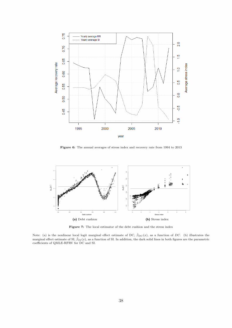
economy which only observed in the recent financial crisis (GFC). Figure 6 illustrates the

movement of the annual averages SI in the last decades, which reflects several economic

conditions such as Dot-Com crisis (1999 - 2003), economic expansion (2004-2006), as well

as the global financial crisis (2007-2010). The figure also shows the negative relationships

between SI and the recovery rate.

[————— Insert [ Figure 6] here—————]

Table 5 provides the summary statistics of each variable as well as the contingency

table of the covariates and the recovery rate. There are five determinants, of which three

categorical variables, types of loan, instrumental rank and collateral status (see Panel A

in Table 5), and two continuous variables DC and SI (see Panel B). In the first row, the

reported figures were the recovery rates at the 0.05, 0.25, 0.5, 0.75, and 0.95 quantiles.

The other rows indicate the frequency distributions of recovery rate conditional on each

category of categorical variables, followed by those conditional on discretised values of the

two continuous variables.

[————— Insert [Table 5] here —————]

Panel A(i), our data has five different types of the defaulted loans, where the data has

42% of commercial loans12 and 58% of bonds13. Considering the average RR of each type,

the revolving loan has the highest rate, while the junior and subordinate bonds are the

most risky types of loan with the lowest average of 0.24. We also find that the recovery

rates of the commercial loans and the senior secured bond tend to have negative skewness

11Federal Reserve Bank of St. Louis, St. Louis Fed Financial Stress Index c© [STLFSI], retrieved fromFRED, Federal Reserve Bank of St. Louis; https://fred.stlouisfed.org/series/STLFSI

12which are term loan and revolving loan13There are four types of the bonds defined by their seniority

17

compared to the remaining loans, due to the relatively high medians and high masses at

the upper quantiles.

The instrumental rank generally indicates the repayment priority in the capital struc-

ture14. Therefore, we find that the averages of the recovery rate decrease as Rank in-

creases, in Table 5, Panel A(ii). Also, as most commercial loans generally have Rank 1,

the contingency table shows that the RR densities of Rank 1 is similar to those of the

commercial loans.

Lastly, collateral is the main source of fund to repay the outstanding defaulted debt.

Panel A(iii) shows that the collateralised loan has substantial higher average recovery rate

than the uncollateralised loan. 50% of the uncollateralised loan can recover less than 20%

of the total loss, while more than a half of collateralised loans can recover more than 90%.

Panel B represents the preliminary analysis of the relationships the continuous vari-

ables and RR. First, we partition the defaulted loan based on the level of DC. Debt

Cushion, as suggested by Van de Castle and Keisman (1999), is a facility-level metric

that captures not only the rank of debt in capital structure, but the degree of its subor-

dination as a proportion of total claims. This, in turn, reflects the liquidity available for

a liquidation. Table 5 shows that 46% of the data has zero DC, where the average RR

of them is 0.4. If the DC is greater than 0.5, the average RR can be as high as 0.8, also

more than three fourth of them has almost full recovery on average, compared to 0.07 for

the loan with zero DC.

Lastly, the recovery rate is partitioned by the given levels of SI in Panel B(ii). We

denote the range of DC as negative SI, 0 < SI < 1, and SI ≥ 1, which represent low, high,

and substantial high stressed periods, respectively. Based on the average RR, the recovery

rate during the low stress is the lowest at 0.7, while the rates are similar at approximately

0.5 for high and substantial high stress periods. During the good economic condition,

more than a half of the defaulted loan can be recovered more than 80% of the total loss

compared to 40% for the otherwise periods. We, then, expect the negative effect of SI

on RR. It can be also notice that the densities of RR during high and extremely high

economic stress are distributed as similar as one another.

14To recover the defaulted loss after declared bankruptcy of the borrowers, their assets will be liquidatedand then allocated to repay the lenders, which is prioritised by the instrumental rank.

18

6 Empirical results

The local logit model is applied to RR dataset to uncover the nature of the underlying

unknown nonlinear RR-covariates relationship, conduct marginal and interaction effects

analysis, and generate RR predictions. The results of this empirical investigation will be

utilized to improve the specification of the parametric QMLE-RFRV model - calibrated

model.

6.1 Bandwidth selection

We estimate the local logit model for the full dataset of 3, 573 defaulted loans. The local

logit regression for the RR data is specified as:

y = E(Y |X = x) = Λ(x′β(x)

)= Λ

(β0(x) + βDC(x) ·DC + βSI(x) · SI

+6∑d=2

βType(d)(x) · Type(d) +4∑d=2

βRank(d)(x) ·Rank(d)

+ βCol(x) · Col),

(12)

where β(x) = (β0(x), βDC(x), ..., βCol(x))′ is a vector of unknown parameters, which are

functions of the entire set of covariates x. Type(d) and Rank(d) are dummy variables

representing each category of discrete variables Type and Rank, respectively; See Table

5 for more details. For a comparison purpose, we estimate the benchmark model which

is the standard linear QMLE-RFRV, denoted as Λ(x′γ).

The local logit parameters are estimated with the kernel function (5) for continuous

variables DC and SI, and kernel function (6) for categorical variables Type, Rank and Col.

The bandwidth is selected by the leave-one-out least-squares cross-validation method (7).

Let us define,

H = (h1, h2, `1),

where H is 3 × 1 vector of the bandwidths, h1 and h2 are associated with DC and SI,

respectively, and `1 is a single bandwidth for all three categorical variables: Rank, Type

and Col. H = (0.11, 1.27, 1.00) is the set of selected optimum bandwidths. We estimate

19

the local logit model with the selected bandwidths for the full dataset and find that MSE

of the local logit model is 0.076, whereas it is 0.089 for the benchmark model QMLE-

RFRV. The results indicate that the local logit is a better fit for the RR data than the

benchmark model.

6.2 Local logit analysis

The marginal effects of continuous variables and discrete variables are analysed in the

local logit and the parametric QMLE-RFRV models.

(i) Local logit estimates of continuous variables

[————— Insert [Figure 7] here —————]

Figure 7a shows the local logit estimate of DC is a nonlinear function of DC, denoted

as βDC(x), while the QMLE-RFRV estimate γDC represented by the solid horizontal line.

In the local logit model, the marginal effect on DC depends on the level of DC, whereas

it is constant in the parametric model.

In the local logit model, the effect of DC on RR increases somewhat linearly for

0 < DC < 0.6, reaching the highest impact when DC = 0.6, followed by a decreasing

effect on the RR of the defaulted loans for 0.6 ≤ DC < 0.8 reaching the lowest effect at

DC = 0.8. There onwards, the effect increases for DC > 0.8. These results imply that the

defaulted loans with 0 < DC < 0.6 tend to be more effectively responsive to an increase

in additional DC than the loan with higher DC. In comparison to the parametric estimate

of 2.5, the effect of DC on RR is mostly positive as expected and the average local logit

estimate βDC(x) is also close to 2.5 (Figure 7a).

To analyze the effect of SI on RR, βSI(x) and γSI are plotted (solid line) in Figure

7b. To explain the marginal effect of SI on RR, we consider three ranges of the SI: low

SI as SI<0, high SI as 0 < SI < 1.5, and the crisis SI as SI > 1.5, indicating good, poor

and (global financial) crisis economic conditions. The effect of SI on RR is negative and

increasing with SI and then it becomes positive and increasing for SI > 1.5. The variation

of the effect of SI on RR is very high for the low values of SI. This result indicates

that RR is more sensitive to the change in the economic conditions during the low SI

20

period, compared to high SI and the crisis. The variation of the local logit estimate shows

that although SI has a nonlinear negative effect on RR, the magnitude of the effects are

different depending on the characteristics of each loan. The relatively small variation of

the local estimate observed for high SI implies that the effect of high SI is less dependent

on the loan characteristics than for the low SI and the crisis SI. In practice, these findings

indicate by the change in behavior and expectations of both banks and borrowers during

the economic downturn (0 < SI ≤ 1.5). Lenders would have similarly adopted more

conservative financial strategies preparing to a pessimistic scenario. This leads to the

smaller negative effect of high SI on RR with lower variation.

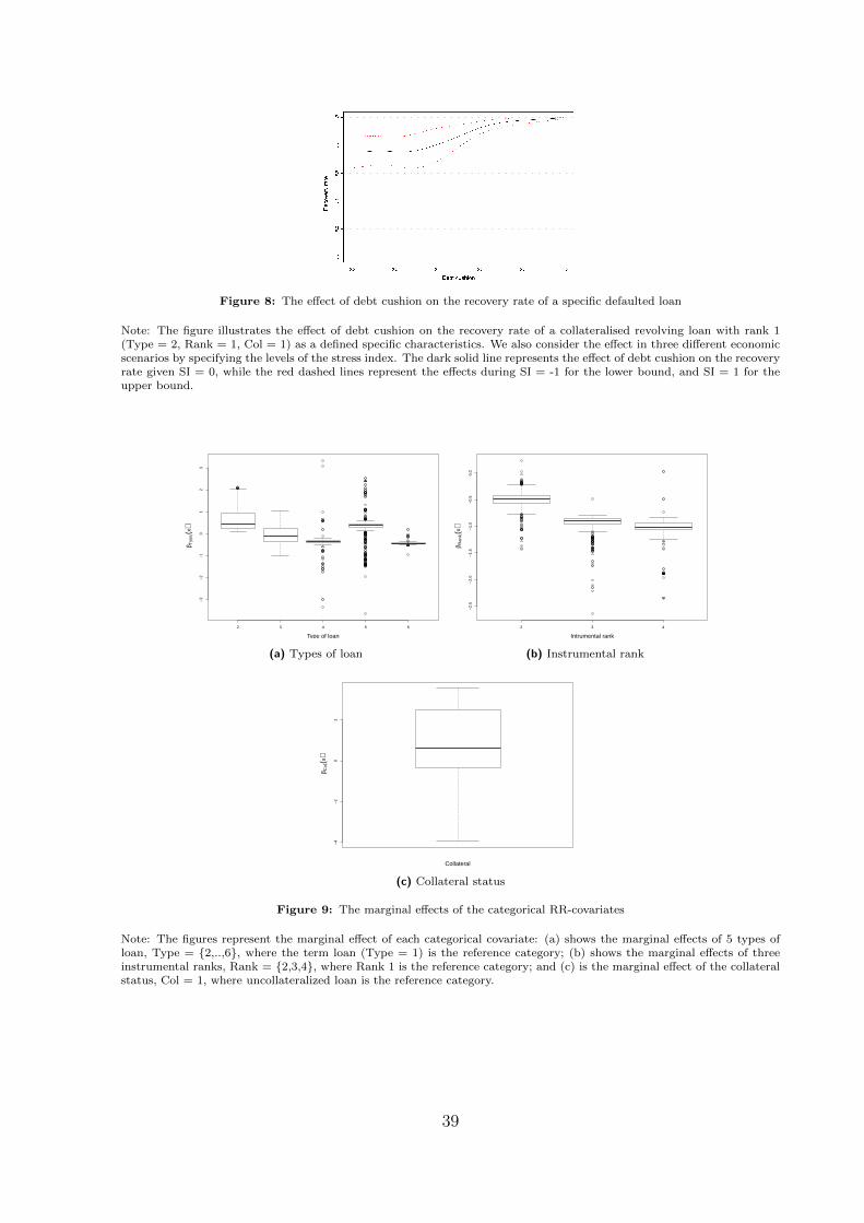
[————— Insert [Figure 8] here —————]

Furthermore, we consider SI = {−1, 0, 1} and study the effect of DC on RR for the

loans with (Type = 2, Rank = 1, Col = 1) across various economic conditions measured

by SI. The plot in Figure 8 indicates the RR is nonlinear function of DC. The marginal

effect of DC on RR is zero for DC < 0.3, and positive & increasing until DC = 0.6, and

then nearly zero for DC > 0.6. On the other hand, SI has a negative impact on RR.

For example, if we consider a loan with DC = 0, then the RR is 0.63, 0.75, and 0.90

respectively for high stress period (SI = 1), neutral period (SI = 0), and low stress period

(SI = -1) respectively. Figure 8 also shows that the negative effect of SI on the loan with

low DC is stronger than the loan with higher DC, as RR of the given loan with DC = 1 is

approximately one for all levels of SI. The loan with high level of DC is not very sensitive

to the change in the economic condition compared to that with the lower DC.

(ii) Local estimates of discrete variables

We turn to the analysis of the local estimates of the discrete variables including type of

loan; instrumental rank; and collateral status. The estimates indicate the levels of riski-

ness of each category in comparison to the reference category15. Specifically, a negative

estimate means the category of interest has lower RR (higher risk) than the reference

category, given other variables held constant.

Table 6 compares the median of local logit estimates of all discrete variables with the

coefficients estimates of QMLE-RFRV. The result shows that the median of the local

estimates and the QMLE-RFRV estimates are more or less the same. These results imply

15The reference categories of Type, Rank and Col are given in Table 5

21

that the local estimators for the discrete variables contain somewhat similar information

as the parametric estimators.

[————— Insert [Table 6 ] here —————]

The local logit estimates of all discrete variables are presented in Figure 9 and their

signs are mostly in line with expectation. However, there are some unexpected positive

estimates for the local estimates of senior secured bond (Type 3), senior unsecured bond

(Type 5) in Figure 9a; and unexpected negative estimates for Col in Figure 9c. In general,

both types of senior bonds are expected to have lower RR than the term loan due to the

priority in the credit capital structure, hence only a negative sign is expected. On the

other hand, the collateralised loan is commonly expected to have a higher RR than the

loan without collateral, then the positive effect is expected. As shown earlier in the

simulation study, the unexpected signs of the estimates maybe due to the presence of

potential interaction effects.

[————— Insert [Figure 9 ] here —————]

We find that there are some significant relationships between DC and both local es-

timates of Type = {3,5} and Col = 1. Figure 10 shows that the effects of both senior

bonds are highly dependent on the levels of DC, which indicate the interactions between

DC and both senior bonds. First, for the senior secured bond, Figure 10a shows that

the unexpected positive estimates for the defaulted loan with 0.2 < DC < 0.6. Second,

for the senior unsecured bond, the expected negative signs are observed only for the loan

with 0.1 < DC < 0.5 in Figure 10b.

[————— Insert [Figures 10 and 11 ] here —————]

To explain the unexpected negative estimate of Col, see Figure 11 which shows the

relationship between the local estimates of Col and the levels of DC. The clear pattern

emerges in Figure 11a, the estimates are negative, when the defaulted loan has DC between

0.2 and 0.5.

In Table 7, we report the results of the partitioning empirical RR data based on the

findings of the interaction effect analysis. The result confirms that the local logit analysis

can uncover the some underlying true interaction effects observed in the empirical data.

For example, in Panel A, we compare the average RR of the senior secured bond with

those of the collateralized term loan (reference category) for various ranges of DC . We

find that, although the average RR of the term loan is mostly higher than that of senior

22

secured bond, only the bond with 0.2 ≤ DC < 0.6 has a higher RR than the term loan.

This finding is consistent with the positive local logit estimate of the senior secured bond

plotted in Figure 10a.

[————— Insert [Table 7 ] here —————]

6.3 Calibrated QMLE regression for fractional response variable

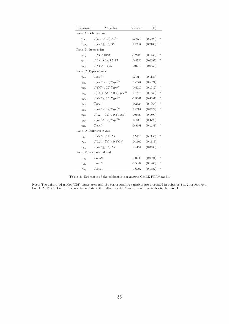
Table 8 reports the estimates of the improved specification of the QMLE-RFRV - cali-

brated model. The variables and interaction terms (Column 2 of Panels A, B, C and D,

Table 8) of the calibrated model were obtained from the results of local logit analysis16.

In Panel B, the parameter estimates of γSI1 , γSI2 , and γSI3 represent the effects of SI

for low SI, high SI and the crisis SI, respectively. The results show that negative effects

are the strongest for the low SI followed by the high SI, and the effect becomes insignifi-

cant during the crisis SI, which is consistent with our previous findings in the local logit

analysis. Furthermore, the interaction effects between DC and the senior secured bond

are captured by the parameters γT31 , γT32 , and γT33 in Panel C. The results show that

only γT32 estimate is significantly positive, which represents the interaction effect between

senior secured bond and DC ∈ [0.2, 0.6). This means that the senior secured bond with

0.2 ≤ DC < 0.6 is likely to have higher RR than the term loan, which is consistent with

our previous findings in local logit model. These results show that the behaviours of the

parameter estimates in the calibrated model are more or less the same as those of the the

local logit estimates.

[————— Insert [Table 8 ] here —————]

Moreover, we test the null hypothesis that the calibrated QMLE-RFRV fits the data

against the alternative hypothesis that the local logit fits the data well, by applying

the wild bootstrap-based specification test with 1,000 iterations. The calibrated QMLE-

RFRV model (Table 8) is not rejected at the 5% nominal level, as the p-value computed

by the bootstrap method 0.09. This test provides statistical evidence that the calibrated

model specification fits the RR data well.

16We also found the interaction term between Type = 2 and DC.

23

6.4 Out-of-sample predictive performance

In this section, we compared the out-of-sample predictability of the local logit model, the

calibrated QMLE-RFRV model and the standard QMLE-RFRV model. In this study,

we evaluate the point predictive and the quantile predictive performances of these three

models.

6.4.1 Predictive performance criteria

Point prediction evaluation

We use three methods to partition the full samples into in- and out-of-samples and assess

the sensitivity of the models’ predictions to these methods. The three methods include:

(DF1) Partition the full sample randomly into pre-specified 70:30 ratio of in-sample:out-

of-sample, for 1,000 iterations. Although, this is a standard evaluation of out-of-

sample prediction, the overfitting issue is not properly addressed. According to our

empirical RR data, one borrower could have several defaulted loans. By randomly

partition the full data, it allows the overlapping information, as the information of a

borrower could be in both in- and out-of-sample data. This leads to the overfitting

problem (Kalotay & Altman, 2016).

(DF2) Partition the full sample into, for example, the in-sample period 1994-2005, and

the out-of-sample period 2006-2012. This way of partitioning ensures that there is

no overlapping observations in the both samples. This definition also mimics the

application of RR predictive model in practice, as banks would want to use the full

observed data to predict RR in the forthcoming years.

(DF3) Select any particular year as the out-of-sample period, and the remaining years as

the in-sample period. For example, the out-of-sample period is the start of the

GFC, 2008, then the in-sample period is 1994-2007 and 2009-2012. This way of

partitioning the in- and out-of-sample is very useful to predict RR at the various

phases of the economic cycle.

Quantile prediction evaluation

In this method, we evaluate the predictive performance of the models at various quantiles

24

of the simulated RR portfolio distribution of the out-of-sample; see Altman and Kalotay

(2014) for details. The following re-sampling procedure is employed to construct the RR

portfolio distribution:

(i) Define the in-sample data period 1994-2004 and the out-of-sample period 2004-2012

(ii) Draw a random sample of 100 RRs from the out-of-sample data with replacement.

Assign each loan a $1.00 face value and construct an equally-weighted portfolio of

the selected RRs. This RR portfolio represents the money that is recovered from

$100.00 portfolio’s face value.

(iii) Predict the selected out-of-sample RR by the benchmark QMLE-RFRV model, local

logit model, and calibrated QMLE-RFRV model. Then, the predicted RR portfolio

is constructed for each model

(iv) Repeat (ii) and (iii) above 10,000 times and construct a simulated RR portfolio

distributions for the three models under investigation

The model performance is evaluated by the predictive error of the simulated RR

portfolio at various quantiles of the distribution.

6.4.2 Comparison of predictive performances

Point prediction accuracy

We adopt the data partitioning method DF1, the out-of-sample MSE and MAE of the

local logit model are 0.0824 and 0.2750, respectively. For the calibrated linear model,

they are 0.0854 and 0.2880, receptively. On the other hand, the benchmark model has

the highest predictive errors, 0.0964 and 0.3246. These results indicate that the local logit

model outperforms others.

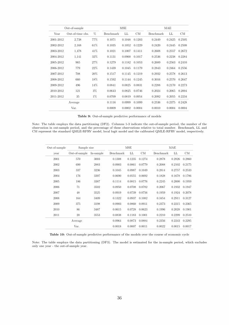
The results of the out-of-sample evaluation of the models for DF2 are reported in

Table 9, which include the predictive performances of 11 different out-of-sample windows

from 2001 to 2012. For the first window, we estimate the models for the in-sample period

1994 to 2000, and evaluate the predictions of out-of-sample period 2001 to 2012. Then,

the in-sample window is continually expanded by each calendar year until the eleventh

window in-sample period is 1994 to 2010 and the out-of-sample period is only 2011-2012.

The MSE and MAE of the predictions for each window are reported in Table 9.

25

[————— Insert [Table 9] here —————]

The result shows that the proposed local logit model has the highest predictive accu-

racy, followed by the calibrated model. The benchmark model outperforms the proposed

model only in the two out-of-sample windows of 2002-2012 and 2010-2012 under the both

MSE and MAE criteria at the 5% level of significance (Table 9). This table also provides

the average and variance of MSE and MAE over 11 windows. The MSE and MAE av-

erages of the proposed local logit model as well as their variances are consistently lower

than those of the benchmark model.

Noticeably, the differences in MSE among three models are large for the out-of-sample

predictions between 2004 and 2008 in Table 9. These years are crucial, since they partially

cover the global financial crisis period 2007 to 2010. The benchmark model is highly

sensitive to the crisis year compared to the non-parametric and the calibrated models.

The MSE and MAE are very large during the crisis period for the benchmark model. The

low accuracy of the benchmark model during the GFC could be due to the unexpected

shock with substantially high level of SI. As a linear model, the constant negative effect

of SI could lead to the underprediction of RR during the crisis.

[————— Insert [Table 10] here —————]

The results of the point prediction evaluations of the three models for DF3 are pre-

sented in Table 10, where we predict RR every year from 2000 to 2011. Table 10 shows

that the local logit regression consistently outperforms the benchmark regression. The

MSE and MAE averages of the proposed model across 11 years are 0.087 and 0.224, com-

pared to 0.096 and 0.235 for the benchmark model. The benchmark model prediction

outperforms the proposed model only in 2010 and 2011. The calibrated model mostly

outperforms the benchmark model and its performance is comparable to that of local

logit model. As far as the economic cycle is concerned, the local logit model and the

calibrated QMLE-RFRV model have comparable performance and outperform the bench-

mark model at all window sizes, and the MSEs of those former models are substantially

lower than the benchmark model during the GFC period. On the other hand, we observe

that the benchmark model yields relatively high MSE during the recent GFC periods

(2007-2009) when SI level is at its peak.

26

Quantile prediction accuracy

We evaluate the performances of the models at various quantiles of the simulated portfolio

distribution. The results in Table 11 compare RRs at the 0.05, 0.25, 0.5, 0.75, and 0.95

quantiles of the observed RR portfolio distribution with those of the predicted portfolio

distributions. The local logit model and the calibrated model predict RR portfolio at

the five selected quantiles of the distribution more precisely than the benchmark model.

For example, at the 0.5 quantile of the portfolio distribution, the actual portfolio can

recover $63.96 from $100.00 face value, while the predictions by the both proposed model

and the calibrated model are approximately $61.30 compared to the benchmark model

prediction of $67.71. This implies that the benchmark model is more likely to overestimate

the RR portfolio value compared to other two models. Also we find that the local logit

outperforms the other models for the high risk portfolios (at the low quantiles) followed

by the calibrated model.

[————— Insert [Table 11] here —————]

In summary, the proposed local logit model outperforms the other two models as

indicated by all predictive performance measure criteria by the both point and quantile

predictions. We also find that the calibrated model has slightly lower predictability than

the proposed model, and outperforms the benchmark model.

7 Conclusion

In this study, we propose a nonparametric local logit model for [0,1] bounded response

variable, assess their finite sample properties relative to the QMLE regression for fractional

response variable (QMLE-RFRV) - the benchmark model. These two models are then

applied to empirical RR data and covariates. The results of the marginal and interaction

effect analyses of the local logit model are utilised to calibrate the QMLE-RFRV model.

The in-sample and out-of sample predictive performances of the three models are assessed

using MSE and MAE measures. The main findings of this study are the following:

First, an extensive simulation study establishes that the properties of local logit model

estimates are as good as than the correctly specified parametric model in moderate sam-

ple sizes and they are robustness to asymmetric and bimodal error distributions. Second,

we apply local logit regression to model RR data, which uncovers the underlying nonlin-

27

ear RR data and covariates relationship including interaction effects among covariates.

Third, we exploit the results of local logit model to improve the parametric QMLE-RFRV

model specification, which we call calibrated model. The calibrated model is nonlinear in

variables which includes some useful interaction terms. Fourth, we assess the in-sample

and the out-of-sample RR predictability of the local logit model and the calibrated model

in comparison to the standard parametric model. The results show that the local logit

model outperforms the others. In addition, the calibrated model is comparable to local

logit model in the predictive performance. An attractive feature of the local logit and

calibrated models is that they outperform the benchmark model in the out-of-sample RR

prediction during the crisis period. Our findings are useful to applied researchers and

practitioners who are unfamiliar with the nonparametric machinery, and banks to design

treatment program for their borrowers.

Appendix A: Simulations results

Tables and figures

n = 200In-sample Out-of-sample

Benchmark LL Benchmark LL

Specification MSE MAE MSE MAE MSE MAE MSE MAE

U1 0.0156 0.0720 0.0156 0.0720 0.0161 0.0722 0.0161 0.0722

U2 0.0195 0.0825 0.0182 0.0811 0.0199 0.0825 0.0200 0.0831

U3 0.0325 0.1362 0.0312 0.1361 0.0331 0.1382 0.0333 0.1399

B1 0.0211 0.1022 0.0211 0.1022 0.0215 0.1028 0.0215 0.1028

B2 0.0312 0.1299 0.0298 0.1299 0.0314 0.1300 0.0322 0.1312

B3 0.0260 0.1109 0.0234 0.1102 0.0256 0.1129 0.035 0.1271

Table 1: In-sample and out-of-sample predictions of models in the simulation study with small sample size

Note: The benchmark model is the standard QMLE-RFRV. The local logit regression is denoted as LL

28

n = 500In-sample Out-of-sample

Benchmark LL Benchmark LL

Specification MSE MAE MSE MAE MSE MAE MSE MAE

U1 0.0121 0.0682 0.0121 0.0682 0.0112 0.0691 0.0112 0.0691

U2 0.0191 0.0841 0.0187 0.0827 0.0181 0.0811 0.0182 0.0811

U3 0.0333 0.1355 0.0326 0.135 0.0325 0.1386 0.0326 0.1388

B1 0.2041 0.0958 0.2041 0.0958 0.0207 0.1005 0.0207 0.1005

B2 0.0309 0.1255 0.0301 0.1256 0.0313 0.1291 0.0314 0.1300

B3 0.0261 0.11 0.0241 0.1021 0.0252 0.1123 0.0259 0.1151

M1 0.1100 0.2731 0.109 0.2722 0.1154 0.2781 0.1162 0.2812

Table 2: In-sample and out-of-sample predictions of models in the simulation study with moderate sample size

Note: The benchmark model is the standard QMLE-RFRV. The local logit regression is denoted as LL

Relative mean squared error

n = 200 n = 500 n= 1000

Error (U) distribution Benchmark LL Benchmark LL Benchmark LL

Panel (a): In-sample prediction

Specification: M1

Chi-square 1.9618 0.7603 1.8828 0.9218 1.8645 0.9773

Bimodal 1.0893 1.1003 1.0844 0.9592 1.0839 0.9838

Specification: M2

Chi-square 1.3811 0.9206 1.3685 0.8512 1.1466 0.9857

Bimodal 1.0615 1.0392 1.0600 1.0296 1.0569 0.9350

Panel (b): Out-of-sample prediction

Specification: M1

Chi-square 1.9178 1.4636 1.9816 1.2444 1.9005 1.1072

Bimodal 1.0854 1.1191 1.0800 1.0501 1.0750 1.0304

Specification: M2

Chi-square 1.3727 1.4701 1.3553 1.2094 1.3713 1.1466

Bimodal 1.0491 1.0835 1.0572 1.0503 1.0527 1.0464

Table 3: The mean square error of the local logit model relative to correctly specified QMLE-RFRV model

Note: The benchmark model is the standard linear QMLE-RFRV model. LL is the proposed local logit model. The relativeMSE is the MSE of the given model relative to the correctly specified QMLE-RFRV model. The error U(1) ∼ χ2

(1)-

asymmetric distribution. The error U(2) generated from the equally weighted mixture of N(−2, 1) and N(2, 1) - bimodaldistribution.

29

Relative mean absolute error

n = 200 n = 500 n= 1000

Error (U) distribution Benchmark LL Benchmark LL Benchmark LL

Panel (a): In-sample prediction

Specification: M1

Chi-square 1.5536 0.8819 1.5366 0.9959 1.5341 1.0272

Bimodal 1.0664 1.0524 1.0622 0.9962 1.0627 1.0131

Specification: M2

Chi-square 1.2464 0.9099 1.2410 0.9089 1.2370 1.0050

Bimodal 1.0408 1.0148 1.0413 1.0250 1.0380 0.9618

Panel (b): Out-of-sample prediction

Specification: M1

Chi-square 1.5434 1.1824 1.5612 1.1310 1.5219 1.0807

Bimodal 1.0627 1.0597 1.0594 1.0412 1.0563 1.0357

Specification: M2

Chi-square 1.2376 1.1679 1.2301 1.0880 1.2440 1.0859

Bimodal 1.0364 1.0404 1.0397 1.0356 1.0360 1.0219

Table 4: The mean absolute error of the local logit model relative to correctly specified QMLE-RFRV model

Note: The benchmark model is the standard linear QMLE-RFRV model. LL is the proposed local logit model. The relativeMAE is the MAE of the given model relative to the correctly specified QMLE-RFRV model. The error U(1) ∼ χ2

(1)-

asymmetric distribution. The error U(2) generated from the equally weighted mixture of N(−2, 1) and N(2, 1) - bimodaldistribution.

2 4 6 8 10

−3

−2

−1

01

23

X1

Loca

l Log

it E

stim

ator

(a) Local logit regression, D2 = 0

2 4 6 8 10

−3

−2

−1

01

23

X1

Loca

l Log

it E

stim

ator

(b) Local logit regression, D2 = 1

2 4 6 8 10

−3

−2

−1

01

23

X1

QM

LE−

RF

RV

Est

imat

or

(c) QMLE-RFRV, D2 = 0

2 4 6 8 10

−3

−2

−1

01

23

X1

QM

LE−

RF

RV

Est

imat

or

(d) QMLE-RFRV, D2 = 1

Figure 1: The interaction effects estimates of x1 conditional on d2 under simulation M1

Note: These figures show the interaction effect estimates of x1 and d2 for the simulation assumption M1. (a) and (b)illustrate the local logit marginal effect estimates β1(x) as a function of x1 conditional on d1 = 0 and 1, respectively,as specified in (10). On the other hand, (c) and (d) represent the parametric QMLE-RFRV estimates γ1 and γ1 + γ6,respectively, as specified in (9).

30

−1 0 1 2 3

−2

−1

01

2

X2

Loca

l Log

it E

stim

ator

(a) Local logit regression

−1 0 1 2 3

−2

−1

01

2

X2

QM

LE−

RF

RV

Est

imat

or

(b) QMLE-RFRV

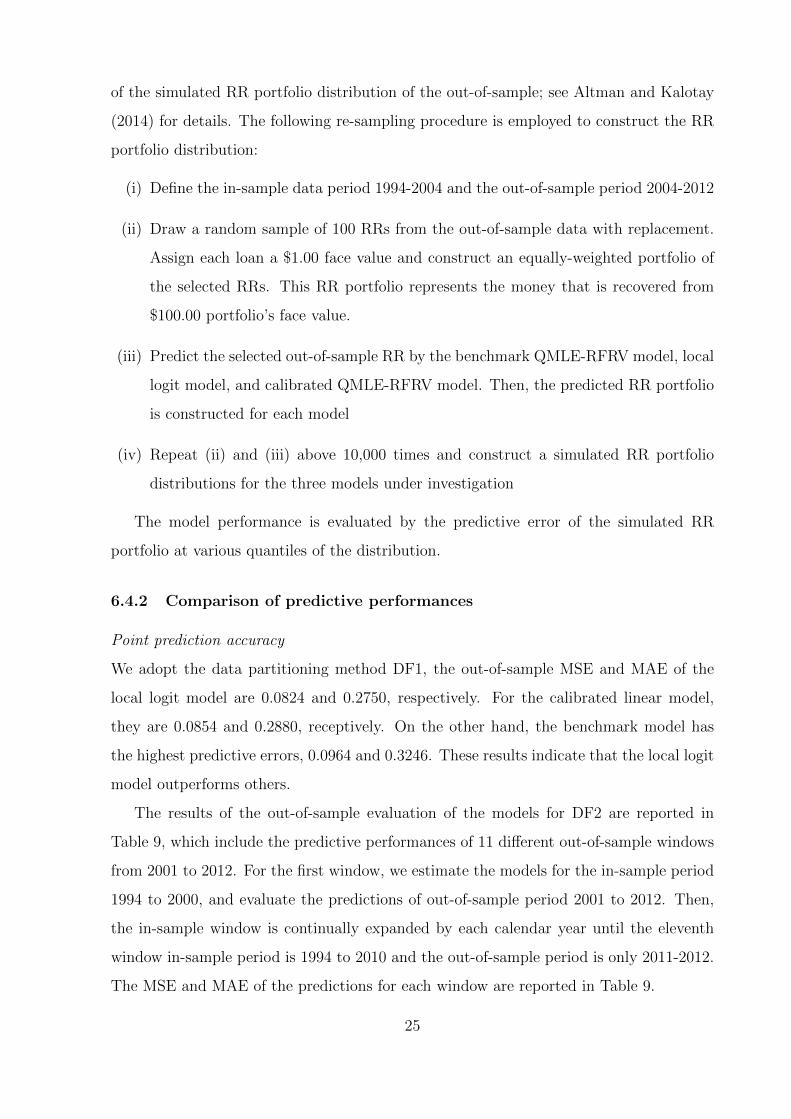
Figure 2: The nonlinear marginal effect estimates of x2 under simulation M1

Note: (a) is the local logit marginal effect estimate β2(x) in (10) as a function of x2. (b) represents the parametricQMLE-RFRV estimate γ2 cos(x2) as the marginal effect estimate of x2 in (9).

QMLE−RFRV Local Logit

−0.

50.

00.

51.

01.

52.

0

Est

imat

or (

D1)

(a) D1

QMLE−RFRV Local Logit

−0.

50.

00.

51.

01.

52.

0

Est

imat

or (

D3)

(b) D3

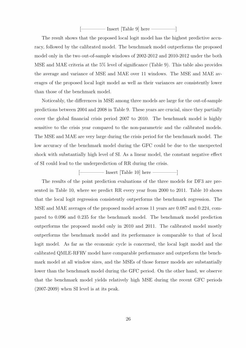
Figure 3: The marginal effect estimates of D1 and D3 under simulation M1

Note: (a) and (b) compare the marginal effect estimates of QMLE-RFRV and the local logit model for the discrete variablesD1 and D3 under simulation assumption M1 in (9) and (10). (a) represents the marginal effect estimates of D1, which

compares γ3 and β3(x), on the left and right hand sides of the figure, respectively. Similarly, (b) represents the comparison

of the marginal effect of D3 between γ5 and β5(x).

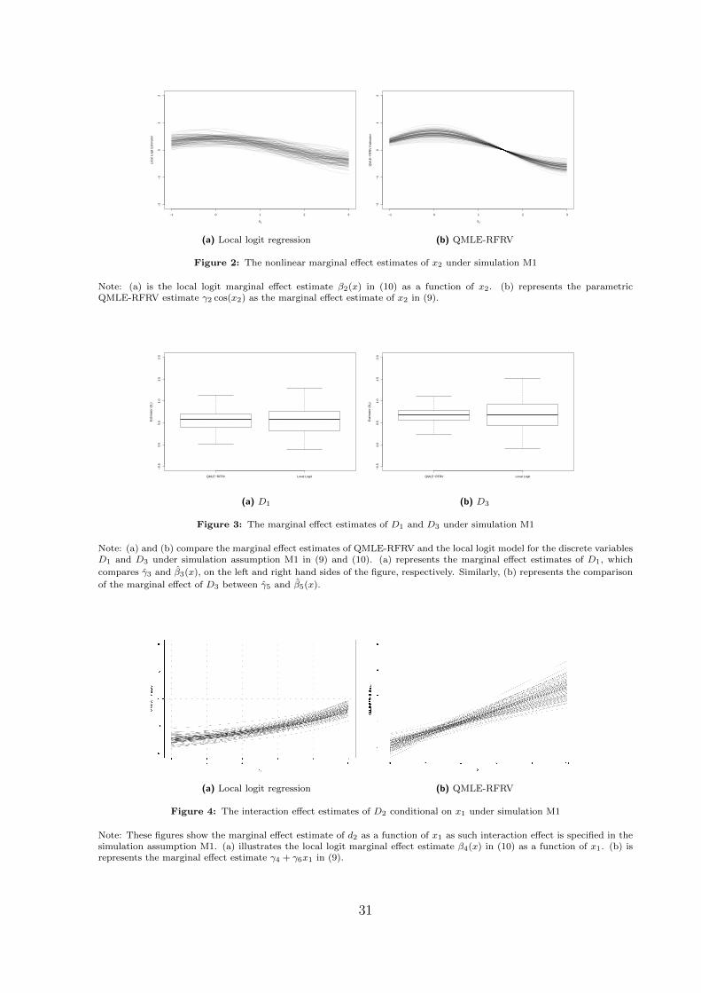
(a) Local logit regression (b) QMLE-RFRV

Figure 4: The interaction effect estimates of D2 conditional on x1 under simulation M1

Note: These figures show the marginal effect estimate of d2 as a function of x1 as such interaction effect is specified in thesimulation assumption M1. (a) illustrates the local logit marginal effect estimate β4(x) in (10) as a function of x1. (b) isrepresents the marginal effect estimate γ4 + γ6x1 in (9).

31

Appendix B: Empirical results

Tables and figures

Recovery rate at τ -quantile

Variables Frequency % Mean 5% 25% 50% 75% 95%

Recovery rate 3,573 100% 0.5570 0.0000 0.1849 0.5888 1.0000 1.0000

Panel A: Discrete Variables

(i) Type of loans

Term loans (Type(1) - reference category) 746 21% 0.7054 0.0222 0.4343 0.8638 1.0000 1.0000

Revolving loans (Type(2)) 738 21% 0.8251 0.2147 0.6934 1.0000 1.0000 1.0000

Senior secured bonds (Type(3)) 446 12% 0.5896 0.1079 0.2093 0.5682 1.0000 1.0000

Senior subordinated bonds (Type(4)) 355 10% 0.2429 0.0000 0.0080 0.1005 0.3779 0.9225

Senior unsecure bonds (Type(5)) 1,061 30% 0.4263 0.0000 0.1027 0.3578 0.7257 1.0000

Junior and subordinate bonds (Type(6)) 227 6% 0.2352 0.0000 0.0000 0.0968 0.3491 1.0000

(ii) Instrument rank

Rank(1) (reference category) 1,711 48% 0.7476 0.1221 0.5151 1.0000 1.0000 1.0000

Rank(2) 1,258 35% 0.4294 0.0000 0.1159 0.3170 0.7422 1.0000

Rank(3) 393 11% 0.2994 0.0000 0.0041 0.1531 0.5255 1.0000

Rank(4) 211 6% 0.2514 0.0000 0.0010 0.1027 0.3615 0.9122

(iii) Collateral

Uncollaterized loans (reference category) 1,712 48% 0.3685 0.0000 0.0396 0.2372 0.6638 1.0000

Collaterized loans 1,861 52% 0.7303 0.1240 0.4545 0.9622 1.0000 1.0000

Panel B: Continuous variables

(i) Debt Cushion (DC)

DC = 0 1,631 46% 0.3969 0.0000 0.0738 0.2840 0.6959 1.0000

0 < DC < 0.5 1,049 29% 0.5345 0.0043 0.2092 0.5476 0.8961 1.0000

0.5 < DC < 1 893 25% 0.8766 0.2386 0.9435 1.0000 1.0000 1.0000

(ii) Stress index (SI)

SI ≤ 0 853 24% 0.7058 0.0022 0.4728 0.8585 1.0000 1.0000

0 < SI < 1 2,272 63% 0.5102 0.0000 0.1533 0.4654 1.0000 1.0000

SI ≥ 1 448 12% 0.5105 0.0000 0.1344 0.4617 1.0000 1.0000

Table 5: Summary statistics and a contingency table of the empirical recovery rate data

Note: The full data is partitioned to several sub-samples by the given variables in the column 1, then columns 2 and 3report the number of the observation in each sub-sample and its percentage to the total observation, respectively. Columns4 to 9 is a contingency table, which indicates the RR density of each sub-sample.

32

VariablesParametric

coefficients (γ)

Median of

local logit coefficients (β(x))

Type of loan

Type(2) 0.4907*** 0.4376

(0.1358)

Type(3) -0.0229 -0.0328

(0.1433)

Type(4) -0.3771 -0.3857

(0.2331)

Type(5) 0.2535 0.2899

(0.2010)

Type(6) -0.4258 -0.4417

(0.2476)

Rank

Rank 2 -0.4512*** -0.5076

(0.1049)

Rank 3 -0.7900*** -0.8919

(0.1506)

Rank 4 -0.9300*** -1.0193

(0.1896)

Collateral

Collateralized loan 0.4420** 0.6127

(0.1842)

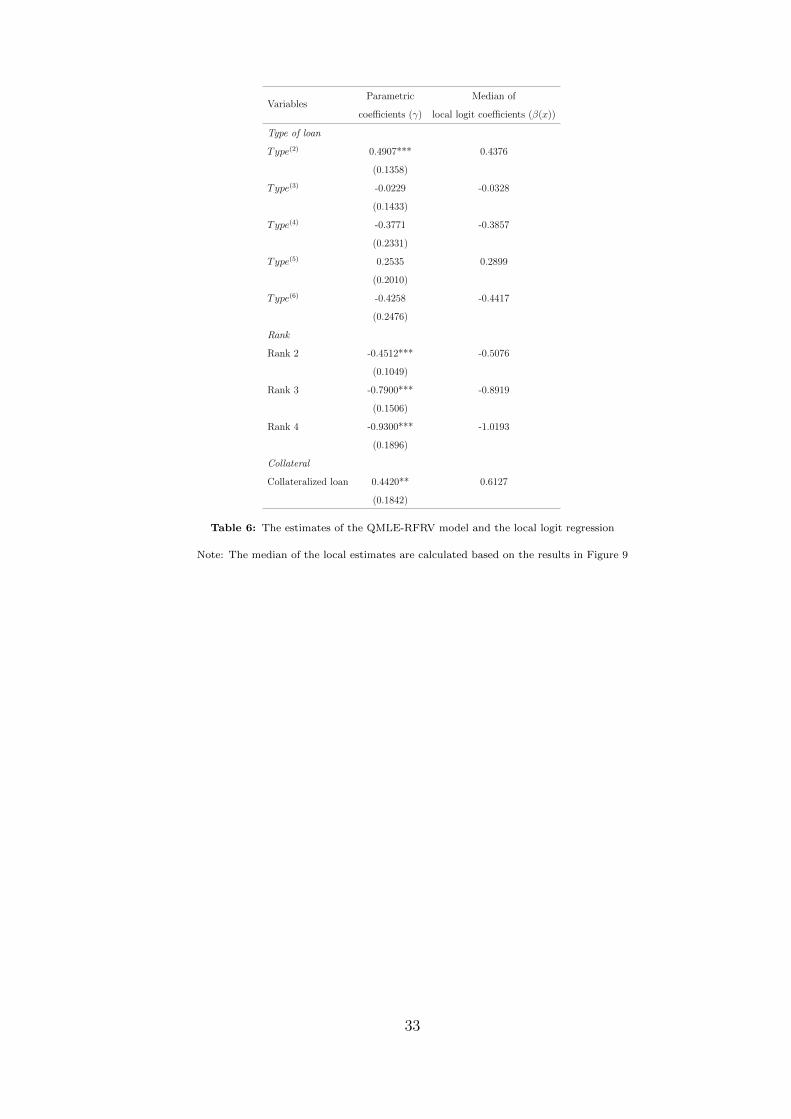
Table 6: The estimates of the QMLE-RFRV model and the local logit regression

Note: The median of the local estimates are calculated based on the results in Figure 9

33

Variables LL estimatesSample averages RR

Category of interest Reference category

Panel A Senior secured bond

DC ∈ [0, 1] N/A 0.59 0.71

DC < 0.2 Negative 0.44 0.53

0.2 ≤ DC < 0.6 Positive 0.82 0.71

DC ≥ 0.6 Negative 0.79 0.91

Panel B Senior unsecured bond

DC ∈ [0, 1] N/A 0.43 0.71

DC < 0.2 Positive 0.41 0.34

0.2 ≤ DC < 0.5 Negative 0.47 0.74

DC ≥ 0.5 Positive 0.77 0.36

Panel C Loans with collateral

DC ∈ [0, 1] N/A 0.73 0.37

DC < 0.2 Positive 0.53 0.31

0.2 ≤ DC < 0.5 Negative 0.68 0.63

DC ≥ 0.5 Positive 0.92 0.65

Table 7: The average recovery rates of senior bonds and collateralized loans for various ranges of DC

Note: The empirical RR is partitioned based on the findings in the interaction analysis of local logit model estimates ofsenior bonds and collateral status. Then RR of each sub-sample is compared with the reference group. For Panels Aand B, given the ranges of DC in the first column, the categories of interest are the senior secured and unsecured bonds,respectively, and the reference categories are collateralized and uncollateralized term loans, respectively. For Panel C, thethe category of interest is the collateralized loan, whereas the reference category is the uncollateralized loan.

34

Coefficients Variables Estimates (SE)

Panel A: Debt cushion

γDC1 I(DC < 0.6)DC2 5.5071 (0.5890) *

γDC2 I(DC ≥ 0.6)DC 2.4200 (0.2105) *

Panel B: Stress index

γSI1 I(SI < 0)SI -1.2283 (0.1436) *

γSI2 I(0 ≤ SI < 1.5)SI -0.4589 (0.0997) *

γSI3 I(SI ≥ 1.5)SI -0.0212 (0.0330)

Panel C: Types of loan

γT21 Type(2) 0.0817 (0.1124)

γT22 I(DC > 0.8)Type(2) 0.2770 (0.5021)

γT31 I(DC < 0.2)Type(3) -0.4516 (0.1912) *

γT32 I(0.2 ≤ DC < 0.6)Type(3) 0.8757 (0.1883) *

γT33 I(DC ≥ 0.6)Type(3) -1.5847 (0.4087) *

γT41 Type(4) -0.3635 (0.1265) *

γT51 I(DC < 0.2)Type(5) 0.2713 (0.0574) *

γT52 I(0.2 ≤ DC < 0.5)Type(5) -0.0456 (0.1806)

γT53 I(DC ≥ 0.5)Type(5) 0.8014 (0.4795)

γT61 Type(6) -0.3691 (0.1431) *

Panel D: Collateral status

γC1 I(DC < 0.2)Col 0.5802 (0.1733) *

γC2 I(0.2 ≤ DC < 0.5)Col -0.1600 (0.1383)

γC3 I(DC ≥ 0.5)Col 1.2458 (0.3536) *

Panel E: Instrumental rank

γR2 Rank2 -1.0040 (0.0901) *

γR3 Rank3 -1.5447 (0.1204) *

γR4 Rank4 -1.6792 (0.1422) *

Table 8: Estimates of the calibrated parametric QMLE-RFRV model

Note: The calibrated model (CM) parameters and the corresponding variables are presented in columns 1 & 2 respectively.Panels A, B, C, D and E list nonlinear, interactive, discretised DC and discrete variables in the model

35

Out-of-sample MSE MAE

Year Out-of-time obs. % Benchmark LL CM Benchmark LL CM

2001-2012 2,738 77% 0.1071 0.1048 0.1203 0.2449 0.2425 0.2505

2002-2012 2,168 61% 0.1035 0.1052 0.1229 0.2420 0.2445 0.2508

2003-2012 1,478 41% 0.1021 0.1007 0.1411 0.2608 0.2557 0.2672

2004-2012 1,141 32% 0.1131 0.0900 0.1017 0.2536 0.2238 0.2284

2005-2012 965 27% 0.1279 0.1182 0.1053 0.2689 0.2563 0.2410

2006-2012 779 22% 0.1439 0.1045 0.1179 0.2843 0.2464 0.2556

2007-2012 708 20% 0.1517 0.1145 0.1219 0.2932 0.2578 0.2613

2008-2012 660 18% 0.1592 0.1144 0.1245 0.3016 0.2570 0.2647

2009-2012 496 14% 0.0841 0.0825 0.0831 0.2288 0.2170 0.2273

2010-2012 121 3% 0.0643 0.0825 0.0746 0.2024 0.2065 0.2004

2011-2012 35 1% 0.0709 0.0819 0.0954 0.2092 0.2055 0.2234

Average 0.1116 0.0999 0.1099 0.2536 0.2375 0.2428

Var. 0.0009 0.0002 0.0004 0.0010 0.0004 0.0004

Table 9: Out-of-sample predictive performance of models

Note: The table employs the data partitioning (DF2). Columns 1-3 indicate the out-of-sample period, the number of theobservation in out-sample period, and the percentage of these observations relative to total number. Benchmark, LL andCM represent the standard QMLE-RFRV model, local logit model and the calibrated QMLE-RFRV model, respectively.

Out-of-sample

year

Sample size MSE MAE

Out-of-sample In-sample Benchmark LL CM Benchmark LL CM

2001 570 3003 0.1308 0.1235 0.1274 0.2878 0.2826 0.2860

2002 690 2883 0.0903 0.0861 0.0779 0.2088 0.2102 0.2175

2003 337 3236 0.1045 0.0987 0.1049 0.2814 0.2757 0.2533

2004 176 3397 0.0690 0.0555 0.0692 0.1828 0.1678 0.1786

2005 186 3387 0.1114 0.0815 0.0776 0.2245 0.2000 0.1959

2006 71 3502 0.0950 0.0708 0.0782 0.2067 0.1932 0.1947

2007 48 3525 0.0919 0.0739 0.0756 0.1959 0.1924 0.2078

2008 164 3409 0.1322 0.0937 0.1082 0.3454 0.2911 0.3127

2009 375 3198 0.0903 0.0860 0.0911 0.2373 0.2215 0.2365

2010 86 3487 0.0615 0.0728 0.0623 0.1996 0.2028 0.1901

2011 20 3553 0.0838 0.1183 0.1001 0.2210 0.2299 0.2510

Average 0.0964 0.0873 0.0884 0.2356 0.2243 0.2295

Var. 0.0018 0.0007 0.0011 0.0022 0.0015 0.0017

Table 10: Out-of-sample predictive performance of the models over the course of economic cycle

Note: The table employs the data partitioning (DF3). The model is estimated for the in-sample period, which excludesonly one year - the out-of-sample year.

36

Quantiles Actual Benchmark LL CM

0.05 57.71 59.68 56.93 56.11

(% different) (3.4%) (1.4%) (2.9%)

0.25 61.40 64.54 59.80 59.25

(% different) (5.1%) (2.7%) (3.6%)

0.5 63.69 67.91 61.35 61.28

(% different) (6.6%) (3.8%) (3.9%)

0.75 65.91 70.55 62.99 62.97

(% different) (7.0%) (4.6%) (4.7%)

0.95 69.19 74.94 65.55 65.99

(% different) (8.3%) (5.6%) (4.8%)

MSE 22.09 16.52 15.72

Table 11: Quantile predictive performance of the models

Note: Portfolio distributions were generated from the out-of-sample predictions of RR by the three models.

recovery rate

Fre

quen

cy

0.0 0.2 0.4 0.6 0.8 1.0

020

040

060

080

0

Figure 5: The empirical density of the recovery rate

37

Figure 6: The annual averages of stress index and recovery rate from 1994 to 2013

0.0 0.2 0.4 0.6 0.8 1.0

−2

02

46

Debt cushion

β DC

i(x)

(a) Debt cushion

−1 0 1 2 3 4 5

−1.

5−

1.0

−0.

50.

00.

51.

0

Stress index

β SI i(x

)

(b) Stress index

Figure 7: The local estimator of the debt cushion and the stress index

Note: (a) is the nonlinear local logit marginal effect estimate of DC, βDC(x), as a function of DC. (b) illustrates the

marginal effect estimate of SI, βSI(x), as a function of SI. In addition, the dark solid lines in both figures are the parametriccoefficients of QMLE-RFRV for DC and SI.

38

Figure 8: The effect of debt cushion on the recovery rate of a specific defaulted loan

Note: The figure illustrates the effect of debt cushion on the recovery rate of a collateralised revolving loan with rank 1(Type = 2, Rank = 1, Col = 1) as a defined specific characteristics. We also consider the effect in three different economicscenarios by specifying the levels of the stress index. The dark solid line represents the effect of debt cushion on the recoveryrate given SI = 0, while the red dashed lines represent the effects during SI = -1 for the lower bound, and SI = 1 for theupper bound.

2 3 4 5 6

−3

−2

−1

01

23

Type of loan

β Typ

e i(x

)

(a) Types of loan

2 3 4

−2.

5−

2.0

−1.

5−

1.0

−0.

50.

0

Intrumental rank

β Ran

k i(x

)

(b) Instrumental rank

−4

−2

02

Collateral

β Col

i(x)

(c) Collateral status

Figure 9: The marginal effects of the categorical RR-covariates

Note: The figures represent the marginal effect of each categorical covariate: (a) shows the marginal effects of 5 types ofloan, Type = {2,..,6}, where the term loan (Type = 1) is the reference category; (b) shows the marginal effects of threeinstrumental ranks, Rank = {2,3,4}, where Rank 1 is the reference category; and (c) is the marginal effect of the collateralstatus, Col = 1, where uncollateralized loan is the reference category.

39

0.0 0.2 0.4 0.6 0.8 1.0

−1.

0−

0.5

0.0

0.5

1.0

Debt cushion

β Typ

e i=3

(x)

(a) Senior secured bond (Type = 3)

0.0 0.2 0.4 0.6 0.8 1.0

−3

−2

−1

01

2

Debt cushion

β Typ

e i=5

(x)

(b) Senior unsecured bond (Type = 5)

Figure 10: The interaction effect estimates of the senior bonds conditional on level of the debt cushion

Note: The figures illustrate the local logit marginal effect estimates of Type = {3,5}, which are βType(3) (x) and βType(5) (x),

respectively, as a function of the debt cushion

0.0 0.2 0.4 0.6 0.8 1.0

−4

−2

02

Debt cushion

β Col

i=1(x

)

Figure 11: The interaction effect estimate of the collateral status conditional on level of the debt cushion

Note: The figure illustrates the local logit marginal effect estimates of the collateralized loan, which is βCol(x), as a functionof the debt cushion

References

Altman, E. I., & Kalotay, E. A. (2014). Ultimate recovery mixtures. Journal of Banking

& Finance, 40 , 116–129.

Bastos, J. A. (2010). Forecasting bank loans loss-given-default. Journal of Banking &

Finance, 34 , 2510–2517.

BIS. (2004). International convergence of capital measurement and capital standards: A

revised framework. Bank for International Settlements.

Calabrese, R., & Zenga, M. (2010). Bank loan recovery rates: Measuring and nonpara-

metric density estimation. Journal of Banking & Finance, 34 , 903–911.

Dermine, J., & De Carvalho, C. N. (2006). Bank loan losses-given-default: A case study.

Journal of Banking & Finance, 30 , 1219–1243.

40

De Servigny, A., Renault, O., & de Servigny, A. (2004). Measuring and managing credit

risk.

Fan, J., Zhang, C., & Zhang, J. (2001). Generalized likelihood ratio statistics and wilks

phenomenon. Annals of statistics , 153–193.

Frolich, M. (2006). Non-parametric regression for binary dependent variables. The

Econometrics Journal , 9 (3), 511–540.

Gupton, G., & Stein, R. (2005). Losscalc v2: Dynamic prediction of losses-given-default

modeling methodology. Moody’s KMV .

Kalotay, E. A., & Altman, E. I. (2016). Intertemporal forecasts of defaulted bond recov-

eries and portfolio losses. Review of Finance, rfw028.

Khieu, H. D., Mullineaux, D. J., & Yi, H.-C. (2012). The determinants of bank loan

recovery rates. Journal of Banking & Finance, 36 , 923–933.

Kliesen, K. L., Smith, D. C., et al. (2010). Measuring financial market stress. Economic

Synopses .

Loterman, G., Brown, I., Martens, D., Mues, C., & Baesens, B. (2012). Benchmark-

ing regression algorithms for loss given default modeling. International Journal of

Forecasting , 28 , 161–170.

Papke, L. E., & Wooldridge, J. M. (1996). Econometric methods for fractional response

variables with an application to 401 (k) plan participation rates. Journal of Applied

Econometrics , 11 (6), 619–632.

Qi, M., & Yang, X. (2009). Loss given default of high loan-to-value residential mortgages.

Journal of Banking & Finance, 33 , 788–799.

Qi, M., & Zhao, X. (2011). Comparison of modeling methods for loss given default.

Journal of Banking & Finance, 35 , 2842–2855.

Racine, J., & Li, Q. (2004). Nonparametric estimation of regression functions with both

categorical and continuous data. Journal of Econometrics , 119 (1), 99–130.

Schuermann, T. (2004). What do we know about loss given default?

Siao, J.-S., Hwang, R.-C., & Chu, C.-K. (2015). Predicting recovery rates using logistic

quantile regression with bounded outcomes. Quantitative Finance, 16 , 1–16.

Sopitpongstorn, N., Gao, J., Silvapulle, P., & Zhang, X. (2014). Non- and semi- parametric

conditional mean regressions for recovery rate. Monash Econometric and Business

41

Statistics seminar 2014 .

Sopitpongstorn, N., Gao, J., Silvapulle, P., & Zhang, X. (2016). Non-and semi-parametric

quantile models for recovery rate. 29th Australasian Finance and Banking Confer-

ence 2016 .

Tong, E. N., Mues, C., & Thomas, L. (2013). A zero-adjusted gamma model for mortgage

loan loss given default. International Journal of Forecasting , 29 , 548–562.

Van de Castle, K., & Keisman, D. (1999). Recovering your money: Insights into losses

from defaults. Standard & Poor’s Credit Week , 16 , 1999.

Yao, X., Crook, J., & Andreeva, G. (2015). Support vector regression for loss given

default modelling. European Journal of Operational Research, 240 , 528–538.

42