Page 1
University of Central Florida University of Central Florida
STARS STARS
Electronic Theses and Dissertations, 2004-2019
2017
Local Transient Characterization of Thermofluid Heat Transfer Local Transient Characterization of Thermofluid Heat Transfer
Coefficient at Solid-liquid Nano-interfaces Coefficient at Solid-liquid Nano-interfaces
Mehrdad Mehrvand University of Central Florida
Part of the Mechanical Engineering Commons
Find similar works at: https://stars.library.ucf.edu/etd
University of Central Florida Libraries http://library.ucf.edu
This Doctoral Dissertation (Open Access) is brought to you for free and open access by STARS. It has been accepted
for inclusion in Electronic Theses and Dissertations, 2004-2019 by an authorized administrator of STARS. For more
information, please contact [email protected] .
STARS Citation STARS Citation Mehrvand, Mehrdad, "Local Transient Characterization of Thermofluid Heat Transfer Coefficient at Solid-liquid Nano-interfaces" (2017). Electronic Theses and Dissertations, 2004-2019. 5634. https://stars.library.ucf.edu/etd/5634
Page 2
LOCAL TRANSIENT CHARACTERIZATION OF THERMOFLUID HEAT TRANSFER COEFFICIENT AT SOLID-LIQUID NANO-INTERFACES
by
MEHRDAD MEHRVAND M.S. University of Central Florida, 2015
A dissertation submitted in partial fulfillment of the requirements for the degree of Doctor of Philosophy
in the Department of Mechanical and Aerospace Engineering in the College of Engineering and Computer Science
at the University of Central Florida Orlando, Florida
Summer Term 2017
Major Professor: Shawn A. Putnam
Page 3
ii
© 2017 Mehrdad Mehrvand
Page 4
iii
ABSTRACT
The demands for increasingly smaller, more capable, and higher power density
technologies in microelectronics, energy, or aerospace systems have heightened the
need for new methods to manage and characterize extreme heat fluxes (EHF).
Microscale liquid cooling techniques are viewed as a promising solution for removing heat
from high heat flux (HHF) systems. However, there have been challenges in physical
understanding and predicting local thermal transport at the interface of micro and
nanoscale structures/devices due to ballistic effects and complex coupling of mass,
momentum, and energy transport at the solid-liquid-vapor interfaces over multiple time
and length scales. Moreover, it’s challenging to experimentally validate new HHF models
due to lack of high resolution techniques and measurements.
This dissertation presents the use of a high spatiotemporal and temperature
resolution measurement technique, called Time-domain Thermoreflectance (TDTR).
TDTR is used to characterize the local heat transfer coefficient (HTC) of a water-cooled
rectangular microchannel in a combined hot-spot heating and sub-cooled channel-flow
configuration. Studies focused on room temperature, syringe-pumped single-and two-
phase water flow in a ≈480 μm hydraulic diameter microchannel, where the TDTR pump
heating laser induces local heat fluxes of ≈0.5-2.5 KW/cm2 in the center of the
microchannel on the surface of a 60-80 nm metal or alloy thin film transducer with hot-
spot diameters of ≈7-10 μm.
Page 5
iv
In the single-phase part, a differential measurement approach is developed by
applying anisotropic version of the TDTR to predict local HTC using the measured voltage
ratio parameter, and then fitting data to a thermal model for layered materials and
interfaces. It’s shown that thermal effusivity distribution of the water coolant over the hot-
spot is correlated to the local HTC, where both the stagnant fluid (i.e., conduction and
natural convection) and flowing fluid (i.e., forced convection) contributions are decoupled
from each other. Measurements of the local enhancement in the HTC over the hot-spot
are in good agreement with established Nusselt number correlations. For example, flow
cooling results using a Ti metal wall support a maximum HTC enhancement via forced
convection of ≈1060±190 kW/m2∙K, where the well-established Nusselt number
correlations predict ≈900±150 kW/m2∙K.
In the two-phase part, pump-probe beams are first used to construct the local pool
and flow boiling curves at different heat fluxes and hot spot temperatures as a function of
HTC enhancement. At a same heat flux level, it’s observed that fluid flow enhances HTC
by shifting heat transfer mechanism (or flow regime) from film boiling to nucleate boiling.
Based on observations, it’s hypothesized that beyond an EHF flow may reduce the bubble
size and increase evaporation at the liquid-vapor interface on three-phase contact line,
but it’s unable to rewet and cool down the dry spot at the center due to the EHF.
In the last part of two-phase experiments, transient measurements are performed
at a specific heat flux to obtain thermal temporal fluctuations and HTC of a single bubble
boiling and nucleation during its ebullition cycle. The total laser power is chosen to be
between the minimum required to start subcooled nucleation and CHF of the pool boiling.
Page 6
v
This range is critical since within 10% change in heating flux, flow can have dramatic
effect on HTC. Whenever the flow gets closer to the dry spot and passes through it
(receding or advancing) HTC increases suddenly. This means that for very hot surfaces
(or regions of wall dry-out), continuous and small bubbles on the order of thermal diffusion
time and dry spot length scales respectively could be a reliable high heat flux cooling
solution. This could be achieved by controlling the bubble size and frequency through
geometry, surface structure and properties, and fluid’s thermos-fluid properties.
Page 8
vii
ACKNOWLEDGMENTS
I would like to thank my advisor, Prof. Shawn Putnam, for his support, patience,
and encouragement throughout my graduate studies at University of Central Florida. He
introduced me to the interesting world of micro-and nano-scale heat transfer research
and taught me a lot on this journey in theory and experiment whenever I needed. I
appreciate all his contributions of time, ideas, technical, editorial and life advice.
I would also like to thank my committee members for their time, interest, and helpful
comments. I used research results of Prof. Yoav Peles, as one of the pioneers in the heat
transfer field frequently. Thank you Prof. Nina Orlovskaya for your help and letting me
use chemicals in your lab. Prof. Reza Abdolvand, your great ideas and valuable
assistances in the fabrication process of microchannels helped me a lot, thank you.
Special thanks to Dr. Joseph P. Feser (University of Delaware), John G. Jones (Air
Force Research Lab), and Joshua Perlstein (University of Central Florida) for their
gracious depositions of the NbV, Hf80, and Ti film coatings, respectively. Additionally, I
must thank Kevin Gleason for his help on initial experiments setup. I must extend my
gratitude to Mateo Gomez Gomez for his enthusiastic efforts in helping me during TDTR
runs, and wish him greater achievements at Purdue University as a PhD student.
Thanks to all other members of the Interfacial Transport Lab, Alan Malmo, Richard
Joshua Murdock, Harish Voota, Faraz Arya, Armando Arends, James Owens, Thomas
Germain, Chance Brewer, Tanvir Chowdhury, and Krishnan Manhoran for the great talks
and moments I have had with them during my graduate studies at UCF.
Page 9
viii
TABLE OF CONTENTS
LIST OF FIGURES ...............................................................................................xi
LIST OF TABLES ............................................................................................... xvi
LIST OF ACRONYMS, ABBREVIATIONS, AND SYMBOLS ............................. xvii
CHAPTER 1: INTRODUCTION ............................................................................ 1
1.1 Background and motivation ...................................................................... 1
1.1.1 Microscale high heat flux devices ....................................................... 1
1.1.2 Thermal transport at nano-interfaces ................................................. 3
CHAPTER 2: THEORY AND LITERATURE ......................................................... 8
2.1 Introduction .............................................................................................. 8
2.2 Microscale cooling of high heat flux devices ............................................ 8
2.3 Time-Domain Thermo-Reflectance (TDTR) ........................................... 12
CHAPTER 3: EXPERIMENTAL SETUP AND METHODOLOGY ....................... 15
3.1 Sample stage and flow loop ................................................................... 15
3.1.1 Microchannel .................................................................................... 16
3.1.2 Samples ........................................................................................... 18
3.1.3 Imaging ............................................................................................ 19
3.2 TDTR setup ............................................................................................ 19
3.2.1 Optics ............................................................................................... 20
3.2.2 Data acquisition ................................................................................ 21
Page 10
ix
3.3 Errors and uncertainty ............................................................................ 22
CHAPTER 4: SINGLE PHASE HEAT TRANSPORT USING TDTR ................... 23
4.1 Baseline TDTR measurements .............................................................. 23
4.1.1 Aluminum-water interface................................................................. 24
4.1.2 Titanium-water interface ................................................................... 25
4.2 Heat transfer in thermal BL in microchannels ......................................... 27
4.2.1 BL growth in microchannels ............................................................. 27
4.2.2 TDTR in thermal BL region ............................................................... 29
4.2.3 Anisotropic TDTR measurements .................................................... 31
4.2.4 Effect of flow field ............................................................................. 33
4.3 HTC predictions via TDTR ..................................................................... 37
4.4 Differential measurements of the HTC using anisotropic TDTR ............. 40
4.4.1 Different metal thin-film case studies ............................................... 45
4.5 HTC enhancement and decomposition .................................................. 48
CHAPTER 5: TWO PHASE HEAT TRANSPORT USING TDTR ........................ 53
5.1 Introduction ............................................................................................ 53
5.2 Measurement procedure and experiment modifications ......................... 56
5.3 Localized HTC map of pool and flow boiling curves ............................... 57
5.3.1 Hot spot temperature ....................................................................... 64
5.3.2 HTC enhancement ........................................................................... 68
5.4 Transient local HTC predictions using TDTR ......................................... 69
Page 11
x
5.4.1 Subcooled single bubble in pool and flow boiling ............................. 72
5.4.2 HTC predictions ............................................................................... 74
CHAPTER 6: CONCLUTION AND FUTURE DIRECTIONS ............................... 76
APPENDIX A: DETAILS of TDTR MEASUREMENTS & RESULTS .................. 78
APPENDIX B: COPYRIGHT PERMISSION LETTERS ..................................... 86
REFERENCES ................................................................................................... 90
Page 12
xi
LIST OF FIGURES
Figure 1-1 (a) Computer miniaturization evolution [1]. (b) Number of transistors per chip,
Moore’s law (black-line), microprocessor clock speeds (blue circles), hot-spot heat
fluxes calculated via the transistor and clock-speed trends for a processor die area
of 500 mm2, DARPA’s goal of 20 pJ per (fl)op, and (fl)op efficiencies of 90% and
98%. ..................................................................................................................... 2
Figure 1-2 Heat flow across a (a) common bulk interface, (b) perfect and ideal bulk
interface, and (c) nano-interface and temperature drop at the interface due to (a)
contact resistance, (b) boundary resistance, and (c) nano-structure boundary
resistance ............................................................................................................. 4
Figure 1-3 (a) Temperature dependence of the mean free paths of phonons in a variety
of common substrate materials. (b) Typical transistor with nano-size device layer
............................................................................................................................. 6
Figure 3-1 Sample stage and flow loop of the experiment. ........................................... 16
Figure 3-2 Expanded view of the microchannel construction ........................................ 17
Figure 3-3 TDTR optical setup (a) and data acquisition and analysis system (b) .......... 20
Figure 4-1 TDTR ratio data (symbols) and model predictions (lines) as a function of pump-
probe delay-time for a Ti-coated FS glass window in thermal contact with non-
flowing (stagnant) water or air in the microchannel (𝑓mod = 962 kHz). .............. 25
Figure 4-2 Schematic illustrations of both Hydrodynamic BL growth (𝛿ℎ(𝑥)) in a
microchannel of height (H ≈ 400 μm) and Thermal BL growth (𝛿𝑡ℎ(𝑥)) from a hot-
spot in the metal-coated glass wall by the TDTR pump-probe lasers ................. 28
Page 13
xii
Figure 4-3 Hydrodynamic and thermal BLs thicknesses verses 𝑅𝑒 number (left-bottom
axes, respectively). Thermal penetration depth verses modulation frequency (right-
top axes, respectively). ....................................................................................... 30
Figure 4-4 Schematic illustration of the anisotropic TDTR method with a flowing fluid (not-
to-scale), where ∆𝑥 is the pump-probe offset, 𝑤 is the pump beam waist, 𝑣𝑎𝑣𝑔 is
the average flow field velocity, and 𝑙𝑡 is the thermal penetration depth. (b) and (c)
Probing up-stream and down-stream (or within) the pump-induced thermal BL,
respectively......................................................................................................... 32
Figure 4-5 Comparison between the measured TDTR ratio at different flow rates and
delay times and the 𝑁𝑢 correlations in the literature. Dashed and dash-dot are for
simultaneously developing flow with constant wall heat flux using equation (4-3) in
a circular duct [87] and equation (4-2) in a rectangular microchannel [86]. ....... 36
Figure 4-6 Predicted dependence of the TDTR ratio on (a) the thermal effusivity and (b)
thermal diffusivity of the sample/fluid in thermal contact with a Ti-coated FS
substrate . Predictions are provided for different materials (symbols) at delay times
of 𝜏𝑑 = 100 𝑝𝑠 and 3 𝑛𝑠 . The magnitude of the difference between the open (100
ps) and closed (3 ns) symbol data is indicative of the cooling rate of the Ti metal
thin-film. .............................................................................................................. 39
Figure 4-7 Anisotropic TDTR measurements corresponding with heat conduction and
natural convection of water and air in the microchannel (𝜏𝑑 = 100 ps, 𝑓mod =
962 kHz).............................................................................................................. 41
Figure 4-8 (a) Schematic depiction of probing up-stream (∆𝑥/𝑤 < 0) or down-stream
(∆𝑥/𝑤 > 0) the pump induced hot-spot in the microchannel. (b) Anisotropic TDTR
measurements for Ti-coated glass with flowing or stagnant water in the
microchannel. (c) Corresponding thermal effusivity of water (left axis) and HTC
(right axis) based on differential TDTR analysis scheme. ................................... 43
Page 14
xiii
Figure 4-9 (a) TDTR ratio data and (b) corresponding HTC data at zero pump-probe offset
(∆𝑥/𝑤 ≅ 0) as a function of the water flow rate in the microchannel (Ti
heater/thermometer, 𝑓mod = 962 𝐾𝐻𝑧 962, 𝑤 = 9.5 µ𝑚). .................................. 45
Figure 4-10 (a) Anisotropic TDTR measurements for Hf80-coated glass with flowing or
stagnant water in the microchannel. (b) Corresponding thermal effusivity of water
(left axis) and HTC (right axis) based on differential TDTR analysis scheme (𝜏𝑑 =
100 𝑝𝑠, 𝑓mod = 976 𝐾𝐻𝑧, 𝑤 = 8.7 µ𝑚. ............................................................... 46
Figure 4-11 (a) Schematic of probing up- or down-stream the pump induced hot-spot in
the microchannel, where the dotted-lines represent the flow-induced anisotropic
metal wall temperature. (b) Comparison between the measured (symbols) and
predicted (lines) enhancement in the local HTC due to forced convection over the
hot-spot in the microchannel for Ti/FS (filled-circles) and Hf80/FS (open-circles).
........................................................................................................................... 50
Figure 5-1 Experimental Setup. (a) Schematic of the sample stage consisting of Acrylic
holder, PDMS microchannel, 70 nm of Hf80 alloy deposited on a Fused Silica
substrate. (b) Cross-sectional view of the water flow in microchannel. Modulated
pump beam heats FS, Hf80 and water in the red region and a single bubble
nucleates and grows. .......................................................................................... 57
Figure 5-2 Measured steady state TDTR data. (a) In-phase, Vin (filled symbols), (b) out-
of-phase, Vout (open symbols), and (c) the ratio, Vin/Vout (plus symbols) at
different laser powers for steady state stagnant fluid, SF (red squares) and flowing
fluid, FF (blue circles). ........................................................................................ 60
Figure 5-3 Obtained thermal effusivities from TDTR data and model as a function of local
heat flux using two methods, variable Λw and constant Cw (open markers) and
variable Λw and Cw (filled markers) for both stagnant (red squares) and flowing
(blue circles) fluids. Results for two methods are identical. ................................ 63
Page 15
xiv
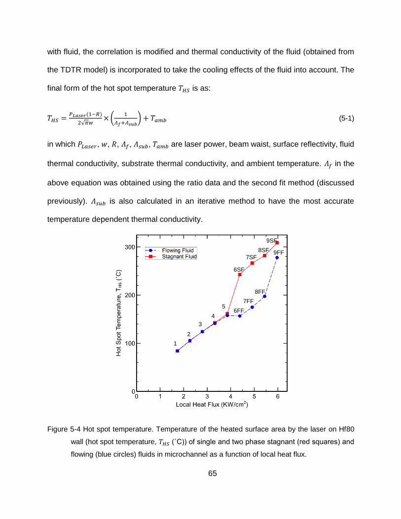
Figure 5-4 Hot spot temperature. Temperature of the heated surface area by the laser on
Hf80 wall (hot spot temperature, 𝑇𝐻𝑆 (˚C)) of single and two phase stagnant (red
squares) and flowing (blue circles) fluids in microchannel as a function of local heat
flux. ..................................................................................................................... 65
Figure 5-5 Pool and flow boiling curves by TDTR. Local HTC enhancement of single and
two phase stagnant (red squares) and flowing (blue circles) fluids in microchannel
as a function of hot spot temperature. ................................................................ 69
Figure 5-6 Transient TDTR measurement data. In phase (a) and out of phase (b)
components of the transient TDTR signal for subcooled flow boiling of water in
microchannel and their ratio (c). ......................................................................... 71
Figure 5-7 Ebullition cycle events of a single bubble. Time frame (a) and the ratio (b) of
life span events of a single bubble in pool and flow boiling. ............................... 73
Figure 5-8 Calculated transient local HTC vs time in the cross flow microchannel by the
differential TDTR scheme. Six images on the top show screenshots of the recorded
video at the specified data points. Fluctuating bottom line indicates the fully-grown
status and peaks show the ONB status .............................................................. 75
Figure A-1 TDTR in-phase (a), out-of-phase (b), and ratio (c) data as a function of time
for flowing water in a microchannel using a Ti-coated FS glass window. ........... 79
Figure A-2 TDTR ratio data (black symbols) and model predictions (red lines) as a
function of pump-probe delay-time for a NbV-coated FS glass window in thermal
contact with non-flowing (stagnant) water or air in the microchannel (𝑓mod = 962
kHz, 𝑃𝑃𝑢𝑚𝑝 ≈ 10.5 mW, 𝑃𝑃𝑟𝑜𝑏𝑒 ≈ 2.8 mW, 𝑤𝑃𝑢𝑚𝑝 = 8.7 μm, 𝑤𝑃𝑟𝑜𝑏𝑒 = 6.7 μm).
........................................................................................................................... 80
Figure A-3 TDTR ratio data (black symbols) and model predictions (red lines) as a
function of pump-probe delay-time for a Hf80-coated FS glass window in thermal
contact with non-flowing (stagnant) water or air in the microchannel (𝑓mod = 962
Page 16
xv
kHz, 𝑃𝑃𝑢𝑚𝑝 ≈ 10.5 mW, 𝑃𝑃𝑟𝑜𝑏𝑒 ≈ 2.8 mW, 𝑤𝑃𝑢𝑚𝑝 = 8.7 μm, 𝑤𝑃𝑟𝑜𝑏𝑒 = 6.7 μm).
........................................................................................................................... 81
Figure A-4 In-phase (circle symbols) and out-of-phase (square symbols) components of
measured TDTR voltage signal as a function of pump-probe offset ratio for a
Nb0.5V0.5 -coated FS substrate in thermal contact with stagnant air in the
microchannel. ..................................................................................................... 82
Figure A-5 Comparison between the measured (symbols) and model predicted (lines)
out-of-phase TDTR voltage signal (𝑉𝑜𝑢𝑡) as a function of pump-probe offset ratio
(∆𝑥/𝑤𝑝𝑢𝑚𝑝) for different glass substrates coated with a Nb0.5V0.5 thin-film alloy.
........................................................................................................................... 83
Figure A-6 In-phase (circle symbols) and out-of-phase (square symbols) components of
measured TDTR signal as a function of pump-probe offset ratio for a Nb0.5V0.5 -
coated FS substrate in thermal contact with stagnant (open symbols) and flowing
(closed symbols) water in the microchannel. ...................................................... 84
Figure A-7 Thermal conductivity (a) and volumetric heat capacity (b) of the fluid using two
methods, variable Λw and constant Cw (open markers) and variable Λw and Cw
(filled markers) for both stagnant (red squares) and flowing (blue circles) fluids. 85
Page 17
xvi
LIST OF TABLES
Table 2-1 Characteristic heat transfer coefficients (h) for different “micro-scale”
cooling methods ............................................................................................................ 10
Table 2-2 Typical resolutions for a range of nanoscale-relevant thermal
measurement methods [67] ........................................................................................... 13
Page 18
xvii
LIST OF ACRONYMS, ABBREVIATIONS, AND SYMBOLS
𝐴 = area of pump-laser hot-spot
C𝑝 = volumetric heat capacity
𝒞 = constant
𝐷ℎ = hydraulic diameter
𝐷𝑡ℎ = thermal diffusivity
𝑒𝑡ℎ = thermal effusivity
𝑓mod = modulation frequency
𝐺 = interfacial thermal conductance
𝐺 = mass flux
H = microchannel height
ℎ = heat transfer coefficient (HTC)
ℎ0 = local HTC for a stagnant fluid
ℎ↑ = local HTC enhancement (↑) due to forced convection
𝐿 = microchannel length
𝐿𝑐 = characteristic length-scale for heat transfer
ℓ𝑡ℎ = thermal penetration depth
Nu = Nusselt number
Nu0 = local Nu for a stagnant fluid
Nu↑ = local Nu enhancement (↑) due to forced convection
Pr = Prandtl number
Page 19
xviii
�̃�laser = laser power converted into heat
𝑞 = heat flux
𝑞CHF = critical heat flux (CHF)
𝑅 = reflectance of the metal
Re𝐷 = Reynolds number based on hydraulic diameter =
𝑡𝑐 = characteristic time-scale for heat transfer
𝑇f = fluid temperature
𝑇f∞ = fluid temperature at the microchannel inlet
𝑇S = surface/wall temperature
𝑇HS = hot spot temperature
𝑉𝑖𝑛 = in-phase TDTR voltage
𝑉𝑜𝑢𝑡 = out-of-phase TDTR voltage
𝑉𝑖𝑛
𝑉𝑜𝑢𝑡 = TDTR voltage ratio
v⃗ avg = average fluid velocity
v⃗ g = group velocity of TDTR thermal waves
v⃗ ℓ𝑡ℎ = fluid velocity at a perpendicular depth ℓ𝑡ℎ from the hot-spot
v⃗ max = maximum fluid velocity in the center of the microchannel
𝑥 = flow direction, distance from the microchannel inlet
W = microchannel width
𝑤 = beam waist, 1/𝑒2 radius of the focused pump laser
𝑧 = perpendicular distance from the metal wall into the channel
Page 20
xix
Greek symbols
𝛿ℎ = thickness of the hydrodynamic boundary layer
𝛿𝑡ℎ = thickness of the thermal boundary layer
Δ𝑇 = temperature difference between the fluid and metal wall/surface
Δ𝑇𝐴𝐶 = amplitude of the temperature oscillations in metal due to 𝐴𝐶 pump heating
Δ𝑥 = pump-probe offset
Δ𝑥/𝑤 = offset ratio
𝜇∞ = dynamic viscosity of the fluid at the microchannel inlet
𝜇tBL = dynamic viscosity of the fluid in the thermal BL
𝜈 = kinematic viscosity
𝜔 = angular heating frequency
𝜏𝑑 = pump-probe time-delay
Λ = thermal conductivity
Acronyms
BL = boundary layer
fs = femtosecond
FS = fused silica
ktg = kinetic theory of gases
HTC = heat transfer coefficient
𝑅𝑂𝐼 = region of interest
Page 21
1
CHAPTER 1: INTRODUCTION
1.1 Background and motivation
1.1.1 Microscale high heat flux devices
For decades, there has been great interest among industries in scaling down and
shrinking their products’ size due to different reasons such as less material, weight, and
energy usage, smaller size, easier transportation and better portability, and final cost and
market desire. For example, the semiconductor and microelectronics industry has
benefited from continuous miniaturization evolution and power increase over the past four
decades to reduce room-sized Mainframe computers to million times faster laptops or
pocket-size cellphones. This evolution which has led to a new class of machines every 5-
10 years (shown in Figure 1-1(a)) [1], has been enabled by shrinking of transistors as the
fundamental building block down to 10-100 nm dimensions and placing 10-100 millions
of them on a single chip or an Integrated Circuit (IC) in the recent years. This is ruled as
Moore's law and states that the number of transistors on a microprocessor chip will double
every two years as indicated in Figure 1-1(b).
We would be lucky if the increased functional density and reduced size and cost
were the only consequences. However, overheating was a throwback to the
miniaturization which began when the feature size reached the 90 nm limit and below in
the early 2000s. The solution to this was to cap the processors’ clock speed as it’s shown
Page 22
2
by the blue plateau area in the Figure 1-1(b) while increasing the number of chips by
redesigned multi-core processors [1].
“High Heat Flux” (HHF) situation, which means relatively large amount of heat
loads distributed or imposed over smaller areas [2], can be seen not only in
microelectronics but in many of today’s devices and technologies such as diode lasers,
data centers, energy production and storage systems. Figure 1-1(b) outlines this growing
challenge faced by the microelectronics industry for the next generations of devices [1],
where, for example, the heat fluxes within the next decade are expected to surpass 3
KW/mm2 which is nearly 50 times greater than the heat flux radiated by the Sun [3].
The heat dissipation in an IC is highly local with some high temperature and high
Figure 1-1 (a) Computer miniaturization evolution [1]. (b) Number of transistors per chip, Moore’s
law (black-line), microprocessor clock speeds (blue circles), hot-spot heat fluxes
calculated via the transistor and clock-speed trends for a processor die area of 500 mm2,
DARPA’s goal of 20 pJ per (fl)op, and (fl)op efficiencies of 90% and 98%.
1970 1980 1990 2000 2010 2020
108
104
102
106
1
Year
106
1010
He
at F
lux
Tre
nd
(M
W/m
2)
1
108
104
Moore’s LawTransistors per Chip
(a)
Heat FluxTrend
(c)
1010
(MHz)Clock speeds
(b)102
90% 98%
@nature
(a) (b)
Page 23
3
heat flux points on the circuit which are known as “hot spots”. The greatest thermal
challenges in microelectronics is in the packaging of processors not only due to the largest
overall power dissipation, but because the hot spots [4]. According to the 2015
Technology Roadmap for Semiconductors [5], both average and local power densities
will increase in the future designs. Performance and reliability of thermal solutions will be
limited by transient hot spot thermal management even when the total and average power
meets the design specification and requirements.
1.1.2 Thermal transport at nano-interfaces
Development of nano-devices in microelectronics, biomedical, or energy
applications brings concerns about removal of the dissipated heat and thermal
management at interfaces between nano-layers and other materials or mediums [6,7].
Since nano-structures or nano-devices have relatively less bulk material, thermal
transport is dominated at their interfaces [7]. To understand this behavior let’s take a
closer look at the thermal transport at interfaces. Figure 1-2 shows heat flow (𝑞) from the
box A (left) to the box B (right) and temperature distribution along the heat flow direction
for three cases. In the first one there is an air gap at the interface due to surface roughness
and imperfect contact. These air gaps and rough surfaces create a resistance to the heat
flow which is called Thermal Contact Resistance (𝑅𝑐) and it causes a temperature drop
of ∆𝑇𝑐 = 𝑇𝐴 − 𝑇𝐵 from the surface A to the surface B across the interface. Contact
resistance is macroscopic and important to bulk surfaces.
In Figure 1-2 (b) the contact surfaces of A and B are perfect with no roughness
Page 24
4
Figure 1-2 Heat flow across a (a) common bulk interface, (b) perfect and ideal bulk interface, and
(c) nano-interface and temperature drop at the interface due to (a) contact resistance, (b)
boundary resistance, and (c) nano-structure boundary resistance
and air gap between. Unlike the common sense of no resistance and temperature drop
at this interface there is a resistance due to different acoustic (vibrational and electronic)
properties of materials and surfaces of A and B which is called Thermal Boundary
Resistance (𝑅𝑏). It happens when an energy carrier (phonon or electron) scatters at
interface while trying to crossover the interface. Boundary resistance is microscopic,
present even at ideal contacts, and important to nano-structures and small scale devices.
As it’s illustrated in Figure 1-2 (c) when the box A is converted to a thin layer instead all
the heat should flow through the thin layer and since there is less bulk material and
surfaces the temperature drop of ∆𝑇𝑏 is more than (b).
Thermal boundary resistance (or inversely interfacial thermal conductance (𝐺))
relates the heat flow 𝑞 crossing the planar interface to the local temperature drop ∆𝑇𝑏 at
the interface between two sides by this equation [8]:
𝑞 = ∆T 𝑅𝑏 = 𝐺∆T⁄ (1-1)
Thermal interface conductance which has the 𝑊/𝑚2. 𝐾 unit, has a limited range at
room temperature for balk materials interface compared to the other thermal properties
A, ΛA B, Λ
B
q
TA
TB
A, ΛA B, Λ
B
q T
A
TB
q T
A
TB
(a) (b) (c)
Page 25
5
based on the interface composition at a molecular layer level [9] and is usually measured
between 10 and 100 𝑀𝑊/𝑚2𝐾 [7,10–13] for practical materials and applications. For the
physical meaning purpose, 𝐺 can be interpreted as an equivalent thermal impedance or
an equivalent thickness (𝑑) of a dielectric layer by relating them to the thermal conductivity
of dielectric (𝐺 = 𝛬 𝑑⁄ ). For example, an interface with a typical conductance of 𝐺 =
107𝑊/𝑚2𝐾 (or 𝑅𝑏 = 10−7𝑚2𝐾/𝑊) is equivalent to the thermal impedance of 140 nm of
SiO2 or 15 µm of Si.
As we know one or more of heat carriers (phonon, electron, or photon) and/or fluid
particles (atoms or molecules) are present and dominant in any heat transport process
depending on the material type, phase, and mode of heat transfer. The upper limit for
interfacial thermal conductance of bulk materials belongs to high-conductivity-metals
interfaces such as Al/Cu with electrons as dominant energy exchange carriers and the
lower limit of 𝐺 is at interfaces with highly mismatched phonon modes such as Bi/H-
diamond [11].
Heat carriers or fluid particles have interactions with each other at interfaces such
as phonon-phonon, phonon-electron or phonon-boundary scattering due to the
differences in electronic and vibrational properties in different materials. When an energy
carrier attempts to traverse the interface, it will scatter at the interface which makes heat
transport at interfaces more difficult to predict.
In Figure 1-3 (b) a typical transistor with micro-size substrate and nano-size device
layer is shown. In the left side (Figure 1-3 (a)) mean free paths of phonons in some
common substrate materials are plotted as a function of temperature. It has been
observed that length scale of the substrate or device determines heat transport
Page 26
6
mechanism at any given temperature. For example, at room temperature heat transports
diffusively within Si and SiC for dimensions above ≅ 550 𝑛𝑚 and 1.1 µm respectively and
ballistically or quasi-ballistically below those limits. Fourier diffusion law for macroscopic
sizes fails when characteristic length of the device or the system is comparable to the
mean free path of the heat carrier or when the time scale of the physical system is smaller
than the relaxation time of the heat carriers.
All the above-mentioned issues imply that low thermal resistance or high
conductance at interfaces is desirable for very high heat flux and dissipation applications.
As expected by the International Technology Roadmap for Semiconductors this is vital to
the development of microelectronic semiconductor devices where an 8 nm feature size
device is projected to generate up to 100 kW/cm2 and would need efficient heat
dissipation of an anticipated die level heat flux of 1 kW/cm2 which is an order of magnitude
higher than current devices [14]. This means that interfaces are critical at the nanoscale.
Figure 1-3 (a) Temperature dependence of the mean free paths of phonons in a variety of
common substrate materials. (b) Typical transistor with nano-size device layer
(a) (b)
@nature
Page 27
7
1.2 Approach and outline
Microscale liquid cooling is a promising cooling method for high heat flux systems.
Different forms of liquid cooling systems as spray cooling, jet impingement, immersion,
heat pipes, mini and microchannels have been developed during the last two decades.
Microchannels have been of particular interest for practical microscale cooling of HHF
systems. Microchannel is used in this dissertation to study heat transport at its nano-size
wall interface with liquid coolant using an optical and non-contact high resolution
technique called Time-Domain Thermo-Reflectance (TDTR).
In the next chapter theories and literatures related to microscale cooling of HHF
devices and TDTR method will be provided. Details about the experimental setup of
sample stage, microchannel, and TDTR and the measurement methodology will be
discussed in chapter CHAPTER 3:.
For proof of principle, single-phase water in rectangular microchannels and
corresponding methodology for HTC analysis to decipher the thermo-fluid transport inside
and outside the thermal BL will be studied in chapter CHAPTER 4:. This work also builds
on past TDTR studies of droplet impingement and evaporation and facilitates later
thermo-physical studies of multi-phase heat and mass transport in chapter CHAPTER 5:.
Summary and future direction will be concluded in chapter CHAPTER 6:.
Page 28
8
CHAPTER 2: THEORY AND LITERATURE
2.1 Introduction
Temperature control is a critical regulatory process in a wide variety of systems.
Without it, sustainable operation isn’t possible in arguably everything from the
functionality of biological organisms [15] to the reliability of electronic [1,16], photonic [17],
and electro-chemical devices [18], to high-speed transportation [19] and materials
manufacturing [20]. For today’s technologies, there seems to be a ubiquitous trend
towards increasingly smaller, more capable, and higher energy or power density devices.
Subsequently, without concurrent advances in energy efficiencies, these smaller and/or
more powerful devices require improved thermal management systems to maintain their
temperatures within operational limits at higher heat flux conditions.
This work revisits hot-spot cooling in microchannels, focusing on the validation of
our optical pump-probe method to characterize large, gradient-driven heat and mass
transport.
2.2 Microscale cooling of high heat flux devices
For high heat flux thermal management, microscale cooling with liquids has
become a promising alternative to traditional air cooling due to the liquids’ larger heat
capacity, thermal conductivity, and intrinsic ability to dissipate large amounts of thermal
energy (heat) – or regulate fluctuations in surface temperature – via liquid-vapor (latent
heat) phase transformations. In result, there has been significant interest by academia
and industry on convective and phase-change heat transfer at the micro- and nano-scale,
Page 29
9
where hundreds of papers have been published on related liquid cooling processes
including (but not limited to): single-phase flow [21], multi-phase flow [22,23], flow boiling
[24], pool boiling [25,26], spray cooling [27,28], heat pipes [29,30], thermosyphons [31],
microdroplet evaporation [32], single-phase jet impingement cooling [33,34], and micro-
jet impingement boiling [35,36].
The Holy Grail for all these liquid cooling techniques is an accurate, predictive
understanding of the heat transfer coefficient (h or HTC). In general, the cooling efficiency
of any heat removal process is encapsulated by the HTC, which is a proportionality
constant that couples the heat flux (q) to the temperature difference (∆T) that drives the
heat flow. The magnitude of the HTC is dictated by several factors, including the velocity
distribution of flow-field, the thermo-fluid properties of the coolant, and surface
characteristics of the device (e.g., geometry, micro-structure, temperature, and
chemistry).
Table 2-1 summarizes the range in h for a variety of different cooling methods. As
shown, techniques based on phase-change heat transfer (e.g., boiling and evaporation)
have, most commonly, improved HTCs relative to their single-phase (e.g., non-boiling)
counterparts; however, these multi-phase cooling methods also suffer from the reality that
the added materials phase coincides with a much higher propensity to induce a critical or
unstable “cooling regime”. In which case, the cooling performance of a multi-phase
system operating in a so-called “unstable cooling regime” typically coincides with an order
of magnitude reduction in the HTC. A well-known example is the onset of the critical heat
flux (CHF) during nucleate pool boiling, where at CHF (and at wall superheats beyond the
CHF) the HTC can decrease by several orders of magnitude [37]. Another well-known
Page 30
10
example is the onset of wall-dryout during thin-film evaporation and nucleate flow boiling
[38–40].
Table 2-1 Characteristic heat transfer coefficients (h) for different “micro-scale” cooling methods
Cooling
method
Microchannels
(single-phase)
Microchannels
(boiling)
Jet impingement
(single-phase)
Jet impingement
(boiling)
Fluid Water Refrigerant Water Refrigerant Water Refrigerant Air Water Refrigerant
𝒉 (kW/m2∙K)
[Ref]
10 – 500
[41]
1 – 30
[42]
20 – 200
[43,44]
2 – 100
[45]
30 – 320
[46]
40 – 400
[46]
5 – 400
[47]
200 – 1000
[48]
50 – 120
[46]
The optimal cooling method is also dictated by several other factors such as
system size, cost of operation, and desired control scheme (i.e., active or passive). For
instance, spray cooling with water is currently the most effective process for dissipating
large thermal loads (i.e., heat fluxes ~10 MW/m2) from the surfaces of moderately sized
systems (e.g., surface areas < 0.5 m2) [40,49], whereas jet impingement boiling is the
optimal method for dissipating ultra-high heat fluxes (e.g., heat fluxes in the range of 0.5
– 20 MW/m2) from sub-mm2 sized hot-spots [35,50].
To date, the largest HTCs are observed with techniques based on jet impingement
boiling. Interestingly, for sub-cooled jet impingement boiling, the HTC at the edge of the
stagnation zone is found to decrease with increasing wall temperature until the onset of
nucleate boiling [48], supporting that the local maximum in the HTC is at the edge of the
stagnation zone and coincides with the cooling region where no phase-change and only
sensible heat transfer takes place [51]. Within the stagnation zone the thickness of the
thermal boundary layer (BL) is at a minimum and the acceleration of flow-field is at a
Page 31
11
maximum. Recently, Mitsutake et al. [52] have shown that heat fluxes within 48% of the
theoretical maximum can be obtained with jet impingement cooling. For reference,
typically two-phase cooling methods achieve CHF values that are less than 10% of this
theoretical limit (i.e., 𝑞CHF < 0.1 𝑞maxktg
, where 𝑞maxktg
is the maximum evaporative heat flux
predicted by the kinetic theory of gases) [53]. Another interesting finding for spray or jet
impingement boiling is that the addition of non-condensable gases (NCGs) to coolant can
increase the overall HTC [46,54]. This is a rather counter intuitive result because the
addition of NCGs should effectively decrease the heat capacity and thermal conductivity
of the coolant and thereby reduce the sensible heat contributions to the HTC.
The importance of the sensible heat contributions and NCGs to the HTC in two-
phase cooling is not new. However, most studies correlate the boiling and evaporation
performance to only the latent heat contributions and mixed results are reported for NCGs
[55,56]. In support, are the past spray cooling studies by Kim and Kiger [] and the very
recent pool boiling studies by Jaikumar and Kandilkar [54,57]. For the latter, the studies
by Jaikumar and Kandikar showed that the record HTC values of ℎ ≈ 800 kW/m2∙K were
observed with specific micro-pillar surfaces that presumably optimized the sensible
cooling by minimizing nucleation and maximizing liquid convection at the base of the
micro-pillars. We hypothesize that this sensible cooling effect at the base of the micro-
pillars is directly correlated with the increased HTC observed within the stagnation zone
for jet impingement boiling. In both cases, for example, the fluid flow-field presumably
induces a suppression of the thickness of the thermal BL, ultimately increasing the HTC
for a prescribed heat flux.
Page 32
12
These results (among others) warrant the need to better decipher the relative
significance between the different cooling mechanisms that dictate phase-change heat
and mass transfer phenomena, especially at the micro- and nano-scale and at time-
scales fast enough to render transient changes in the hydrodynamic and thermal
boundary layers [58–61]. In micro-domains, multi-phase flow boiling and heat transfer is
attributed to four key mechanisms: microlayer evaporation, interline evaporation,
transient conduction, and micro-convection [59]. For reference, the sensible heat
contributions discussed previously are effectively regulated by the rate at which the
coolant can be heated (i.e., the rates of micro-scale conduction and convection within the
thermal BL). To accomplish this level of thermo-physical characterization, new
synchronized thermo-fluid diagnostics are needed that can combine high-fidelity
temperature and flow-field measurements at spatial- and temporal-resolutions of < 5 μm
and < 200 μs, respectively [60].
2.3 Time-Domain Thermo-Reflectance (TDTR)
In this section, the optical diagnostic method called Time Domain
Thermoreflectance (TDTR) and the approach used in the Interfacial Transport Lab at UCF
to characterize the local HTC in the thermal BL of flowing fluids will be introduced. TDTR
is a well-established optical technique used by the thermal science community to
characterize micro and nanoscale heat transport (e.g., most frequently the thermal
conductivity and interfacial thermal conductance).
Interfacial thermal conductance is usually measured by optical pomp-probe
methods such as Time-Domain Thermo-Reflectance (TDTR), 3-ω, or Picosecond
Page 33
13
Transient Absorption methods or estimated by Acoustic or Diffusive Mismatch Models
(AMM or DMM) or Molecular Dynamics Simulation (MDS). Here, TDTR technique which
is setup in the Interfacial Transport Lab at UCF will be used in this study. TDTR is a
technique that has acceptable resolution in all three criteria of space, time, and
temperature. Table 2-2 shows typical resolutions for a range of nanoscale-relevant
thermal measurement methods with highlighted values for the thermoreflectance (TDTR)
method.
The TDTR technique uses two concentrically focused pump and probe laser
beams to heat (with the pump) and then measure (with the probe) the temporal changes
in heat transport in a sample [62–64]. The recently developed anisotropic version of TDTR
will be also employed in this work, where nonconcentric beams are used to heat (pump)
and measure (probe) the anisotropic thermal transport properties by spatially offsetting
pump and probe beams in small increments [65,66].
Table 2-2 Typical resolutions for a range of nanoscale-relevant thermal measurement methods [67]
Method Spatial
resolution (μm)
Temperature
resolution (K)
Response
time (μs)
Near-field scanning optical microscopy 10−2
10−1
10
Transmission electron microscopy 10−2
10−1
10
Thermoreflectance 10−1
10−2
10−1
Fluorescence 10−1
10−2
10
Scanning thermal microscopy 10−1
10−1
102
Optical interferometry 1 10−5
10−3
Raman 1 10−1
106
Infrared thermography 10 10−1
10
Liquid crystals 10 10−1
102
Thermocouple 102 10
−1 10
Page 34
14
The TDTR measurement principle is based on measuring rate of heat removal
from a metal thin-film by its surroundings. For example, in this study, the cooling of a Ti
thin-film (≈64 nm in thickness) by flowing water (top) and the FS substrate (bottom). In
regards to the pump-probe aspect of the TDTR method, consider a focused pulse train of
laser light (i.e., the pump beam) that heats the surface of the metal. Now, each fs pulse
of the focused pump beam induces a local temperature jump (∆𝑇) in the metal over an
area, 𝐴 ≈ 𝜋𝑤2. Then, after each fs heating event, the metal dissipates heat to its
surroundings. Thus, the metal thin-film serves as both a heater and a thermometer, where
the rate of heating is nearly instantaneous (e.g., fs heating) and the rate of cooling is
dictated by the overall thermal conductance (or thermal effusivity - 𝑒𝑡ℎ) of the
surroundings. For example, the cooling rate becomes more rapid by increasing either the
thermal conductivity (Λ) or heat capacity (C𝑝) of the surroundings.
The thermometry aspect of TDTR is accomplished by the probe beam. For
example, a short time-delay after each pump heating event (e.g., 𝛿𝑡 = 𝜏𝑑), the probe
beam (also, a focused, pulse train of laser light) “probes” the change in temperature of
the metal. The probe beam actually “probes” the change in reflectivity of the metal, which
is coupled to the metal’s local temperature by its thermoreflectance coefficient (𝑑𝑅/𝑑𝑇).
Hence, the name of the TDTR technique: time-domain thermoreflectance.
TDTR measured data should be compared to a heat transfer model of the sample
in order to analyze the result. The model is used here has columns of heat conductivity,
volumetric heat capacity, and thickness of all the material layers and interfaces between
them. Unknown thermal parameters are determined by minimizing the difference between
measured data and model [62].
Page 35
15
CHAPTER 3: EXPERIMENTAL SETUP AND METHODOLOGY
This chapter is divided into three sections. In the first two sections, details about
the sample stage and flow loop including microchannel fabrication, samples, and video
imaging and about TDTR optical and data acquisition setup are explained. The last
section discusses the method used for data reduction and uncertainty analysis.
3.1 Sample stage and flow loop
Figure 3-1 provides a schematic overview of the microchannel sample stage and
flow loop of the experimental setup. It shows the flow-loop methodology based on the use
of a custom syringe pump design that incorporates fluid pumping via two identical
syringes (36 mm, inner diameter) with bonded plunger ends. All reported experiments are
for fluid flow in the indicated flow direction; however, the flow direction can be easily
reversed and reversed flow has no noticeable effect for local measurements in the center
of the microchannel (data will be presented later). This is expected since the experiment
is done at atmospheric pressure and flow direction is horizontal so there is no gravity
effect on the flow direction and the data. The current setup facilitates volumetric flow rates
ranging from 0.2 𝑚𝐿/𝑚𝑖𝑛 to 55 𝑚𝐿/𝑚𝑖𝑛, which corresponds to ranges in average flow
velocity (v⃗ avg), mass flux (𝐺), and Reynolds number (Re𝐷) with our microchannel setup of
0.01 ≲ v⃗ avg ≲ 3.8 m/s, 13.9 ≲ 𝐺 ≲ 3808 kg/m2/s, and 7 ≲ Re𝐷 ≲ 2031, respectively. Most
of reported experiments are based on a pumping rate of 50 mL/min, corresponding to
Re𝐷 ≈ 1850 using atmospheric pressure and room temperature water-inlet properties for
the fluid, unless otherwise mentioned. For precise alignment, the microchannel sample
Page 36
16
Figure 3-1 Sample stage and flow loop of the experiment.
stage is mounted on 6-axis stage, providing three (3)-translational and three (3)-rotational
axes (or degrees-of-freedom) for translation and alignment.
3.1.1 Microchannel
Figure 3-2 provides an expanded view of the construction and design of the
microchannel sample stage. As shown, the microchannel consists of three primary
pieces: an Acrylic polymer substrate (1 inch, diameter; 1/8 inch, thick), a micro-patterned
Polydimethyl-siloxane (PDMS) seal (≈ 400 μm, thick), and a metal-coated fused silica
(FS) glass window (1 inch, diameter; 1/16 inch, thick). The microchannel is constructed
by pressure sealing the acrylic substrate to the metal-coated FS window. The
microchannel geometry (or cutout in the PDMS seal) is fabricated by laser ablation
processing of the microchannel negative in an Acrylic piece and then molding the PDMS
mixture in the negative by heat curing at 130 ˚C for 25 minutes. Laser ablation patterning
Page 37
17
is also used to make the fluid inlet- and outlet-ports (≈ 1 mm, diameter) in the acrylic
substrate. After pressure sealing, the microchannel dimensions are verified using the
camera imaging setup shown in Figure 3-1. No leaking of the PDMS seal or flow-loop is
observed for the maximum allowable flow rates of 55 mL/min. however finding the right
sealing pressure in a way that there is no leaking and no flow blockage or microchannel
dimension change due to the PDMS flexibility and softness is a tedious and difficult task
which achieved by try and error. The microchannel length, width, and height dimensions
are 𝐿 ≈ 15 mm, W ≈ 600 μm, and H ≈ 400 μm, respectively. These channel dimensions
correspond to a hydraulic diameter of 𝐷ℎ ≈ 480 μm by this equation:
𝐷ℎ =2𝐻𝑊
𝐻+𝑊= 480 µ𝑚 (3-1)
Figure 3-2 Expanded view of the microchannel construction
Pump
Probe
Acrylic substrate
Fused Silica window
Metal thin-film
PDMS
seal
𝒚
𝒛 𝒙
𝐖 𝐇
Page 38
18
3.1.2 Samples
Th samples in the experiments conducted in this research work are 1 inch,
diameter and 1/16 inch thick fused silica (FS) windows coated with different 50-100 nm
metals or alloys. Metals or alloys with large thermoreflectance coefficients are ideal for
TDTR. Aluminum (Al) is widely used in thermoreflectance experiments because of its
broad applications in microelectronics, superior thermal properties, and relatively high
thermoreflectance coefficient (𝑑𝑅 𝑑𝑇⁄ ). However, because of the Al corrosion in contact
with water and heat flow (which will be discussed later) it is not a reliable and good choice
as a transducer for solid-liquid interfaces. So, other metals such as Titanium (Ti) and
alloys such as NbV or Hf80 were tested and investigated.
Ti shows better stability in contact with water and has variety of applications in high
heat flux cooling systems. The NbV alloy used by Feser and Cahill is also one such thin-
film alternative to Al [66]. Moreover, of importance to the water flow studies in this
dissertation, NbV alloys have corrosion resistance properties that are superior to Ti. In
addition to Ti and NbV, a complex metal alloy consisting of Hf, Gd, and HyMu80 alloy
(which we call Hf80 due to its highest Hf content) is also used. This Hf80 metal alloy not
only has a low thermal conductivity (e.g., Λ ≅ 5.6 W/m∙K), but it is incredibly robust,
facilitating later TDTR studies of flow boiling and jet-impingement with extreme hot-spot
heat fluxes. All these thin-films are deposited on the FS substrates by physical vapor
deposition techniques.
Page 39
19
3.1.3 Imaging
Imaging using high speed cameras is an essential part of any micro and nanoscale
flow and heat transfer studies. In the current heat transfer investigations in the
microchannel using TDTR the camera setup facilitates flow visualization and alignment
of the pump-probe lasers in the microchannel. Note that there are two cameras, the main
one in the backside of the stage mainly used for flow visualization which we may refer as
the back camera and another one in stage front for TDTR beams alignment which is
referred as the front camera. The back camera is a Flea3 USB 3 camera with 150 FPS
at 1280 x 1024 resolution which gives 6 ms or less (1 ms at smaller ROI sizes) time
resolution. Since the TDTR laser lights have lots of shining and scattering reflections on
the microchannel which makes the flow in the channel invisible, a short-pass filter is used
before the back camera’s sensor after TDTR alignment is done.
3.2 TDTR setup
Facilities for optical pump-probe diagnostic techniques are not available
commercially as a package and are usually built in-house in labs based on applications,
desired measurement parameters, and the budget. They consist of laser and optical
elements on the optical table and data acquisition and electronic apparatus. Figure 3-3
shows our base in-house TDTR optical setup (a) and data acquisition and analysis (b)
system, using the two-tint methodology [63] which will be discussed in the next two
sections.
Page 40
20
Figure 3-3 TDTR optical setup (a) and data acquisition and analysis system (b)
3.2.1 Optics
In our TDTR setup, the laser source is a Coherent Chameleon femtosecond
Ti:Sapphire laser (pulse frequency: 80.1 MHz, pulse width: 140 fs, central wavelength:
787 nm). The Chameleon laser output is split into two laser beams (pump and probe).
The pump beam is frequency modulated at either 𝑓mod = 9.81 MHz, 976 kHz, or 962 kHz
using an Electro-Optic Modulator (EOM). The two-tint system is used to help filter
(remove) pump laser light on the differential photodiode (PD) detector. After the EOM, the
pump beam is reflected (down and back) using an Au retroreflector on a mechanical delay
stage. After the other optics indicated in Figure 3-3 (a), the pump and probe beams are
concentrically focused onto the metal thin-film on the sample using a 20× Mitutoyo, infinity
corrected, long-working-distance microscope objective.
The spatial variation in the pump path length by the delay stage is equivalent to a
temporal time-delay (𝜏𝑑) between each focused pump and probe pulse on the
Page 41
21
metal/sample. TDTR setup in the Interfacial Transport Lab achieves pump-probe time-
delays of -120 ps < 𝜏𝑑 < 3.3 ns. The focused beams waists of pump and probe beams
on the metal/sample (𝑤) are most frequently ≈9.5 µm and ≈8 µm, respectively. The
incident pump and probe laser powers on the sample are adjusted to maximize the
measurement signal (for a minimum amount of probe power) while also ensuring that total
dc temperature rise/heating of the pump-induced hot-spot is no more than 60 K (typically,
< 11 mW and < 5 mW for the pump and probe, respectively).
3.2.2 Data acquisition
A differential PD detector used to measure the probe’s thermoreflectance signal of
the sample as a function of 𝜏𝑑, where again this thermoreflectance signal is induced via
the frequency-modulated heating by the pump beam. The time-domain voltage output of
the detector is measured by a lock-in amplifier at a reference frequency equal to 𝑓mod,
using triple-shielded RF coax-cables and a resonant band-pass filter between the
detector and the lock-in amplifier (see Figure 3-3 (b)). The lock-in amplifier extracts the
detector voltage signal into in-phase (𝑉𝑖𝑛) and out-of-phase (𝑉𝑜𝑢𝑡) voltage components in
the frequency-domain. These voltages as a function of pump-probe delay (𝜏𝑑) are then
compared to the predictions of a TDTR thermal transport model to extract the thermal
properties of the sample.
We use, as most commonly done by others, the in-phase to out-of-phase voltage
ratio (𝑉𝑖𝑛/𝑉𝑜𝑢𝑡) to correlate the time-domain changes in the surface reflectivity to the
thermal transport properties of the sample [62,64,68]. In short, the TDTR voltage ratio
(𝑉𝑖𝑛/𝑉𝑜𝑢𝑡) is the key measurement parameter for characterizing the thermal transport
Page 42
22
properties of a sample. This work shows how measurements of 𝑉𝑖𝑛/𝑉𝑜𝑢𝑡 can be used to
extract the local HTC of flowing and stagnant fluids.
3.3 Errors and uncertainty
The phase of the lock-in amplifier, modulation frequency, film thickness, the beam
spot size, and the laser intensity and resulting temperature rise are common sources of
uncertainties in TDTR experiment [69,70]. Uncertainties related to the phase and
temperature rise are relatively small for modulation frequencies larger than 1MHz and dc
heating less than 20 K. The error between the data and the model is minimized by
adjusting the model parameters. Error bars associated with the standard deviation of the
average values from repeated measurements at the same spot are shown in the plots.
Page 43
23
CHAPTER 4: SINGLE PHASE HEAT TRANSPORT USING TDTR
4.1 Baseline TDTR measurements
The TDTR method does not require a calibration. Rather, the measurement
accuracy is validated by reproducing thermal property data of known materials systems
using no free parameters in the TDTR thermal transport model. In this regard, the TDTR
method is not limited by its measurement resolution; rather, TDTR is limited by its
measurement precision (i.e., reproducibility of a measurement). In principle, the technique
can measure a local, transient HTC within the range of 100 kW/m2/K ≲ ℎ ≲ 500 MW/m2/K
over spatial measurement areas within 10 – 2500 μm2 and at a minimum temporal time-
scale of ≈100 μs. This predicted range of TDTR measurement-space for the HTC is
based on (i) a practical range in thermal conductivities that can be measured with the
TDTR (e.g., 0.01 ≲ Λ ≲ 3000 W/m/K), (ii) a practical range in the footprint/measurement
area for the focused pump-probe lasers (e.g., 10 ≲ 𝑤2 ≲ 2500 μm2), and (iii) the minimum
time-constant setting (𝜏m) of a MHz bandwidth lock-in amplifier (i.e., 𝜏m = 100 μs). We
note that this discussion did not consider the length-scale that the HTC is probed within
the thermal BL. This topic is addressed in section 4.2. It should also be pointed out that
the precision of HTC measurements in this setup (discussed later) were observed to be
within δℎ ≈ ± 100 kW/m2/K.
In order to verify the experimental setup and confirm the thermal properties of the
metal thin-film heater, water, FS substrate, and other parameters in the TDTR model, full
Page 44
24
time-delay TDTR scans have been conducted and repeated with both air and water in
contact with the Al and Ti coated FS substrates.
4.1.1 Aluminum-water interface
Aluminum (Al) is widely used in thermoreflectance experiments because of its
broad applications in microelectronics, superior thermal properties, and relatively high
thermoreflectance coefficient. A preliminary front-side TDTR experiment was performed
with the experimental details mentioned previously using ~66 nm of Al on a FS substrate
using literature thermal properties [58]. The resulting data good (i.e., no free parameter)
fits between the model and measured data other than the interfacial conductance (G)
between the Al layer and the FS substrate (GAl-FS =150 MW/m2-K) which is within the
expected range measured by others and validates our experimental methodology and
TDTR setup.
For Al-water interface measurements in the microchannel the results are not
consistent and the ratio changes with time and from one spot to another. The reason for
this inconsistency is that when Al is in contact with water is corroded uniformly or locally
by water flow (flow-assisted corrosion) [71] and/or by increasing temperature of the Al or
water (temperature-assisted corrosion) [72]. Such corrosion effects commonly result in
pitting and deterioration of the Al surface (visible by the eye) and significant changes in
the Al thickness and reflectivity.
Page 45
25
4.1.2 Titanium-water interface
Ti-based thermal management solutions for high heat flux applications have been
developed in the recent years because of its preferable mechanical, and thermal
properties which includes higher strength to weight ratio, and closer thermal expansion
coefficient to silicon-based chips [73]. Furthermore, it does not erode and corrode in
flowing aqueous environments and shows more stability at higher temperatures in liquid
cooling applications.
Figure 4-1 TDTR ratio data (symbols) and model predictions (lines) as a function of pump-probe
delay-time for a Ti-coated FS glass window in thermal contact with non-flowing (stagnant)
water or air in the microchannel (𝑓mod = 962 kHz).
After validation of the experimental setup with Al sample, a ~64 nm Ti layer on a
1” FS substrate is selected as the base sample for the rest of the experiments. Figure 4-1
shows the predicted 𝑉𝑖𝑛/𝑉𝑜𝑢𝑡 ratio as a function of pump-probe delay (𝜏𝑑) with
comparisons to measured data for both air and non-flowing (stagnant) water in contact
with a Ti metal coated FS glass window. The model predictions (lines) are based on
literature thermal property data for the fluid (air or water), Ti thin-film, and FS glass
100 1000
Delay-time, d (ps)
0.5
1.0
1.5
2.0
TD
TR
ratio
,V
in/
Vo
ut
data
model
400020
Air
Water
𝑉 𝑖𝑛/𝑉
𝑜𝑢𝑡
Fused
Ti e.g., Air or Water(64 nm)
Silica
Sample of Interest
𝒙
𝒛
≈1 MHz
Pump Probe
Page 46
26
substrate. The TDTR experiments and modeling with an air-filled microchannel are used
to determine and validate the thermal properties of Ti and FS (which are also used and
verified repeatedly for all subsequent TDTR experiments). For example, the measured
thermal conductivity and volumetric heat capacity of Ti were 𝛬𝑇𝑖 = 20 𝑊 𝑚.𝐾⁄ and 𝐶𝑝𝑇𝑖 =
2.384 ×10⁶ 𝐽 𝑚3. 𝐾⁄ , respectively, which are in good agreement with literature data for Ti.
The schematic in Figure 4-1 corresponds to the materials and measurement
configuration, where the pump-probe beams pass through the FS glass substrate and
then heat the “backside” of the Ti thin-film. The data in Figure 5 shows that the magnitude
of 𝑉𝑖𝑛/𝑉𝑜𝑢𝑡 is larger for the more thermally conductive fluid – i.e. water (as opposed to air)
in the microchannel. Also, for these “backside” TDTR measurements, oscillations in
𝑉𝑖𝑛/𝑉𝑜𝑢𝑡 are observed (see, Figure 4-1) – presumably due to Brillouin backscattering in
the glass substrate [64]. We point out the oscillation peak at 100 ps because this study
uses 𝑉𝑖𝑛/𝑉𝑜𝑢𝑡 measured at a single delay time (i.e., 𝜏𝑑 ≈ 100 ps) to predict the HTC of
flowing fluids. Thus, our measured fluid thermal conductivities and corresponding HTC
predictions will be slightly overestimated (e.g., 5-20 %, with and without fluid flow) based
on 𝑉𝑖𝑛/𝑉𝑜𝑢𝑡 measured at solely 𝜏𝑑 ≈ 100 ps. Conversely, underestimates are found using
𝑉𝑖𝑛/𝑉𝑜𝑢𝑡 measured at solely 𝜏𝑑 ≈ 80 ps because an oscillation valley exists at that delay
time.
As illustrated in Figure 4-1 (schematic), the heat load from the hot-spot (laser) is
transferred into both the fluid and the FS glass substrate. If the fluid is air, then nearly all
the heat goes into the substrate (e.g., 𝑒𝑡ℎair ≪ 𝑒𝑡ℎ
FS). Whereas, if the fluid is water, then heat
load is nearly split equally between FS substrate and the water coolant (e.g., 𝑒𝑡ℎwater ≈
𝑒𝑡ℎFS). We note that the HTC measurement sensitivity can be improved by replacing the FS
Page 47
27
substrate with a different optically transparent, thermally resilient substrate having an
ultra-low thermal conductivity (or eliminating the substrate altogether). Due to the lack of
a practical alternative to FS glass, all studies are conducted with microchannels on metal-
coated FS glass.
4.2 Heat transfer in thermal BL in microchannels
Heat transport between a channel and the fluid flowing inside it occurs at the fluid-
channel wall interface in the vicinity of thermal boundary layer [74]. Knowledge of flow-
field development, channel dimensions, and their effect on BL formation, growth, and
thickness are required for identifying the best and applicable method (in terms of time-
and length-scales) for characterization of BL heat and mass transport
4.2.1 BL growth in microchannels
It has been verified that the flow regimes inside microchannels are typically
described by developing hydrodynamic and thermal BLs with laminar flow [75]. It has also
been suggested that the flows in microchannels can be considered as fully-developed
(hydrodynamically) because of the typical sudden contraction at the inlet [76]. As it’s
calculated by the equation (3-1) in section 3.1.1 Hydraulic diameter of a rectangular channel
is 𝐷ℎ = 480 µ𝑚, which is ~1/2 the diameter of the water entrance- and exit-ports and, thus,
we can assume the flow hydrodynamically fully developed. For microchannels with 𝐷ℎ >
1µ𝑚, most of the liquids (including water) can be treated as continuous media with the same
classical rules and correlations for macro-channels [77].
Page 48
28
For microchannels with 𝐷ℎ < 1𝑚𝑚 and laminar developing flow BLs from the channel
walls, the hydrodynamic BLs converge and induce BL mixing (as shown in Figure 4-2). To
describe thickness of the thermal and hydrodynamic BLs, we use the expressions 𝛿 =
5𝑥 (𝑅𝑒𝑥)0.5⁄ and 𝛿𝑡 = 𝛿 (𝑃𝑟)1/3⁄ , respectively [78]. For example, in the current work with
𝐷ℎ = 480 µ𝑚 and a flow rate of 𝑄 = 7.66×10⁻⁴ 𝐿/𝑠 = 46 𝑚𝐿/𝑚𝑖𝑛 which corresponds to
𝑅𝑒 ≈ 1750, both hydrodynamic BLs coverage/overlap at a distance of 2 < 𝑥e < 3 𝑚𝑚 from
the fluid-inlet. This length (𝑥𝑒) is known as “entry length” which is different than entrance
length for the fully-developed condition. Thus, the hydrodynamic BL thickness would be more
than the channel height after the middle of the channel for 𝐷ℎ = 480 µ𝑚 and 𝑅𝑒 ≈ 1750.
However, in developing areas, BL thickness is less than in fully-developed areas. Thus, in
this work, hydrodynamic BL convergence in microchannel pushes the BL toward the channel
walls and make it thinner than predicted using 𝛿 = 5𝑥 (𝑅𝑒𝑥)0.5⁄ .
Figure 4-2 Schematic illustrations of both Hydrodynamic BL growth (𝛿ℎ(𝑥)) in a microchannel of
height (H ≈ 400 μm) and Thermal BL growth (𝛿𝑡ℎ(𝑥)) from a hot-spot in the metal-coated
glass wall by the TDTR pump-probe lasers
Pump Probe
𝒙
𝒛
𝛿ℎ(𝑥) 𝛿𝑡ℎ(𝑥)
Hydrodynamic BL
Flow
Thermal BL
H 𝑇f
𝑇S
TDTR metal
on Glass
Page 49
29
Heat loads in microchannels and electronic cooling applications are rarely spatially
and temporally uniform, where partial, periodic, or spot heating are most commonly realized
[79]. If heating starts at a relatively large distance from the channel inlet (or there is a partial
or periodic heating), then the thickness of the thermal BL (𝛿𝑡) is much less than 𝛿. Figure
4-2 shows a thermal BL (with exaggerated thickness) developed after the channel wall is
heated by a laser. Using 𝑥 = 𝑤0 (or 𝑥 = 2𝑤0), the thermal BL thickness corresponds to 𝛿𝑡 =
0.7 µ𝑚 (or 1.4 µ𝑚), respectively. Then, as depicted in Figure 4-2, 𝛿𝑡 rapidly decays after a
short distance from the laser heating spot.
4.2.2 TDTR in thermal BL region
TDTR is very well known for its capability in nondestructively and accurately
sensing the temperature change and the resulting heat transport at the micro- and nano-
scales. In this method, the probe beam measures the temperature oscillations within the
Thermal Penetration Depth (ℓ𝑡ℎ) of the experiment in heat flow direction. This depth can
be estimated as ℓ𝑡ℎ = (𝐷𝑡 𝜔⁄ )1 2⁄ , where 𝐷𝑡 is the thermal diffusivity of the medium and 𝜔
is the angular heating/modulation frequency (𝜔 = 2𝜋𝑓). Our experiments with water (𝐷𝑡 =
1.47×10⁻⁷ 𝑚2 𝑠⁄ ) and the used heating frequencies of 𝑓 = 9.81 𝑀𝐻𝑧 and 𝑓 = 962 𝐾𝐻𝑧
correspond to thermal penetration depths of ~225 𝑛𝑚 and ~70 𝑛𝑚, respectively.
Figure 4-3 provides the predicted thicknesses of thermal and hydrodynamic BLs
as a function of 𝑅𝑒 number. For comparison, Figure 4-3 also provides the predicted
thermal penetration depths for water as a function of modulation frequency. As shown in
Figure 4-3, the thermal penetration depth of a TDTR experiment and the thermal BL
thickness are only comparable in magnitude at low modulation frequencies and high 𝑅𝑒
Page 50
30
numbers. In the cross-hatched region of the Figure 4-3 (lower right corner), the thermal
penetration depth is larger than the thickness of the thermal BL (ℓ𝑡ℎ > 𝛿𝑡), which is ideal
for detailed and accurate TDTR characterization of the thermal transport inside the
boundary layer and corresponding flow-field effects. Nevertheless, small thermal
penetration depths, such as ~390 𝑛𝑚, are thick enough to capture and record
temperature oscillations near the liquid-wall interface using the TDTR measurement
technique.
Figure 4-3 Hydrodynamic and thermal BLs thicknesses verses 𝑅𝑒 number (left-bottom axes,
respectively). Thermal penetration depth verses modulation frequency (right-top axes,
respectively).
lt
l
t > δt
ℓ𝑡ℎ > 𝛿𝑡
Page 51
31
4.2.3 Anisotropic TDTR measurements
In the previous sections, we described the setup and measurement principle for
the traditional TDTR method. The traditional TDTR method (based on two concentrically
focused pump and probe beams) is most commonly used to measure the through- (or
cross-) plane thermal conductivity (Λ⊥) of the sample (i.e., Λ in the perpendicular (⊥)
direction from the metal thin-film). The TDTR method and modified versions can also be
used to measure the in-plane thermal conductivity (Λ∥), which is of interest for studies of
materials with thermal transport anisotropy [80,81]. Furthermore, it has been shown both
numerically and experimentally that if the in-plane thermal diffusion length is comparable
to the beam size then the TDTR measurement signal is more sensitive to the in-plane
thermal transport [65,82]. Recent work by Feser et al. [65,66] have proposed the
approach of using spatially offset (or non-concentrically focused) pump and probe beams
to measure both Λ⊥ and Λ∥. In their method (which called “Anisotropic TDTR”) the pump
beam heats the metal thin-film and then the probe beam senses the rate of surface
temperature change (decay) at different lateral locations.
Figure 4-4 illustrates the anisotropic TDTR method with additional illustrations
related to the thermal and hydrodynamic BLs of fluid flow-field. As shown in Figure 4-4,
by spatially offsetting the pump and probe beams, the anisotropic TDTR method can
probe heat transport inside and outside the “pump-induced” thermal BL. In my
experiments, the probe beam is actually at a fixed location in the microchannel and I
displace the pump beam up- and down-stream of the probe. However, for simpler
illustration and descriptions later we show the opposite to help emphasize our probing of
Page 52
32
Figure 4-4 Schematic illustration of the anisotropic TDTR method with a flowing fluid (not-to-
scale), where ∆𝑥 is the pump-probe offset, 𝑤 is the pump beam waist, 𝑣 𝑎𝑣𝑔 is the average
flow field velocity, and 𝑙𝑡 is the thermal penetration depth. (b) and (c) Probing up-stream
and down-stream (or within) the pump-induced thermal BL, respectively.
heat transport up-stream and down-stream the “pump-induced” thermal BL (see, Figure
4-4 (b) and (c), respectively). For reference, these displacements are small and are
typically at most twice the pump’s focused beam waist (i.e., |∆𝑥| ≤ 2𝑤, where 𝑤 ≈ 9.5
μm). In this setup, pump beam displacements relative to the probe can be produced along
both the 𝑥- and 𝑦-axis directions. Displacements of the pump beam are accomplished by
rotating the polarized beam splitter (PBS) shown in Figure 3-3 with a custom two-axis
(stepper-motor controlled) galvo-stage. The galvo-stage has a displacement resolution
along the 𝑥-axis (i.e., flow-field axis) of ≈0.0935 µm/µ-step. For reference, 25 µ-steps of
the 𝑥-axis stepper motor corresponds to a ¼ 𝑤 offset of the pump relative to the probe.
Pump
δℎfd
(c)
(b)
∆𝑥
2𝑤
(a)
Probe Pump
Pump heatingprofile
ℓ 𝒉
ℓ 𝒉
TDTRdepth
Probe
∆𝑥
∆𝑥 δ𝑡ℎ
Probe Pump
𝑥0
𝑥
𝑧
Page 53
33
4.2.4 Effect of flow field
For both the traditional and anisotropic TDTR methods, the heat transport
measurements are described to take place within a region of thickness ℓ𝑡ℎ from the metal
thin-film. This thickness (or depth) in a TDTR measurement is also illustrated in Figure
4-4 (a) with respect to the flow-field velocity. For reference, ℓ𝑡ℎ ≈ 225 nm for room
temperature TDTR studies with water on Ti-coated glass and 𝑓mod ≈ 962 kHz, where
increasing the modulation frequency to 𝑓mod ≈ 9.81 MHz corresponds to ℓ𝑡ℎ ≈ 70 nm. In
either case, this is a very thin region and the maximum flow field velocity we can obtain
within this short distance (ℓ𝑡ℎ) from the metal surface is v⃗ ℓ𝑡ℎ ≈ 0.016 m/s (based on a
Hagen-Poiseuille flow-field). However, the flow-field outside ℓ𝑡ℎ still influences the heat
transfer within ℓ𝑡ℎ. Nevertheless, this estimate for v⃗ ℓ𝑡ℎ is based on the microchannel
testing conditions/geometry and a fully-developed flow profile with no-slip at the
metal/fluid interface. For reference, the maximum flow velocity in the center of the channel
is v⃗ max ≈ 6.94 m/s (i.e., the flow 200 μm from the metal/glass wall, using v⃗ max = 2 v⃗ avg
and a volumetric flow rate of 50 mL/min from the syringe pump).
For comparative purposes, we compare this flow-field velocity in the TDTR
measurement region (i.e., v⃗ ℓ𝑡ℎ) to the velocity that thermal energy propagates by heat
conduction in the fluid (e.g., the group velocity - v⃗ 𝑔). Considering the common real-part of
the group velocity, thermal energy within ℓ𝑡ℎ propagates at v⃗ 𝑔 = 4√𝜋𝑓mod𝐷𝑡ℎ [83], which
for our experiments with near room temperature water and 𝑓mod = 962 kHz corresponds
to v⃗ 𝑔 ≈ 2.7 m/s. This group velocity for thermal energy transport is a factor of 100 greater
than v⃗ ℓ𝑡ℎ; yet, v⃗ 𝑔 is still 61% and 21% less than v⃗ max and v⃗ avg, respectively. The latter is
Page 54
34
pointed out because if we consider ℓ𝑡ℎ as the TDTR measurement region, then a flowing
fluid outside ℓ𝑡ℎ (i.e., the “fluid surroundings” outside the ℓ𝑡ℎ boundary is comprised of
higher velocity and lower temperature water) would still be influencing the heat and mass
transport within ℓ𝑡ℎ. However, for a stagnant fluid, v⃗ 𝑔 ≫ v⃗ max, and thus, only conductive
heat transport is dominant – which will be discussed in the next section 4.3.
Increasing the flow rate (or Re number) for a given channel dimensions makes the
BL thickness thinner and increases the amount of flow, turbulence and mixing inside BLs
which all augment the rate and amount of the heat transport and finally enhance overall
heat transfer [84,85]. The Nusselt number (𝑁𝑢) is another important dimensionless
parameter commonly used in convective heat transfer studies, where 𝑁𝑢 is defined as
the ratio of convective to conductive heat transfer at boundaries between wall and fluid.
The 𝑵𝒖 number is related to the HTC by:
𝑁𝑢 = 𝐻𝑇𝐶. 𝑙/𝛬 (4-1)
where 𝑙 is a characteristic length and 𝛬 is thermal conductivity of the fluid. The effect of
𝑅𝑒 number on 𝑁𝑢 number in rectangular microchannels with widths ranging from 194 µm
to 534 µm at 𝑅𝑒 = 300 − 3500 has been extensively studied by Lee et al. [75]. They found
a good agreement between their results for microchannels and literature data for
conventional channels using classic analysis, concluding that the 𝑁𝑢 number increases
similarly with 𝑅𝑒 number in microchannels. Another study by Mansoor et al. recently
investigated heat transfer in the simultaneously (both hydrodynamically and thermally)
developing region of a microchannel with 𝐷ℎ = 318 µ𝑚 with base heat fluxes ranging from
Page 55
35
45 to 130 W/cm2 [86]. The simulations confirmed previous experimental results, yielding
the correlation for average 𝑁𝑢 number:
𝑁𝑢 = 0.2931𝑅𝑒0.53𝑃𝑟−0.25 500 ≤ 𝑅𝑒 ≤ 2000 (4-2)
where 𝑃𝑟 is Prandtl number.
Size of the typical measurement devices (e.g. temperature or pressure sensors
tips) are comparable to microchannels dimension and there are space, access, and
resolution limits in local parameters measurements in microfluidics. Most of the
experimental studies in this area focused on an average Nu number for a microchannel
(or total heat transfer coefficient for a set of microchannels). Using TDTR, we quantify
thermal transport locally at different flow rates. For this purpose, the ratio in TDTR
experiment was measured at 𝑥 𝑙⁄ = 0.5, using delay-times of 𝜏𝑑 = 100 𝑝𝑠 and 500 𝑝𝑠 and
flow rates 0 − 50 𝑚𝐿/𝑚𝑖𝑛 in the microchannel. This ratio was then used to extract
effective heat conductivity (𝛬𝑒𝑓𝑓) from the model using previously established model
parameters.
Figure 4-5 shows the measured TDTR ratio at different delay-times as a function
of water flow rate. Based on this plots the ratio starts to increase with the flow rate quickly
when still water starts to flow inside the microchannel for both delay-times. Then it
increases with the flow rate gradually until it remains nearly constant beyond a specific
flow rate which is 40 𝑚𝐿/𝑚𝑖𝑛 for this channel size and the heat flux. Plots of two
correlations for average Nusselt number (𝑁𝑢̅̅ ̅̅ ) of simultaneously developing internal
laminar flow with constant wall heat flux have been also added to the Figure 4-5 for
comparison from the literature. The first one (Equation 4-2) is for a rectangular micro-
Page 56
36
Figure 4-5 Comparison between the measured TDTR ratio at different flow rates and delay times
and the 𝑁𝑢̅̅ ̅̅ correlations in the literature. Dashed and dash-dot are for simultaneously
developing flow with constant wall heat flux using equation (4-3) in a circular duct [87] and
equation (4-2) in a rectangular microchannel [86].
channel [86] and the second one is for a circular duct with the correlation of [87]:
𝑁𝑢 = 4.364 +0.086(𝑅𝑒𝑃𝑟𝐷ℎ/𝐿)
1.33
1+0.1(𝑅𝑒𝑃𝑟𝐷ℎ/𝐿)0.83 (4-3)
Both correlations present similar trends, however Stephan’s correlation predicts
10 < 𝑁𝑢 < 20 which is in the range reported for microchannels with 500 < 𝑅𝑒 < 2000
[75]. Furthermore, equation (4-3) is more realistic for lower 𝑅𝑒 numbers. When there is
no flow (𝑅𝑒 = 0) the equation gives 𝑁𝑢 = 4.363, which can be interpreted as the thermal
diffusion and natural convection contributions to the heat transport [88]. It should be noted
Page 57
37
that the fit parameter 𝛬𝑤𝑎𝑡𝑒𝑟 in TDTR model also includes all heat transfer mechanisms
present in the experiment [58]. From the similar trends between the TDTR data and the
𝑁𝑢 correlations it’s supposable that there should be a relation between TDTR data and
HTC or 𝑁𝑢.
4.3 HTC predictions via TDTR
The dependence of 𝑉𝑖𝑛/𝑉𝑜𝑢𝑡 on changes in the thermal effusivity of the fluid/sample
is an essential attribute of the TDTR method for characterizing the HTC of stagnant,
flowing, or evaporating fluids. The following is the derivation of the HTC in terms of the
fluid’s thermal effusivity. It starts with the standard expression for the HTC:
ℎ = 𝑞 ∆𝑇⁄ (4-4)
where, for the TDTR method, the heat flux into the fluid is
𝑞 = �̃�𝑙𝑎𝑠𝑒𝑟 𝜋𝑤2⁄ (4-5)
and the temperature difference between the metal surface and the fluid outside the
thermal BL (due to AC pump heating at 𝜔 = 2𝜋𝑓mod) is
∆𝑇𝐴𝐶 = [�̃�𝑙𝑎𝑠𝑒𝑟 𝜋𝑤2⁄ ][1 𝑒𝑡ℎ√𝜔⁄ ] (4-6)
Equation (4-6) is based on the solution by Carslaw and Jaeger for periodic surface
heating in a semi-infinite solid [89,90]. It is still valid for stagnant fluids, where here �̃�laser
represents the average laser power of the modulated pump beam at 𝜔 that is absorbed
by the metal thin-film and is transported as heat into the fluid over the heating area (𝜋𝑤2).
Page 58
38
Inserting equations (4-5) and (4-6) into equation (4-4), this heating power per unit area
cancels out and we have the following HTC equation for the TDTR method:
ℎ = 𝑒𝑡ℎ√𝜔 = √2𝜋𝑓modΛC𝑝 ≈ 𝒞
√𝑡𝑐𝑒𝑡ℎ (4-7)
The right-hand term in equation (4-7) is included to emphasize that the HTC is
proportional to the thermal effusivity of the fluid. In particular, 𝑒𝑡ℎ within the TDTR
measurement region (i.e., 𝑒𝑡ℎ within the thermal BL of the pump induced hot-spot). In
equation (4-7), 𝒞 is a constant, 𝑓mod is the modulation frequency of pump beam and 𝑡𝑐 is
a critical (or fundamental) time-scale in a TDTR experiment for the metal thin-film to
exchange thermal energy with its surroundings.
Alternatively, equation (4-7) could be derived by setting 𝒞 = 1 and relating 𝑡𝑐 to the
thermal diffusivity of the fluid/surroundings, 𝑡𝑐 = [ℓ𝑡ℎ/√2]2/𝐷𝑡ℎ, where
ℓ𝑡ℎ = √2𝐷𝑡ℎ/𝜔 = √𝐷𝑡ℎ/𝜋𝑓mod (4-8)
is the thermal penetration depth mentioned earlier in this chapter. It’s a fundamental
length-scale in TDTR [90] that corresponds to the average depth of thermal energy
exchange between the fluid/surroundings and an interface that is periodically heated at
𝜔.
In this dissertation equation (4-7) and the measured TDTR ratio data is used to
extract the HTC. In short, 𝑉𝑖𝑛/𝑉𝑜𝑢𝑡 is measured at different delay times and different flow-
field conditions. Then, thermal effusivity of the fluid is used as a fitting parameter to relate
the TDTR model predictions to 𝑉𝑖𝑛/𝑉𝑜𝑢𝑡 data.
Page 59
39
Figure 4-6 shows the predicted dependence of 𝑉𝑖𝑛/𝑉𝑜𝑢𝑡 on both (a) the thermal
effusivity (𝑒𝑡ℎ) and (b) the thermal diffusivity (𝐷𝑡ℎ) of the surroundings. In particular,
𝑉𝑖𝑛/𝑉𝑜𝑢𝑡 for a variety of different top-layer materials (e.g., solid, liquid, or gas) for the
measurement schematic shown in Figure 4-1. This data is provided to emphasize that
both (i) the magnitude of 𝑉𝑖𝑛/𝑉𝑜𝑢𝑡 at a given pump-probe delay (𝜏𝑑) and (ii) the cooling
rate of the Ti metal (e.g., ∆(𝑉𝑖𝑛/𝑉𝑜𝑢𝑡)/∆𝜏𝑑) is mainly dictated by the thermal effusivity of
the surroundings – e.g., 𝑒𝑡ℎfluid = [ΛfluidC𝑝
fluid]1/2. For these predictions, the thermal
properties of the FS substrate (ΛFS = 1.32 W/m∙K, C𝑝FS = 1.64 J/cm3∙K), Ti thin-film (ΛTi =
20 W/m∙K, C𝑝Ti = 2.38 J/cm3∙K), and volumetric heat capacity of the sample/fluid are held
constant, while Λfluid is varied to represent the range in 𝑒𝑡ℎ (or 𝐷𝑡ℎ) of different
sample/fluid systems. A constant heat capacity of either C𝑝fluid = 4.15 J/cm3∙K [blue-lines]
or C𝑝fluid = 1.2 J/cm3∙K [black-lines] is used because they represent upper- and lower-
limits of C𝑝 for various solids and liquids at room temperature.
Figure 4-6 Predicted dependence of the TDTR ratio on (a) the thermal effusivity and (b) thermal
diffusivity of the sample/fluid in thermal contact with a Ti-coated FS substrate . Predictions
are provided for different materials (symbols) at delay times of 𝜏𝑑 = 100 𝑝𝑠 and 3 𝑛𝑠 . The
magnitude of the difference between the open (100 ps) and closed (3 ns) symbol data is
indicative of the cooling rate of the Ti metal thin-film. .001 .01 0.1 1 10
Thermal diffusivity, Dth (cm2/s)
1
10
100
TD
TR
ratio
,V
in/
Vo
ut
thermal diffusivity plot (for Ratio)
Cp = 4.15 J/cm3K
Cp = 1.2 J/cm3K
.01 0.1 1 10 100
Thermal effusivity, eth (kW/m2Ks)
1
10
100
TD
TR
ratio
,V
in/
Vo
ut
thermal effusivity plot (for Ratio)
100 ps
3 ns
𝑉 𝑖𝑛/𝑉
𝑜𝑢𝑡
𝑉 𝑖𝑛/𝑉
𝑜𝑢𝑡
𝑒𝑡ℎ
𝐷𝑡ℎ
Air
AcrylicWater
Bi
Diamond
Be
Au
Diamond
BiAcrylic
(a)
(b)(kW∙s1/2/m2∙K)
Octane
Water
AirOctane
BeAu
.001 .01 0.1 1 10
Thermal diffusivity, Dth (cm2/s)
1
10
100
TD
TR
ratio
,V
in/
Vo
ut
thermal diffusivity plot (for Ratio)
Cp = 4.15 J/cm3K
Cp = 1.2 J/cm3K
100 ps
3 ns
.001 .01 0.1 1 10
Thermal diffusivity, Dth (cm2/s)
1
10
100
TD
TR
ratio
,V
in/
Vo
ut
thermal diffusivity plot (for Ratio)
Cp = 4.15 J/cm3K
Cp = 1.2 J/cm3K
.01 0.1 1 10 100
Thermal effusivity, eth (kW/m2Ks)
1
10
100
TD
TR
ratio
,V
in/
Vo
ut
thermal effusivity plot (for Ratio)
100 ps
3 ns
𝑉 𝑖𝑛/𝑉
𝑜𝑢𝑡
𝑉 𝑖𝑛/𝑉
𝑜𝑢𝑡
𝑒𝑡ℎ
𝐷𝑡ℎ
Air
AcrylicWater
Bi
Diamond
Be
Au
Diamond
BiAcrylic
(a)
(b)(kW∙s1/2/m2∙K)
Octane
Water
AirOctane
BeAu
.001 .01 0.1 1 10
Thermal diffusivity, Dth (cm2/s)
1
10
100
TD
TR
ratio
,V
in/
Vo
ut
thermal diffusivity plot (for Ratio)
Cp = 4.15 J/cm3K
Cp = 1.2 J/cm3K
100 ps
3 ns
Page 60
40
In Figure 4-6, predictions are provided for two different pump-probe delay times
(𝜏𝑑 = 100 𝑝𝑠 [solid-lines] and of 𝜏𝑑 = 3 𝑛𝑠 [dashed-lines]). I point out that for low thermal
effusivity samples/fluids – e.g., 𝑒𝑡ℎair < 0.01 kW ∙ 𝑠1/2/𝑚2. K in Figure 4-6 (a) – the TDTR
ratio converges to that of the Ti-coated FS substrate in vacuum. Moreover, for low thermal
effusivity samples the cooling rate is relatively small, where cooling rate of the metal is
directly correlated with the decay rate in the TDTR ratio (i.e., 𝑑(∆𝑇)/𝑑𝑡 ∝
∆(𝑉𝑖𝑛/𝑉𝑜𝑢𝑡)/∆𝜏𝑑). However, for ultra-high thermal effusivity samples (e.g., diamond) this
decay rate or difference between 𝑉𝑖𝑛/𝑉𝑜𝑢𝑡 at 𝜏𝑑 = 100 𝑝𝑠 (open-diamond) and 𝑉𝑖𝑛/𝑉𝑜𝑢𝑡 at
𝜏𝑑 = 3 𝑛𝑠 (filled-diamond) is the maximum predicted. We also note that the magnitude of
this difference is systematic with increases in 𝑒𝑡ℎ, whereas (as illustrated in Figure 4-6
(b)) the cooling rate of the Ti metal thin-film is not systematic with increases in the thermal
diffusivity of the sample. In summary, the TDTR model predicts that both 𝑉𝑖𝑛/𝑉𝑜𝑢𝑡 and
∆(𝑉𝑖𝑛/𝑉𝑜𝑢𝑡)/∆𝜏𝑑 are directly proportional to the thermal effusivity of the fluid; therefore, so
should the HTC (as indicated by equation (4-7)), especially for heat transport in single-
phase fluids.
4.4 Differential measurements of the HTC using anisotropic TDTR
While, the anisotropic TDTR method was originally proposed to measure the
anisotropic thermal properties of solid thin films and bulk solids, the method can also be
used to characterize homogeneous materials (e.g., isotropic fluids) and “effectively”
anisotropic fluids (such as flowing water, where heat transport is influenced by direction
of the flow-field). In this regard, anisotropic heat transport due to a flowing fluid is
analogous to anisotropic heat transport in a solid (e.g., graphite), where, for a flowing
Page 61
41
fluid, the moving fluid molecules (of an isotropic fluid) will induce unique changes in the
measured TDTR ratio (Vin/Vout) as a function of pump beam displacement/offset.
Figure 4-7 shows anisotropic TDTR scans of the Ti-coated FS substrate with both
stagnant air (filled-circles) and stagnant water (open-circles) in the microchannel. This
data serves as a baseline for local HTC measurements using the differential TDTR
measurement methodology, where these anisotropic TDTR scans with both stagnant air
and stagnant water are needed for later HTC analysis with flowing water. We note that
translating the overall pump-probe measurement ROI to a location outside the
microchannel (i.e., onto the PDMS seal using the 6-axis sample stage) showed increases
in 𝑉𝑖𝑛/𝑉𝑜𝑢𝑡 indicative of a polymer in contact with the Ti metal. For the experiments in
Figure 4-7, the pump-probe delay and modulation frequency were fixed at 𝜏𝑑 =
100 ps and 𝑓mod = 962 kHz, respectively. Measurements at longer delay times (e.g., 𝜏𝑑 >
500 ps) had more measurement noise and experiments with decreased modulation
frequencies (e.g., 𝑓mod < 900 kHz) did not correlate well with the TDTR model predictions.
Figure 4-7 Anisotropic TDTR measurements corresponding with heat conduction and natural
convection of water and air in the microchannel (𝜏𝑑 = 100 ps, 𝑓mod = 962 kHz).
-20 -10 0 10 20
Pump-probe offset, x (m)
0.6
0.8
1.0
1.2
1.4
1.6
TD
TR
ratio
,V
in/
Vo
ut
- ratio(Air)vs.Offset_(centered).txt
- ratio(StillWater)vs.Offset.txt
∆𝑥
𝑉 𝑖𝑛/𝑉
𝑜𝑢𝑡
Air
Water
Page 62
42
Figure 4-8 shows anisotropic TDTR scans at 𝜏𝑑 = 100 𝑝𝑠 with both stagnant water
(circle-symbols) and flowing water (star-symbols) in the microchannel. Figure 4-8 (b)
shows 𝑉𝑖𝑛/𝑉𝑜𝑢𝑡 measured at different pump-probe offsets (∆𝑥) relative to the pump
heating waist (𝑤). Experiments without fluid flow are referred as “stagnant water”;
however, there still may be considerable micro-convection in the vicinity of the micron-
sized hot-spot induced by the pump beam, where fluid flow in the channel will magnify
this micro-convection in the probe measurement ROI. Figure 4-8 (c) shows the
corresponding measurements/predictions of the fluid thermal effusivity and HTC at
different pump-probe offsets. As shown, water flow in the microchannel increases the
effective thermal effusivity of the fluid (relative to that of the stagnant fluid).
The 𝑉𝑖𝑛/𝑉𝑜𝑢𝑡 ratio data shown in Figure 4-8 (b) was measured after acquiring the
air data (filled-circles) in Figure 4-7. For example, after the air experiments, the
microchannel was filled with water. Then, for a given pump-probe offset (∆𝑥), starting with
concentrically focused beams (∆𝑥 = 0 μm), the in-phase (𝑉𝑖𝑛) and out-of-phase (𝑉𝑜𝑢𝑡)
TDTR signals for stagnant water (Re𝐷 = 0) and then flowing water (Re𝐷 = 1850) were
repeatedly measured, including several of these dual-scan measurements at offsets
ranging within -20 μm < ∆𝑥 < 20 μm (or 2𝑤 ≲ ∆𝑥 ≲ 2𝑤). Then, the TDTR ratio (i.e.,
𝑉𝑖𝑛/𝑉𝑜𝑢𝑡 in Figure 4-8 (b)) was computed for the subsequent predictions of the HTC (i.e.,
the data in Figure 4-8 (c)).
Currently, we do not have a validated bidirectional TDTR model for the anisotropic
method, where bidirectional refers to heat transport (from the metal) into both the fluid
and glass substrate. However, we do have a bidirectional TDTR model for through-plane
Page 63
43
Figure 4-8 (a) Schematic depiction of probing up-stream (∆𝑥/𝑤 < 0) or down-stream (∆𝑥/𝑤 > 0)
the pump induced hot-spot in the microchannel. (b) Anisotropic TDTR measurements for
Ti-coated glass with flowing or stagnant water in the microchannel. (c) Corresponding
thermal effusivity of water (left axis) and HTC (right axis) based on differential TDTR
analysis scheme.
thermal transport based on concentrically focused pump and probe beams (see, Figure
4-1). Therefore, for HTC analysis I have employed a differential measurement/analysis
scheme. This differential scheme consists of using this traditional bidirectional TDTR
model to fit an effective through-plane thermal effusivity (𝑒𝑡ℎeff) to 𝑉𝑖𝑛/𝑉𝑜𝑢𝑡 measured at
-2 -1 0 1 2
Offset / Pump-waist (x/w)
0.6
0.8
1.0
1.2
1.4
1.6
TD
TR
ratio
,V
in/
Vo
ut
- ratio(Air)vs.Offset_(centered).txt
- ratio(StillWater)vs.Offset.txt
PumpProbe Probe
(∆𝑥/𝑤)
-20 -10 0 10 20
Pump-probe offset, x (m)
1.0
1.2
1.4
1.6
TD
TR
ratio
,V
in/
Vo
ut
- ratio(FlowingWater)vs.Offset_wError.txt
- ratio(StillWater)vs.Offset_wError.txt
-2 -1 0 1 2
Offset ratio (x/w)
0.0
0.5
1.0
1.5
2.0
eth
(kWs
1/2/m
2K
)
Pump-probe offset, x (m)
0
1000
2000
3000
4000
5000
HT
C(k
W/m
2K
)
Anistropic TDTR of SW and FW
- Lambda(FlowingWater)_vs.Offset_(64nm)_wError.txt
- Lambda(StillWater)_vs.Offset_(64nm)_wError.txt𝑉 𝑖𝑛/𝑉
𝑜𝑢𝑡
∆𝑥
(a)
(b)
Flow
Flowingwater
Stagnantwater
Re𝐷≅1850
Re𝐷≅0
𝑒 𝑡ℎ
(c) (∆𝑥/𝑤)
-2 -1 0 1 2
Offset ratio (x/w)
0.0
0.6
1.2
1.8
2.4
eth
(kWs
1/2/m
2K
)
Pump-probe offset, x (m)
0
1000
2000
3000
4000
HT
C(k
W/m
2K
)
Anistropic TDTR of SW and FW
- Lambda(StillWater)_vs.Offset_(64nm).txt
- Lambda(FlowingWater)_vs.Offset_(64nm).txt
Page 64
44
different pump-probe offsets. The data in Figure 4-8 (c) are the results of this fitting
process for 𝑒𝑡ℎeff (left-axis) and the corresponding HTC (right-axis – via equation (4-7)).
We note that before we could quantify 𝑒𝑡ℎeff (or the HTC) of stagnant or flowing
water, we needed to know the effective thermal effusivity of the FS substrate as a function
of pump-probe offset (i.e., 𝑒𝑡ℎeff(∆𝑥)|FS). I obtain 𝑒𝑡ℎ
eff(∆𝑥)|FS via TDTR model fits of the
measured ratio data for air/Ti/FS in Figure 4-7, where the properties of the air, Ti thin-film,
and heat capacity of FS substrate are held constant, such that Λ⊥FS is the only TDTR model
fitting parameter. This approach produces values for Λ⊥FS at each pump-probe offset (or
equivalently 𝑒𝑡ℎeff(∆𝑥)|FS because heat capacity was held constant in this analysis).
Alternatively, we have also obtained 𝑒𝑡ℎeff(∆𝑥)|FS by fitting C𝑝
FS while keeping the other
model parameters fixed at literature values. Both approaches yield the same 𝑒𝑡ℎeff(∆𝑥)|FS
results. This same fitting procedure is used to predict 𝑒𝑡ℎeff of stagnant water and flowing
water as a function of ∆𝑥 (i.e., the data in Figure 4-8 (c)). However, in this case, the
anisotropic thermal effusivity data for the FS substrate (𝑒𝑡ℎeff(∆𝑥)|FS) is now a known input
to the TDTR model at each respective ∆𝑥 offset – hence, this is the differential aspect of
our anisotropic TDTR measurement methodology.
Figure 4-9 shows the measured TDTR ratio and corresponding HTC results (via
differential measurement methodology) for concentric pump-probe alignment (∆𝑥/𝑤 ≅ 0)
as a function of the fluid flow rate in microchannel. The data is provided for two different
pump-probe delay times (e.g., 𝜏𝑑 = 100 𝑝𝑠 and 𝜏𝑑 = 500 𝑝𝑠). As expected,
measurements at both delay times yield the same trends in HTC results. This data is
provided to emphasize that the measured HTC enhancement due to forced convection
Page 65
45
Figure 4-9 (a) TDTR ratio data and (b) corresponding HTC data at zero pump-probe offset
(∆𝑥/𝑤 ≅ 0) as a function of the water flow rate in the microchannel (Ti
heater/thermometer, 𝑓mod = 962 𝐾𝐻𝑧 962, 𝑤 = 9.5 µ𝑚).
over the pump-induced hot-spot is systematic with the magnitude of the water flow rate
in the microchannel.
4.4.1 Different metal thin-film case studies
To demonstrate the applicability and meaningfulness of our HTC measurements
using the anisotropic TDTR methodology, several studies conducted with different metal
thin-film materials deposited on FS glass substrates. As discussed in Ref. [66], the
anisotropic TDTR method is more sensitive to the in-plane thermal transport (e.g., Λ∥)
using highly focused pump-probe beams and low thermal conductivity metal thin-films. In
this regard, metal alloys with large thermoreflectance coefficients are ideal. The NbV alloy
used by Feser and Cahill is one such thin-film alternative to Al [66]. Moreover, of particular
importance to the current water flow studies, NbV alloys have corrosion resistance
properties that are superior to Ti. In addition to Ti and NbV, I also used a complex metal
0 500 1000 1500 2000
Reynolds number, ReD
1.2
1.3
1.4
1.5
1.6
TD
TR
ratio
,V
in/
Vo
ut
0.0 0.7 1.4 2.1 2.8 3.5
Flow velocity, vavg (m/s)
D = 500 ps , flowRate.vs.Ratio(100ps_500ps)_water_Ti_FS.txt
D = 100 ps
0 500 1000 1500 2000
Reynolds number, ReD
4000
4500
5000
5500
HT
C(k
W/m
2K
)
0.0 0.7 1.4 2.1 2.8 3.5
Flow velocity, vavg (m/s)
D = 500 ps , flowRate.vs.Ratio(100ps_500ps)_water_Ti_FS.txt
D = 100 ps
𝑉 𝑖𝑛/𝑉
𝑜𝑢𝑡
vavg vavg
00
(a) (b)
0 500 1000 1500 2000
Reynolds number, ReD
1.2
1.3
1.4
1.5
1.6
TD
TR
ratio
,V
in/
Vo
ut
0.0 0.7 1.4 2.1 2.8 3.5
Flow velocity, vavg (m/s)
D = 500 ps , flowRate.vs.Ratio(100ps_500ps)_water_Ti_FS.txt
D = 100 ps
0 500 1000 1500 2000
Reynolds number, ReD
1.2
1.3
1.4
1.5
1.6
TD
TR
ratio
,V
in/
Vo
ut
0.0 0.7 1.4 2.1 2.8 3.5
Flow velocity, vavg (m/s)
D = 500 ps , flowRate.vs.Ratio(100ps_500ps)_water_Ti_FS.txt
D = 100 ps
0 500 1000 1500 2000
Reynolds number, ReD
1.2
1.3
1.4
1.5
1.6
TD
TR
ratio
,V
in/
Vo
ut
0.0 0.7 1.4 2.1 2.8 3.5
Flow velocity, vavg (m/s)
D = 500 ps , flowRate.vs.Ratio(100ps_500ps)_water_Ti_FS.txt
D = 100 ps
Page 66
46
Figure 4-10 (a) Anisotropic TDTR measurements for Hf80-coated glass with flowing or stagnant
water in the microchannel. (b) Corresponding thermal effusivity of water (left axis) and
HTC (right axis) based on differential TDTR analysis scheme (𝜏𝑑 = 100 𝑝𝑠, 𝑓mod =
976 𝐾𝐻𝑧, 𝑤 = 8.7 µ𝑚.
alloy consisting of Hf, Gd, and HyMu80 alloy (which we call Hf80 due to its highest Hf
content). This Hf80 metal alloy not only has a low thermal conductivity (e.g., Λ ≅ 5.6
W/m∙K), but it is incredibly robust, facilitating later TDTR studies of flow boiling and jet-
impingement with extreme hot-spot heat fluxes. The APPENIX A provides additional
information and TDTR results for water and air in contact with these NbV and Hf80 alloy
thin-films on FS substrates.
Figure 4-10 shows anisotropic TDTR results for Hf80-coated FS substrates with
both stagnant and flowing water in the microchannel. In comparison to the Ti thin-film
data, this TDTR ratio data with the Hf80 thin-film has considerably more measurement
error, especially at pump-probe offsets (∆𝑥) greater than one pump beam waist (𝑤). For
this reason, only analysis results for 𝑒𝑡ℎ and HTC are shown in Figure 4-10 (b) for the
boxed-region in Figure 4-10 (a). This magnified view also helps show that high-Re flow in
the microchannel influences the TDTR ratio, especially with concentrically-focused pump-
-1.0 -0.5 0.0 0.5 1.0
Offset ratio (x/w)
1.2
1.5
1.8
2.1
eth
(kWs
1/2/m
2K
)
3000
4000
5000
HT
C(k
W/m
2K
)
Anistropic TDTR of SW and FW
- S124_offset_vs_(eth_HTC)_wError.txt
- S124_offset_vs_(eth_HTC)_wError.txt
-1.0 -0.5 0.0 0.5 1.0
Offset ratio (x/w)
1.2
1.5
1.8
2.1
eth
(kWs
1/2/m
2K
)
3000
4000
5000
HT
C(k
W/m
2K
)
Anistropic TDTR of SW and FW
- S124_offset_ratio_Lambda_eth_HTC_(SW_FW).txt
- S124_offset_ratio_Lambda_eth_HTC_(SW_FW).txt
-2 -1 0 1 2
Offset ratio (x/w)
1.4
1.6
1.8
2.0
TD
TR
ratio
,V
in/
Vo
ut
- S124_offset_ratio_wError.txt
- S124_offset_ratio_wError.txt
-2 -1 0 1 2
Offset ratio (x/w)
1.4
1.6
1.8
2.0
TD
TR
ratio
,V
in/
Vo
ut
- S124_offset_ratio_Lambda_eth_HTC_(SW_FW).txt
- S124_offset_ratio_Lambda_eth_HTC_(SW_FW).txt
𝑒 𝑡ℎ
𝑉 𝑖𝑛/𝑉
𝑜𝑢𝑡
(∆𝑥/𝑤)-1 -½ 0 ½ 1
(a)
(b)
Re𝐷≅1850
Re𝐷≅0
-2 -1 0 1 2
Offset ratio (x/w)
0.0
0.6
1.2
1.8
2.4
eth
(kWs
1/2/m
2K
)
Pump-probe offset, x (m)
0
1000
2000
3000
4000
HT
C(k
W/m
2K
)
Anistropic TDTR of SW and FW
- Lambda(StillWater)_vs.Offset_(64nm).txt
- Lambda(FlowingWater)_vs.Offset_(64nm).txt
(∆𝑥/𝑤)-2 -1 0 1 2
Offset ratio (x/w)
0.0
0.6
1.2
1.8
2.4e
th(k
Ws
1/2/m
2K
)
Pump-probe offset, x (m)
0
1000
2000
3000
4000
HT
C(k
W/m
2K
)
Anistropic TDTR of SW and FW
- Lambda(StillWater)_vs.Offset_(64nm).txt
- Lambda(FlowingWater)_vs.Offset_(64nm).txt
-1 -½ 0 ½ 1
Flowingwater
Stagnantwater
Region in (b)
-1.0 -0.5 0.0 0.5 1.0
Offset ratio (x/w)
1.2
1.5
1.8
2.1
eth
(kWs
1/2/m
2K
)
3000
4000
5000
HT
C(k
W/m
2K
)
Anistropic TDTR of SW and FW
- S124_offset_vs_(eth_HTC)_wError.txt
- S124_offset_vs_(eth_HTC)_wError.txt
-1.0 -0.5 0.0 0.5 1.0
Offset ratio (x/w)
1.2
1.5
1.8
2.1
eth
(kWs
1/2/m
2K
)
3000
4000
5000
HT
C(k
W/m
2K
)
Anistropic TDTR of SW and FW
- S124_offset_ratio_Lambda_eth_HTC_(SW_FW).txt
- S124_offset_ratio_Lambda_eth_HTC_(SW_FW).txt
-2 -1 0 1 2
Offset ratio (x/w)
1.4
1.6
1.8
2.0
TD
TR
ratio
,V
in/
Vo
ut
- S124_offset_ratio_wError.txt
- S124_offset_ratio_wError.txt
-2 -1 0 1 2
Offset ratio (x/w)
1.4
1.6
1.8
2.0
TD
TR
ratio
,V
in/
Vo
ut
- S124_offset_ratio_Lambda_eth_HTC_(SW_FW).txt
- S124_offset_ratio_Lambda_eth_HTC_(SW_FW).txt
𝑒 𝑡ℎ
𝑉 𝑖𝑛/𝑉
𝑜𝑢𝑡
(∆𝑥/𝑤)-1 -½ 0 ½ 1
(a)
(b)
Re𝐷≅1850
Re𝐷≅0
-2 -1 0 1 2
Offset ratio (x/w)
0.0
0.6
1.2
1.8
2.4
eth
(kWs
1/2/m
2K
)
Pump-probe offset, x (m)
0
1000
2000
3000
4000
HT
C(k
W/m
2K
)
Anistropic TDTR of SW and FW
- Lambda(StillWater)_vs.Offset_(64nm).txt
- Lambda(FlowingWater)_vs.Offset_(64nm).txt
(∆𝑥/𝑤)-2 -1 0 1 2
Offset ratio (x/w)
0.0
0.6
1.2
1.8
2.4
eth
(kWs
1/2/m
2K
)
Pump-probe offset, x (m)
0
1000
2000
3000
4000
HT
C(k
W/m
2K
)
Anistropic TDTR of SW and FW
- Lambda(StillWater)_vs.Offset_(64nm).txt
- Lambda(FlowingWater)_vs.Offset_(64nm).txt
-1 -½ 0 ½ 1
Flowingwater
Stagnantwater
Region in (b)
Page 67
47
probe beams (i.e., ∆𝑥
𝑤≈ 0). Similar to the results with a Ti metal thin-film (Figure 4-8), a
maximum increase is observed in the TDTR ratio (or HTC) when “probing” within the
developing thermal BL (i.e., probing within 0 <∆𝑥
𝑤< 1/4, which is ≈1–2 μm down-stream
the center of the pump induced hot-spot).
For reference, the incident pump laser powers on the Ti (Figure 4-8 and Figure
4-9) and Hf80 (Figure 4-10) metals were both ≈ 10.5 mW. This corresponds to average
hot-spot heat fluxes into the fluid of �̅�Ti ≈ 837 𝑊/𝑐𝑚2 and �̅�Hf80 ≈ 934 𝑊/𝑐𝑚2, where
𝑞CHF ≈ 1000 𝑊/𝑐𝑚2 is a common CHF value for sub-cooled boiling on uniformly heated
surfaces with water [91]. And thus, as expected, we can easily induce vapor bubble
nucleation with more focused or increased laser power beams. On this note, we observe
significantly improved TDTR signal-to-noise ratios by increasing the pump-probe laser
powers (which would seem beneficial for the Hf80 studies in Figure 4-10). However, at
laser powers ≳ 20 mW, we chaotically observed either (i) vapor bubble nucleation and
growth at the pump-induced hot-spot or (ii) 𝑉𝑖𝑛/𝑉𝑜𝑢𝑡 ratio data (in the absence of bubble
nucleation) that required TDTR model fits with exaggerated thermo-fluid properties. This
chapter is focused on validation of the proposed technique with single-phase fluids, so
laser powers < 20 mW were used. Again, the Hf80 results are provided because this
metal thin-film material is stable at high heat fluxes, which is favorable for the two-phase
studies of hot-spot boiling in cross-flow in the next chapter or jet-impingement boiling for
the future experiments. The results and discussion on how vapor bubble nucleation and
growth influence the anisotropic TDTR measurements (or the HTC measured) are
discussed in the chapter CHAPTER 5:.
Page 68
48
4.5 HTC enhancement and decomposition
In the previous sections, it was shown that the Anisotropic TDTR method can be
used to measure (or predict) the local HTC. In particular, the local HTC around a micron-
sized hot-spot with and without forced convection. However, the predicted HTC values
are an order of magnitude greater than the maximum HTC values observed by others
(see, for comparison, the single-phase HTC data in Table 2-1). In hindsight, this is
expected because the TDTR method characterizes the HTC over very small length-scales
(e.g., 2𝑤 ≈ 19 μm and ℓ𝑡ℎ ≈ 225 nm), where it is well known that the HTC is inversely
proportional to the thermal BL thickness, which is also dependent on the size of the heat
source [92]. Correspondingly, this length-scale correlation with the HTC is reflected by
the Nusselt number, Nu = ℎ𝐿𝑐/Λ𝑓tBL, where Λ𝑓
tBL is the fluid’s thermal conductivity within
the thermal BL (tBL) and 𝐿𝑐 is a characteristic length dictated by the cooling/heating
configuration (e.g., heater width, length, and pipe diameter, etc.). Below it is shown that
the proposed local HTC measurements can be predicted by combining well-established
and experimental-specific Nusselt number correlations.
For the experiments, we predict the local HTC to follow:
ℎ = ℎ0 + ℎ↑ = ΛftBL
2𝑤[Nu0 + Nu↑] (4-9)
where the characteristic length is diameter of the hot-spot (𝐿𝑐 = 2𝑤) and we separate the
HTC (Nusselt number) into two components. The first component, ℎ0 (Nu0), represents
the local HTC for stagnant water in a TDTR experiment – i.e., that associated with mainly
heat conduction and some natural micro-convection. Whereas, the second component,
Page 69
49
ℎ↑ (Nu↑), represents the local enhancement in the HTC due to increased micro-convection
caused by the flowing fluid over the hot-spot. Explicitly, the following expressions is used
for each component:
Nu0 = 2𝑤
Λf (2𝜋𝑓modΛfC𝑝
f )1/2
(4-10)
Nu↑ = Nu̅̅ ̅̅ |(80) ∙ 𝑁(𝜖,̅ 𝜎2) (4-11)
Nu↑ = 𝒞 Re𝐷0.64 Pr0.38 ( 𝜇∞
𝜇tBL )0.25
[ 1
√2𝜋 𝑒−
12(∆𝑥𝑤−0.25)
2
] (4-12)
where the stagnant-fluid component (equation (4-10)) is purely based on the TDTR
experimental conditions (see, equation (4-7)) and the forced-convection component
(equation (4-11)) is based on the product of the normal distribution (𝑁(𝜖,̅ 𝜎2)) and the
pioneering Nusselt number correlation by Incropera et al. [93] for single-phase convective
heat transfer in a rectangular channel with a flush mounted square heater (hence, the
subscript (80) with 𝒞 = 0.13). For the normal distribution in equation (4-12), 𝜎2 = 1 (i.e.,
a variance of 𝑤) and slightly downstream expectation (i.e., 𝜖̅ = 𝛿𝑥
𝑤= 0.25) are used to
account for our anisotropic HTC observations with flowing fluids. Separating the Nusselt
number into two components (i.e., one “constant” stagnant-fluid component and another
“functional” forced-convection component) is quite common [78]. However, usually the
stagnant-fluid component is an additional fitting parameter while, for TDTR, it is directly
measured (and/or it has an explicit expression). It should also be noted that, in principle,
additional terms could be added to equation (4-10) to account for boiling, evaporation, or
chemical reactions.
Page 70
50
Figure 4-11 (a) Schematic of probing up- or down-stream the pump induced hot-spot in the
microchannel, where the dotted-lines represent the flow-induced anisotropic metal wall
temperature. (b) Comparison between the measured (symbols) and predicted (lines)
enhancement in the local HTC due to forced convection over the hot-spot in the
microchannel for Ti/FS (filled-circles) and Hf80/FS (open-circles).
Figure 4-11 compares the measured enhancement in the HTC (i.e., ℎ↑TDTR =
ℎflow − ℎstag) to the HTC enhancement predicted (i.e., ℎ↑𝐸𝑞𝑢𝑎𝑡𝑖𝑜𝑛 4−9
) due to high-Re water
flow over the hot-spot in the microchannel. The lines are the predictions and the symbols
are our measured data for the two different metal thin-films studied (Ti: filled-circles, Hf80:
open-circles). Fair agreement is found between the Ti thin-film HTC data and the Nusselt
number predictions using 𝒞 = 0.18 [92]. A maximum enhancement in the HTC is
observed at a location slightly down-stream the center of the pump hot-spot (e.g., a down-
stream distance of ∆𝑥 ≈ 5 ± 3 µm (or ∆𝑥/𝑤 ≈ 0.52 ± 0.32), which also represents the
presumed region of rapid thermal BL growth). The Hf80 thin-film data does not exhibit a
systematic HTC enhancement peak and that, combined with the increased measurement
noise for Hf80, has led to poor correlations with the Nusselt number predictions. The Hf80
-2 -1 0 1 2
Offset ratio (x/w)
-500
0
500
1000
1500
h|
(kW
/m2K
)
- htc_enhancement_data_Hf80.txt
- predictions Incropera (TBL), C=0.13
- predictions Mudawar (TBL), C=0.18
- htc_enhancement_data_(Ti_64nm).txtProbe Probe
ℎ↑
Flow
𝒞 = 0.18
(∆𝑥/𝑤)
-2 -1 0 1 2
Offset ratio (x/w)
0
500
1000
1500
h|
(kW
/m2K
)
- Lambda(FlowingWater)_vs.Offset_(Ti_64nm).txt
- Lambda_eth_htc_(SW_FW)_(S124_62nm).txt
- predictions Incropera (TBL), C=0.13
- predictions Mudawar (TBL), C=0.18
(∆𝑥/𝑤)
Pump
𝒞 = 0.13
(a)
(b)
Page 71
51
data also shows negative HTC enhancements for downstream probing at ∆𝑥/𝑤 ≳ 1 ,
where negative values of ℎ↑ corresponds to the fluid heating the metal. Nevertheless,
aside from this fluid heating effect with Hf80, the anisotropic TDTR studies with both metal
thin-films demonstrate that there is an overall HTC enhancement due to forced convection
(especially for up-stream probing, where the flowing fluid can only cool the metal in the
“probe measurement ROI”).
If in-plane thermal transport in the metal is not significant, then both metal thin-
films are expected to yield the same local HTC enhancement results because the flow-
field conditions were identical (Re𝐷 = 1850 , 𝑇finlet = 25°C). This is pointed out because
the flowing water is expected to both cool and heat the metal thin-film wall of the
microchannel (e.g., up-stream cooling and down-stream heating of the metal wall relative
to the central pump-induced hot-spot). This is depicted in Figure 4-11 by the skewed
pump and probe heating distributions (dotted-lines). Thus, the overall thermal energy
exchange between the fluid and the metal heater/thermometer is dictated by both the
thermal effusivity of the metal and thermal effusivity of the fluid. For reference,
𝑒𝑡ℎTi/𝑒𝑡ℎ
water ≈ 4.3 and 𝑒𝑡ℎHf80/𝑒𝑡ℎ
water ≈ 2.0, indicating that the Hf80 metal will conduct less
in-plane heat from the hot-spot (relative to Ti); and thus, Hf80 metal will see more in-plane
heat from the flowing fluid (relative to Ti). Current HTC (or Nu) predictions (using
equations (4-10) to (4-12)) do not account for thermal effusivity of the metal. In addition,
a Gaussian-profile assumed for the metal wall temperature. Therefore, improved
experiments and predictions would benefit from both (i) continuum-level modeling of the
metal wall temperature at different flow rates and (ii) additional anisotropic TDTR
experiments at longer pump-probe delay times (e.g., both 𝜏𝑑 = 100 𝑝𝑠 and 𝜏𝑑 = 3 𝑛𝑠, as
Page 72
52
shown in Figure 4-6). The former would improve our estimates of the local model
parameters (e.g., Re𝑥, Pr𝑥, 𝜇𝑥, Λ𝑥, etc.) while the latter would help decipher the relative
heating or cooling contributions at different pump-probe offsets.
Page 73
53
CHAPTER 5: TWO PHASE HEAT TRANSPORT USING TDTR
5.1 Introduction
Micro and nanoscale phase change heat transport has become an active research
area in thermal sciences because of the applications [94] in microelectronics [95,96],
datacenters [97,98], energy harvesting and conversion [99] , and many other technologies
requiring high heat flux cooling [100]. Substantial research has been done recently on the
dynamics, heat transfer, and applications of nucleate boiling at the microscale as the
major phase change heat transport mechanism. Despite this, there have been challenges
in physical understanding of the phenomena [59,101] and development of new theories
for high heat fluxes. Hypothetical proposed models also cannot be validated [102]
experimentally at high heat fluxes especially at the single bubble level mainly due to lack
of high resolution techniques and measurements [103]. The reason for this is complexity
of the coupling of mass, momentum, and energy transport at the solid-liquid-vapor
interfaces over multiple time and length scales [60,104,105]. For example, highly variable
wetted or dried areas, microlayer thicknesses, temperature and flow fields, and surface
heat fluxes are created within a few micrometers by coupled yet seemingly random or
chaotic events during the boiling process including vapor bubble nucleation, growth, and
bubble departure or release at different frequencies. During which heat transfer
mechanisms coupled to conduction, convection, phase-change, and radiation are present
with variable contributions of each during the process. Moreover, all these contributing
mechanisms take place in a very short time (e.g., µs) because of transient nature of the
Page 74
54
events, and this along with transient conduction in the substrate and convection in the
external flow makes the physics more difficult to predict. Deciphering all the contributions
individually for each event by local measurement of heat transport across interfaces with
enough spatiotemporal resolution would be extremely challenging to achieve, if not
impossible. This would also require calculation of individual heat transfers by mechanisms
in solid, liquid, and vapor mediums and then their contributions to the overall heat flux or
heat transfer coefficient (HTC). Surface heat flux is usually estimated using heater and
lost heat flux and geometrical parameters [106]. Wall temperature is traditionally
measured using contact temperature sensors of thermocouples, RTDs, and significantly
resolution improved versions such as microfabricated transducers array [107] or
combined heater and thermistor microdevice [108]. Fluid temperature is also measured
at the inlet and outlet (far from the point of interest) [109] or estimated using heat flux
[103]. However, these contact based techniques are intrusive and can’t predict the
transient dynamics of nucleate boiling due to their long thermal response time and time
constant [60].
There has also been a wide range of prior studies on CHF and HTC measurements
and enhancements by different passive or active techniques including engineered fluids
and nano-particles [110], textured [111], porous, or wetted surfaces [112], and applied
external fields [113]. However, the basic underlying physics of heat transport mechanisms
is not explained well close to CHF region in most cases, or limited to a hypothesis for a
very specific case. Four active heat transfer mechanisms of microlayer evaporation,
interline evaporation, transient conduction, and micro-convection, for example, are
proposed based on an experimentation of FC-72 flow boiling on a microchannel
Page 75
55
composite wall with embedded temperature sensors with 40-65 µm resolution [59].
Although improving, all these heater and sensor contact-based methods are lacking from
uncertainties related to their heater and sensor sizes and configurations, and non-direct
measurement of heat transport at surfaces.
Non-contact based techniques have been developed and used for both surface
and fluid temperature measurements recently. Infrared Thermometry(IRT) [114] or
Thermal Scanning Electron Microscopy(ThSEM) for solid surface and Liquid Crystal
Thermography(LCT) or combined µ-PIV and Laser Induced Fluorescence(LIF) [115] for
fluid flow temperature measurements are some of non-contact methods. Other non-
contact high speed imaging or phase detection techniques are also used to measure the
quality and phase distribution on the surface and relate that to the heat flux [116,117] or
HTC. These methods suffer at least in one of the spatial (eg. IRT), temporal (eg. ThSEM),
or temperature (eg. LCT) resolutions. Furthermore, they can only measure one of the
required parameters for local heat transport estimation. It would be ideal if a method can
practically measure the overall local heat flux or HTC directly at surfaces and interfaces
with high enough spatiotemporal and temperature resolutions. It would also help to
achieve better understanding of microscale boiling phenomena and accurate models to
predict and enhance HTC and CHF at high heat fluxes.
In the previous chapter, anisotropic version of the time-domain thermoreflectance
(TDTR) as a non-contact and high resolution method was used to measure the local HTC
at the interface of a locally heated 60 nm Titanium layer and single phase flowing water
in a microchannel. Also, it has been shown that the cooling rate of a metal wall is dictated
by the thermal effusivity (eth) of its surrounding materials. A differential TDTR
Page 76
56
measurement approach was proposed to measure the convective HTC as a function of
thermal effusivity of the flowing fluid in the heated and close to the wall areas [118,119].
Here the differential TDTR technique is extended to measure local two-phase heat
transport in a microchannel with modifications in the data acquisition system to cover
transient nature of the pool or flow boiling heat transport and transient conduction in
substrate. Measurements are first done at different laser beam powers up to 40 mW (or
equivalent localized heat fluxes up to 6 KW/cm2) for both stagnant and flowing fluid cases
to determine the required heating power for the subcooled boiling region of interest for
transient experiments. Transient local heat transport is then characterized during all the
boiling events including onset of bubble nucleation, bubble growth, departure and release
for both pool and flow boiling and HTC is calculated using the measured data.
5.2 Measurement procedure and experiment modifications
Figure 5-1 illustrates the experimental test stage (a) and the concept behind the
physical theory used in this investigation (b). The sample test stage comprises a 400 µm
thick PDMS (Polydimethylsiloxane) rectangular ring, 70 nm of a metal alloy film sputter-
deposited on a 1-inch diameter Fused Silica (FS) substrate at the bottom, and an Acrylic
holder on the top. By pressing the Acrylic substrate to the FS substrate and taking
advantage of the sealing property of PDMS ring the microchannel is assembled with no
leakage. Optical transparency of both Acrylic and FS substrates provides the possibilities
of high speed imaging of microchannel flow from top and transmitting incident TDTR laser
beams from bottom sides respectively. They both have relatively low thermal conductivity
Page 77
57
Figure 5-1 Experimental Setup. (a) Schematic of the sample stage consisting of Acrylic holder,
PDMS microchannel, 70 nm of Hf80 alloy deposited on a Fused Silica substrate. (b) Cross-
sectional view of the water flow in microchannel. Modulated pump beam heats FS, Hf80
and water in the red region and a single bubble nucleates and grows.
and act as insulators too. The metal film is Hf80 which is explained in the previous
chapter.
5.3 Localized HTC map of pool and flow boiling curves
Boiling curves which relate transferred heat flux of the wall to fluid and the wall
superheat are traditionally used to describe different boiling flow and heat transfer
regimes [78]. They also facilitate to have an estimate of critical heat flux (CHF) and device
burnout limits [120]. Internal two-phase flows inside microchannels show different boiling
regimes, depending on the relative size of bubbles to microchannel dimensions and
quality of the flow which make them more complicated than macrochannel or external
flow boiling heat transfer. It’s mainly because the vapour can’t escape to a free surface
Water in Water out
Probe Pump
(a)
𝑼∞
Hf80
Acrylic
Water
Bubble
Fused Silica
(b)
Probe Pump
Page 78
58
and is forced to mix and flow along the channel with fluid. Most of the curves in the
literature for internal two-phase flows show flow and heat transfer patterns starting from
subcooled region and developing to bubbly, slug, annular, transition, and mist flows along
the channel as the fluid is heated by continuous heat loads. measurements are also based
on averaged-over-heater values traditionally. However, the key to understanding the heat
transfer interaction of the mixed vapor bubbles and liquid flow with the wall at each section
of the microchannel is to investigate the thermal behaviour of a single bubble individually
in the same heat flux or wall superheat regime. A detailed study has investigated local
heat transfer mechanisms at the single bubble level for isopropanol and FC-3284 fluids
using micro-optical and -thermocouple probes (tip diameters of ~1.5 and 16 µm). It’s
concluded that temperature of the bubble’s vapor increases from low flux nucleate boiling
to film boiling regimes along the entire boiling curve [121]. Also, it has been shown that
CHF of pool boiling increases with increase in subcooling level of bulk fluid or decrease
in gravitational acceleration [122]. The model proposed for nucleate boiling HTC by
Stephan [123] reveals that the maximum heat flux in the microlayer of the micro-region
on the three-phase contact line is two orders of magnitude higher than the CHF of
macroscale boiling curves. They also found that evaporation is the main mechanism of
heat transfer in this region. However, it’s only validated with mean and time independent
data because of lack in experimental resolution.
A series of steady state TDTR measurements are done here before moving on to
the transient experiment. The purpose is first to reconstruct the local pool and flow boiling
curves for just a single bubble in terms of HTC in the same experimental conditions for
both pool and flow boiling. It will also determine the right laser power or heat flux to start
Page 79
59
bubble formation in the subcooled boiling regime for transient measurements. The probe
power is fixed at 4 mW and the pump power varies from 10 to 50 mW with 5 mW
increments. These are laser powers before the objective and after 25% power loss
through the 20x objective the total laser power range on the sample would be 10.5 to 40.5
mW. It should also be noted that only 40% of this power absorbed to the Hf80 film
because of its reflectivity of RHf80=0.6 which will be considered for calculations later.
However due to the small focused beam waists of pump 𝑤𝑝𝑢𝑚𝑝=9.5 µm and probe
𝑤𝑝𝑟𝑜𝑏𝑒=7.5 µm the applied heat flux ranges from q=2 to 6 Kw/cm2.
Measurement procedure is such that first validity of the experimental setup and
accuracy of the measurements are confirmed by running two full TDTR scans with
stagnant air and water in the microchannel respectively. Then at 𝜏𝑑 = 100 𝑝𝑠 delay time
between the pump and probe beams in-phase and out-of-phase are recorded for stagnant
fluid after both pump and probe beams unblocked simultaneously and the signal reaches
an average constant value. Beams are blocked then to let the fluid and the sample back
to room temperature and initial condition for the next measurement with flowing fluid. This
procedure is repeated after each pump beam power increase until the maximum applied
heat flux.
Measured in-phase, out-of-phase, and their ratio for stagnant and flowing fluids vs
the laser power are shown in Figure 5-2. Magnitudes of Vin and Vout in both stagnant and
flowing fluids increase linearly with close rates until the laser power of ~26 mW, where
the fluid remains single phase yet. The reason for this increase is not just simply more
reflected power since the probe power is filtered down to a constant value of 80 µW on
the detector. However, since the signal is a product function of intensity of the reflected
Page 80
60
probe beam and surface temperature change [62] the in-phase and out-of-phase
components of the signal also increase as the surface heated more intensely. The ratio
also increases slightly in this range which indicates the augmented cooling rate at higher
heat fluxes. It should also be noted that at lower heat fluxes there is no apparent
difference between stagnant and flowing fluid ratios which will be discussed later in this
section.
Figure 5-2 Measured steady state TDTR data. (a) In-phase, Vin (filled symbols), (b) out-of-phase,
Vout (open symbols), and (c) the ratio, Vin/Vout (plus symbols) at different laser powers
for steady state stagnant fluid, SF (red squares) and flowing fluid, FF (blue circles).
(a)
(b)
(c)
Page 81
61
Beyond 26 mW in-phase follows similar trend as before for both stagnant and
flowing fluids. This is while a separation in the out-of-phase between stagnant and flowing
cases occurs after this point, where bubble nucleation starts as it can be seen on the
camera. With further laser power increase bubble grows faster and bigger and out-of-
phases get more separated for stagnant and flowing fluids and finally approach to re-join.
From these observations one can guess that in-phase and out-of-phase represent
sensible and phase change contributions of the heat transport respectively.
To calculate the local HTC from the measured ratios on the spot thermal
conductivity and volumetric heat capacity of the fluid are extracted by solving diffusion
equation bidirectionally in cylindrical coordinates through a multi-step differential TDTR
analysis scheme[119]. This could be done in two methods. First, like what we have done
in our past works heat capacity of the fluid is considered a constant number (at room
temperature) and the model fitting is done by varying thermal conductivity. In the second
method, both fitting parameters are considered variables as temperature and phase
change. The first one is convenient for single phase flow and the second one is more
realistic for phase change heat transport since it models heat capacity of vapor as well.
However, the results for both methods are same as their product in terms of thermal
effusivity is the ultimate modelling parameter which determines cooling rate of the fluid.
These results are depicted in Figure 5-3 which shows effusivities are same when
obtained using either of methods, ie variable Λw and constant Cw (open markers) or
variable Λw and Cw (filled markers) for both stagnant (red squares) and flowing (blue
circles) fluids. Separate plots of Λw and Cw and more details are in the APPENDIX A.
These curves have similar trends as their corresponding ratio plots in Figure 5-2 (c). It
Page 82
62
starts with almost same effusivites for stagnant and flowing fluids at lower heat fluxes
(part A) because in this single phase region cooling capacity of stagnant water by natural
convection is enough to remove heat from the wall surface under thermal boundary area.
Furthermore, flow effect can’t be seen effectively on the thin thermal boundary layer very
close to the wall where velocity approach zero because of no-slip condition. From the
heat flux of 2.5 to 3.5 kW/cm2 (part B) the ratio for the flowing fluid increases slightly more
than that for the stagnant one because thermal boundary layer expands more and it feels
the convection effect deeply. Distinct flow effect on heat transfer enhancement is
observed with increased heat flux (part C2). This part has the same heat flux as the region
in the stagnant fluid where bubble nucleation occurs (part C1) however a few degrees
more cooling by the flow prevents the bubble from nucleation and growing. There is a
chance of tiny bubbles nucleation right on the focused laser spot but they’re washed away
quickly by the flow as soon as they appear. Hence, we call it “Enhanced forced convection
and µ-nucleation”, where the maximum cooling rate is measured.
A bubble grows very fast and a layer of vapor forms in the microchannel beyond
the critical heat flux of ≈4.5 kW/cm2 for the stagnant fluid case upon unblocking the TDTR
laser beams which is known as film boiling (part D1). Again, at the same heat flux level if
we let the fluid flow in the microchannel we’ll see a different heat transfer regime, ie
nucleate flow boiling, as illustrated in Figure 5-3 (part D2). This algorithm of flow-assisted
regime-shifted heat transfer enhancement happens again here as the flow helps to shift
film boiling regime one step back to nucleate boiling for the same heat loads but at higher
cooling rates. It shifted stagnant nucleate boiling (C1) to the enhanced forced convection
Page 83
63
and µ-nucleation (C2) before. So, flow augments thermal transport mainly by changing
heat transfer mechanism.
Figure 5-3 provides a broad spectrum of local single and two phase cooling rates
(ie thermal effusivity) for different flow and heat transfer regimes. However, it would be
more useful in terms of practical aspects and application if its variables, effusivity and
local heat flux, could be converted into widely used parameters such as HTC and wall
temperature or superheat, respectively. Empirical correlations between hot spot
temperature and local HTC would be beneficial Specially for future high flux hot spot
thermal management [124].
Figure 5-3 Obtained thermal effusivities from TDTR data and model as a function of local heat
flux using two methods, variable Λw and constant Cw (open markers) and variable Λw and
Cw (filled markers) for both stagnant (red squares) and flowing (blue circles) fluids. Results
for two methods are identical.
D2: Enhanced flow boiling
D1: Film boiling
C2: Enhanced forced convection and µ-nucleation
C1: Nucleate boiling
A: Natural convection dominated
B: Forced convection dominated
A
C1
D2
D2
D1
B
C2
Page 84
64
A bubble grows very fast and a layer of vapor forms in the microchannel beyond
the critical heat flux of ≈4.5 kW/cm2 for the stagnant fluid case upon unblocking the TDTR
laser beams which is known as film boiling (part D1). Again, at the same heat flux level if
we let the fluid flow in the microchannel we’ll see a different heat transfer regime, ie
nucleate flow boiling, as illustrated in Figure 5-3 (part D2). This algorithm of flow-assisted
regime-shifted heat transfer enhancement happens again here as the flow helps to shift
film boiling regime one step back to nucleate boiling for the same heat loads but at higher
cooling rates. It shifted stagnant nucleate boiling(C1) to the enhanced forced convection
and µ-nucleation (C2) before. So, flow augments thermal transport mainly by changing
heat transfer mechanism.
Figure 5-3 provides a broad spectrum of local single and two phase cooling rates
(ie thermal effusivity) for different flow and heat transfer regimes. However, it would be
more useful in terms of practical aspects and application if its variables, effusivity and
local heat flux, could be converted into widely used parameters such as HTC and wall
temperature or superheat, respectively. Empirical correlations between hot spot
temperature and local HTC would be beneficial Specially for future high flux hot spot
thermal management [124].
5.3.1 Hot spot temperature
One of the advantages of the TDTR technique is that the heated wall temperature
under the focused laser power could be predicted using a stablished correlation and the
applied heat flux and the wall surface and thermal properties. That correlation is just for
the sample in contact with air. In my measurements, which the sample wall is in contact
Page 85
65
with fluid, the correlation is modified and thermal conductivity of the fluid (obtained from
the TDTR model) is incorporated to take the cooling effects of the fluid into account. The
final form of the hot spot temperature 𝑇𝐻𝑆 is as:
𝑇𝐻𝑆 =𝑃𝐿𝑎𝑠𝑒𝑟(1−𝑅)
2√𝜋𝑤×(
1
𝛬𝑓+𝛬𝑠𝑢𝑏) + 𝑇𝑎𝑚𝑏 (5-1)
in which 𝑃𝐿𝑎𝑠𝑒𝑟, 𝑤, 𝑅, 𝛬𝑓, 𝛬𝑠𝑢𝑏, 𝑇𝑎𝑚𝑏 are laser power, beam waist, surface reflectivity, fluid
thermal conductivity, substrate thermal conductivity, and ambient temperature. 𝛬𝑓 in the
above equation was obtained using the ratio data and the second fit method (discussed
previously). 𝛬𝑠𝑢𝑏 is also calculated in an iterative method to have the most accurate
temperature dependent thermal conductivity.
Figure 5-4 Hot spot temperature. Temperature of the heated surface area by the laser on Hf80
wall (hot spot temperature, 𝑇𝐻𝑆 (˚C)) of single and two phase stagnant (red squares) and
flowing (blue circles) fluids in microchannel as a function of local heat flux.
1 2
3
4
5 6FF
7FF
9FF
8FF
6SF
7SF 8SF
9SF
Page 86
66
The result of hot spot temperature vs local heat flux is shown in Figure 5-4. As the
cooling rate for stagnant and flowing fluids were same until 3.3 KW/cm2 (point 4), there
is no apparent difference between their hot spot temperature too as it’s expected. After
this point for the next measurement flux (point 5) we see about 4 ˚C cooling by flow for
the single phase flow. We see THS separation for stagnant and flowing fluids at THS ≈ 161
˚C which means boiling occurs at this point. This temperature is too higher than typical
temperature for the onset of nucleate boiling (TONB ~104 ˚C) and shouldn’t be interpreted
as TONB. With the knowledge that we measure average and steady values here we notice
that the measured temperature for stagnant fluid represents center of the bubble’s
temperature on the wall at the last stage of bubble growth. The heat flux at this point can
be considered as the CHF for pool boiling. It’s the temperature of the dry spot, ie a small
portion on the bubble’s base surface, right on top of where the focused laser beam heats
and when the bubble is fully grown. In these conditions, there is lesser amount of heat
transfer by evaporation at the bubble’s center on the dry spot than three-phase contact
line at sides which makes temperature rise of the dry spot faster. Dry spot temperatures
up to THS ≈ 149 ˚C inside water bubble were reported by Dhillon et al. [111] at 180 W/cm2
heat flux on a 650 µm thick Si surface µ-structured with 10-µm-spaced micropillars heated
by a 1 ˣ 2 cm2 size heater. However instead of direct surface temperature measurement
of dry spot they used an approximation to obtain temperature profile of Si substrate and
THS from IR thermography data.
The next point (6SF) for the stagnant fluid which has the minimum amount of
effusivity (or cooling rate) shows a huge jump of 81 ˚C increase in the dry spot
temperature. At this point the bubble’s final size is bigger than before and there is no
Page 87
67
cooling by evaporation neither by single phase convection (water or vapor) on the dry
spot so its temperature rises quickly. On the other side, temperature of the corresponding
point for the flowing fluid case at the same flux which has the maximum amount of
effusivity (or cooling rate) drops down to THS ≈ 156 ˚C which is even less than THS ≈ 157
˚C for the point 5 at lower heat flux. This dramatic difference of THS between 6SF and 6FF
points (ΔTHS ≈ 86 ˚C) is due to fact that heat transports from the hot surface mostly and
efficiently by evaporation when the bubble starts nucleation and growing or when the hot
surface rewets reversely by the flow. These two surface sweeping phenomena happen
together in a reciprocating cycle repeatedly until THS drops down rapidly.
After the peak points of cooling rate (i.e. minimum and maximum at 6SF and 6FF
points for stagnant and flowing fluids, respectively) the dry spot temperature increases
with increase in heat flux regardless of flow or no-flow conditions. The author
hypothesizes that at a specific flow rate and beyond an extreme heat flux (EHF) flow may
reduce the bubble size and increase evaporative heat transfer at the liquid-vapor interface
on three-phase contact line but it’s unable to rewet and cool down the dry spot at the
center due to EHF. It’s similarly hypothesized for the dry spot temperature above CHF in
pool boiling [114].
THS for SF is higher than that for FF as it’s expected however their differences
decrease with more intense heating and it seems they’re approaching to closer THS
temperatures at very high heat fluxes. We also note that THS increases along the boiling
curve monotonically as it was observed for vapor temperature inside the bubble [121].
Page 88
68
5.3.2 HTC enhancement
Now that local effusivity and hot spot temperature at each heat flux are available,
we can reconstruct a local pool and flow boiling curves. We prefer HTC and THS as the
more useful parameters for high heat flux applications. Our stablished differential scheme
[119] is used to calculate local HTC using the obtained thermal conductivity and heat
capacity (or effusivity) of the fluid form the bi-layer model and measured ratios. Local
HTC enhancements are then calculated by subtracting HTC at each heating flux from
HTC at the minimum applied heating flux for the stagnant fluid to see how much heat
transport is augmented with flow at other heating fluxes. Results are shown in Figure 5-5
for single and two phase stagnant (red squares) and flowing (blue circles) fluids in the
microchannel as a function of hot spot temperature. The graph is divided into two HTC
enhancement and HTC suppression regions above and below the reference line (dotted
black line) crossing the zero-enhancement, respectively.
With both SF and FF there is a HTC enhancement (a little more with FF) as THS
increases from 125 ˚C to 160 ˚C in the single phase area. With the increase of THS above
160 ˚C up to ≈ 240 ˚C not only the hot spot’s temperature rises very fast to the dry spot
temperature range for the SF, there is no HTC enhancement and HTC drops down
suddenly. This is area which should be avoided without fluid flow. The trend is completely
on the opposite side with FF in this THS range where the maximum HTC enhancement is
observed. At higher heat fluxes and above dry spot temperature of ≈ 240 ˚C, HTC starts
falling for FF to the negative enhancements.
Page 89
69
Figure 5-5 Pool and flow boiling curves by TDTR. Local HTC enhancement of single and two
phase stagnant (red squares) and flowing (blue circles) fluids in microchannel as a
function of hot spot temperature.
If we compare plots of effusivity vs local heat flux in Figure 5-3 and HTC
enhancement vs hot spot temperature in Figure 5-5 we see that they are scales version
of each other. So, all the discussions were done earlier in previous section regarding flow
and heat transport regimes and mechanisms would be valid here as well.
5.4 Transient local HTC predictions using TDTR
Thermal diffusion time (𝑡𝐷 = √𝑡𝑠2 𝛼⁄ in which 𝑡𝑠 and 𝛼 are tickness and diffusivity)
for substrates or thin films could be as low as few µs to typically few hundreds ms
depending on their tickness and diffusivity. Transient high heat flux loads can transfer
instantly at these time scales and create sudden and beyond-limit temperature
fluctuations and device failure. Fortunately, lifespan of a bubble nucleation, growth, and
Page 90
70
departure or release could also range from less than 0.5 ms [108] to 50 ms [114] or even
longer than 1s depending on heat and mass fluxes, subcooling level, nucleation site
density, and relative bubble and geometry sizes. Those lifespan events of a bubble can
be used actively to be synchronized with transient loads to suppress high temperature
fluctuations and prevent boiling crisis and burnout if they’re well understood.
Here we take advantage of ns temporal resolution of TDTR technique to obtain
thermal temporal fluctuations and HTC of a single bubble at the center of its interface with
wall during its ebullition cycle. The total laser power is chosen to be between the minimum
required to start subcooled nucleation and CHF of the pool boiling, where the minimum
and maximum cooling rates are observed with stagnant and flowing fluids, respectively.
This range is critical since within 10% change in heating flux, flow can have dramatic
effect on HTC. Bubble size reaches up to half of the microchannel height when it’s fully
grown at this power. So, there would be no confinement and upper wall interaction.
Differences in experimental setup for transient measurements are using a high
speed (1GHz) oscilloscope to record in- and out-of- phases separately and directly from
the lock-in and synchronizing it with the camera to capture frames of boiling events.
Recorded Vin, Vout, and the ratio are shown in Figure 5-6. Like the steady state
measurements of the ratio vs heating flux in previous section, here also Vout indicates
phase change and boiling events while the in-phase shows small fluctuations because of
ac heating and sensible heat change (5-10 ˚C). For the out-of-phase which is reflected in
the ratio as well, the bottom fluctuating line shows when the bubble is fully grown, and the
peaks are when the grown bubble is washed away and a new bubble is about to form.
Page 91
71
Figure 5-6 Transient TDTR measurement data. In phase (a) and out of phase (b) components of
the transient TDTR signal for subcooled flow boiling of water in microchannel and their
ratio (c).
The upper limit of the ratio at peaks (R~1.8) is same as the ratio at 100 ps delay
time in the still-water full TDTR scan. However, the lower limit of the ratio (R~1.6 when
bubble is grown) is more than that at 100 ps delay time in the air-sample full TDTR scan
(R~1.4 in Figure A-3). This is because of transient cooling effect of flow and bubbles and
the difference between thermal properties of the trapped vapor inside the bubble and the
air.
It takes approximately 1.5 s for each bubble to be released and disappeared from
the nucleation site by the flow after its full growth and this pattern is repeated for the next
bubble. Other than phase change and nucleation, transient heat flux through the wall and
instantaneous surface temperature changes are also reflected in the plot by the small
Page 92
72
fluctuations. The size of fluctuations is small compared to the bubbles main peaks.
Knowing that the systematic measurement errors are already included in and combined
to the temperature fluctuations, makes them of less concern. However, more efforts
needed to differentiate between them in measurements in order to get accurate
temperature fluctuations.
5.4.1 Subcooled single bubble in pool and flow boiling
Based on our observations in transient measurements of a single bubble
nucleation at a constant local heat flux we have illustrated ebullition cycle events of a
single bubble and its ratio (or equivalently HTC) in the pool and flow boiling in Figure 5-7.
Here are a brief list of events and related discussions:
1: Laser beams are unblocked and heating is started.
1→2: Temperature of the SF increases and heat transported by
natural convection
2: A bubble starts nucleating
2→3: Bubble starts growing until it gets bigger than the beam waist.
3→4: Bubble continues growing until its maximum size at 4.
4: Fluid starts flowing.
4→5: Fully grown bubble is still there and flow tries cool down the
phase contact line and liquid-vapor interface.
5→6: 3-phase contact line recedes and bubble gets smaller.
6: After few oscillations the bubble released from the surface.
6→7: the dry spot is purely covered by the single phase FF.
Page 93
73
7: New bubble starts nucleating.
7→8: Bubble grows to its full size.
8→9: Bubble is still there under the flow.
9→ : Bubble claps, release, nucleation and growth cycle repeats
Figure 5-7 Ebullition cycle events of a single bubble. Time frame (a) and the ratio (b) of life span
events of a single bubble in pool and flow boiling.
As it can be seen in Figure 5-7 flow increases ratio and enhances heat transport
in several ways. It’s done first by pushing the evaporating contact line toward the center
of the bubble and then by covering dry spot by microlayer close to the meniscus area. It’s
also observed that the time it takes for a bubble from nucleation to full growth in pool
boiling (2→3→4) is shorter than that in flow boiling (6→7→8). But the bubble size is
Page 94
74
smaller with flow (8 vs 4) and its shape changes from sphere to ellipse. The center of the
bubble also is shifted a little to the downstream (8 vs 5) which helps the meniscus thin
area to be on or closer to the dry spot.
5.4.2 HTC predictions
The method is used to calculate transient HTC from data is basically same as
steady state HTC after measurement of the ratio. Results are plotted in Figure 5-8 and a
few selected data points on the plot are associated to their related time frame image on
the camera. Local transient HTC follows the same trend as the ratio and as it’s expected
the bottom line HTCmin corresponds to full grown bubble and the peaks and HTCmax to the
moment that bubble is released from the surface and the next bubble starts to form. HTC
decrease when bubble grows may not seem convincing however this is justifiable
considering that it’s measured only at the center of the bubble (ie dry spot) not on the
three-phase contact line while growing. So, whenever the flow gets closer to the dry spot
and passes through it (receding or advancing) HTC increases suddenly. It means that for
very hot or more specifically dry spots, continuous and small bubbles on the order of
thermal diffusion time and dry spot length scales respectively could be a reliable high heat
flux cooling solution. This could be achieved by controlling the bubble size and frequency
through geometry and dimension, surface properties, and fluid’s flow rate and thermal
properties.
Page 95
75
Figure 5-8 Calculated transient local HTC vs time in the cross flow microchannel by the differential
TDTR scheme. Six images on the top show screenshots of the recorded video at the
specified data points. Fluctuating bottom line indicates the fully-grown status and peaks
show the ONB status
Page 96
76
CHAPTER 6: CONCLUTION AND FUTURE DIRECTIONS
The anisotropic TDTR method is shown to be a useful technique for characterizing
anisotropic heat transport at sub-micron length-scales. The research in this dissertation
supports that the technique can be extended – via a differential measurement
methodology – to characterize both the conductive and convective heat transfer
contributions to fluid-flow cooling of a laser heated microchannel wall with sub-cooled
water and moderate Reynolds number flow-field conditions in both single- and two-phase
flows. It’s shown that this local HTC measurement can be predicted (with relatively good
agreement using a Ti metal thin-film heater/thermometer) using a two-component Nusselt
number correlation, where the first component represents the HTC due to both heat
conduction and natural micro-convection of the stagnant fluid, and the second component
accounts for the HTC enhancement due to forced convection. However, the results with
other thin-film heaters/thermometers having lower thermal conductivities were not
predicted well by this two-component correlation, presumably due to wall heating effects
by the coolant downstream the pump-induced hot-spot. In this regard, future studies
would benefit from (i) in-situ experiments that can independently characterize the
temperature distribution of the channel-wall, (ii) additional anisotropic TDTR experiments
at multiple pump-probe delay times (e.g., both 𝜏𝑑 = 100 ps and 𝜏𝑑 = 3 ns), (iii) studies
directly with microchannel-structured Si heat sinks or microchannels fabricated on ultra-
low thermal conductivity substrates to maximize the net heat transferred into the fluid,
and (iv) other wall heating configurations (i.e., eliminating the pump beam as the hot-spot
heating source) such as uniform wall heating or the use of a third laser beam (for hot-spot
Page 97
77
heating). However, the latter would limit the proposed capability of using the stagnant
TDTR measurements to directly predict the HTC distribution of the stagnant fluid.
Page 98
78
APPENDIX A:
DETAILS of TDTR MEASUREMENTS & RESULTS
Page 99
79
Figure A-1 TDTR in-phase (a), out-of-phase (b), and ratio (c) data as a function of time for flowing
water in a microchannel using a Ti-coated FS glass window.
For example, at time 𝑡 = 0 seconds water is flowing in the microchannel from left-
to-right (respective to Figure 4-2, then at time 𝑡 ≈ 46 seconds an air bubble enters the
microchannel (with the corresponding and expected change in TDTR signal), then at time
𝑡 ≈ 70 seconds the flow direction is reversed (right-to-left) causing the air bubble to leave
(a)
(b)
(c)
Probe beam blockedRatio signal
Page 100
80
the microchannel at time 𝑡 ≈ 93 seconds (yielding the same TDTR data as measured with
water flow in the initial flow direction). Experimental details: 𝑓mod = 962 kHz, 𝑃𝑃𝑢𝑚𝑝 ≈
10.5 mW, 𝑃𝑃𝑟𝑜𝑏𝑒 ≈ 2.8 mW, 𝑤𝑃𝑢𝑚𝑝 = 8.7 µm, 𝑤𝑃𝑟𝑜𝑏𝑒 = 6.7 µm, Re𝐷 = 1850.
Figure A-2 TDTR ratio data (black symbols) and model predictions (red lines) as a function of
pump-probe delay-time for a NbV-coated FS glass window in thermal contact with non-
flowing (stagnant) water or air in the microchannel (𝑓mod = 962 kHz, 𝑃𝑃𝑢𝑚𝑝 ≈ 10.5 mW,
𝑃𝑃𝑟𝑜𝑏𝑒 ≈ 2.8 mW, 𝑤𝑃𝑢𝑚𝑝 = 8.7 μm, 𝑤𝑃𝑟𝑜𝑏𝑒 = 6.7 μm).
Air
Water
Air
Page 101
81
Figure A-3 TDTR ratio data (black symbols) and model predictions (red lines) as a function of
pump-probe delay-time for a Hf80-coated FS glass window in thermal contact with non-
flowing (stagnant) water or air in the microchannel (𝑓mod = 962 kHz, 𝑃𝑃𝑢𝑚𝑝 ≈ 10.5 mW,
𝑃𝑃𝑟𝑜𝑏𝑒 ≈ 2.8 mW, 𝑤𝑃𝑢𝑚𝑝 = 8.7 μm, 𝑤𝑃𝑟𝑜𝑏𝑒 = 6.7 μm).
Air
Water
Air
Water
Page 102
82
Figure A-4 In-phase (circle symbols) and out-of-phase (square symbols) components of
measured TDTR voltage signal as a function of pump-probe offset ratio for a Nb0.5V0.5 -
coated FS substrate in thermal contact with stagnant air in the microchannel.
-30
-20
-10
0
10
20
30
-3 -2 -1 0 1 2 3
Lock
-in
Vo
ltag
e (
µV
)
Offset ratio, Δx/w
In Phase
Out of Phase
Page 103
83
Figure A-5 Comparison between the measured (symbols) and model predicted (lines) out-of-
phase TDTR voltage signal (𝑉𝑜𝑢𝑡) as a function of pump-probe offset ratio (∆𝑥/𝑤𝑝𝑢𝑚𝑝) for
different glass substrates coated with a Nb0.5V0.5 thin-film alloy.
Experimental details (this work): Square symbols measured via a back-side TDTR
experimental configuration using a Nb0.5V0.5 alloy deposited on a fused silica (FS) glass,
where the Nb0.5V0.5 alloy is in thermal contact with stagnant air in the microchannel (𝑓mod
= 962 kHz, 𝜏d = 100 ps, 𝑃𝑃𝑢𝑚𝑝 ≈ 10.5 mW, 𝑃𝑃𝑟𝑜𝑏𝑒 ≈ 2.8 mW, 𝑤𝑃𝑢𝑚𝑝 = 8.7 μm, 𝑤𝑃𝑟𝑜𝑏𝑒 =
6.7 μm).
Experimental details (Feser et al. [66]): Circle symbols measured via a front-side
TDTR experimental configuration using a Nb0.43V0.57 alloy deposited on a Quartz glass,
where TDTR data is provided for TDTR offset scans along directions perpendicular and
parallel to the Quartz crystal c-axis (𝑓mod = 1.11 MHz, 𝜏d = -20 ps, 𝑤𝑃𝑢𝑚𝑝 = 1 μm).
Page 104
84
Figure A-6 In-phase (circle symbols) and out-of-phase (square symbols) components of
measured TDTR signal as a function of pump-probe offset ratio for a Nb0.5V0.5 -coated FS
substrate in thermal contact with stagnant (open symbols) and flowing (closed symbols)
water in the microchannel.
Experimental details: Re𝐷 = 1850, 𝑓mod = 962 kHz, 𝑃𝑃𝑢𝑚𝑝 ≈ 10.5 mW, 𝑃𝑃𝑟𝑜𝑏𝑒 ≈ 2.8
mW, 𝑤𝑃𝑢𝑚𝑝 = 8.7 μm, 𝑤𝑃𝑟𝑜𝑏𝑒 = 6.7 μm.
Comments: The plot shows that both in-phase and out-of-phase voltage signals
increase with water flow in the microchannel. However, we found that both the in-phase
(𝑉𝑖𝑛) and out-of-phase (𝑉𝑜𝑢𝑡) voltages increased equally in magnitude with fluid flow
(unlike our flow-induced TDTR results with Ti and Hf80 thin-films). Therefore, the TDTR
ratio for this Nb0.5V0.5 thin-film (as a heater/thermometer) was not very sensitive to
-20
-10
0
10
20
-2 -1.5 -1 -0.5 0 0.5 1 1.5 2
Lock
-in
Vo
ltag
e (
µV
)
Offset ratio, Δx/w
In Phase, stagnant waterIn Phase, flowing waterOut of Phase, stagnant waterOut of phase, flowing water
Page 105
85
changes in fluid flow. And while, we do observe anisotropic TDTR results with a Nb0.5V0.5
heater/thermometer, we are not sure how to interpret the measured data for HTC
analysis.
Figure A-7 Thermal conductivity (a) and volumetric heat capacity (b) of the fluid using two
methods, variable Λw and constant Cw (open markers) and variable Λw and Cw (filled
markers) for both stagnant (red squares) and flowing (blue circles) fluids.
(a) (b)
Page 106
86
APPENDIX B:
COPYRIGHT PERMISSION LETTERS
Page 110
90
REFERENCES
[1] Waldrop, M. M., 2016, “The Chips Are down for Moore’s Law,” Nature, 530(7589), pp. 144–147.
[2] Lienhard, J. H., and Khounsary, A. M., 1993, “Liquid Jet Impingement Cooling with Diamond Substrates for Extremely High Heat Flux Applications,” Proc. SPIE - Int. Soc. Opt. Eng., pp. 29–43.
[3] Won, Y., Cho, J., Agonafer, D., Asheghi, M., and Goodson, K. E., 2015, “Fundamental Cooling Limits for High Power Density Gallium Nitride Electronics,” IEEE Trans. Components, Packag. Manuf. Technol., 5(6), pp. 737–744.
[4] Guenin, B., 2006, “Packaging Challenges For High Heat Flux Devices,” electronics-cooling [Online]. Available: https://www.electronics-cooling.com/2006/08/packaging-challenges-for-high-heat-flux-devices/.
[5] Semiconductor Industry Association, 2013, International Technology Roadmap for Semiconductors (ITRS).
[6] Wang, Y., Qin, Z., Buehler, M. J., and Xu, Z., 2016, “Intercalated Water Layers Promote Thermal Dissipation at Bio–nano Interfaces,” Nat. Commun., 7, p. 12854.
[7] Pop, E., 2010, “Energy Dissipation and Transport in Nanoscale Devices,” Nano Res., 3(3), pp. 147–169.
[8] Cahill, D. G., Braun, P. V., Chen, G., Clarke, D. R., Fan, S., Goodson, K. E., Keblinski, P., King, W. P., Mahan, G. D., Majumdar, A., Maris, H. J., Phillpot, S. R., Pop, E., and Shi, L., 2014, “Nanoscale Thermal Transport. II. 2003-2012,” Appl. Phys. Rev., 1(1).
[9] Ge, Z., Cahill, D. G., and Braun, P. V., 2006, “Thermal Conductance of Hydrophilic and Hydrophobic Interfaces,” Phys. Rev. Lett., 96(18), pp. 1–4.
[10] Costescu, R. M., Wall, M. A., and Cahill, D. G., 2003, “Thermal Conductance of Epitaxial Interfaces,” Phys. Rev. B, 67(5), p. 54302.
[11] Lyeo, H. K., and Cahill, D. G., 2006, “Thermal Conductance of Interfaces between Highly Dissimilar Materials,” Phys. Rev. B - Condens. Matter Mater. Phys., 73(14).
[12] Lyeo, H. K., and Cahill, D. G., 2006, “Thermal Conductance of Interfaces,” Phys. Rev. B, 73(14), p. 144301.
[13] Gundrum, B. C., Cahill, D. G., and Averback, R. S., 2005, “Thermal Conductance of Metal-Metal Interfaces,” Phys. Rev. B - Condens. Matter Mater. Phys., 72(24).
Page 111
91
[14] Hu, M., Keblinski, P., Wang, J. S., and Raravikar, N., 2008, “Interfacial Thermal Conductance between Silicon and a Vertical Carbon Nanotube,” J. Appl. Phys., 104(8).
[15] Hamada, F. N., Rosenzweig, M., Kang, K., Pulver, S. R., Ghezzi, A., Jegla, T. J., and Garrity, P. A., 2008, “An Internal Thermal Sensor Controlling Temperature Preference in Drosophila,” Nature, 454(7201), pp. 217–220.
[16] Garimella, S. V., 2006, “Advances in Mesoscale Thermal Management Technologies for Microelectronics,” Microelectronics J., 37(11), pp. 1165–1185.
[17] Seletskiy, D. V., Melgaard, S. D., Bigotta, S., Di Lieto, A., Tonelli, M., and Sheik-Bahae, M., 2010, “Laser Cooling of Solids to Cryogenic Temperatures,” Nat. Photonics.
[18] Lu, L., Han, X., Li, J., Hua, J., and Ouyang, M., 2013, “A Review on the Key Issues for Lithium-Ion Battery Management in Electric Vehicles,” J. Power Sources, 226, pp. 272–288.
[19] Chen, L., Yang, M., Xu, Y., Zhang, Z., Li, Z., and Zhang, F., 2016, “Effects of Cooling on Bending Process of Heavy Rail Steel After Hot Rolling,” Metallogr. Microstruct. Anal., 5(3), pp. 196–206.
[20] Farshidianfar, M. H., Khajepour, A., and Gerlich, A., 2016, “Real-Time Control of Microstructure in Laser Additive Manufacturing,” Int. J. Adv. Manuf. Technol., 82(5–8), pp. 1173–1186.
[21] Wu, Z., and Sundén, B., 2014, “On Further Enhancement of Single-Phase and Flow Boiling Heat Transfer in Micro/minichannels,” Renew. Sustain. Energy Rev., 40, pp. 11–27.
[22] Asadi, M., Xie, G., and Sunden, B., 2014, “A Review of Heat Transfer and Pressure Drop Characteristics of Single and Two-Phase Microchannels,” Int. J. Heat Mass Transf., 79, pp. 34–53.
[23] Kositanont, C., Putivisutisak, S., Tagawa, T., Yamada, H., and Assabumrungrat, S., 2014, “Multiphase Parallel Flow Stabilization in Curved Microchannel,” Chem. Eng. J., 253, pp. 332–340.
[24] Khanikar, V., Mudawar, I., and Fisher, T., 2009, “Effects of Carbon Nanotube Coating on Flow Boiling in a Micro-Channel,” Int. J. Heat Mass Transf., 52(15–16), pp. 3805–3817.
[25] Ujereh, S., Fisher, T., and Mudawar, I., 2007, “Effects of Carbon Nanotube Arrays on Nucleate Pool Boiling,” Int. J. Heat Mass Transf., 50(19–20), pp. 4023–4038.
[26] Chu, K.-H., Soo Joung, Y., Enright, R., Buie, C. R., and Wang, E. N., 2013,
Page 112
92
“Hierarchically Structured Surfaces for Boiling Critical Heat Flux Enhancement,” Appl. Phys. Lett., 102(15), p. 151602.
[27] Kim, J. H., You, S. M., and Choi, S. U. S., 2004, “Evaporative Spray Cooling of Plain and Microporous Coated Surfaces,” Int. J. Heat Mass Transf., 47(14–16), pp. 3307–3315.
[28] Chen, R.-H., Chow, L. C., and Navedo, J. E., 2002, “Effects of Spray Characteristics on Critical Heat Flux in Subcooled Water Spray Cooling,” Int. J. Heat Mass Transf., 45(19), pp. 4033–4043.
[29] Putra, N., Yanuar, and Iskandar, F. N., 2011, “Application of Nanofluids to a Heat Pipe Liquid-Block and the Thermoelectric Cooling of Electronic Equipment,” Exp. Therm. Fluid Sci., 35(7), pp. 1274–1281.
[30] Palko, J. W., Zhang, C., Wilbur, J. D., Dusseault, T. J., Asheghi, M., Goodson, K. E., and Santiago, J. G., 2015, “Approaching the Limits of Two-Phase Boiling Heat Transfer: High Heat Flux and Low Superheat,” Appl. Phys. Lett., 107(25).
[31] Sarafraz, M. M., and Hormozi, F., 2014, “Experimental Study on the Thermal Performance and Efficiency of a Copper Made Thermosyphon Heat Pipe Charged with Alumina–glycol Based Nanofluids,” Powder Technol., 266, pp. 378–387.
[32] Putnam, S. A., Briones, A. M., Byrd, L. W., Ervin, J. S., Hanchak, M. S., White, A., and Jones, J. G., 2012, “Microdroplet Evaporation on Superheated Surfaces,” Int. J. Heat Mass Transf., 55(21–22), pp. 5793–5807.
[33] Lin, S.-M., Liu, H.-F., Wang, W.-R., Lee, S. Y., Cheng, C.-Y., and Li, C.-Y., 2015, “Optimum Design and Heat Transfer Correlation Equation of a Mini Radiator with Jet Impingement Cooling,” Appl. Therm. Eng., 89, pp. 727–737.
[34] Kim, C.-B., Leng, C., Wang, X.-D., Wang, T.-H., and Yan, W.-M., 2015, “Effects of Slot-Jet Length on the Cooling Performance of Hybrid Microchannel/slot-Jet Module,” Int. J. Heat Mass Transf., 89, pp. 838–845.
[35] Zhao, Z., Peles, Y., and Jensen, M. K., 2013, “Water Jet Impingement Boiling from Structured-Porous Surfaces,” Int. J. Heat Mass Transf., 63, pp. 445–453.
[36] Karayiannis, T. G., and Mahmoud, M. M., 2016, “Flow Boiling in Microchannels: Fundamentals and Applications,” Appl. Therm. Eng.
[37] Carey, V., 1992, “Liquid-Vapor Phase-Change Phenomena: An Introduction to the Themophysics of Vaporization and Condensation Processes in Heat Transfer Equipment,” Liquid-Vapor Phase-Change Phenomena: An Introduction to the Themophysics of Vaporization and Condensation Processes in Heat Transfer Equipment, pp. 150–197.
Page 113
93
[38] Kim, S.-M., and Mudawar, I., 2012, “Consolidated Method to Predicting Pressure Drop and Heat Transfer Coefficient for Both Subcooled and Saturated Flow Boiling in Micro-Channel Heat Sinks,” Int. J. Heat Mass Transf., 55(13), pp. 3720–3731.
[39] Sung, M. K., and Mudawar, I., 2008, “Single-Phase and Two-Phase Hybrid Cooling Schemes for High-Heat-Flux Thermal Management of Defense Electronics,” 2008 11th IEEE Intersociety Conference on Thermal and Thermomechanical Phenomena in Electronic Systems, I-THERM, pp. 121–131.
[40] Yang, J., Pais, M. R., and Chow, L. C., 1993, “High Heat Flux Spray Cooling,” pp. 29–40.
[41] Colgan, E. G., Furman, B., Gaynes, M., Graham, W. S., LaBianca, N. C., Magerlein, J. H., Polastre, R. J., Rothwell, M. B., Bezama, R. J., Choudhary, R., Marston, K. C., Toy, H., Wakil, J., Zitz, J. A., and Schmidt, R. R., 2007, “A Practical Implementation of Silicon Microchannel Coolers for High Power Chips,” IEEE Trans. Components Packag. Technol., 30(2), pp. 218–225.
[42] Pasupuleti, T., and Kandlikar, S. G., 2009, “Cooling of Microelectronic Devices Packaged in a Single Chip Module Using Single Phase Refrigerant R-123,” Proc. ASME 2009 7th Int. Conf. Nanochannels, Microchannels Minichannels ICNMM2009-82262, pp. 1–5.
[43] Steinke, M. E., and Kandlikar, S. G., 2004, “An Experimental Investigation of Flow Boiling Characteristics of Water in Parallel Microchannels,” J. Heat Transfer, 126(4), pp. 518–526.
[44] Zhu, Y., Antao, D. S., Chu, K.-H., Chen, S., Hendricks, T. J., Zhang, T., and Wang, E. N., 2016, “Surface Structure Enhanced Microchannel Flow Boiling,” J. Heat Transfer, 138(9), pp. 91501–91513.
[45] Kim, S.-M., and Mudawar, I., 2013, “Universal Approach to Predicting Heat Transfer Coefficient for Condensing Mini/micro-Channel Flow,” Int. J. Heat Mass Transf., 56(1), pp. 238–250.
[46] Browne, E. A., Michna, G. J., Jensen, M. K., and Peles, Y., 2010, “Microjet Array Single-Phase and Flow Boiling Heat Transfer with R134a,” Int. J. Heat Mass Transf., 53(23–24), pp. 5027–5034.
[47] Rylatt, D. I., and O’Donovan, T. S., 2013, “Heat Transfer Enhancement to a Confined Impinging Synthetic Air Jet,” Appl. Therm. Eng., 51(1–2), pp. 468–475.
[48] Chen, Y.-J., Li, Y.-Y., and Liu, Z.-H., 2015, “Experimental Study on the Stagnation Line Heat Transfer Characteristics with High-Velocity Free Slot Jet Impingement Boiling,” Int. J. Heat Mass Transf., 91, pp. 282–292.
[49] Kim, J., 2007, “Spray Cooling Heat Transfer: The State of the Art,” Int. J. Heat Fluid
Page 114
94
Flow, 28(4), pp. 753–767.
[50] Qiu, L., Dubey, S., Choo, F. H., and Duan, F., 2015, “Recent Developments of Jet Impingement Nucleate Boiling,” Int. J. Heat Mass Transf., 89, pp. 42–58.
[51] Liu, X., Gabour, L. A., and Lienhard J. H., V., 1993, “Stagnation-Point Heat Transfer During Impingement of Laminar Liquid Jets: Analysis Including Surface Tension,” J. Heat Transfer, 115(1), pp. 99–105.
[52] Mitsutake, Y., and Monde, M., 2003, “Ultra High Critical Heat Flux During Forced Flow Boiling Heat Transfer With an Impinging Jet,” J. Heat Transfer, 125(6), pp. 1038–1045.
[53] Kuo, C.-J., and Peles, Y., 2009, “Flow Boiling of Coolant (HFE-7000) Inside Structured and Plain Wall Microchannels,” J. Heat Transfer, 131(12), p. 121011.
[54] Horacek, B., Kiger, K. T., and Kim, J., 2005, “Single Nozzle Spray Cooling Heat Transfer Mechanisms,” Int. J. Heat Mass Transf., 48(8), pp. 1425–1438.
[55] Rainey, K. N., You, S. M., and Lee, S., 2003, “Effect of Pressure, Subcooling, and Dissolved Gas on Pool Boiling Heat Transfer from Microporous, Square Pin-Finned Surfaces in FC-72,” Int. J. Heat Mass Transf., 46(1), pp. 23–35.
[56] Steinke, M. E., and Kandlikar, S. G., 2004, “Control and Effect of Dissolved Air in Water during Flow Boiling in Microchannels,” Int. J. Heat Mass Transf., 47(8–9), pp. 1925–1935.
[57] Horacek, B., Kim, J., and Kiger, K. T. K. T., 2004, “Spray Cooling Using Multiple Nozzles: Visualization and Wall Heat Transfer Measurements,” IEEE Trans. Device Mater. Reliab., 4(4), pp. 614–625.
[58] Putnam, S. A., Briones, A. M., Ervin, J. S., Hanchak, M. S., Byrd, L. W., and Jones, J. G., 2012, “Interfacial Heat Transfer During Microdroplet Evaporation on a Laser Heated Surface,” Int. J. Heat Mass Transf., 55(23–24), pp. 6307–6320.
[59] Bigham, S., and Moghaddam, S., 2015, “Microscale Study of Mechanisms of Heat Transfer during Flow Boiling in a Microchannel,” Int. J. Heat Mass Transf., 88, pp. 111–121.
[60] Buongiorno, J., Cahill, D. G., Hidrovo, C. H., Moghaddam, S., Schmidt, A. J., and Shi, L., 2014, “Micro- and Nanoscale Measurement Methods for Phase Change Heat Transfer on Planar and Structured Surfaces,” Nanoscale Microscale Thermophys. Eng., 18(3), pp. 270–287.
[61] Plawsky, J. L., Fedorov, A. G., Garimella, S. V., Ma, H. B., Maroo, S. C., Chen, L., and Nam, Y., 2014, “Nano- and Microstructures for Thin-Film Evaporation—A Review,” Nanoscale Microscale Thermophys. Eng., 18(3), pp. 251–269.
Page 115
95
[62] Cahill, D. G., 2004, “Analysis of Heat Flow in Layered Structures for Time-Domain Thermoreflectance,” Rev. Sci. Instrum., 75(12), pp. 5119–5122.
[63] Kang, K., Koh, Y. K., Chiritescu, C., Zheng, X., and Cahill, D. G., 2008, “Two-Tint Pump-Probe Measurements Using a Femtosecond Laser Oscillator and Sharp-Edged Optical Filters,” Rev. Sci. Instrum., 79(11), pp. 1–5.
[64] Schmidt, A. J., Chiesa, M., Chen, X., and Chen, G., 2008, “An Optical Pump-Probe Technique for Measuring the Thermal Conductivity of Liquids.,” Rev. Sci. Instrum., 79(6), p. 064902 1-5.
[65] Feser, J. P., and Cahill, D. G., 2012, “Probing Anisotropic Heat Transport Using Time-Domain Thermoreflectance with Offset Laser Spots,” Rev. Sci. Instrum., 83(10), p. 104901.
[66] Feser, J. P., Liu, J., and Cahill, D. G., 2014, “Pump-Probe Measurements of the Thermal Conductivity Tensor for Materials Lacking in-Plane Symmetry.,” Rev. Sci. Instrum., 85(10), p. 104903.
[67] Childs, P. R. N., 2016, “Chapter 1 Nanoscale Thermometry and Temperature Measurement,” Thermometry at the Nanoscale: Techniques and Selected Applications, The Royal Society of Chemistry, pp. 1–22.
[68] Kang, K., Koh, Y. K., Chiritescu, C., Zheng, X., and Cahill, D. G., 2008, “Two-Tint Pump-Probe Measurements Using a Femtosecond Laser Oscillator and Sharp-Edged Optical Filters,” Rev. Sci. Instrum., 79(11).
[69] English, T. S., Phinney, L. M., Hopkins, P. E., and Serrano, J. R., 2013, “Mean Free Path Effects on the Experimentally Measured Thermal Conductivity of Single-Crystal Silicon Microbridges,” J. Heat Transfer, 135(September 2013), p. 91103.
[70] Koh, Y. K., Singer, S. L., Kim, W., Zide, J. M. O., Lu, H., Cahill, D. G., Majumdar, A., and Gossard, A. C., 2009, “Comparison of the 3?? Method and Time-Domain Thermoreflectance for Measurements of the Cross-Plane Thermal Conductivity of Epitaxial Semiconductors,” J. Appl. Phys., 105(5).
[71] Xu, L. Y., and Cheng, Y. F., 2009, “Effect of Fluid Hydrodynamics on Flow-Assisted Corrosion of Aluminum Alloy in Ethylene Glycol–water Solution Studied by a Microelectrode Technique,” Corros. Sci., 51(10), pp. 2330–2335.
[72] Chen, X., Tian, W., Li, S., Yu, M., and Liu, J., 2015, “Effect of Temperature on Corrosion Behavior of 3003 Aluminum Alloy in Ethylene Glycol–water Solution,” Chinese J. Aeronaut.
[73] Bozorgi, P., and Fleischman, G., 2014, “Ultra-Thin Titanium Based Thermal Solution for Electronic Applications,” Electron. Cool. Mag., p. 4 [Online]. Available: http://www.electronics-cooling.com/2014/02/ultra-thin-titanium-based-thermal-
Page 116
96
solution-electronic-applications/.
[74] Incropera, F. P., DeWitt, D. P., Bergman, T. L., and Lavine, A. S., 2007, Fundamentals of Heat and Mass Transfer.
[75] Lee, P. S., Garimella, S. V., and Liu, D., 2005, “Investigation of Heat Transfer in Rectangular Microchannels,” Int. J. Heat Mass Transf., 48(9), pp. 1688–1704.
[76] Lee, P.-S., and Garimella, S. V., 2006, “Thermally Developing Flow and Heat Transfer in Rectangular Microchannels of Different Aspect Ratios,” Int. J. Heat Mass Transf., 49(17–18), pp. 3060–3067.
[77] Gad-el-hak, M., 1999, “The Fluid Mechanics of Microdevices — The Freeman Scholar Lecture,” J. Fluids Eng., 121(March), pp. 5–33.
[78] Incropera, F. P., DeWitt, D. P., Bergman, T. L., and Lavine, A. S., 2007, Fundamentals of Heat and Mass Transfer, John Wiley & Sons.
[79] Shabany, Y., 2009, Heat Transfer: Thermal Management of Electronics, CRC Press.
[80] Schmidt, A. J., Cheaito, R., and Chiesa, M., 2010, “Characterization of Thin Metal Films via Frequency-Domain Thermoreflectance,” J. Appl. Phys., 107(2), p. 24908.
[81] Johnson, J. A., Maznev, A. A., Cuffe, J., Eliason, J. K., Minnich, A. J., Kehoe, T., Torres, C. M. S., Chen, G., and Nelson, K. A., 2013, “Direct Measurement of Room-Temperature Nondiffusive Thermal Transport over Micron Distances in a Silicon Membrane,” Phys. Rev. Lett., 110(2).
[82] Schmidt, A. J., Chen, X., and Chen, G., 2008, “Pulse Accumulation, Radial Heat Conduction, and Anisotropic Thermal Conductivity in Pump-Probe Transient Thermoreflectance,” Rev. Sci. Instrum., 79(11), p. 114902.
[83] E. Marin, L. S. Vaca-Oyola, O. D.-V., 2016, “On Thermal Waves’ Velocity: Some Open Questions in Thermal Waves’ Physics,” Mex. F´ısica, E(62), pp. 1–4.
[84] Shah, R. K., and London, A. L., 1978, Laminar Flow Forced Convection in Ducts.
[85] Muzychka, Y. S., and Yovanovich, M. M., 2004, “Laminar Forced Convection Heat Transfer in the Combined Entry Region of Non-Circular Ducts,” J. Heat Transfer, 126(1), pp. 54–61.
[86] Mansoor, M. M., Wong, K.-C., and Siddique, M., 2012, “Numerical Investigation of Fluid Flow and Heat Transfer under High Heat Flux Using Rectangular Micro-Channels,” Int. Commun. Heat Mass Transf., 39(2), pp. 291–297.
[87] Stephan, K., and Preußer, P., 1979, “Wärmeübergang Und Maximale
Page 117
97
Wärmestromdichte Beim Behältersieden Binärer Und Ternärer Flüssigkeitsgemische,” Chemie Ing. Tech., 51(1), p. 37.
[88] M. Thirumaleshwar, 2006, Fundamentals of Heat and Mass Transfer, Pearson Education, New Dehli.
[89] Carslow, H. S., Jaeger, J. C., and Morral, J. E., 1986, Conduction of Heat in Solids, Second Edition.
[90] Koh, Y. K., and Cahill, D. G., 2007, “Frequency Dependence of the Thermal Conductivity of Semiconductor Alloys,” Phys. Rev. B, 76(7), p. 75207 1-5.
[91] Kandlikar, S. G., 2001, “Critical Heat Flux in Subcooled Flow Boiling-an Assessment of Current Understanding and Future Directions for Research,” Multiph. Sci. Technol., 13(3–4).
[92] Maddox, D. E., and Mudawar, I., 1989, “Single- and Two-Phase Convective Heat Transfer From Smooth and Enhanced Microelectronic Heat Sources in a Rectangular Channel,” J. Heat Transfer, 111(4), pp. 1045–1052.
[93] Incropera, F. P., Kerby, J. S., Moffatt, D. F., and Ramadhyani, S., 1986, “Convection Heat Transfer from Discrete Heat Sources in a Rectangular Channel,” Int. J. Heat Mass Transf., 29(7), pp. 1051–1058.
[94] Dhir, V. K., 2003, “Phase Change Heat Transfer -- A Perspective for the Future,” Rohsenow Symp. Futur. Trends Heat Transf., pp. 1–6.
[95] Cho, J., and Goodson, K. E., 2015, “Thermal Transport: Cool Electronics,” Nat. Mater., 14(2), pp. 136–137.
[96] Suzuki, K., Yuki, K., and Mochizuki, M., 2011, “Application of Boiling Heat Transfer to High-Heat-Flux Cooling Technology in Power Electronics,” pp. 127–133.
[97] Marcinichen, J. B., Olivier, J. A., and Thome, J. R., 2012, “On-Chip Two-Phase Cooling of Datacenters: Cooling System and Energy Recovery Evaluation,” Applied Thermal Engineering, pp. 36–51.
[98] Szczukiewicz, S., Lamaison, N., Marcinichen, J. B., Thome, J. R., and Beucher, P. J., 2015, “Passive Thermosyphon Cooling System for High Heat Flux Servers,” ASME 2015 International Technical Conference and Exhibition on Packaging and Integration of Electronic and Photonic Microsystems, InterPACK 2015, Collocated with the ASME 2015 13th International Conference on Nanochannels, Microchannels, and Minichannels.
[99] Puscasu, O., Monfray, S., Maître, C., Cottinet, P. J., Rapisarda, D., Savelli, G., Gaillard, F., Ricotti, G., Ancey, P., Boeuf, F., Guyomar, D., and Skotnicki, T., 2014, “A Disruptive Technology for Thermal to Electrical Energy Conversion,”
Page 118
98
Microelectronics J., 45(5), pp. 554–558.
[100] Sung, M. K., and Mudawar, I., 2009, “Single-Phase and Two-Phase Hybrid Cooling Schemes for High-Heat-Flux Thermal Management of Defense Electronics,” J. Electron. Packag., 131(2), p. 21013.
[101] Bigham, S., and Moghaddam, S., 2015, “Role of Bubble Growth Dynamics on Microscale Heat Transfer Events in Microchannel Flow Boiling Process,” Appl. Phys. Lett., 107(24).
[102] Li, W., Yang, F., Alam, T., Khan, J., and Li, C., 2015, “Experimental and Theoretical Studies of Critical Heat Flux of Flow Boiling in Microchannels with Microbubble-Excited High-Frequency Two-Phase Oscillations,” Int. J. Heat Mass Transf., 88, pp. 368–378.
[103] Rao, S. R., and Peles, Y., 2015, “Spatiotemporally Resolved Heat Transfer Measurements for Flow Boiling in Microchannels,” Int. J. Heat Mass Transf., 89, pp. 482–493.
[104] Saha, S. K., 2016, Editorial by Sujoy Kumar Saha, Elsevier.
[105] Buongiorno, J., 2010, “Notes On Two-Phase Flow, Boiling Heat Transfer, And Boiling Crisis In PWRs And BWRs,” MIT OpenCourseWare MIT Dep. Nucl. Sci. Eng. - 22.06 Eng. Nucl. Syst., pp. 1–34.
[106] Yu, X., Woodcock, C., Wang, Y., Plawsky, J. L., and Peles, Y., 2017, “Enhanced Subcooled Flow Boiling Heat Transfer in Microchannel with Piranha Pin Fin,” J. Heat Transfer.
[107] Betz, A. R., Jenkins, J., Kim, C. J., and Attinger, D., 2013, “Boiling Heat Transfer on Superhydrophilic, Superhydrophobic, and Superbiphilic Surfaces,” Int. J. Heat Mass Transf., 57(2), pp. 733–741.
[108] Rao, S. R., Houshmand, F., and Peles, Y., 2014, “Transient Flow Boiling Heat-Transfer Measurements in Microdomains,” Int. J. Heat Mass Transf., 76, pp. 317–329.
[109] Nam, Y., Wu, J., Warrier, G. R., and Ju, Y. S., 2009, “Experimental and Numerical Study of Single Bubble Dynamics on a Hydrophobic Surface,” J. Heat Transfer, 131(12), p. 121004.
[110] Vafaei, S., and Borca-Tasciuc, T., 2014, “Role of Nanoparticles on Nanofluid Boiling Phenomenon: Nanoparticle Deposition,” Chem. Eng. Res. Des., 92(5), pp. 842–856.
[111] Dhillon, N. S., Buongiorno, J., and Varanasi, K. K., 2015, “Critical Heat Flux Maxima during Boiling Crisis on Textured Surfaces,” Nat. Commun., 6, p. 8247.
Page 119
99
[112] Cho, H. J., Preston, D. J., Zhu, Y., and Wang, E. N., 2016, “Nanoengineered Materials for Liquid–vapour Phase-Change Heat Transfer,” Nat. Rev. Mater., 2, p. 16092.
[113] Cho, H. J., Mizerak, J. P., and Wang, E. N., 2015, “Turning Bubbles on and off during Boiling Using Charged Surfactants.,” Nat. Commun., 6(May), p. 8599.
[114] Dhillon, N. S., Buongiorno, J., and Varanasi, K. K., 2015, “Critical Heat Flux Maxima during Boiling Crisis on Textured Surfaces,” Nat. Commun., 6, p. 8247.
[115] Nasarek, R., 2010, “Temperature Field Measurements with High Spatial and Temporal Resolution Using Liquid Crystal Thermography and Laser Induced Fluorescence,” PhD.
[116] Duan, X., Phillips, B., McKrell, T., and Buongiorno, J., 2013, “Synchronized High-Speed Video, Infrared Thermometry, and Particle Image Velocimetry Data for Validation of Interface-Tracking Simulations of Nucleate Boiling Phenomena,” Exp. Heat Transf., 26(2–3), pp. 169–197.
[117] Kim, H., Park, Y., and Buongiorno, J., 2013, “Measurement of Wetted Area Fraction in Subcooled Pool Boiling of Water Using Infrared Thermography,” Nucl. Eng. Des., 264, pp. 103–110.
[118] Mehrvand, M., and Putnam, S. A., 2016, “Heat Transfer Coefficient Measurements in the Thermal Boundary Layer of Microchannel Heat Sinks,” 2016 15th IEEE Intersoc. Conf. Therm. Thermomechanical Phenom. Electron. Syst., pp. 487–494.
[119] Mehrvand, M., and Putnam, S. A., 2017, “Probing the Local Heat Transfer Coefficient of Water-Cooled Microchannels Using Time-Domain Thermoreflectance,” J. Heat Transfer.
[120] Leong, K. C., Ho, J. Y., and Wong, K. K., 2017, “A Critical Review of Pool and Flow Boiling Heat Transfer of Dielectric Fluids on Enhanced Surfaces,” Appl. Therm. Eng., 112, pp. 999–1019.
[121] Buchholz, M., Auracher, H., Lüttich, T., and Marquardt, W., 2006, “A Study of Local Heat Transfer Mechanisms along the Entire Boiling Curve by Means of Microsensors,” Int. J. Therm. Sci., 45(3), pp. 269–283.
[122] Henry, C. D., and Kim, J., 2004, “A Study of the Effects of Heater Size , Subcooling , and Gravity Level on Pool Boiling Heat Transfer,” 25, pp. 262–273.
[123] Stephan, P., and Hammer, J., 1994, “A New Model for Nucleate Boiling Heat Transfer,” Heat Mass Transf. Stoffuebertragung, 30(2), pp. 119–125.
[124] Yang, F., Schultz, M., Parida, P., Colgan, E., Polastre, R., Dang, B., Tsang, C., Gaynes, M., Knickerbocker, J., and Chainer, T., 2015, “Local Measurements of
Page 120
100
Flow Boiling Heat Transfer on Hot Spots in 3D Compatible Radial Microchannels,” (56901), p. V003T10A006.