stochastic processes and their

ELSEVIER Stochastic Processes and their Applications 73 (1998) 87-99 applications

Favourite sites of transient Brownian motion

Yueyun Hu a,*, Zhan Shi b a Laboratoire de Probabilitts. Universife Paris VI, 4 Place Jussieu, F-75252 Paris Cedex 05, France

b L.S. T.A., UniversitP Paris VI. 4 Place Jussieu, F-75252 Paris Cedex OS, France

Received 18 February 1997; received in revised form 2 September 1997

Abstract

We present an accurate description for the location of maximum of d-dimensional Brownian motion. In case d = 1, this is a well-known theorem of Csiki et al. (1987a). We also deduce, as application, a version of the iterated logarithm law for the favourite site of transient Brownian motion. @ 1998 Elsevier Science B.V. All rights reserved

Keywords: Local time; Favourite site; Location of maximum; Brownian motion

AMS classijication: 60565; 60555; 60F15

1. Introduction

(a) Recall the following result:

Theorem A (Csbki et al., 1987a). If {W,(t); t 2 0) is one-dimensional Browniun motion starting from 0, and if

s > 0: IW,(s)\ = 0E51 IWl(u)l t > 0, . .

lim inf (log log t)2 (J (t) = 2 a.s. t

I fG+cc 4

In this paper, we intend to study the problem for all dimensions. Let {Q(t); t 20) be @-valued Brownian motion (d 2 l), starting from 0. Let 11 . II denote the Euclidean modulus in IF!?. Define for t > 0,

s > 0 : )( Wd(s)ll =

In other words, Ud(t) stands for the (first) location of the maximum of the modulus of Wd over [0, t]. Distributional properties of Ud(t) for fixed t > 0 are investigated by

(1.1)

* Corresponding author. E-mail: hu@proba.jussieu.fr

0304-4149/98/$19.00 @ 1998 Elsevier Science B.V. All rights reserved PI1 s0304-4l49(97)00094-x

88 Y. Hu. Z. ShilStochastic Processes and their Applications 73 (1998) 87-99

several mathematicians, cf. e.g., Csiki et al. (1987b) and Imhof (1984). Here, as in Theorem A, we are interested in the almost sure asymptotic behaviour of Ud(t) when t tends to infinity.

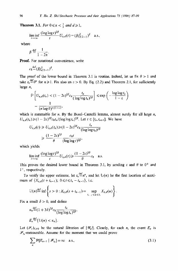
Theorem 1.1. For any d 2 1,

l im inf (1% 1% tj2 I’cc t

Ud(t) =j$2-1 a.%

where jdp-1 stands for the smallest positive root of Jd/2-1, the Bessel function of index (d/2 - 1).

Remark 1.2. Since j-r/z = 7t/2, taking d = 1 in Theorem 1.1, we immediately recover Theorem A.

(b) The above describes the location of maximum of /[fill in the time scale. If instead, we are interested in the location of maximum in the space scale, this will lead to the study of the favourite site of 1) I’& 11. The problem of favourite sites for one- dimensional Brownian motion is first attacked by Bass and Griffin (1985), who obtained some remarkable results. For more recent progress, cf. Eisenbaum (1989, 1990) and Leuridan (1997). We also mention relevant works of Eisenbaum (1997) for stable Levy processes, RCvCsz (1990, ch. 11) and Toth and Werner (1997) for random walks, and Khoshnevisan and Lewis (1995) for Poisson processes.

Our study here is particularly motivated by the recent work of Bertoin and Marsalle (1997), who establish the following integral test for the favourite site of drifted one- dimensional Brownian motion. Let WI be real-valued Brownian motion as before, and

fix a > 0. Let l(x) be the local time at infinity of WI(t)+&. Let c(r)%f inf{yaO: e(y) = supOQzCr e(z)}, which is the favourite site in [O,r] of the drifted Brownian motion.

Theorem B (Bertoin and Marsalle 1997). For any nondecreusing function f > 0,

lim inf f(r) ---l(r)={ La.,. *I”&{: }-. ~-+a3 r

It is known (cf. Yor, 1992) that the process WI(t) + at has exactly the same sample paths as a (transient) Bessel process, but with a different random clock. It seems natural to ask if their respective favourite sites have similar asymptotics.

Let d 33 which ensures the transience of wd, and define the local time at infin-

ity {L(r); 720) of ]]&I( as the density of occupation time: for any positive Bore1 function cp,

s am cP(II&(t)l])dt=

s O” cp(r)L(r)dr.

0

Define the fuvourite site in [0, r] of I] wd I( as

vd(r)dAf inf s > 0: L(s)= sup L(u) 1 O<u<r

The next is our main result for vd(r).

Y. Hu, Z. ShilStochastic Processes and their Applications 73 (1998) 87-99 89

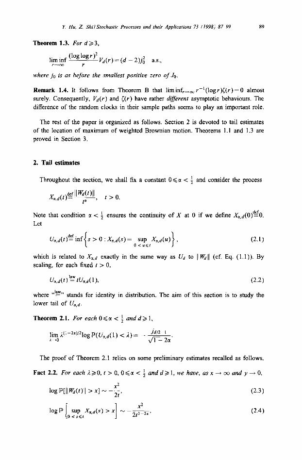
Theorem 1.3. For d >3,

l im inf (lot3 1% r12 Vd(v) = (d - 2)ji as., 1’00 r

where jo is as before the smallest positive zero of Jo.

Remark 1.4. It follows from Theorem B that liminf,,, r-‘(logr)[(r)=O almost surely. Consequently, V,(r) and c(r) have rather d$zrent asymptotic behaviours. The difference of the random clocks in their sample paths seems to play an important role.

The rest of the paper is organized as follows. Section 2 is devoted to tail estimates of the location of maximum of weighted Brownian motion. Theorems 1.1 and 1.3 are proved in Section 3.

2. Tail estimates

Throughout the section, we shall fix a constant O<cr < i and consider the process

Note that condition r < i ensures the continuity of X at 0 if we define &d(0)dZfO. Let

s > 0 : &d(s) = sup &J(u) , (2.1) o<ugr

which is related to &d exactly in the same way as ud to 11 wdll (cf. Eq. (1.1)). By scaling, for each fixed t > 0,

~a,d(t+=&,d(l), (2.2)

where “‘?’ stands for identity in distribution. The aim of this section is to study the lower tail of UU,d.

Theorem 2.1. For each 0 6 a -C i and d 2 1,

;$oJ (‘-2R)‘210g p(&d( 1) < ,i) = - $f&$.

The proof of Theorem 2.1 relies on some preliminary estimates recalled as follows.

Fact2.2. ForeachI2O,t>O,O~a<~andd21,wehave,asx~ooandy+O,

X2 log p[(I wd(t)ll ’ xl - -5’ (2.3)

log P sup &d(s) > X

I

X2 N --

ocs9r 2tl-Za’ (2.4)

90 Y Hu, Z. ShilStochastic Processes and their Applications 73 (1998) 87-99

l%P [ o Y!<, II Ws)lI < Y 1 i,2-lt

- -- . 2y2 ’

log P [

sup &d(S) < Y 1

j$2_lt’-2a - -

o<sgt 2(1 - 2a)y2’

[

II wd(s)ll 1ogP ___ oy$!&+A)CL <y 1 j&2_l((t + 1)lw2’ - L1-2a)

N - 2(1 - 2cr)y2 ’

(2.5)

(2.6)

(2.7)

where, the usual notation a(x) N b(x) (X + XO) means lim,,,, a(x)/@) = 1.

Remark 2.3. The estimate (2.3) is the well-known Mill’s ratio for Gaussian tails (cf. e.g. Shorack and Wellner, 1986, p. 850), whereas (2.4) is borrowed from a general theorem (for all bounded Gaussian processes) of Marcus and Shepp (1972). Note that the original statements of Eqs. (2.3) and (2.4) are for dimension one, but they can be easily extended to fit our setting. The lower tail (2.7) can be found in Berthet et al. (1997), which yields Eqs. (2.6) and (2.5) as special cases. We mention that Eq. (2.5) is in the classical work of Ciesielski and Taylor (1962), who actually identify the laws of (suP~<~~~ (1 &(,s)]])-’ and Brownian occupation time.

Proof of Theorem 2.1 (The upper bound). Write, for 0 < i < 1,

/iid~flFIU,,,(l) < n] = P [

II Wu)ll sup ~ AQUQI ua

< sup lIfwu)ll O<u<l 2.P 1 (2.8)

For any Y > 0, let lPr denote the probability under which I] Wd(] starts from r (therefore, PO = P). By the Markov property.

Al = WA& II Ki(J)Il, WI, (2.9)

where

odzf sup -, 11 @(“)ll O<u<l ua

and

(2.10)

with y denoting a vector in [Wd such that ]]y]] = y. Recall Anderson’s well-known inequality (cf. Anderson, 1955) for Gaussian shifted balls, which in our setting can be stated as

for any t > 0 and positive Bore1 function f. It follows that q(1; y, a) < q(12; 0, a). Going back to Eq. (2.9),

/iI < [E[q(& 0, @)I.

Y Hu, Z. Shil Stochastic Processes and their Applications 73 (1998) 87-99 91

Of course, we are only interested in the asymptotic behaviour of At when 1 tends to 0. Fix a small 6 > 0 and let J. E (0,6). According to Eq. (2.7), for any given E > 0,

there exists a constant c~~&~cI(E, 6, c(, d) > 0, depending only on (E, 6, a,d), such that for all x > 0,

P [ ,,::L

II wd(u)ll ___ <x (u + 6)” 1 ( -

<cl exp 41 6’-2”)

- 8) j&-,(1

2(, _ 2a)x2 ) Consequently, for all 2 E (0,6),

We can choose 6 dAf &E, LX) so small that (1 - E)( 1 - SlP2’) > 1 - 2~. By integration by parts, for A E (0,6),

where czdAfq(~, 6, IX, d) = (1 - 2.s)jii2_,cr/( 1 - 2~) is again a finite constant. According

to Eq. (2.4), there exists cgdAfq(~,~,d) > 0 depending only on (E,M,~), such that for all x > 0,

By scaling, 0 is distributed as 1tj2-a supo~,~ 1 &d(S). Consequently,

Al <c2c3 -( 1 - 2’:)2(Lj52;)X2 -(l-s)& . 1 J

Using Laplace’s method, it is easily checked that, for any

c5 > 0,

&log [lm $ exp (-3 - $)] N -2&Z,

given constants cd > 0 and

P --f 0,

which implies

lim sup A(1-2’)/210g Al < -

i-0 /yjd,i,.

Since E can be arbitrarily close to 0, this leads to the upper bound in Theorem 2.1.

92 Y. Hu, Z. Shil Stochastic Processes and their Applications 73 (1998) 87-99

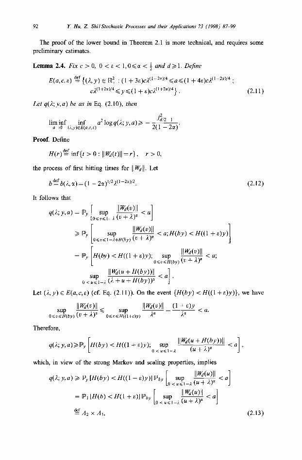
The proof of the lower bound in Theorem 2.1 is more technical, and requires some preliminary estimates.

Lemma2.4. Fixc>O, O<~<l,O~dl<~andd~l.De~ne

E(a, c, E) dAf {(A, y) E rw: : (1 + 3&)C1(‘-2m)‘4 <a 6 (1 + 4&)CA(‘-2x)‘4 ;

c/p+2a)/4 < y 6 (1 + +;l(‘+2a)/4} . (2.11)

Let q(J; y,a) be as in Eq. (2.10), then

lim inf inf a210gq(4y,a)> - &- 1

a-0 (Ay)EE(n,c,&) 2(1 - 2c()’

Proof. Define

H(r)kf inf{t > 0 : IIWd(t)ll =r}, Y > 0,

the process of first hitting times for 11 Wdll. Let

bEf b(& cI) = (1 _ 2,.41/2~(‘-2’“)i2. (2.12)

It follows that

3 yl < a; H(by) < H(( 1 + E)Y) 1 = py II wd(u)ll ~ <a; (u + A>

II wd(u + Wby))ll o <ttf-i. (A + u + H(by))” < ’ 1 ’

Let (A., y) E E(u, c, E) (cf. Eq. (2.11)). On the event {H(by) -c H(( 1 + a)~)}, we have

II wd(u)ll -d o<“s$(by) (0 + nY

sup IIwd(~)ll (1 + E)Y ___ = ___ <a. Oiu<H((l+s)y) 2” 1”

Therefore,

q(4 Y, a) 2 py Why) < H(( 1 + E)Y); sup II wd(u + Wv))ll O<u<l--l (24 + A)

which, in view of the strong Markov and scaling properties, implies

<a 3

1

1 d4 Y, a) a py W(by) < H((l + ~1~11 by II wd(u)ll

o<:$L(u+w <a J

= p, W(b) < ff( 1 + E)] pb, II wd(u)ll ~ <a 0 <?%.A (u + A) 1

d”f A2 x A3, (2.13)

Y. Hu, Z. ShilStochastic Processes and their Applications 73 (1998) 87-99 93

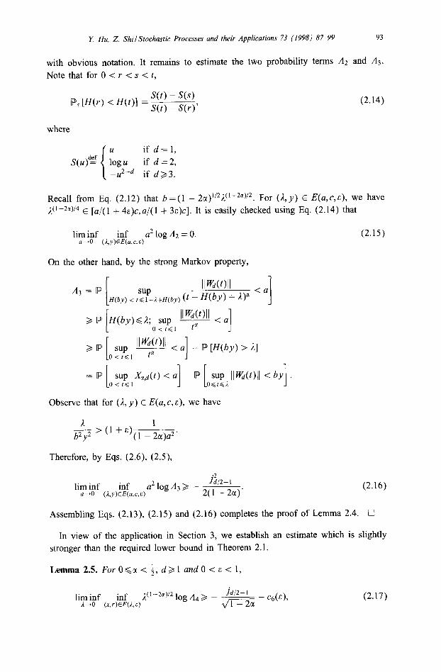
with obvious notation. It remains to estimate the two probability terms AZ and As. Note that for 0 < Y < s < f,

S(t) - S(s) ps W(r) < H(t)1 = s(t) _ S(r)’ (2.14)

where

Recall from Eq. (2.12) that b =(l - 2a) ‘1’ 2” (1-2r)/2. For (A, y) E E(a, c, E), we have

A(1-2’)/4 E [a/( 1 + 4s)c,a/(l + 3s)c]. It is easily checked using Eq. (2.14) that

lim inf inf Lz2 log n2 = 0. (2.15) a-0 (J0)Wa.G~)

On the other hand, by the strong Markov property,

A3 = P

[

II wd(t)ll

H(by) < r$f-A+H(by) (t - Wv) + 2)” < a 1 2 P [ H(by)<A; sup II wd(t)ll ~ <a

O<f<l tr 1 >P II @tt)ll sup ~ o<t<1 ta

<a -P[H(by)>i] I

= P SUP &J(t) < U - P SUP IIfi(t)ll -=C by . O<f$l 1 [ 0GfG-l I

Observe that for (A, y) E E(a, c, E), we have

k 1 - ’ (l +&)(I _ 2a)a2’ b2y2

Therefore, by Eqs. (2.6), (2.5),

lim inf inf a2log/13> - i/2- I

a+0 (kY)EE(%G&) 2(1 -2a)’ (2.16)

Assembling Eqs. (2.13) (2.15) and (2.16) completes the proof of Lemma 2.4. ??

In view of the application in Section 3, we establish an estimate which is slightly stronger than the required lower bound in Theorem 2.1.

Lemma2.5. ForOBa<~,dblandO<E,<l,

lim inf inf A-+0 (x,r)EF(i,&)

jL(1-2a)i2 log A4 > _ ~ _ (2.17)

94 Y Hu, 2. ShilStochastic Processes and their Applications 73 (1998) 87-99

where

and c~(E) > 0 is a jinite constant depending on (E, a,d) satisfying

hincs(&)=O

Proof. Assume (x, r) E F(1, E). From the Markov property it follows that

A4 = W(k II w,(~)Il,%

where

Let q(;1; y, a) be as before (cf. Eq. (2.10)). Obviously, g(1; y,a) >q(1; y,a) for all y 2 0 and a > 0. Therefore, for any fixed constant c > 0 (whose value is to be chosen later),

A4 3 L,[q(k II wd(n)ll, a3 L,[d4 II wn)ll, WE,13

where

_KldZf {&+*a)‘4 < (1 &(/?)I[ <( 1 + ,)Ca(1+2~)‘4;

[I&((1 - &)n)ll >(l + 3E)Ci(*+2N)‘4}.

On the event El, we have

~2 IIwd((’ - ‘)‘)I1 >(I + 3E)C$-2a)/4t$a(~) (r+(l -e)Ay’

Recall E(a,c,&) from Eq. (2.11). Since (A, II&(n)(l) E E(a(l),c,&), according to Lemma 2.4, for any fixed 6 > 0, when A is sufficiently small,

( ji,2- 1 A4 2 exp -(I + 6)2(1 _ 2aj(a(1jj2 P&W

= exp (1 + @ji,2-1

- 2( 1 Q,(G ). - 2a)( 1 + 3&)*c*N-*4*

It remains to bound below PJE1). Write

(2.18)

E2 kf {( 1 + 3~)cl-(‘-*4~ < II ~~(1 - s)ll

< ((1 + (3 + 3c-‘)E)C1-(‘-*~)~4}.

Y Hu, Z. ShilStochastic Processes and their Applications 73 11998) 87-99 95

By scaling,

P,(E, ) > Px[&(*--2@)‘4 < ]I w-( 1)]1 <( 1 + s)Ci-(1-*a)‘4,E2]

[ 1

(l+e)cI-“-z””

= be UEZ PC& IlKAl - &)ll,Z)~ > c;,-,‘-*x, 4 1

where p(t;x, y) denotes the semigroup of the d-dimensional Bessel process ]I II+]]. Recall (cf. Revuz and Yor, 1994, ch. XI) that

p(t;x,Jl) Iz 4 (;)d:2-’ exp (-‘7) Id/z_1 (y),

for all positive x and y. Here, &,2-l stands for the modified Bessel function. It is well known (cf. Lebedev, 1972) that Idj2_, (z) N 6/v’%& for z + co. Consequently, there

exists a finite constant c,~~~c~(E, c, GI, d) > 0, depending only on (E, c, a, d), such that for all small 1,,

i 1 (l+E)cr”-2z’~

Px(El) 3 c7b b, exp - Cl-,I-ZZ,.4 (

(IIwd(l -&Ill -4* & 2E

) 1 > c7cs~-U -2aP’ exp(-5( 1 + ,-‘)*E~~~--(‘-~~)‘~)[FD~(E~).

For (x, Y) E F(1, E),

(2.19)

P,(&) 3 P[]( Wd( 1 - &)I/ a( 1 + 3&)cJ-(1-21)‘4 + x] -PJ[]]wd(l - &)]I >(l + (3 + 3c-‘)E)c1~-(1-2”)~4 -x]

3 P[]]Wd(l - &)]I >(l + (3 + c-i)&)c1b-(‘--2Z)‘4]

-P[II&(l - E)l] >,(l + (3 + 2c-‘)&)c1-(1-2”)‘4],

which, in light of Eq. (2.3), yields

lim inf inf A(‘-2Z)‘2 log Px(E2) > - (1 + (3 + c-l)&)%?

J.--r0 (x,r)EF(l,c) 2(1-E) . (2.20)

Assembling Eqs. (2.18)-(2.20) yields that for all 0 < E < 1 and c > 0,

lim inf 1_o ,,,,;;&n,,:, $-2a)‘2 log A4

b- (1 + w$2_,

- 5( 1 + c-l )2&C2 - (1 + (3 + c-1)&)*c2

2( 1 - 2a)( 1 + 3&)&G 2(1 -&)

Taking cefji$t_ 1 /( 1 - 2~1)“~ and letting 6 tend to 0 yield Lemma 2.5. 0

Proof of Theorem 2.1 (the lower bound). Follows from Eq. (2.8) and Lemma 2.5. 0

3. Proofs of Theorems 1.1 and 1.3

We shall actually prove an extended version of Theorem 1.1. Let U%,d be as in Eq. (2.1).

96 Y. Hu, Z. ShilStochastic Processes and their Applications 73 (1998) 87-99

Theorem 3.1. For O<a < i andd31,

l irn inf m3 1% t)2p t-00 t &f(t) = (Pji,2_l 1” a.s.,

where

p!51. 1-2X

Proof. For notational convenience, write

csd~f(j3j;,2-,)P.

The proof of the lower bound in Theorem 3.1 is routine. Indeed, let us fix I3 > 1 and

take tndAfV’ for n > 1. Fix also an E > 0. By Eq. (2.2) and Theorem 2.1, for sufficiently large n,

p [

61 &d(b) < (l -2&)2P~8(loglogt,)2p ] <exp (-p)

1 = (n log o)lK--El ’

which is summable for n. By the Borel-Cantelli lemma, almost surely for all large n,

Uar,d(tn) > (1 - 2s)*Bcst,,/(log log tn)2p. Let t E [t,,, t,,+l]. We have

Uu,d(t) a G,d(Gl)>(l - w28c8 (log&p

~ (1 - 2&p C8t

0 (log log t)*fl ’ which yields

l im inf (1% log 02B u, d(t) > (1 - w28 , ’ 0 c8 a.s.

t-+m t

This proves the desired lower bound in Theorem 3.1, by sending E and 0 to O+ and l+, respectively.

To verify the upper estimate, let tndzfnn, and let U(n) be the first location of maxi-

mum of {&,d(t + b-1); Odtdt, - t,-I}, i.e.

Fix a small 6 > 0, and define

EnEf{ U(n) < K,}.

Let (9t)fa0 be the natural filtration of 11 Wdll. Clearly, for each n, the event E,, is Ftn-measurable. Assume for the moment that we could prove

C &%+I I Ftnl = 03 a.s., (3.1) n

Y. Hu, Z. ShilStochastic Processes and their Applications 73 (1998) 87-99 91

then by virtue of Levy’s Borel-Cantelli lemma (cf. Shiryaev, 1996, p. 518), we have P(&; i.o.) = 1, which in turn will imply

liminf (10g10gt’)28 U(n)<(l + 36)28~s as . . (3.2) Il-CXY tn

On the other hand, by the usual and weighted Chung laws of the iterated logarithm,

lim sup 1

t(‘-2@~z(loglogt)l~z c sup &J(S) = 2’12 a.s.,

t-03 <s<t

lim inf (1% 1% tv2 t*co &‘-2aV2 sup &d(s) = (2y4i;,,2 as.,

o<s<t

cf., respectively, R&&z ( 1990, Theorem 18.1) and Shi (1996). We point out that the usual law of the iterated logarithm is originally stated for &p(t) instead of

sup0 <s&&), b u a well-known o-by-o argument confirms that they have exactly t the same limsup behaviours, cf. C&go and R&&z (1981, p. 28).

Hence, almost surely for all large IZ, sup, r; sGt,_, X,,,(s) < sup0 < sGt,XX,d(~), which means U(n)= U&t,) - tn_l. In view of Eq. (3.2), we shall have proved

l im inf (log log tn >2” U&t,) < (1 + 36)2pcs a.s.

nP+cX tn

Since 6 > 0 can be chosen arbitrarily close to 0, this yields the desired upper estimate in Theorem 3.1.

It remains only to verify (3.1). Let O<w, 62(t,,loglog t,)“‘. We have

p[Gz+I I II Kdt,)ll = %I

=P [

sup II K@)ll > sup IIwd(s)ll 4 CS<Kn+l SZ &it1 aGt”+l s’ I Ilw,(tn)ll =wn 1

= pwn [

II wd(u)ll II wd(u)Il 0<2-t

sup ~ \.n+ ” (U ’ Kn+,-tn<uQt,+l-tn (u + tn)”

=P [

II Kdu)ll II wd(u)ll w.ldz og$A, (u + tnl4lY ’ ,“Z, (u + tn/&Y 1 ’

where A,dGft,,+l - t,, and &,def(~,,+i - t,,)/A,,. Let Q(E) be the constant introduced in (Eq. (2.17)). Since lim,+c G(E) = 0, it is possible to choose a (fixed) small E > 0 such that

$!z& + Cg(&) < (1 + S)S. vK?z

Observe that for all sufficiently large n,

98 Y. Hu, Z. ShilStochastic Processes and their Applications 73 (1998) 87-99

Since I, + 0 as n tends to infinity, applying Lemma 2.5 to xdzf ~,,/a, r dAf &/A,, and /z dAf A,, yields that, for all large II.

P[E,+l I II wd(t,)lI = wnl 2exp ( 41 + 26) A-(1-2a)/2 $1;

a n >

2 exp( -log log tn+l )

1

=(n+ l)log(n+ 1)

However, by the usual iterated logarithm law, almost surely for all large t, 11 Wd(t)ll < 2(t log log tp, which implies that, with probability one, for some (possibly random) finite no, if n ano, then

w%+1 I ~“l=wG+l I IIKi(t,)lll~(n+ l)lo;(n+ 1)’

which implies Eq. (3.1). Theorem 3.1 is proved. Cl

Proof of Theorem 1.1. Follows from Theorem 3.1 by taking 01 = 0. 0

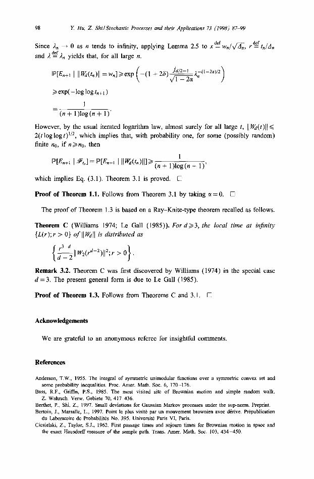
The proof of Theorem 1.3 is based on a Ray-Knite-type theorem recalled as follows.

Theorem C (Williams 1974; Le Gall (1985)). For d>3, the local time at injinity {L(r);r > 0) of I(WdII is distributed as

{ & 11 W2(rdp2)l12; r > 0) .

Remark 3.2. Theorem C was first discovered by Williams (1974) in the special case d = 3. The present general form is due to Le Gall (1985).

Proof of Theorem 1.3. Follows from Theorems C and 3.1. 0

Acknowledgements

We are grateful to an anonymous referee for insightful comments.

References

Anderson, T.W., 1955. The integral of symmetric unimodular functions over a symmetric convex set and some probability inequalities. Proc. Amer. Math. Sot. 6, 170-176.

Bass, R.F., Griffin, P.S., 1985. The most visited site of Brownian motion and simple random walk. 2. Wahrsch. Verw. Gebiete 70, 417436.

Berthet, P., Shi, Z., 1997. Small deviations for Gaussian Markov processes under the sup-norm. Preprint. Bertoin, J., Marsalle, L., 1997. Point le plus visit& par un mouvement brownien avec derive. Pmpublication

du Laboratoire de Probabilitb No. 395. Universite Paris VI, Paris. Ciesielski, Z., Taylor, S.J., 1962. First passage times and sojourn times for Brownian motion in space and

the exact Hausdortl measure of the sample path. Trans. Amer. Math. Sot. 103, 434-450.

Y Hu, Z. ShilStochastic Processes and their Applications 73 (1998) 87-99 99

Csaki, E., Foldes, A., R&&z, P., 1987a. On the maximum of a Wiener process and its location. Probab. Theory Related Fields 76, 477-497.

Csaki, E., Fiildes, A., Salminen, P., 1987b. On the joint distribution of the maximum and its location for a linear diffusion. Ann, Inst. H. Poincare Probab. Statist. 23, 179-194.

Csiirgo, M., Revtsz, P., 1981. Strong Approximations in Probability and Statistics. Academic Press, New York.

Eisenbaum, N., 1989. Temps locaux, excursions et lieu le plus visite par un mouvement brownien lineaire. These de Doctorat de I’Universite Paris VII, Paris.

Eisenbaum, N., 1990. Un theoreme de Ray-Knight lie au supremum des temps locaux browniens. Probab. Theory Related Fields 87, 27-34.

Eisenbaum, N., 1997. On the most visited sites by a symmetric stable process. Probab. Theory Related Fields 107, 527-535.

Imhof, J.P., 1984. Density factorization for Brownian motion, meander and the three-dimensional Bessel process, and applications. J. Appl. Probab. 21, 500-510.

Khoshnevisan, D., Lewis, T.M., 1995. The favorite point of a Poisson process. Stochastic Process. Appl. 57, 19-38.

Lebedev, N.N., 1972. Special Functions and their Applications. Dover, New York. Le Gall, J.-F., 1985. Sur la measure de HausdortI de la courbe brownienne. In: A&ma, J., Meyer, P.-A.,

Yor, M. (Eds.), Siminaire de Probabilitts XIX, Lecture Notes in Mathematics, vol. 1123. Springer, Berlin, pp. 297-313.

Leuridan, C., 1997. Le point d’un ferme le plus visit6 par le mouvement brownien. Ann. Probab. 25, 953-996. Marcus, M.B., Shepp, L.A., 1972. Sample behavior of Gaussian processes. In: Proc. 6th Berkeley Symp.

Mathematical Statistical Probability, vol. 2. University of California Press, Berkeley, pp. 4233441. Revtsz, P., 1990. Random Walk in Random and Non-Random Environments. World Scientific, Singapore. Revue, D., Yor, M., 1994. Continuous Martingales and Brownian Motion, 2nd ed., Springer, Berlin. Shi, Z., 1996. Small ball probabilities for a Wiener process under weighted sup-norms, with an application

to the supremum of Bessel local times. J. Theoret. Probab. 9, 915-929. Shiryaev, A.N., 1996. Probability, 2nd ed., Springer, New York. Shorack, G.R., Wellner, J.A., 1986. Empirical Processes with Applications to Statistics. Wiley, New York. Toth, B., Werner, W., 1997. Tied favourite edges for simple random walk. Preprint. Williams, D., 1974. Path decomposition and continuity of local time for one-dimensional diffusions. I, Proc.

London Math. Sot. 28, 738-768. Yor, M., 1992. Some Aspects of Brownian Motion. Part I: Some Special Functionals. Birkhauser, Basel.