a note of the completeness of preservation (isolated bone, group of bones, complete skull,complete skeleton) for each.
In the past, Western authors have tended to rename Russian svitas as ‘formations’, andgorizonts as ‘horizons’, but this masks their true meanings. In Russia, gorizonts are themain regional stratigraphic units, identified primarily from their palaeontologicalcharacteristics, and they do not pertain to lithostratigraphic units. Svitas are largelylithostratigraphic units, given a locality name that is close to their characteristic exposure.The definition of a svita incorporates a mix of field lithological observations andbiostratigraphic assumptions.
AnalysisThe records were converted into range charts (Fig. 1), including Lazarus taxa22, fromwhich total numbers (N) and numbers of originations (O) and extinctions (E) per timebin were calculated. Percentage origination and extinction metrics (O/N, E/N) werecalculated for each time bin (Fig. 2). There are many other possible measures of extinctionand origination rates, most calculated with respect to time; such measures would beinappropriate here because the durations of the svitas are poorly constrained. Boundary-crossing measures of extinction and origination rates were not used because the samplesizes are small, and 10 of the 38 families are restricted to one time bin and would have to bediscarded. Generic rates are not presented because many genera are singletons (restrictedto one time bin) and most are in need of taxonomic revision. Binomial error bars30 arecalculated for the percentage metrics.
The possible influence of sampling was assessed from the raw data (Fig. 3), and by theapplication of three sampling standardizations. In the first standardization, units that hadyielded fewer than 50 specimens were ignored (namely the Osinovskaya, Belebey,Bolshekinelskaya, Gostevskaya and Bukobay svitas); sample sizes then ranged from 49 to147 specimens. In the second sampling standardization, the two oldest units were ignored,and the others with small sample sizes were combined with adjacent units(Bolshekinelskaya þ Amanakskaya, Gostevskaya þ Petropavlovskaya,Donguz þ Bukobay), yielding a range of sample sizes from 50 to 147 specimens. In thethird sampling standardization, rarefaction analysis was applied to the units that hadyielded larger samples of specimens (Kopanskaya, Kzylsaiskaya, Staritskaya) to assesswhat their apparent diversity would have been had the sample size been 50, within therange 49–63 specimens, as for the other moderately well sampled units.
The data sets and analyses are available as Supplementary Data, and may bedownloaded at http://palaeo.gly.bris.ac.uk/Data/RussiaPTr.xls.
DatingThe timescale indicated in Fig. 1 is based on refs 10, 23, 24 and 25. The date for thePermian–Triassic boundary, 251 Myr, from ref. 10, has been debated26, but is widelyaccepted and will be the accepted date in the new Cambridge geologic timescale27,28. Otheraspects of the scales may seem less familiar, in that the Kazanian and Tatarian are muchlonger than is often assumed, 16 Myr instead of 4–5 Myr, and the Middle Triassic is datedas older than normally accepted. Should the old dates prove to be correct, and the newerones incorrect, the conclusions here are not affected because we do not make claims aboutthe longer-term timing of events, nor do we present rates of origination or extinctioncalculated against time.
Received 2 July; accepted 18 August 2004; doi:10.1038/nature02950.
1. Erwin, D. H. The Permo-Triassic extinction. Nature 367, 231–236 (1994).
2. Benton, M. J. When Life Nearly Died (Thames & Hudson, London, 2003).
3. Jin, Y. G. et al. Pattern of marine mass extinction near the Permian–Triassic boundary in south China.
Science 289, 432–436 (2000).
4. Sepkoski, J. J. Jr in Global Events and Event Stratigraphy (ed. Walliser, O. H.) 35–52 (Springer, Berlin,
1996).
5. Maxwell, W. D. Permian and Early Triassic extinction of nonmarine tetrapods. Palaeontology 35,
571–583 (1992).
6. Raup, D. M. Size of the Permo-Triassic bottleneck and its evolutionary implications. Science 206,
217–218 (1979).
7. McKinney, M. L. Extinction selectivity among lower taxa—gradational patterns and rarefaction error
in extinction estimates. Paleobiology 21, 300–313 (1995).
8. Twitchett, R. J., Looy, C. V., Morante, R., Visscher, H. & Wignall, P. B. Rapid and synchronous
collapse of marine and terrestrial ecosystems during the end-Permian biotic crisis. Geology 29,
351–354 (2001).
9. Benton, M. J. & Twitchett, R. J. How to kill (almost) all life: the end-Permian extinction event. Trends
Ecol. Evol. 18, 358–365 (2003).
10. Bowring, S. A. et al. U/Pb zircon geochronology of the end-Permian mass extinction. Science 280,
1039–1045 (1998).
11. Wignall, P. B. & Twitchett, R. J. Oceanic anoxia and the end Permian mass extinction. Science 272,
1155–1158 (1996).
12. Berner, R. A. Examination of hypotheses for the Permo-Triassic boundary extinction by carbon cycle
modeling. Proc. Natl Acad. Sci. USA 99, 4172–4177 (2002).
13. Newell, A. J., Tverdokhlebov, V. P. & Benton, M. J. Interplay of tectonics and climate on a transverse
Long-term decline in krill stockand increase in salps withinthe Southern OceanAngus Atkinson1, Volker Siegel2, Evgeny Pakhomov3,4 & Peter Rothery5
1British Antarctic Survey, Natural Environment Research Council, High Cross,Madingley Road, Cambridge CB3 OET, UK2Sea Fisheries Institute, Palmaille 9, 22767 Hamburg, Germany3Department of Earth and Ocean Sciences, University of British Columbia, 6339Stores Rd, Vancouver, British Columbia, V6T 1Z4, Canada4Department of Zoology, Faculty of Science and Technology, University of FortHare, Private Bag X1314, Alice 5700, South Africa5NERC Centre for Ecology and Hydrology, CEH Monks Wood, Abbots Ripton,Huntingdon PE28 2LS, UK.............................................................................................................................................................................
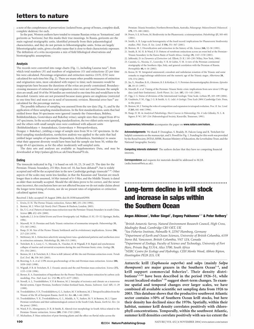
Antarctic krill (Euphausia superba) and salps (mainly Salpathompsoni) are major grazers in the Southern Ocean1–4, andkrill support commercial fisheries5. Their density distri-butions1,3,4,6 have been described in the period 1926–51, whilerecent localized studies7–10 suggest short-term changes. To exam-ine spatial and temporal changes over larger scales, we havecombined all available scientific net sampling data from 1926 to2003. This database shows that the productive southwest Atlanticsector contains >50% of Southern Ocean krill stocks, but heretheir density has declined since the 1970s. Spatially, within theirhabitat, summer krill density correlates positively with chloro-phyll concentrations. Temporally, within the southwest Atlantic,summer krill densities correlate positively with sea-ice extent the
previous winter. Summer food and the extent of winter sea iceare thus key factors in the high krill densities observed in thesouthwest Atlantic Ocean. Krill need the summer phytoplank-ton blooms of this sector, where winters of extensive sea icemean plentiful winter food from ice algae, promoting larvalrecruitment7–11 and replenishing the stock. Salps, by contrast,occupy the extensive lower-productivity regions of theSouthern Ocean and tolerate warmer water than krill2–4,12. Askrill densities decreased last century, salps appear to haveincreased in the southern part of their range. These changeshave had profound effects within the Southern Ocean foodweb10,13.
Our database comprises 11,978 net hauls from 9 countries,spanning the summers of 1926–39 and 1976–2003. This databaseshows a concentration of krill in the productive southwest (SW)Atlantic sector (Fig. 1a, b). On the basis of catches with equivalentnets (Supplementary Information), 58–71% of krill are locatedhere.
Potential krill habitat lies between the Polar Front (PF) to thenorth and the ice-covered Antarctic shelves to the south1,7,14, butkrill do not occupy all of this range. There are various explanationsfor regional variations in krill density, invoking the seasonal ice
Figure 1 Krill, salps and their food. a, Mean (November–April) chlorophyll a (chl a)
concentration, 1997–2003. b, Mean krill density (6,675 stations, 1926–2003). c, Mean
salp density (5,030 stations, 1926–2003). Log10(no. krill m22) ¼ 1.2 log10(mg chl a
m23) þ 0.83 (R 2 ¼ 0.051, P ¼ 0.017, n ¼ 110 grid cells). Historical mean positions
are shown for the PF29, Southern ACC Front (SACCF)30, SB30 and northern 15% sea-ice
concentrations in February and September (1979–2004 means).
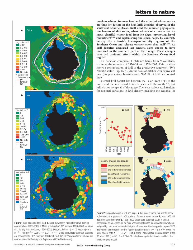
Figure 2 Temporal change of krill and salps. a, Krill density in the SW Atlantic sector
(4,948 stations in years with .50 stations). Temporal trends include b, post-1976 krill
data from scientific trawls; c, 1926–2003 circumpolar salp data south of the SB.
Regressions of log10(mean no. m22) on year were calculated for cells with$3 yr of data,
weighted by number of stations in that year. One-sample t-tests supported a post-1976
decrease in krill density in the SW Atlantic (scientific trawls: t ¼ 23.4, P ¼ 0.004, 16
cells, smaller nets: t ¼ 22.5, P ¼ 0.04, 8 cells). Salp densities increased south of the
SB after 1926 (t ¼ 3.1, P ¼ 0.004, 32 cells) Green spots denote cells usable in the
zone12,15 (SIZ), the Southern Boundary (SB) of the AntarcticCircumpolar Current16 (ACC) or the province to its south12. Butnone of these relationships hold at the circumpolar scale17. Forexample, krill densities are high near South Georgia, north of boththe SB and the SIZ (Fig. 1). However, all of these models link krilldensity to the abundance of food, which is likely to be the primaryfactor determining abundance. Together, sea ice, oceanography andnutrients promote primary production near shelves, fronts and iceedges18, and krill occupy this full range of habitats. Within thedistributional range of krill, their mean density correlates positivelywith the concentration of chlorophyll a (chl a; Fig. 1).
Salps tend to occupy warmer water than krill2–4,12, and preferoceanic regions with lower food concentrations2,3. Thus the lowerproductivity across most of the ACC means that the habitat of salpsis much larger than that of krill, with no concentration into onesector (Fig. 1c). The hotspot of krill in the SW Atlantic—a featurevery unlike that of zooplankton6—suggests an ability to maintaintheir 5–7-yr life cycle here, withstanding entrainment into the greatcurrent systems encircling Antarctica.
We studied temporal trends in krill and salp density using a grid,which incorporates inter-annual variability in density (Fig. 2a) intoa time-series regression within each of its cells. These are used inone-sample t-tests (for example, Fig. 2b, c) and a spatio-temporalmodel (Table 1). Salp densities increased south of the SB over thewhole time series. For krill in the SW Atlantic sector, densities havedeclined significantly since 1976.
Monitoring surveys7–10 show shorter-term changes in krill andsalp density. However, these are too localized to tell whether theyreflect changes in overall population size17. The trends reported hereare longer-term and over larger scales, supported by independentsurveys with scientific trawls (that is, Rectangular midwater
trawls and Isaac Kidd midwater trawls) and with smaller nets(Supplementary Information).
Controls on grazer populations include top-down (predation)and bottom-up (resource-based) factors17. We have examinedtemporal links between krill density and a key physical par-ameter—winter sea ice7–11. To find the appropriate scale for analysis,we compared krill densities between the eastern (308–508W) andwestern (508–708W) sub-areas of the SW Atlantic. Over the 19available summers, krill density in the east and west are positivelyrelated (R2 ¼ 0.47, P , 0.001). Whether this reflects advection19,20
or common controls on krill populations17, it suggests a basin-scalesynchrony in the inter-annual signal.
We therefore compared net data from the whole SW Atlantic toindices of sea ice. Here, summer krill density correlates to boththe duration (Fig. 3a) and the extent (Fig. 3b) of sea ice theprevious winter in the same area. Salps showed no such relation-ships, despite a negative one being postulated previously off theAntarctic Peninsula8. With shorter life cycles than krill and explosivepopulation growth rates, salps can respond to environmentalvariation over shorter timescales2–4.
The population size of krill has been linked both to predationcontols11,13,17,20,21 and to food resources within winter sea ice7–11. Ourresults are, to our knowledge, the first to show a direct, large-scalelink between annual krill density and sea-ice cover. This is not alocalized, short-term effect—it relates to .50% of their stock andthe data span 1926–2003. Given the problems of net sampling5, theexistence of a relationship with sea ice suggests that this factor playsa dominant role, not just in krill recruitment7–11, but also in theirpopulation size.
Various mechanisms have been proposed to explain how sea icebenefits krill7–11,22. Sea-ice algae are a critical food resource, boostingearly adult spawning in spring or survival of the larvae the followingwinter. Sea ice could also shield krill from predation. However, theonly link with summer krill density that we found was with ice coverthe preceding winter— ice cover from the winter before that had nosignificant effect. A 6-month lag points to larval over-wintering as akey process affected by ice—larvae need to survive their first winterto recruit the following summer, and thus replenish the adultpopulation. At the Antarctic Peninsula, only a few years of strongrecruitment per decade are needed to maintain the local krillpopulation7–11.
These positive temporal relationships between krill density andsea-ice extent (Fig. 3) do not equate to positive spatial relationships(Fig. 1a, b). High krill densities can be found at South Georgiaoutside the SIZ, whereas low densities coincide with an extensiveSIZ, for example, in the SW Indian sector. Hence sufficient winter icein the major spawning and nursery areas (the Antarctic Peninsulaand Southern Scotia Arc1,7,11,23) affects krill density across a wholeocean basin, including areas north of the SIZ. Krill larvae do notmerely need to survive the winter— they need to double in length11
Sufficient food year-round may thus be the feature of the SWAtlantic that maintains its high krill stocks.
The western Antarctic Peninsula is one of the world’s fastestwarming areas, and (atypically for the Southern Ocean) winter sea-ice duration in this sector is shortening24. Key spawning and nursery
Figure 3 Krill–ice relationships. Annual mean density of krill across the SW Atlantic versus
a, sea-ice duration27 (that is, days of fast ice observed at the South Orkneys the previous
winter), and b, the mean September latitude of 15% ice cover along a transect10 across
the western Scotia Sea. Regression identified one outlier season (1934, open circle) with
exceptionally long ice duration and only 24 net stations, so for the remaining years
log10(no. krill m22) ¼ 0.49 þ 0.0040 (sea-ice duration, days) R 2 ¼ 0.21, P ¼ 0.006,
n ¼ 35. Log10(no. krill m22) ¼ 14 þ 0.21 (sea ice latitude, degrees) R 2 ¼ 0.21,
P ¼ 0.02, n ¼ 25.
Table 1 Significant temporal trends krill and salp density
Taxon Subset of data analysed Estimated % increase (þ) ordecrease (2) per decade (s.e.m) P value
Era Net type Region...................................................................................................................................................................................................................................................................................................................................................................
Salps Post 1926 (34 yr) All Circumpolar (8 grid cells) þ66 (23) þ 87 (20) 0.007 , 0.001Krill Post 1976 (21 yr) Scientific trawls SW Atlantic (10 grid cells) 238 (24) 2 38 (15) 0.12 0.023Krill Post 1976 (14 yr) All other nets SW Atlantic (8 grid cells) 275 (21) 2 81 (16) 0.004 , 0.001...................................................................................................................................................................................................................................................................................................................................................................
A spatio-temporal model for log10 (no. krill or salps m22) with linear trend, grid cell effects, and including random year effects (upright font) or ignoring random year effects (italic font). See Methods.
areas of krill are thus located in a region that is sensitive toenvironmental change. Deep ocean temperatures have increased25,and a circumpolar, pre 1970s decrease in sea ice26 has been indicatedat several locations27,28. The regional decrease in a high-latitudespecies with high food requirements (krill) coincides with anincrease in a lower-latitude group with lower food requirements(salps). However, as the mechanisms underlying these changes areuncertain, future predictions must be cautious.
These changes among key species have profound implications forthe Southern Ocean food web. Penguins, albatrosses, seals andwhales have wide foraging ranges but are prone to krill short-age5,10,13,21. Thus the wide extent of our indicated change in krilldensity— not just its magnitude— is important. The basin-scaledecline in krill may underlie the post 1980s shift in demographyof krill predators, seen across the SW Atlantic10,13. Earlier lastcentury, over-exploitation of whales preceded a rapid increase insmaller krill predators such as fur seals in the SWAtlantic20,21. Addedto this shift in the predator balance, a return of the whales to pre-exploitation levels now faces the further problem of lower krilldensity. A
MethodsSatellite dataAverage values of SeaWiFS Level-3 standard mapped images of chl a concentration werecalculated in Arc GIS 8.2 for grid cells with data for November–April (Fig. 1a). Sea-iceimages, calculated from DMSP-SSMI passive microwave data by NOAA/NCEP, were pre-viewed as the northern extent of 15% ice concentration to remove spurious values beforecalculating mean monthly positions.
The krill and salp databaseThe full database (Supplementary Table 2) comprises data from the UK, Germany, USA,the Ukraine, South Africa, Japan, Australia, Poland and Spain. All are non-targetedoblique or vertical hauls from pre-fixed positions. The data were either from samplessorted by the authors, available within our institutes, sent by our collaborators, ortranscribed from the literature. Krill densities (no. m22) include only postlarvae, or justthe krill .19 mm long from the Discovery (1926–51) era. Salp densities are the totalsolitary plus aggregate individuals of S. thompsoni and the rarer Ihlea racovitzai, pooled toavoid identification problems. Historical Discovery data (1926–51) were cross-checkedfrom three archived sources: the net sampling logs, the original tables used to construct thepublished figures1,4, and an electronic krill database. The Discovery Report Station Lists1,4
were used to calculate densities.
Extraction and analysis of dataFrom the full database, we extracted November–April data south of the PF where at leastthe topmost 75 m (krill) or 100 m (salps) was sampled. Sampling was mainly much deeper(Supplementary Table 3) and 90% was in December–March. Regression of krill density onchl a concentration (Fig. 1) used mean grid cell values, and was restricted to post-1976scientific trawl data in cells where krill were caught.
We tested spatio-temporal trends among: stations south of the PF, PF to SB, south ofthe SB, the post 1926 era, the post 1976 era, the SW Atlantic sector only and circumpolar.We report only trends significant in two tests—first, a one-sample t-test of whether theregression slopes of cells (Fig. 2) differ from zero, supporting a widespread shift inabundance. Second, to further test for a temporal trend we used a spatio-temporal model:y kt ¼ g k þ bt þ B t þ E kt, where y kt is the log10 transformed mean density (þc) in gridsquare k and season t, g k is a fixed effect for grid square k, b is the slope, the average changeper season on a log10 scale, Bt is a random effect for season t and E kt is a random square byseason effect. The constant c (added to allow for log transformation of zero densities) washalf the minimum density. The variance of the cell-season effect was assumed to beinversely proportional to the number of net hauls (nkt) for each cell-season combination.Cells with sufficient data for inclusion in the mixed model (Fig. 2) were defined as thosewith at least 5 seasons and 50 stations. The model was fitted by residual maximumlikelihood, with the t-test for trend based on n 2 2 degrees of freedom, where n is thenumber of seasons. A general linear model ignoring the random year effect (that is, thevalues shown in italics in Table 1), gave similar estimated slopes but smaller standarderrors—an effect of pseudo-replication from treating the observations as statisticallyindependent.
Potential sampling artefactsThe asymmetrical circumpolar distribution of krill density persisted last century and issupported independently by differing sampling gear (Supplementary Fig. 4) Our spatio-temporal analyses encompass broad-scale spatial differences in sampling location, butSupplementary Fig. 5 shows that at finer scales, sampling has focused increasingly ontoproductive shelf/shelf break areas favoured by krill14,17 but not by salps2,3. The trends arethus not artefacts of sampling emphasis. Likewise, any systematic changes in samplingmethod (Supplementary Table 3) observed would tend to increase krill density in recentyears rather than decrease it. Station positions were pre-fixed, so generally sampled onarrival—that is, at random times of the day or night, thus not biasing our grid-based
analyses. The sea-ice relationships were supported by multiple subsets of krill data and
sea-ice indices (Supplementary Table 4).
Received 17 May; accepted 7 September 2004; doi:10.1038/nature02996.
1. Marr, J. W. S. The natural history and geography of the Antarctic krill (Euphausia superba Dana).
Discovery Rep. 32, 33–464 (1962).
2. Le Fevre, J., Legendre, L. & Rivkin, R. B. Fluxes of biogenic carbon in the Southern Ocean: roles of large
microphagous zooplankton. J. Mar. Syst. 17, 325–345 (1998).
3. Pakhomov, E. A., Froneman, P. W. & Perissinotto, R. Salp/krill interactions in the Southern
Ocean: spatial segregation and implications for the carbon flux. Deep-Sea Res. II 49, 1881–1907
(2002).
4. Foxton, P. The distribution and life history of Salpa thompsoni Foxton with observations on a related