Abstract—A time domain frequency dependent model for transmission lines in low frequency range is proposed. The model considers the frequency dependent parameters of overhead conductors and soils. The targeted frequency range is zero to 1.2 kHz which is sufficient for geomagnetically induced current analysis in transmission circuits. The accuracy of the model in this frequency range is documented by comparing it to Carson’s equations. The proposed model achieves high accuracy with minimal computational burden. The use of the model is illustrated with a GIC test case analysis.
Index Terms— frequency dependent, geomagnetically induced current, transmission line model, time domain simulation
I. INTRODUCTION
Geomagnetically induced current (GIC) is the quasi direct current flowing in transmission lines and transformers as a results of a geomagnetic disturbance (GMD) [1]. One of the major effect of GIC is the half-cycle saturation in transformers, resulting in harmonics 2nd order to 20th order from distorted magnetizing current [2]–[4]. Considering the quasi dc GIC and harmonics, the frequency dependence of transmission line parameters, grounding system parameters, etc. should not be neglected. Due to skin effect, the equivalent impedance of a conductor is not constant as frequency varies. One way to consider the frequency dependence of transmission line parameters is to perform the analysis in frequency domain and transform the responses back to time domain using inverse Fourier transformation [5], [6]. This approach is accurate in theory, and has been integrated in some power system transient solvers. However, this approach is laced with a heavy computational burden because they require the computation of convolution integrals in each time step. Reference [7] discussed the integration of frequency dependent grounding impedances into a frequency dependent power line model; inverse Fourier transforms were used for impulse response in time domain.
Another approach is to mimic this frequency property in time domain using lumped circuit elements. Many of existing models use R-L ladder, Cauer or Foster network [8], or a fictional (equivalent) impedance network, to represent the frequency dependent conductor. One reasonable way to determine the element in this network is to divide the conductors into many parts, such as filaments or layers, and the elements are associated with resistance and inductance of these physical parts. Based on an approximate solution of Maxwell equations for a round conductor, Yen et al. [9] proposed a method to divide conductors into rings. The thickness of the rings is chosen to achieve a constant resistance ratio between
rings. Kim et al. in [10] modified Yen’s method by introducing ratio between inductance of layers. However, in order to make sure the equivalent inductance approximates well the exact value, the solution of a high order polynomial equation is needed. A four-layer case involves a fourth order polynomial, and this approach becomes restricted as the number of layers grows. Sen et al. [11] works on an even larger frequency range (up to few GHz). They directly provide a list of recommended resistance and inductance for the inner most branch, and the other branches are formulated by multiplying by an empirical value. The computational burden is largely reduced, but the resulting network has low accuracy and lacks physical meaning. For improved accuracy, Acero, et al. [12] calculated the magnetic energy in each layer and introduce the mutual inductance between layers to the network. Similarly, models in [13] also considered mutual inductance between layers of conductors. Reference [14] introduced the dual Cauer circuit by relating electric circuits to magnetic circuits, using magnetic flux and reluctance to represent the inductance of layers. Another approach does not depend on physical explanation [15]–[19] but they optimize the circuit to reproduce the line frequency characteristics using fitting methods. There are also attempts to model skin effect of rectangular conductors. In [20], [21], the authors divided the section into a large number of small rectangular sections, and [21] also proposed a method to reduce the dimension of equivalent network to achieve a balance between accuracy and computational burden. With the exception of reference [7], the literature practically ignores the frequency dependence of the soil parameters.
This paper proposes a low broadband transmission line model based on physical properties of transmission lines with clear physical explanation (physically based model). The model captures the frequency dependence of line conductors and the soil. The proposed method is easy to implement and yields accurate results in the frequency range of interest for the GIC analysis.
II. MOTIVATION
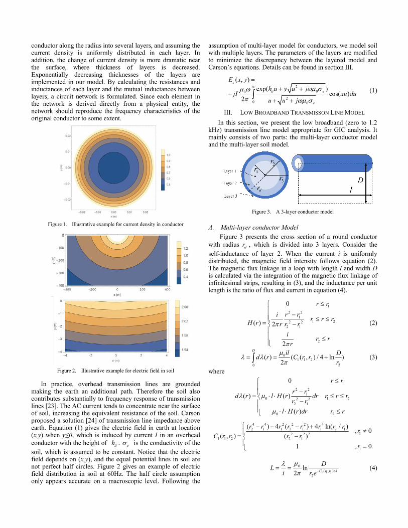
Skin effect leads to higher current densities near the surface of a conductor. By solving Maxwell equations for a cylindrical conductor, the exact current distribution over the cross section of a round conductor can be obtained. The current density at radius r is given in terms of modified Bessel functions [22]. Figure 1 depicts the normalized magnitude of current density in a large round conductor at 60Hz.
In order to mimic the uneven distribution of current, we propose a multi-layer conductor model by dividing the
conductor along the radius into several layers, and assuming the current density is uniformly distributed in each layer. In addition, the change of current density is more dramatic near the surface, where thickness of layers is decreased. Exponentially decreasing thicknesses of the layers are implemented in our model. By calculating the resistances and inductances of each layer and the mutual inductances between layers, a circuit network is formulated. Since each element in the network is derived directly from a physical entity, the network should reproduce the frequency characteristics of the original conductor to some extent.
Figure 1. Illustrative example for current density in conductor
Figure 2. Illustrative example for electric field in soil
In practice, overhead transmission lines are grounded making the earth an additional path. Therefore the soil also contributes substantially to frequency response of transmission lines [23]. The AC current tends to concentrate near the surface of soil, increasing the equivalent resistance of the soil. Carson proposed a solution [24] of transmission line impedance above earth. Equation (1) gives the electric field in earth at location (x,y) when y≤0, which is induced by current I in an overhead conductor with the height of iih . e is the conductivity of the soil, which is assumed to be constant. Notice that the electric field depends on (x,y), and the equal potential lines in soil are not perfect half circles. Figure 2 gives an example of electric field distribution in soil at 60Hz. The half circle assumption only appears accurate on a macroscopic level. Following the
assumption of multi-layer model for conductors, we model soil with multiple layers. The parameters of the layers are modified to minimize the discrepancy between the layered model and Carson’s equations. Details can be found in section III.
0
20
20
0
( , )exp( )
cos( )2
z
ii e
e
E x yh u y u j
jI xu duu u j
(1)
III. LOW BROADBAND TRANSMISSON LINE MODEL
In this section, we present the low broadband (zero to 1.2 kHz) transmission line model appropriate for GIC analysis. It mainly consists of two parts: the multi-layer conductor model and the multi-layer soil model.
Figure 3. A 3-layer conductor model
A. Multi-layer conductor Model
Figure 3 presents the cross section of a round conductor with radius dr , which is divided into 3 layers. Consider the self-inductance of layer 2. When the current i is uniformly distributed, the magnetic field intensity follows equation (2). The magnetic flux linkage in a loop with length l and width D is calculated via the integration of the magnetic flux linkage of infinitesimal strips, resulting in (3), and the inductance per unit length is the ratio of flux and current in equation (4).
1
2 21
1 22 22 1
2
0
( ) 2
2
r
r rir r
H r
r
rr
r
r
i
r
r
r
(2)
01 1 2
20
( ( , ) / 4 l( )2
) nD il D
Cd rr
r r
(3)
where
1
2 21
0 1 22 22 1
0 2
0
( )( )
( )
r
r
r
r rl H r dr r rd
r
rr r
l H r dr r
4 4 2 2 2 42 1 1 2 1 1 2 1
12 2 21 1 2 2 1
1
( ) 4 ( ) 4 ln( /0
0
),
( , ) ( )
1 ,
r r r r r r r rr
C r r r r
r
1 1 2
0
2( , ) / 4
ln2 C r r
D
riL
e
(4)
Next, we can calculate the mutual inductance between layers. The mutual inductance between layer 2 and layer 3 is given in equation (5). Similar procedure applies to other layers.
023 32 2 2 3
3
( ( , ) ln )2
DL L C r r
r
(5)
where
2 2 23 2 2 3 2
2 2 3 2 23 2
( ) / 2 ln /( , )
r r r r rC r r
r r
In addition, the mutual inductance is determined by the outer layer, i.e. 13 31 23 32L L L L . Assuming the overhead transmission line is placed over soil with perfect conductivity ( e ), then 2 iD h , ih is the height of conductor. In general, a n-layer impedance network for a conductor is represented by the following equation (6), in which 1m n .
1
( )( ) ( ) ( )kk
d tt v t
tv t
d i
R i L (6)
where
11 21 321
21 22 322
32 32 333
...
..., ...
... ... ... ......
nm
nm
nm
nm
n nm nm nm nm nm
L L L LRL L L LRL L L LR
LR L L L L L
R L
The resistance matrix R is composed of the resistance of each layer. i(t) is the vector of currents through each layer. The capacitance and conductance of the transmission line introduce shunt elements connected only to the outer layer of a conductor. To summarize, we represent a small length of a single-conductor transmission line with a π model as shown in figure 4. This model is a time domain model which can also be converted to a frequency domain equivalent )(eqZ that is
frequency dependent. Using similar approach, we can construct the model of an n-conductor transmission line.
Figure 4. Pi model for multilayer-conductor example
B. Multi-layer soil Model
Next, we include the influence of soil with finite conductivity. In order to explain our approach, we first consider the soil as forming an imaginary “soil ring” around the overhead conductor. Rudenberg [25] considered this approach and then used conformal mapping to derive the impact of semi-infinite soil model on the line parameters. Figure 5 shows an
example of a single conductor in the soil ring. eD is the equivalent thickness of the soil. When the frequency of current in the overhead conductor is very low, the magnetic field in the soil spreads over an extremely large area. For practical reasons, we can choose eD based on the frequency range we are interested in. In this approximate soil ring, the same calculation procedure for inductance of conductor layers is applicable. This approximation is less reliable near the surface of soil. We propose additional modifications to better represent the effect of the soil. Specifically, we replace R in equation (6) with αR .
Figure 5. Multi-layer soil model
The scaling matrix α can transform the resistance of the soil rings to better fit the real characteristics of the soil. The following empirical formula (7) used in this paper yields satisfactory results. To further improve the fitting, an optimization procedure may help determine α.
2.5( 1) / ( 1) 1; 0,ii ijn i n i j (7)
After calculating the self inductance of each soil layer, the mutual inductance between soil layers, and the mutual inductance M between soil and conductor layers, the low broadband transmission line model is constructed. Figure 6 shows the transmission line model with multi-layer conductor and multi-layer soil.
Figure 6. Pi model for broadband transmission line model example
IV. VALIDATION TESTS
A. Multi-layer conductor model
The accuracy of the proposed multi-layer conductor model is validated by comparing its equivalent impedance with the
well-known analytical solution in the frequency domain [22]. The theoretical solutions calculated from Bessel functions are denoted as “ref”; the proposed model is denoted with “3 layer”, “5 layers” and “10 layers” indicating the number of layers. In addition, a constant impedance model is derived from the exact impedance at 60Hz. Figures 7 and 8 show that the proposed model reproduces the frequency characteristics of the conductor accurately. A 5-layer model performs well with 1% error in resistance and 0.1% error in inductance.
In addition, this model performs well in high frequency by increasing the number of layers. Though not shown in figures, A 10-layer model remains accurate as the frequency increases to a few MHz.
Figure 7. Multi-layer conductor model resistance comparison
Figure 8. Multi-layer conductor model inductance comparison
B. Multi-layer soil model
The multi-layer soil model is compared with solutions from Carson’s equations. In Figures 9 and 10, we can observe that the proposed method shows larger deviation from reference value as the frequency grows. However, the overall accuracy is still satisfactory considering the simplicity of the proposed model. A 7-layer model yields 5% error in resistance and 1 %
error in inductance. On the other hand, the constant impedance model shows very large errors which lead to inaccurate analysis of GIC.
Figure 9. Multi-layer soil model resistance comparison
Figure 10. Multi-layer soil model inductance comparison
Figure 11. Testing system for GIC analysis
C. GIC analysis
The low broadband transmission line model is integrated into a power system model to study the effects of GIC on the power system and to examine its performance. Figure 11 shows the network configuration for the GIC analysis. The system includes a 24-km line which is modeled as a low broadband transmission line model. For comparison, we use the same system where the line is modeled using the 60Hz parameters of the line. The GMD induced a 5V/km field, which starts at time 0.75s. Figure 12 presents the DC current flowing through
transformer 2. The figure shows that the proposed model results in higher GIC than constant impedance line model. In other words, the 60 Hz model of the line tends to underestimate the GIC by a substantial percentage. Harmonics of transmission line phase voltages are analyzed in Figure 13. We can observe that the broadband model also yields higher harmonics on the transmission line.
Figure 12. Multi-layer soil model inductance comparison
Figure 13. Harmonics in tranmission line phase voltage – normalized to
fundamental
V. CONCLUSIONS
This paper presents the derivation of a time-domain frequency dependent transmission line model for a low frequency band. The model captures the frequency dependence characteristics of the power conductors and the soil. The accuracy of this low broadband model is validated. Simulation results show that for GIC analysis the model provides an accurate method for computing DC as well as harmonics generated by GIC. The model is presently used for comprehensive GIC impact studies.
ACKNOWLEDGMENT
The authors gratefully acknowledge the support of PG&E of this work.
REFERENCES [1] J. G. Kappenman, “Effects of Geomagnetic Disturbances on Power
Systems,” IEEE Power Eng. Rev., vol. 9, no. 10, pp. 15–20, 1989. [2] X. Dong, Y. Liu, and J. G. Kappenman, “Comparative analysis of exciting
current harmonics and reactive power consumption from GIC saturated transformers,” in Power Engineering Society Winter Meeting, IEEE, 2001, vol. 1, pp. 318–322.
[3] M. Lahtinen and J. Elovaara, “GIC occurrences and GIC test for 400 kV system transformer,” IEEE Trans. Power Deliv., vol. 17, no. 2, pp. 555–561, 2002.
[4] S. Lu, Y. Liu, and J. De La Ree, “Harmonics generated from a DC biased transformer,” IEEE Trans. Power Deliv., vol. 8, no. 2, pp. 725–731, 1993.
[5] A. Morched, B. Gustavsen, and M. Tartibi, “A universal model for accurate calculation of electromagnetic transients on overhead lines and underground cables,” IEEE Trans. Power Deliv., vol. 14, no. 3, pp. 1032–1038, 1999.
[6] A. Budner, “Introduction of frequency-dependent line parameters into an electromagnetic transients program,” IEEE Trans. Power Appar. Syst., no. 1, pp. 88–97, 1970.
[7] G. J. Cokkinides and A. P. Meliopoulos, “Transmission line modeling with explicit grounding representation,” Electr. Power Syst. Res., vol. 14, no. 2, pp. 109–119, 1988.
[8] S. Jazebi, F. de Leon, and B. Vahidi, “Duality-Synthesized Circuit for Eddy Current Effects in Transformer Windings,” IEEE Trans. Power Deliv., vol. 28, no. 2, pp. 1063–1072, Apr. 2013.
[9] C.-S. Yen, Z. Fazarinc, and R. L. Wheeler, “Time-domain skin-effect model for transient analysis of lossy transmission lines,” Proc. IEEE, vol. 70, no. 7, pp. 750–757, 1982.
[10] S. Kim and D. P. Neikirk, “Compact equivalent circuit model for the skin effect,” in Microwave Symposium Digest, 1996., IEEE MTT-S International, 1996, vol. 3, pp. 1815–1818.
[11] B. K. Sen and R. L. Wheeler, “Skin effects models for transmission line structures using generic SPICE circuit simulators,” in Electrical Performance of Electronic Packaging, IEEE 7th Topical Meeting on, 1998, pp. 128–131.
[12] J. Acero and C. R. Sullivan, “A dynamic equivalent network model of the skin effect,” in Applied Power Electronics Conference and Exposition (APEC), Twenty-Eighth Annual IEEE, 2013, pp. 2392–2397.
[13] A. E. Davies, Y. K. Tong, P. L. Lewin, and D. M. German, “A frequency-independent circuit model of a conductor under surge conditions,” Int. J. Numer. Model. Electron. Netw. Devices Fields, vol. 8, no. 2, pp. 139–147, 1995.
[14] P. Holmberg, M. Leijon, and T. Wass, “A wideband lumped circuit model of eddy current losses in a coil with a coaxial insulation system and a stranded conductor,” IEEE Trans. Power Deliv., vol. 18, no. 1, pp. 50–60, Jan. 2003.
[15] J. H. Krah, “Optimum discretization of a physical Cauer circuit,” IEEE Trans. Magn., vol. 41, no. 5, pp. 1444–1447, May 2005.
[16] C. Stackler, F. Morel, P. Ladoux, and P. Dworakowski, “25 kV–50 Hz railway supply modelling for medium frequencies (0–5 kHz),” in Electrical Systems for Aircraft, Railway, Ship Propulsion and Road Vehicles & International Transportation Electrification Conference (ESARS-ITEC), International Conference on, 2016, pp. 1–6.
[17] M. Sarto, A. Scarlatti, and C. Holloway, “On the use of fitting models for the time-domain analysis of problems with frequency-dependent parameters,” in Electromagnetic Compatibility, EMC. IEEE International Symposium on, 2001, vol. 1, pp. 588–593.
[18] S. Asgari, J. O. Oti, and J. N. Subrahmanyam, “Lossy skin effect modeling of interconnects,” in Magnetics Conference, INTERMAG Digest of Technical Papers. IEEE International, 2000, pp. 426–426.
[19] A. Semlyen and A. Deri, “Time domain modeling of frequency dependent three-phase transmission line impedance,” IEEE Power Eng. Rev., no. 6, pp. 64–65, 1985.
[20] W. T. Weeks, L.-H. Wu, M. F. McAllister, and A. Singh, “Resistive and inductive skin effect in rectangular conductors,” IBM J. Res. Dev., vol. 23, no. 6, pp. 652–660, 1979.
[21] S. Mei and Y. I. Ismail, “Modeling skin and proximity effects with reduced realizable RL circuits,” IEEE Trans. Very Large Scale Integr. VLSI Syst., vol. 12, no. 4, pp. 437–447, Apr. 2004.
[22] A. P. Meliopoulos, Power system grounding and transients: an introduction, Marcel Dekker, Inc., 1988.
[23] A. D. Papalexopoulos and A. P. Meliopoulos, “Frequency dependent characteristics of grounding systems,” IEEE Trans. Power Deliv., vol. 2, no. 4, pp. 1073–1081, 1987.
[24] J. R. Carson, “Wave propagation in overhead wires with ground return,” Bell Syst. Tech. J., vol. 5, no. 4, pp. 539–554, 1926.
[25] R. Rudenberg, “Grounding principles and practice I—Fundamental considerations on ground currents,” Electr. Eng., vol. 64, no. 1, pp. 1–13, 1945.