Biased Tracers in Redshift Space

in the EFT of Large-Scale Structure

Ashley Perko1,2, Leonardo Senatore1,2,3,

Elise Jennings4,5, and Risa H. Wechsler2,3

1 Stanford Institute for Theoretical Physics,

Stanford University, Stanford, CA 94306

2 Department of Physics,

Stanford University, Stanford, CA 94305

3 Kavli Institute for Particle Astrophysics and Cosmology and Dept. of Particle Physics and

Astrophysics, SLAC, Menlo Park, CA 94025

4 Center for Particle Astrophysics, Fermi National Accelerator Laboratory MS209,

P.O. Box 500, Kirk Rd. & Pine St., Batavia, IL 60510-0500

5 Kavli Institute for Cosmological Physics,

Enrico Fermi Institute, University of Chicago, Chicago, IL 60637

Abstract

The Effective Field Theory of Large-Scale Structure (EFTofLSS) provides a novel formalism that is

able to accurately predict the clustering of large-scale structure (LSS) in the mildly non-linear regime.

Here we provide the first computation of the power spectrum of biased tracers in redshift space at

one loop order, and we make the associated code publicly available. We compare the multipoles

` = 0, 2 of the redshift-space halo power spectrum, together with the real-space matter and halo

power spectra, with data from numerical simulations at z = 0.67. For the samples we compare

to, which have a number density of n = 3.8 · 10−2(hMpc−1 )3 and n = 3.9 · 10−4(hMpc−1 )3,

we find that the calculation at one-loop order matches numerical measurements to within a few

percent up to k ' 0.43hMpc−1 , a significant improvement with respect to former techniques.

By performing the so-called IR-resummation, we find that the Baryon Acoustic Oscillation peak

is accurately reproduced. Based on the results presented here, long-wavelength statistics that are

routinely observed in LSS surveys can be finally computed in the EFTofLSS. This formalism thus is

ready to start to be compared directly to observational data.

arX

iv:1

610.

0932

1v1

[ast

ro-p

h.C

O]

28 O

ct 2

016

FERMILAB-PUB-16-420-A

This manuscript has been authored by Fermi Research Alliance, LLC under Contract No. DE-AC02-07CH11359 with the U.S. Department of Energy, Office of Science, Office of High Energy Physics

Contents

1 Introduction 2

2 Biased tracers in real space 4

2.1 Review of δh perturbative expansion . . . . . . . . . . . . . . . . . . . . . . . . . . . 4

2.2 The velocity divergence as a biased density tracer . . . . . . . . . . . . . . . . . . . . 7

2.3 Stochastic halo bias . . . . . . . . . . . . . . . . . . . . . . . . . . . . . . . . . . . . 8

3 Biased tracers in redshift space 9

3.1 Review of the EFT of halos in redshift space . . . . . . . . . . . . . . . . . . . . . . 9

3.2 Stochastic halo bias in redshift space . . . . . . . . . . . . . . . . . . . . . . . . . . . 12

3.3 Halo-halo power spectrum in redshift space . . . . . . . . . . . . . . . . . . . . . . . 13

4 IR resummation 15

5 Fits to simulations 17

5.1 Fits to Galaxies . . . . . . . . . . . . . . . . . . . . . . . . . . . . . . . . . . . . . . . 21

6 Conclusion 22

A Halo kernels 23

B Degeneracy of halo bias parameters 25

C Redshift-space kernels 27

D The IR-safe integrand 28

E More details of the IR-resummation 30

F A Further Check of the Fitting Procedure 32

G Details of Parameter Fits 33

1 Introduction

In the next decade, large-scale structure data, collected through galaxy surveys, the CMB and

possibly 21cm emission, will be essential for our progress in understanding the first instants of the

universe and the late time growth of structures. In order to fully profit from this collection of data,

it will be important to be able to make theoretical predictions with comparable or better accuracy

than the errors in the observations. Current techniques have not yet achieved this goal in many

regimes. Numerical simulations have been the leading tool for predicting the clustering of large-

scale structure so far. However, keeping pace with the data to achieve the required accuracy over

the full range of parameter space needed will be challenging [1]. On the analytic side, in recent

2

years the Effective Field Theory of Large-Scale Structure 1 (EFTofLSS) [2, 3, 4, 5] has provided a

tool where predictions in the mildly non-linear regime can be delivered with an at-least-in-principle

arbitrary theoretical precision, and most probably with a precision that should be enough for next

generation experiments [2, 3, 4, 5, 6, 7, 8, 9, 10, 11, 12, 13, 14, 15, 16, 17, 18, 19, 20, 21, 22, 23, 24,

25, 26, 27, 28, 29, 30, 31].

This paper represents the culmination of a journey: we bring the theoretical construction of the

EFTofLSS all the way to computing statistics of the galaxy distribution in redshift space, which

can be compared directly with observational data from large-scale structure surveys. Computing

such observables is indeed a complex endeavor. In order to predict a given correlation function of

galaxies, one needs first to predict correlation functions of dark matter, then of biased tracers, and

then one has to map these correlation functions into redshift space. Each of these steps requires

novel calculations as well as understanding how the predictions can be made insensitive to the

uncontrolled short distance fluctuations that affects even long distance fluctuations, through the

so-called process of renormalization. Furthermore, one needs to understand and implement the

procedure that is called IR-resummation [5], and that amounts to non-linearly solving for the effect

of the long wavelength displacement modes, which are crucial to correctly predicting the BAO peak.

In the few years since the introduction of the EFTofLSS, each of the steps necessary to connect

the EFTofLSS to observations has been tackled one by one. Several studies have been performed

on dark matter correlation functions. For example, the EFTofLSS community has studied the dark

matter density two-point function [3, 5, 7, 23, 24], three-point function [11, 12], four-point function

(which includes the covariance of the power spectrum) [26, 27], the dark matter momentum power

spectrum [5, 24], the displacement field [12], and the vorticity slope [7, 32]. The effects of baryons on

the matter correlation functions have been incorporated in the EFTofLSS in [15]. Moving to biased

tracers, the extension of the EFTofLSS to describe these objects has been carried out in [14], and the

predictions compared to data for the power spectrum and bispectrum (including all mixed correlation

functions between matter and halos) in [18, 33]. Redshift-space distortions have been included in the

EFTofLSS in [14], and they have been compared to numerical data for matter power spectra in [29].

Methods to measure the parameters of the EFTofLSS from small numerical simulations have been

developed in [3, 34, 35, 36, 31]. The IR-resummation was implemented and compared to numerical

data in [5] for dark matter, then extended to halos in [14] and compared to halo data in [18], and

then extended to dark matter in redshift space and compared to simulated datasets in [14, 29]. The

impact of primordial non-Gaussianity on large-scale structure observables [18, 20, 28, 29] has also

been recently included. Fast implementations of the predictions of the EFTofLSS, which allows

us to efficiently explore their dependence on various cosmological parameters, have been recently

developed in [30], with public codes available at the following website 2.

After the completion of this collection of works, a final step is needed to complete the development

of the theory so that it is ready to be compared with observations of large-scale structure surveys:

to compute the power spectrum (or the correlation function, which is just its Fourier transform) of

dark matter halos in redshift space. This calculation is the primary focus of the present work. We

1The Effective Field Theory of Large-Scale Structure is the same as the Effective Field Theory of Large

Scale Structures. The only difference is that, as we are now moving closer to observations, we are thought to

use a more standard terminology as well as to use more observational-related information, such as the details

of the samples that we give already in the abstract.2http://web.stanford.edu/~senatore/

3

compute the multipoles ` = 0 and 2 of the power spectrum for halos in redshift space at one loop,

perform the IR-resummation, and, together with the real-space dark matter and halo power spectra,

we compare to their measurements in numerical simulations. 3 The codes that allow us to obtain the

results we present in this paper are made publicly available at the website given in footnote 2. Here

we use measurements of the power spectra from one of the DarkSky N-body simulations [37, 38] at

redshift z ' 0.67, and find that the one-loop predictions of the EFTofLSS match the numerical data

up to about k ' 0.43hMpc−1 . Reaching these scales is very encouraging for the future prospects

of extracting cosmological information from galaxy surveys.

If this work, in a sense, represents the completion of a journey for the development of the theory

of the EFTofLSS, it also represents the beginning of a new, and more important, journey. Now we are

finally ready to start to apply the EFTofLSS to the cosmological measurements that are accessible

from large-scale structure surveys. This will enable us to ascertain how much novel information

about the universe will be available to us by interpreting these observables through the framework

of the EFTofLSS. Of course, as the one we just completed, this novel journey will have its own

challenges. For example, in order to analyze data through the predictions of the EFTofLSS, we

will need to understand how to systematically take into account and measure the free parameters

that are present in the EFTofLSS, as well as how to account for new systematic errors that may be

introduced by the theoretical errors in the calculations, as well as how different galaxy populations

affect the results. We are sure that some of these challenges will force us to go back on the theory

side, and understand better the theory of the EFTofLSS, so the two journeys, the theoretical one

and the observational one, will not be completely detached. Regardless, the novel and very exciting

phase of applying the EFTofLSS to the direct interpretation of observational data can finally begin.

2 Biased tracers in real space

2.1 Review of δh perturbative expansion

The effective field theory of biased tracers of large-scale structure in real space was previously

studied in [13, 18, 33]. We will review that treatment here, emphasizing the elements needed for

the computation in redshift space. Since dark matter halos and galaxies form due to gravitational

collapse, they are biased tracers of the underlying dark matter fields. This means that the density

and velocity of halos depend on the dark matter density δ and velocity vi, as well as the second

derivative of the gravitational potential ∂2φ. Since we are only interested in describing correlation

functions on scales much larger than a single halo, we can write the halo fields as an expansion in

spatial derivatives of δ, vi, and ∂2φ, suppressed by the scale of the halos, k−1M . However, a similar

expansion cannot be made for the time dependence of the halos. This is due to the fact that the

typical formation time of the halos is not parametrically larger than the timescales of interest, which

are of order H−1. Thus, in effective field theory the halo density is written as an expansion in spatial

derivatives of δ, vi, and ∂2φ, each of which are integrated over the formation history of the halo, with

3We stress that the theory at the order at which we work predicts, without any additional parameters,

other observables, such as for example the ` = 4, 6 multipoles or the tree-level bispectra. We leave a detailed

examination of higher multipoles and of bispectra for a galaxy sample size expected in future surveys to future

work, when the measurement of these multipoles will be available to us.

4

a time-dependent kernel describing the short-wavelength dynamics of halo formation. For example,

the halo density is written as

δh(~x, t) =

∫ t

dt′ H(t′)

[c∂2φ(t, t′)

∂2φ(~xfl, t)

H(′t)2+ c∂ivi(t, t

′)∂iv

i(~xfl, t′)

H(t′)

+c∂i∂jφ∂i∂jφ(t, t′)∂i∂jφ∂

i∂jφ(~xfl, t′)

H(t′)4+ c∂2δ(t, t

′)∂2

k2M

δ(~xfl, t′) + . . .

], (2.1)

where the ci(t, t′) are the undetermined kernels that encode the UV physics of halo formation and

. . . includes terms that are higher order in perturbations, as well as higher derivative terms, which

are suppressed by ∂2xfl/k2

M, and stochastic terms, which we will discuss in detail in Section 2.3. The

fields in the expansion depend on the fluid position ~xfl, which is recursively defined as

~xfl(~x, τ, τ ′) = ~x−∫ τ

τ ′dτ ′′~v(τ, τ ′′) , (2.2)

with τ the conformal time. They depend on this coordinate rather than ~x because ~xfl is the parameter

that follows the matter forming the halo.

The halo velocity vih can be expanded in a similar way, but since it does not transform like a

scalar, we have to be careful about the transformation properties of the fields in the expansion.

Consider transforming to the inertial frame of a long wavelength mode of the dark matter, where

vim = 0. In that frame, the dark matter is stationary by construction, which means that that

the halos are also stationary. Going back to the original frame, this means that diffeomorphism

invariance requires that the halo velocity must be equal to the dark matter velocity at linear order.

Diffeomorphism invariance also implies that gravitational potential must appear with at least two

derivatives. This is because φ and ∂iφ can be transformed away by a change of coordinates, so

∂2φ is the first physically relevant field in the derivative expansion of φ. This means that when we

write the terms depending on δ and ∂2φ in the expansion for vih, each has at least one factor of

∂ixfl/kM suppressing it in order to have the correct transformation properties. Thus at leading order

in derivatives and neglecting the stochastic terms for now, the expansion for vih in terms of dark

matter fields is simply

vih(~x, t) = vi(~xfl, t) +

∫ t

dt′c∂iδ(t, t′)∂i

kMδ(~xfl, t

′) + . . . . (2.3)

Let us focus for the moment on the dark matter fields. Instead of considering vi directly, it will

be more convenient to consider the velocity divergence, defined as θ ≡ − DD′∂iv

i, and the velocity

vorticity ∂ivj . Notice that with this normalization of θ, at linear level θ(1) = δ(1). Taking advantage

of this, we will define the new variable η = θ − δ, which is nonzero only starting at second order.

From the equations of motion we find that η(2) = 27(s(1))2 − 4

21(δ(1))2 [39, 13, 18], so we can define

a parameter ψ that is nonzero starting only at third order,

ψ ≡ η − 2

7s2 +

4

21δ2 . (2.4)

Next we will define the traceless tidal tensor sij ≡ ∂i∂jφ− 13δijδ, where the potential φ is defined via

the Poisson equation ∂2φ = δ. We will also define a new field tij in place of ∂ivj , which is given by

tij ≡ −D

D′∂ivj −

1

3δijθ − sij . (2.5)

5

With this definition, tij is nonzero starting at second order, and can be considered symmetric at the

approximation to which we are working because vorticity is not generated until very high orders in

perturbation theory [7, 10].

In summary, instead of δ, vi, and ∂2φ, our dynamical variables in perturbation theory are δ,

sij , tij , and ψ. Now we can find the halo density in terms of these fields by forming all possible

combinations of δ, sij , tij , and ψ that are rotationally-invariant, and which are integrated over

kernels with support over the last Hubble time. In these new variables, the expansion for the halo

density to third order in perturbation theory is

δh(~x, t) =

∫ t

dt′H(t′)(cδ(t, t

′)δ(~xfl, t′) + c2

δ(t, t′)δ(~xfl, t

′)2 + c2s(t, t

′)sij(~xfl, t′)sij(~xfl, t

′)

+c3δ(t, t

′)δ(~xfl, t′)3 + cδs2(t, t′)δ(~xfl, t

′)sij(~xfl, t′)sij(~xfl, t

′) + cψ(t, t′)ψ(~xfl, t′)

+cst(t, t′)sij(~xfl, t

′)tij(~xfl, t′) + cδs3(t, t′)δ(~xfl, t

′)sij(~xfl, t′)sik(~xfl, t

′)sjk(~xfl, t′)

+c∂2δ(t, t′)∂2~xfl

k2M

δ(~xfl, t′) + . . .

), (2.6)

where again . . . includes stochastic and higher-derivative terms [13].

The integrals in time in Eq. (2.6), which contain the time-dependent kernels and the growth

factor, can be done symbolically to give new, “effectively local”, time-dependent coefficients. When

we do this symbolic integral and go to Fourier space, Eq. (2.6) becomes

δA ≡ c(A)δ,1 δ

(1) + c(A)δ,2 δ

(2) + c(A)δ,3 δ

(3) + (c(A)δ,1 − c

(A)δ,2 )[∂iδ

(1) ∂i∂2θ(1)]

+(c(A)δ,2 − c

(A)δ,3 )[∂iδ

(2) ∂i∂2θ(1)] +

1

2(c

(A)δ,1 − c

(A)δ,3 )[∂iδ

(1) ∂i∂2θ(2)]

+

(1

2(c

(A)δ,1 + c

(A)δ,3 )− c(A)

δ,2

)([∂iδ

(1)∂i∂j∂2

θ(1) ∂j∂2θ(1)] + [∂i∂jδ

(1) ∂i∂2θ(1) ∂i

∂2θ(1)]

)+ c

(A)δ2,1

[δ2](2)

+c(A)δ2,2

[δ2](3) − 2(c(A)δ2,1− c(A)

δ2,2)[δ(1)∂iδ

(1) ∂i∂2θ(1)] + c

(A)δ3 [δ3](3) + c

(A)s2,1

[s2](2) + c(A)s2,2

[s2](3)

−2(c(A)s2,1− c(A)

s2,2)[s

(1)lm∂is

lm,(1) ∂i∂2θ(1)] + c

(A)st [st](3) + c

(A)ψ ψ(3) + c

(A)δs2

[δs2](3) + c(A)s3

[s3](3)

+ . . . , (2.7)

where the terms in brackets involving spatial derivatives of δ and θ arise from Taylor expanding ~xfl

around ~x up to third order, and we have left off the stochastic terms and counter-terms for now.

The superscript A refers to the specific halo population, because the coefficients will be different for

different halo (or galaxy) populations.

To solve for δh, we will expand the dark matter fields in perturbations. The higher order fields

for the dark matter are given in terms of the linear fields by integrals in momenta with the standard

SPT kernels F (n) and G(n), defined as

δ(n)(~k) =

∫d3q1 . . . d

3qn F(n)(~q1, . . . , ~qn)δ3

D(~k − ~q1 . . .− ~qn)δ(1)(~q1) . . . δ(1)(~qn)

θ(n)(~k) =

∫d3q1 . . . d

3qn G(n)(~q1, . . . , ~qn)δ3

D(~k − ~q1 . . .− ~qn)δ(1)(~q1) . . . δ(1)(~qn) , (2.8)

plus counter-terms and stochastic terms. Using the expansions in Eq. (2.8), we can express each term

in Eq. (2.7) as an integral over factors of δ(1), i.e. the linear dark matter field, with the generalized

6

halo kernels defined as

δ(n)A (~k) =

∫d3q1 . . . d

3qnK(n)A (~q1, . . . , ~qn)symδ

3D(~k − ~q1 . . .− ~qn)δ(1)(~q1) . . . δ(1)(~qn) . (2.9)

The full halo field up to third order in perturbation theory can now be written as:

δA = δ(1)A + δ

(2)A + δ

(3)A + δ

(3,ct)A + δ

(ε)A , (2.10)

where δ(1)A , δ

(2)A , and δ

(3)A are given by the kernels in Eq. (2.9), δ

(ε)A represents the halo stochastic

terms that we will discuss later in Section 2.3, and δ(3,ct)A = c

(A)ct δ(3,ct) is the biased dark matter

density counter-term, which includes a contribution both from δ(3,ct), the dark matter counter-term,

and from the higher-derivative bias ∂2~xflδ, because it is degenerate with δ(3,ct).

The explicit expressions for the K(n)A are given in [18]. In Eq. (2.7) it appears that there are twelve

bias coefficients that must be fit to observations(c

(A)δ,1 , c

(A)δ,2 , c

(A)δ,3 , c

(A)δ2,1

, c(A)δ2,2

, c(A)δ3 c

(A)s2,1

, c(A)s2,2

, c(A)st ,

c(A)ψ , c

(A)δs2

, and c(A)s3

). However, the operators multiplying these coefficients, which were computed in

[18] and are given explicitly in Eq. (A.2) and Eq. (A.3) of Appendix A, are not linearly independent,

so in fact this is an over-counting, and there are really eight independent bias parameters. There are

yet more degeneracies that appear at the level of the power spectrum, and in the end we will have

just four bias parameters for the power spectrum at one loop. This is an accidental cancellation,

which does not occur generically in all observables or for higher loops. The details of the degeneracy

of parameters that occurs at one loop in the halo power spectrum are given in Appendix B.

2.2 The velocity divergence as a biased density tracer

The halo kernels discussed in the previous section were derived in [18] in order to calculate the power

spectrum of halos in real space. There the expansion for θh was not needed because correlation

functions of θh were not computed. However, in order to compute the power spectrum of δh in

redshift space, we will need the correlations of θh because the transformation to redshift space

involves the velocity. Thus we need to compute the analogous kernels for θh.

We know from Eq. (2.3) that due to diffeomorphism invariance, the expansion for the halo

velocity divergence is simply

θh(~x, t) = θ(~x, t) +

∫ t

dt′c∂2δ(t, t′)∂2~xfl

k2M

δ(~xfl, t) + . . . , (2.11)

neglecting the stochastic terms which we will comment on in the next section. Expanding in per-

turbations up to third order, θ = θ(1) + θ(2) + θ(3), and using the linear equations of motion and the

parameters defined in the previous section, we find

θ(1) = δ(1)

θ(2) ≡ δ(2) + η(2) = δ(2) +2

7(s2)(2) − 4

21(δ2)(2)

θ(3) ≡ δ(3) + η(3) = δ(3) + ψ(3) +2

7(s2)(3) +

4

21(δ2)(3) , (2.12)

which means that the expansion for θh can be written as:

θh ≡ δ(1) + δ(2) + δ(3) − 4

21[δ2](2) − 4

21[δ2](3) +

2

7[s2](2) +

2

7[s2](3) + ψ(3)

+θ(3,ct)h + . . . , (2.13)

7

where we have neglected stochastic terms and θ(3,ct)h again contains the counter-term from dark

matter as well as a contribution from the higher-derivative term ∂2~xflδ in Eq. (2.11). Notice that

Eq. (2.13) takes the same form as the expression for δA in Eq. (2.7), but with the following specific

values for the coefficients:

c(A=θh)δ1

= c(A=θh)δ2

= c(A=θh)δ3

= c(A=θh)ψ = 1

c(A=θh)s2,1

= c(A=θh)s2,2

=2

7

c(A=θh)δ2,1

= c(A=θh)δ2,2

= − 4

21

c(A=θh)st = c

(A=θh)δ3 = c

(A=θh)δs2

= c(A=θh)s3

= 0 . (2.14)

This is non trivial, and it happens because the evolution of the dark matter is local, given that at

tree level the speed of sound vanishes. Therefore, since the expansion for the halo density already

contained all possible spatially-local terms consistent with the symmetries, the expression for the

velocity is simply a special case of that expansion. In essence, this is the same reason why we could

use a spatially-local expansion for halos [14]. There are no free bias coefficients in the expression for

θh except for the counter-term parameter because of the lack of a linear bias in Eq. (2.11). Therefore,

for the purposes of this calculation, we can think of the velocity divergence field as a special species

of halo with fixed coefficients, which we will denote as δA with A = θh. Now instead of a separate

expansion for θh, we can simply use the expansion for halos in Eq. (2.10) but with the coefficients

given in Eq. (2.14).

2.3 Stochastic halo bias

So far we have neglected the contribution of stochastic bias. Since the effective theory is defined

by smoothing over the modes with wavelength shorter than a given cutoff Λ−1, in general there

are stochastic terms due to the fact that there is difference between a given realization of the long

wavelength mode in the smoothed region and its expectation value. The resulting stochastic field

ε(~x, t) is expected to be Poisson distributed, to have zero mean and to correlate only with itself and

not the other perturbative fields [3, 7]. In the case of dark matter, mass and momentum conservation

forces the stochastic term to come into the stress tensor with two derivatives, ∆τ ijstoch ∼ ∂i∂jε(x, t),

so in the power spectrum the stochastic term is suppressed by (k/kNL)4 [3, 7]. However, this is no

longer the case for halos because their mass and momentum is not conserved due to halo mergers.

Thus there will be a stochastic contribution at order k0, which by dimensional analysis scales like

〈εε〉k ∼ (2π/k0)3 ∼ 1/n, where k0 is the inverse of the typical halo spacing and n is therefore the

typical halo density. As discussed in [25], its typical size can be roughly estimated as

〈εε〉k ∼1

nW=

∫dM

dn

dM

M2

ρ2b

, (2.15)

where M is the mass of the halo, ρb is the background matter density, and dn/dM is the halo mass

function.

8

Stochastic terms appearing in the expansion for δh include:

δ(ε)h =

(d1ε+ d2εδ + d3εδ

2 + . . .)

+

(d1

(k

kM

)2

ε+ d2

(k

kM

)2

εδ + d3

(k

kM

)2

εδ2 + . . .

)+ . . . ,

(2.16)

where . . . includes terms that are higher order in perturbations and terms which are suppressed

by higher powers of kkM

. In the power spectrum, terms like εδ and εδ2 are degenerate with the

contribution of the constant stochastic correlation function 〈ε2〉:

〈δ(ε)h δ

(ε)h 〉 = d2

1〈ε2〉+ d22〈[εδ]2〉+ d1d3〈ε[εδ2]〉+ d1d1

(k

kM

)2

〈ε2〉

+d2d2

(k

kM

)2

〈[εδ]2〉+ d3d1

(k

kM

)2

〈ε[εδ2]〉+ . . .

= 〈ε2〉

(d2

1 + (d22 + d1d3)

∫ ΛUV

d3qP11(q) + (d2d2 + d1d3)

(k

kM

)2 ∫ ΛUV

d3qP11(q) + . . .

).

(2.17)

The factor∫ ΛUV d3qP11(q) is a potentially large number that depends on the UV cutoff of the theory,

ΛUV , but this ΛUV -dependence is absorbed by adjusting the value of d1. The same is true for the

higher-derivative terms, so after renormalization we have

〈δ(ε)h δ

(ε)h 〉ren = d2

1,ren〈ε2〉+ d22,ren

(k

kM

)2

〈ε2〉+ . . . , (2.18)

where we have neglected terms with higher powers of k/kM. Since we expect the constant stochastic

term to be proportional to n−1W , Eq. (2.18) can be written as:

〈δ(ε)h δ

(ε)h 〉ren =

1

nW

(dε,1 + dε,2

(k

kM

)2

+ . . .

), (2.19)

where dε,1 and dε,2 are numbers that we expect to be order one. We will discuss the stochastic terms

for θh in Section 3.2 when we find the full expression for the stochastic biases in redshift space.

3 Biased tracers in redshift space

3.1 Review of the EFT of halos in redshift space

The expansion of biased tracers in redshift space was derived in [14]. We will review those results

in this section. In the distant-observer approximation, the change of coordinates from real space to

redshift space is given by

~xr = ~x+z · ~vaH

z , (3.1)

where the line of sight is taken to be along the z-axis. Under a change of coordinates ~x → ~xr the

halo density field transforms as

1 + δh,r(~xr) = (1 + δh(~x))

∣∣∣∣∂~xr∂~x

∣∣∣∣−1

, (3.2)

9

so in Fourier space the relation between the redshift-space halo density field δh,r and the real space

halo density δh is

δh,r(~k) = δ(~x) +

∫d3x e−i

~k·~x(

exp

(−i kzaH

vh,z(~x)

)− 1

)(1 + δh(~x)) . (3.3)

In the Eulerian approach this expression is Taylor expanded order by order in the fields δh and

vih. This expansion does not correctly treat the effects of long wavelength displacements, but this

will be corrected by the IR resummation procedure described in Section 4. The Taylor expansion of

Eq. (3.3) up to cubic order is

δh,r(~k) = δ(~k)− i kzaH

vh,z(~k) +i2

2

(kzaH

)2

[v2h,z]~k −

i3

3!

(kzaH

)3

[v3h,z]~k − i

kzaH

[vh,zδh]~k

+i2

2

(kzaH

)2

[v2h,zδh]~k , (3.4)

where [. . .]~k represents the Fourier transform of the quantity in brackets [14]. The terms [v2h,z]~k,

[v3h,z]~k, [vh,zδh]~k, and [v2

h,zδh]~k must be renormalized because the product of two fields at the same

location depends on UV modes in an uncontrolled manner. Since redshift space is simply a change of

coordinates from real space, so far the expansion for δh in redshift space is the same as it was for the

dark matter field [14]. The only subtlety is in these contact terms, which arise because the change

of coordinates involves products of fields at coincidence. In the case of the dark matter density, the

renormalization for the contact operator [vzδ] cancels with the renormalization of the linear velocity

field because together they form the momentum πz. Due to the continuity equation, πz is already

renormalized by the counter-terms for δ [14]. In the case of halos, we no longer have conservation

of mass or momentum, so this argument does not apply and we need to renormalize each operator

separately. This means that we have one additional contact term with respect to those of dark

matter that must be renormalized, [vh,zδh].

To renormalize the contact terms, we will write all terms in δh and vih that have the same

transformation properties as the contact terms under Galilean transformations, to lowest order in

derivatives. After simplifying using the linear equations of motion, the renormalized contact terms

are [14]:

[vh,zδh]~k,r = [vh,zδh]~k + icr,4aH

kM

kzkM

δ(1)h + stoch.

[v2h,z

]~k,r

=[v2h,z

]~k

+

(aH

kM

)2

cr,2δ(1) +

(aH

kM

)2(kzk

)2

cr,3δ(1) + stoch.

[v3h,z

]~k,r

=[v3h,z

]~k

+ 3

(aH

kM

)2

cr,1v(1)z + stoch.

[v2h,zδh

]~k,r

=[v2h,zδh

]~k

+

(aH

kM

)2

cr,5δ(1)h + stoch. (3.5)

Notice that the counter-terms of[v2h,z

]~k,r

and[v3h,z

]~k,r

are proportional to δ(1), not δ(1)h , because

due to the equivalence principle, they must be equal to[v2z

]~k,r

and[v3z

]~k,r

respectively, to leading

order in derivatives. This means that the parameters cr,1 and cr,2 are equal to the corresponding

parameters for dark matter. In addition, notice that the response of[v2h,zδh

]~k,r

is proportional to

10

a different parameter than the response of[v3h,z

]~k,r

, which was not realized in [14]. Indeed, cr,5

parameterizes also the response to δh, which will depend on halo population, while cr,1 only depends

on the dark matter velocity.

Since the vorticity is negligible at this order in perturbation theory, we can rewrite the velocity

field in terms of θh. Using the definition vh,z = −aHf ∂z∂2 θh, Eq. (3.4) becomes

δh,r = δh + f

(kzk

)2

θh

+ikzf

[∂z∂2θhδh

]~k

− 1

2k2zf

2

[∂z∂2θh∂z∂2θh

]~k

− i

6k3zf

3

[∂z∂2θh∂z∂2θh∂z∂2θh

]~k

− 1

2k2zf

2

[∂z∂2θh∂z∂2θhδh

]~k

+

(kzkM

)2(cr,4δ

(1)h −

1

2cr,2δ

(1) − 1

2

(kzk

)2

cr,3δ(1) +

1

2cr,1f

(kzk

)2

δ(1) − 1

2cr,5δ

(1)h

)+ δstoch + . . . , (3.6)

where the third line contains the counter-terms generated in the renormalization of the contact terms

in the second line and δstoch refers to the stochastic terms generated by the renormalization, which

we will discuss in the next section.

From the first line of Eq. (3.6), we see that when we use Eq. (2.10) to substitute in for δh and

θh, we find the additional counter-term

c(δh)ct δ(3,ct) + f

(kzk

)2

c(θh)ct δ(3,ct) , (3.7)

where δ(3,ct) = (k2/k2NL)δ(1) is the counter-term for dark-matter and we have used the notation

A = δh, θh. Thus the full counter-term in redshift space is given in terms of the linear dark matter

density as:

δ(3,ct)h,r =

(c

(δh)ct + fµ2c

(θh)ct

) k2

k2NL

δ(1) +1

2(cr,1f − cr,3)µ4

(k

kM

)2

δ(1)

+

((cr,4 −

1

2cr,5

)K

(1)δh− 1

2cr,2

)µ2

(k

kM

)2

δ(1) , (3.8)

where we have defined µ = kz/k.

This expression simplifies to only three independent counter-terms, one from the biased dark

matter counter-term and two from the transformation to redshift space:

δ(3,ct)h,r = c

(δ)ct

k2

k2NL

δ(1) + cr,1µ2

(k

kM

)2

δ(1) + cr,2µ4

(k

kM

)2

δ(1) , (3.9)

where the new counter-term parameters cr,1 and cr,1 are given in terms of the original ones as

cr,1 ≡(cr,4 −

1

2cr,5

)b1 −

1

2cr,2 + fc

(θh)ct

(kM

kNL

)2

cr,2 ≡ 1

2(fcr,1 − cr,3) . (3.10)

Notice that since cr,2 does not contain a bias coefficient, it is equal to the corresponding parameter

for dark matter. Thus we only need one additional parameter with respect to the dark matter to

describe biased tracers in redshift space, excluding stochastic terms which we will describe in the

next section.

11

3.2 Stochastic halo bias in redshift space

Now we turn to the stochastic terms for the halo power spectrum in redshift space. One contribution

to the stochastic terms comes when we substitute the real-space halo stochastic terms in the first

line of Eq. (3.6), i.e.

δ(ε)h,r = δ

(ε)h + fµ2θ

(ε)h . (3.11)

We previously discussed the stochastic terms for δh in Section 2.3, but we still need to find the

stochastic terms for θh. Recall that diffeomorphism invariance requires all the bias terms for vihto be derivative-suppressed. This argument also applies to the stochastic terms because in the rest

frame of the dark matter, the halo simply inherits the velocity of the dark matter in each realization.

Therefore the k → 0 limit of the stochastic terms for the velocity of halos is the same as that for

the dark matter, and thus vih cannot include any constant stochastic terms because the stochastic

terms of the dark matter velocity are already derivative-suppressed. This means that the leading

stochastic term in vih goes like ∂iε.

Since we are working with the velocity divergence, we get one additional derivative, and so the

stochastic expansion for θh starts at order k2:

θ(ε)h = c2

1,ren

(k

kM

)2

ε+ . . . . (3.12)

From Eq. (2.18), we can express the stochastic halo density in terms of renormalized coefficients as

δ(ε)h = d1,renε+ d2,ren

(k

kM

)2

ε+ . . . , (3.13)

so the resulting stochastic terms in redshift space are

δ(ε)h,r = d2

1,renε+ (d22,ren + fµ2d2

1,ren)

(k

kM

)2

ε+ . . . . (3.14)

We also need to consider the stochastic terms due to the renormalization of the contact terms in

the transformation to redshift space, which are represented as δstoch in Eq. (3.6). From Eq. (3.4), we

see that[v3h,z

]~k,r

comes into δstoch with three derivatives, so its stochastic contribution is negligible

compared to Eq. (3.14). The terms[v2h,z

]~k,r

and[v2h,zδh

]~k,r

are multiplied by the factor k2z , so we

only need to keep their constant stochastic terms, and [vh,zδh]~k,r comes in with only one factor of

kz, so we need to keep its stochastic terms up to order k1. These terms are schematically:

zi[vihδh]~k,r = zi(ε

i + kiε+ . . . )

zizj

[vihv

jh

]~k,r

= zizj(εij + . . . )

zizj

[vihv

jhδh

]~k,r

= zizj(εij + . . . ) , (3.15)

where ε, εi, and εij are some vector fields. Thus the contribution to δstoch to second order in

derivatives goes like

δstoch ∼ kz zi(εi + kiε) + k2z zizjε

ij . (3.16)

12

In the power spectrum, δstoch can correlate with both itself and with the other stochastic terms

in Eq. (3.14). When δstoch contracts with δ(ε)h,r, we find the following terms up to order k2:

〈δ(ε)h,rδstoch〉 ∼ µkzi

(〈εiε〉+ ki〈ε2〉

)+ µ2k2zizj〈εijε〉 . (3.17)

Before they are projected on the z-axis, the correlation functions 〈εiε〉 and 〈εijε〉 must be Lorentz-

invariant. Thus, 〈εijε〉 must be proportional to δij , and since the only vector with one index that

we can write down is ki, 〈εiε〉 must be proportional to ki〈ε2〉. This means that Eq. (3.17) takes the

form:

〈δ(ε)h,rδstoch〉 ∼ µkziki〈ε2〉+ µ2k2zizjδ

ij〈ε2〉 ∼ µ2k2〈ε2〉 . (3.18)

Similarly, when contracted with itself, δstoch gives the term:

〈δ2stoch〉 ∼ k2

z zizj〈εiεj〉 ∼ kz zizjδij〈ε2〉 ∼ µ2k2〈ε2〉 , (3.19)

which is the same as what we found in Eq. (3.18). Both of these terms are degenerate with the

contribution to the power spectrum from Eq. (3.14). Thus all of the stochastic terms in redshift

space due to the renormalization of the contact terms are degenerate with the contributions from

the halo stochastic biases up to order k2 in the power spectrum.

This means we can write the stochastic halo power spectrum in redshift space up to order k2 in

terms of only three independent parameters,

〈δh,rδh,r〉ε =1

nW

(cε,1 + cε,2

(k

kM

)2

+ cε,3fµ2

(k

kM

)2), (3.20)

and these are the parameters that we will use to fit to simulations. Notice that since the cε,i are

dimensionless and expected to be order one, the overall size of the stochastic counter-term is set by

the mean squared halo density in Eq. (2.15), which will determine how many stochastic terms in

the derivative expansion need to be included along with the other counter-terms in the fits. We will

see in Section 5 that all three terms in Eq. (3.20) will be needed and that the k4 terms are indeed

negligible.

3.3 Halo-halo power spectrum in redshift space

Now we turn back to the expansion for the contact terms in Eq. (3.6). When we collect the contact

terms order by order, we have

δ(1)h,r(

~k) = δ(1)h + f

(kzk

)2

θ(1)h

δ(2)h,r(

~k) = δ(2)h + f

(kzk

)2

θ(2)h + ikzfδ

(2)

[ ∂z∂2 θhδh]

(~k)− 1

2k2zf

2δ(2)

[ ∂z∂2 θh

∂z∂2 θh]

(~k)

δ(3)h,r(

~k) = δ(3)h + f

(kzk

)2

θ(3)h + ikzfδ

(3)

[ ∂z∂2 θhδh]

(~k)− 1

2k2zf

2δ(3)

[ ∂z∂2 θh

∂z∂2 θh]

(~k)

− i6k3zf

3δ(3)

[ ∂z∂2 θh

∂z∂2 θh

∂z∂2 θh]

(~k)− 1

2k2zf

2δ(3)

[ ∂z∂2 θh

∂z∂2 θhδh]

(~k) , (3.21)

13

where the expressions for the δ(n)[...] are given in Eq. (C.1) and Eq. (C.2) of Appendix C. After

substituting the expressions for θh and δh from Eq. (2.9), the redshift-space fields will also be given

in terms of integrals of δ(1) with new momentum kernels defined by

δ(n)h,r (~k) =

∫d3q1 . . . d

3qnK(n)h,r (~q1, . . . , ~qn)symδ

3D(~k − ~q1 . . .− ~qn)δ(1)(~q1) . . . δ(1)(~qn) . (3.22)

As shown in Eq. (C.1) and Eq. (C.2), the explicit expressions for the full halo density kernels in

redshift space are

K(1)h,r(~q1) = K

(1)δh

(~q1) + fµ2K(1)θh

(~q1) = b1 + fµ2

K(2)h,r(~q1, ~q2) = K

(2)δh

(~q1, ~q2) + fµ2K(2)θh

(~q1, ~q2)

+1

2µf

(kq2z

q22

+kq1z

q21

)K

(1)θh

(~q1)K(1)δh

(~q2) +1

2µ2f2k

2q1zq2z

q21q

22

K(1)θh

(~q1)K(1)θh

(~q2)

K(3)h,r(~q1, ~q2, ~q3) = K

(3)δh

(~q1, ~q2, ~q3) + fµ2K(3)θh

(~q1, ~q2, ~q3)

+µf

(kq3z

q23

)K

(2)δh

(~q1, ~q2)K(1)θh

(~q3) + µf

(k(q1z + q2z)

(~q1 + ~q2)2

)K

(2)θh

(~q1, ~q2)K(1)δh

(~q3)

+1

2µ2f2

(kq1z

q21

kq2z

q22

)K

(1)θh

(~q1)K(1)θh

(~q2)K(1)δh

(~q3)

+µ2f2

(k(q1z + q2z)

(~q1 + ~q2)2

kq3z

q23

)K

(2)θh

(~q1, ~q2)K(1)θh

(~q3)

+1

6µ3f3

(kq1z

q21

kq2z

q22

kq3z

q23

)K

(1)θh

(~q1)K(1)θh

(~q2)K(1)θh

(~q3) , (3.23)

where the K(n)A are the kernels for halo species A given in Eq. (B.2) of Appendix B, and we have

used the notation A = δh, θh. Using these kernels, we can now compute the halo power spectrum

in redshift space,

〈δh,r(~k)δh,r(~k)〉 = 〈δ(1)h,rδ

(1)h,r〉+ 〈δ(2)

h,rδ(2)h,r〉+ 2〈δ(1)

h,rδ(3)h,r〉+ 〈δh,rδh,r〉ct + 〈δh,rδh,r〉ε

=(K

(1)h,r

)2P11(k) + 2

∫d3~q

(K

(2)h,r(~q,

~k − ~q)sym

)2P11(|~k − ~q|)P11(q)

+6

∫d3~q K

(3)h,r(~q,−~q,~k)symK

(1)h,rP11(q)P11(k) + 〈δh,rδh,r〉ct + 〈δh,rδh,r〉ε .

(3.24)

The contribution from the counter-terms is:

〈δh,r(~k)δh,r(~k)〉ct = 2〈δ(1)h,r(

~k)δ(3,ct)h,r (~k)〉

= 2P11(k)(K

(1)δh

+ fµ2K(1)θh

)(µ2

(k

kM

)2

cr,1 + µ4

(k

kM

)2

cr,2 + c(δh)ct

(k

kNL

)2)

= 2P11(k)(b1 + fµ2)

(µ2

(k

kM

)2

cr,1 + µ4

(k

kM

)2

cr,2 + c(δh)ct

(k

kNL

)2), (3.25)

and the contribution from the stochastic terms is given in Eq. (3.20).

14

4 IR resummation

So far this calculation has been done in a fixed Eulerian frame defined by the coordinates ~x, rather

than in the Lagrangian frame following the fluid particles themselves. This means that we have

expanded perturbatively in all of the tidal forces and displacements, which are controlled by the

following parameters:

εs> = k2

∫ ∞k

d3qP11(q)

q2

εs< = k2

∫ k

d3qP11(q)

q2

εδ< =

∫ k

d3q P11(q) . (4.1)

εs> parameterizes the effect of displacements due to momenta larger than k, εδ< controls the tidal

forces due to momenta smaller than k, and εs< parameterizes the effect of long-wavelength displace-

ments. Notice that εδ>, which parameterizes the effect of the tidal forces due to momenta greater

than k, does not appear.

The Eulerian expansion assumes that all of the parameters Eq. (4.1) are small. This is valid

for both εs> and εδ< because they both arise in the loops and are proportional to powers of k/kM .

However, the final parameter εs< is not generically small. Although it is expected to cancel in

equal-time correlators due to the equivalence principle because both fields have undergone the same

constant drift [40], this is no longer true in the presence of the BAO oscillations because displacements

between the BAO scale and the nonlinear scale do not cancel [5]. Also, in non-equal-time correlators,

and in correlators where there is a relative velocity between species that cannot be transformed away,

such as the one between baryons and dark matter [15], εs< is generically order one to begin with.

The Eulerian approach does not correctly take into account the effect of long-wavelength dis-

placements because they can accumulate over time along the fluid flow if there is a large bulk velocity.

The remedy is to resum the non-perturbative effects of the linear displacement power spectrum, as

described in [5]. This IR-resummation method makes use of the Lagrangian approach, which tracks

the displacement of particles from their initial position rather than their absolute position in time.

In this approach, described in the context of the EFT of LSS in [4], εs< is automatically small be-

cause relative displacements are measured in coordinates that are co-moving with the fluid, so any

large displacements caused by the motion of the fluid as a whole do not contribute to correlation

functions. The IR resummation procedure corrects the Eulerian power spectra by convolving them

with terms that account for the effects of these linear displacements of the fluid, i.e. the part of εs<that is due to the bulk motion.

Let us review how the resummation works in real space and then we will discuss how it changes

when going to redshift space. In Lagrangian space, the correlation function for the density is related

to the correlation functions of the displacements si from the initial coordinates qi,

P (k) =

∫d3q e−i

~k·~q〈e−i~k·(~s(~q,t)−~s(0,t))〉 . (4.2)

If we were to assume all displacements were small and expand the exponential in Eq. (4.2) in a

Taylor series, we would recover the Eulerian power spectrum. However, we would like to keep

15

linear displacements in the exponential because they can become large and potentially break the

perturbative expansion, so instead we will expand this correlation function in cumulants:

P (k) =

∫d3q e−i

~k·~q e∑∞

n=01n!〈(~k·(~s(~q,t)−~s(0,t)))2〉 . (4.3)

We are not able to calculate this infinite sum explicitly so we must expand to some finite order

in perturbation theory, P ||j , where the double bar denotes expanding up to order j. This entails

incorrectly expanding in the large displacements. However, we can recover the correct exponential

behavior of the linear displacements using the leading term in the cumulant expansion,

K0(~k, ~q, t) = e−12〈(~k·(~s(~q,t)−~s(0,t)))2〉 . (4.4)

If we convolve the truncated spectra with the following expression in terms of K0,

P (k)|N =

∫d3k′

N∑j=0

K0(k) · (K0(k)−1)||N−jP (k′)j , (4.5)

we will retain the non-perturbative behavior of the linear displacements [5]. This is denoted by the

single bar on the lefthand side of Eq. (4.5), which represents expanding up to order N in εδ< and

εs>, but treating the IR displacements exactly. This procedure works because K−10 ||N−j cancels

the improper perturbative expansion that has been done in expanding P (k) up to order j, and K0

restores the exponential behavior of the linear displacements.

It was shown in [14] that the IR resummation for halos is the same as the procedure for dark

matter with the replacement δ → δh and vi → vih. This is because the displacements are proportional

to the halo velocity, which we have seen is equal to the dark matter velocity at leading order in

derivatives. Thus the only change to the IR resummation in our case comes from the change of

coordinates to redshift space, which is described in [14] and which we will now discuss.

The key difference in redshift space is that we must treat separately the displacements parallel

to and perpendicular to the line of sight due to the reduced symmetry. As a result, K0 becomes a

function of ~k + fµk2z instead of ~k. We define a new K0(~k) for redshift space:

K0(~k) = exp

[−1

2

⟨((~k + µ2fk2z

)·(~s

(1)h (~q)− ~s(1)

h (~0)))2

⟩], (4.6)

and the calculation proceeds in the same way that it would in real space after substituting K0 for

K0. In redshift space, it is convenient to expand the power spectra in multipole moments, so we will

need to compute

P rl (k)|N =

N∑j=0

∑l′

∫dk′k′2

2π2Ml,l′ ||N−j(k, k′)P rl′(k′)j , (4.7)

where Ml,l′ ||N−j(k, k′) is the factor K0 · (K−10 )||N−j written in the monopole expansion:

Ml,l′(k, k′)||N−j =

∫dq jl′(k

′q)il′q2 2l + 1

2

∫ 1

−1dµ

∫d2q e−i~q·

~kK0(~k) · (K0(~k)−1)||N−j

×Pl(µ)Pl′(qz/q) , (4.8)

and where the jl(x) are the first-order Bessel functions and the Pl(x) are the Legendre polynomials.

16

The details of this calculation can be found in [14] and [29]. The real complication for the IR

resummation in redshift space is that since K0 now depends on the angular coordinate µ, there is

an additional integral that must be done. This makes the numerical integrals much more difficult.

However, a modified procedure was developed in [29], in which a controlled expansion of the exponent

in K0 is performed to reduce the computational load. We will implement this procedure. The explicit

expressions we used for the resummation of the halo power spectra are given in Appendix E.

5 Fits to simulations

Using Eq. (3.24) and the IR resummation procedure in Eq. (E.2) of Appendix E, we can now

calculate the EFT power spectrum for generic biased tracers in redshift space and compare the

results to simulations. Here we compare the redshift-space power spectra to halo power spectra

measured from one of the Dark Sky simulations [37]. The Dark Sky simulation used herein is a 1

h−1Gpc box simulated with 102403 particles, with cosmological parameters Ωm = 0.295, ΩΛ = 0.705,

H0 = 68.8 km · s−1Mpc−1, and σ8 = 0.83. This was run with the 2HOT code of Warren et al [41].

The Rockstar halo finder [42] was used to identify halos. This halo finder was run on a downsample

of the full simulation, that contains 1/32 of the total particle number (see [38, 43] for further

details). The power spectra of these halos was measured as described in Jennings et al. [38]. Here

we specifically use the power spectra of all halos with masses of M200 > 1×1011 h−1M at z ∼ 0.67,

with a number density n = 3.8 · 10−2(hMpc−1 )3.

Later in Sec. 5.1, we perform the same fit to a different sample. This is the vmpeakmodel of

LRGs from [38], which has a number density n = 3.9 · 10−4(hMpc−1 )3. Though this sample has a

lower number density and an higher bias, a fact that could lead to a decrease in the k-reach of the

theory at a given number with a given number of counterterms [33], we find that the performance

of the theory is comparable in the two samples (even though the cosmic variance error bars for the

quadrupole are in this case a factor of two larger). This result is not surprising from the EFTofLSS

point of view, as different populations, even real galaxies, represent just different UV models which,

in the formalism of the EFTofLSS, are just different biased tracers described by the same set of

equations, just with different coefficients.

The final IR-resummed halo power spectrum in redshift space has four bias parameters b1, b2,

b3, b4, three “speed of sound” parameters c(δ)ct , cr,1, cr,2, and three stochastic parameters cε,1, cε,2,

cε,2, for a total of ten free parameters. All of these terms are dimensionless and expected to be order

one. From Eq. (3.20), we know that the stochastic terms are multiplied by the dimensionful quantity

n−1W , which, for the sample M200 > 1× 1011 h−1M of about 4 · 107 halos, is n−1

W ∼ 105 (h−1Mpc)3.

Here the subscript W refers to the fact that the number density is estimated taking into account the

width of the bin in mass and how the different masses contribute to the power spectrum.

We can now proceed to the fits. We expand the power spectrum in multipoles and fit to the power

spectra for the real-space (µ=0) mode, the l = 0 mode, and the l = 2 mode from the simulations.

We add a systematic error of one percent of the Pl=0 mode to each power spectrum. There is a larger

overall error for Pl=2 because it is normalized by 2l+ 1. The procedure for determining the reach of

the EFT fit is as follows, based on the approach of [23]. A non-linear fit of the EFT power spectra

with ten free parameters to the power spectra obtained in simulations is performed simultaneously

for Preal, P0, and P2 up to a given kmax. This is repeated for different values of kmax, and then the

17

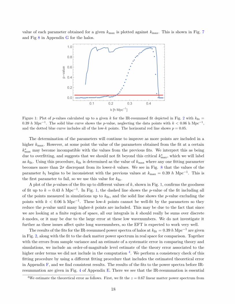
value of each parameter obtained for a given kmax is plotted against kmax. This is shown in Fig. 7

and Fig 8 in Appendix G for the halos.

0.1 0.2 0.3 0.4

0.0

0.2

0.4

0.6

0.8

1.0

k [h Mpc-1 ]

p-value

Figure 1: Plot of p-values calculated up to a given k for the IR-resummed fit depicted in Fig. 2 with kfit =

0.39 h Mpc−1. The solid blue curve shows the p-value, neglecting the data points with k < 0.06 h Mpc−1,

and the dotted blue curve includes all of the low-k points. The horizontal red line shows p = 0.05.

The determination of the parameters will continue to improve as more points are included in a

higher kmax. However, at some point the value of the parameters obtained from the fit at a certain

k∗max may become incompatible with the values from the previous fits. We interpret this as being

due to overfitting, and suggests that we should not fit beyond this critical k∗max, which we will label

as kfit. Using this procedure, kfit is determined as the value of kmax where any one fitting parameter

becomes more than 2σ discrepant from its lower-k values. We see in Fig. 8 that the values of the

parameter b1 begins to be inconsistent with the previous values at kmax = 0.39 h Mpc−1. This is

the first parameter to fail, so we use this value for kfit.

A plot of the p-values of the fits up to different values of k, shown in Fig. 1, confirms the goodness

of fit up to k = 0.43 h Mpc−1. In Fig. 1, the dashed line shows the p-value of the fit including all

of the points measured in simulations up to kfit, and the solid line shows the p-value excluding the

points with k < 0.06 h Mpc−1. These low-k points cannot be well-fit by the parameters so they

reduce the p-value until many higher-k points are included. This may be due to the fact that since

we are looking at a finite region of space, all our integrals in k should really be sums over discrete

k-modes, or it may be due to the large error at these low wavenumbers. We do not investigate it

further as these issues affect quite long wavenumbers, so the EFT is expected to work very well.

The results of the fits for the IR-resummed power spectra of halos at kfit = 0.39 h Mpc−1 are given

in Fig. 2, along with the fit to the dark matter power spectrum in real space for comparison. Together

with the errors from sample variance and an estimate of a systematic error in comparing theory and

simulations, we include an order-of-magnitude level estimate of the theory error associated to the

higher order terms we did not include in the computation 4. We perform a consistency check of this

fitting procedure by using a different fitting procedure that includes the estimated theoretical error

in Appendix F, and we find consistent results. The results of the fits to the power spectra before IR-

resummation are given in Fig. 4 of Appendix E. There we see that the IR-resummation is essential

4We estimate the theoretical error as follows. First, we fit the z = 0.67 linear matter power spectrum from

18

0.1 0.2 0.3 0.4 0.50.7

0.8

0.9

1.0

1.1

1.2

1.3

k [h Mpc-1]

PEFT,resum

/Psim,Halo

Figure 2: Results of the fits of the IR-resummed EFT power spectra at z = 0.67 to the power spectra of

halos and dark matter extracted from simulations. The halos have masses of M200 > 1× 1011 h−1M, with

a number density n = 3.8 · 10−2(hMpc−1 )3. The fits were performed in the k-range kmin = 0.01 h Mpc−1 to

kfit = 0.39 h Mpc−1 and resulted in the best-fit parameters b1 = 0.98± 0.01, b2 = 0.01± 2.73, b3 = −0.62±1.43, b4 = 0.58± 2.33, c

(δh)ct = (5.3± 4.7)

(kNL h−1Mpc

)2, cr,1 = (−14± 5)

(kM h−1Mpc

)2, cr,2 = (−0.69±

1.67)(kM h−1Mpc

)2, cε,1 = 0.76±14.74, cε,2 = (8.9±3.4)

(kM h−1Mpc

)2, cε,3 = (8.0±7.8)

(kM h−1Mpc

)2for the halos and c2s = (−0.61 ± 0.02)

(kNL h−1 Mpc

)2for the dark matter. The shaded regions show the

1σ error on the simulation data, which includes the error on the halo spectra from simulations described in

[44] and a 1% error that we add in quadrature to account for unknown systematic effects. The expected

theoretical error is given by the dotted lines.

for the fit, especially for the l = 2 mode which has oscillations of about 20% that are resummed. In

Fig. 2 the fits of the EFT to the halo power spectra fail at about the same wavenumber as the fit to

the dark matter power spectrum, which we expect from effective field theory. The bias parameters

determined by the fit for the IR-resummed halo power spectra along with their 1σ errors determined

CAMB as a piecewise power law [7, 8]:

P fit11 (k) = (2π)3

1k3NL

(kkNL

)nfor k > ktr

1k3NL

(kkNL

)nfor k < ktr .

(5.1)

Then, since the two-loop term scales approximately as P2−loop/P11 ∼ (k/kNL)2(3+n), we estimate the theo-

retical error on the dark matter power spectrum from neglecting the two-loop terms to be of order

∆P1−loop ∼ P2−loop ∼ 2π2P fit11 (k)

(k

kiNL

)2(3+ni)

, (5.2)

where kiNL, ni equals kNL, n for k > ktr and kNL, n for k < ktr, and the factor of 2π2 approximately

accounts for factors coming from integration. Since our universe does not have a true power-law spectrum

and since numerical factors are hard to estimate, the estimates for the theory error should be taken at the

order-of-magnitude level.

19

by the fitting procedure are 5:

b1 = 0.98± 0.01

b2 = 0.01± 2.73

b3 = −0.62± 1.43

b4 = 0.58± 2.33

c(δh)ct = (5.3± 4.7)

(kNL

h Mpc−1

)2

cr,1 = (−14± 5)

(kM

h Mpc−1

)2

cr,2 = (−0.69± 1.67)

(kM

h Mpc−1

)2

cε,1 = (0.76± 14.74)

cε,2 = (8.9± 3.4)

(kM

h Mpc−1

)2

cε,3 = (8.0± 7.8)

(kM

h Mpc−1

)2

. (5.3)

Note that the errors are quite correlated. We give the correlation matrix in Appendix G.

It is useful to provide a rough estimate of the scale kM suppressing the higher-derivative biases

of halos. We saw in Eq. (2.15) that the stochastic power spectrum, which renormalizes the single

halo contribution, can be estimated using the halo mass function. We can estimate the size of kM

by comparing the typical size of k−2M Pstoch, a higher-derivative correction to the stochastic power

spectrum, to the size of Pstoch:

1

k2M

∼

∫dM dn

dMM2

ρ2b

1k(M)2∫

dM dndM

M2

ρ2b

, (5.4)

where we have taken k(M) = 2π(4π3ρbM )1/3, the inverse size of a halo of mass M . This gives the

rough estimate kM ∼ 0.9hMpc−1 , which makes cr,1 and cr,2 order 1− 10, and the cε,i order one. Of

course this estimate should be taken at the order of magnitude level.

At this point, we should compare the size of the two-derivative stochastic terms to the size of the

“speed of sound” counter-terms to know whether it was consistent to include them. The cr,2 term is

the smallest “speed of sound” counter-term and the cε,3 term is the smallest stochastic counter-term.

The ratio of these terms is approximately

n−1W fµ2cε,3

µ4cr,2P11(k)∼ 400

P11(k), (5.5)

5The k0 stochastic term, which is parameterized by cε,1, must be positive because, after we subtract the UV

contribution for the diagrams of the 2-2 kind as we do, it represents the induced power spectrum from modes

into the non-linear regime. Thus, we have implemented the constraint cε,1 ≥ 0 in the fits. Since Mathematica

seems to us to have difficulty converging on the fits when the cε,1 ≥ 0 constraint is implemented, we start

the parameter values of b1, b2, b3, and cε,1 with the center values obtained in an unconstrained fit. b1 was

constrained to stay within ±6% of the center value, b2 and b3 were constrained to ±320%, and cε,1 was

bounded above by +1100% of the center value. The remaining parameters were left unconstrained.

20

which is order one or larger for k > 0.3. This means that the k2 stochastic terms are of the same

order of magnitude as the other k2 counter-terms, and must be included to be consistent. Thus,

we find that it was consistent to expand up to second order in derivatives in the power counting of

the stochastic term. The k4 terms we neglected in the derivative expansion of both the stochastic

and the “speed of sound” counter-term expressions are suppressed with respect to the ones we have

kept, but may become relevant at two-loop order.

This calculation is valid for the higher l modes as well, so in principle we could fit the l = 4, 6,8modes using the same ten free parameters, in analogy to the calculation done for dark matter in [29].

However, the higher-l modes are difficult to measure in simulations due to their small magnitude,

and they were not available for this analysis. All in all, we find that the EFT gives a good fit to

the simulated real-space halo power spectrum and the l = 0 and l = 2 modes of the redshift-space

halo power spectrum at z = 0.67 up to k = 0.43 h Mpc−1. Though extremely good, the actual

k-reach of the fit should be taken with care because, as noted for example in [23], it is possible that

the reach of the theory is somewhat overestimated when using just the one-loop expressions or not

extremely accurate data. Using for example more accurate data or the two-loop expressions, which

grow steeper at higher wavenumber, would allow a safer estimate of the k-reach. We plan to do this

in future work.

5.1 Fits to Galaxies

In this subsection we show that that we can also fit to a comparable level of accuracy the effective

theory to the power spectrum for a realistic model of galaxies in real space and redshift space 6.

This capability is indeed expected from the EFTofLSS point of view, because all biased tracers are

equal at a conceptual level, and they differ only for the size of the bias parameters (see [33] for a

discussion on how the k-reach is affected by different halo populations and how this might require

the addition of higher order terms in order to reach the same accuracy at a given wavenumber). The

fit to the power spectra of the vmpeakmodel of LRGs from [38] is given in Fig. 3. We find that the

theory agrees with the data to within a few percent up to k ∼ 0.43 h Mpc−1 (notice though that the

error bars for P2 are about 15% in the relevant region.). This fit has the same reach of the theory as

the fit to halos given in the main text, further demonstrating the consistency of the EFT. Note that

what looks like a failure of the fit around k ∼ 0.34 h Mpc−1 comes from the fact that the data for

P2 crosses zero there, so the ratio we are plotting diverges. This is just due to the choice of plotting

the ratio of the two curves rather than the two curves directly, and it is not a failure of the theory.

As we did for the halos, we perform a consistency check of our fitting procedure in Appendix F by

implementing a fitting procedure incorporating the estimated theoretical error, and find consistent

results.

6More precisely, at the highest wavenumbers where we fit, the errors for the real-space dark matter, the

real-space biased tracers, and the biased tracers monopole power spectra are less than 2%. Instead, the error

for the biased tracers power spectrum quadrupole is about 7% for the haloes and 15% for the vmpeakmodel

of LRGs.

21

0.0 0.1 0.2 0.3 0.4 0.5

0.7

0.8

0.9

1.0

1.1

1.2

1.3

k [h Mpc-1]

PEFT,resum

/Psim,vmpeak

0.0 0.1 0.2 0.3 0.4 0.5 0.6

0.0

0.2

0.4

0.6

0.8

1.0

k [h Mpc-1 ]

p-value

Figure 3: Left: Results of the fits of the EFT power spectra at z = 0.67 after IR-resummation to the power

spectra of LRGs in the vmpeaksample [38], which has a number density n = 3.9 · 10−4(hMpc−1 )3, and

dark matter extracted from simulations. The fits were performed in the k-range kmin = 0.01 h Mpc−1 to

kfit = 0.42 h Mpc−1 and resulted in the best-fit parameters b1 = 1.86 ± 0.04, b2 = 0.99 ± 7.59, b3 =

−4.5± 2.8, b4 = 0.68± 6.01, c(δh)ct = (0.69± 8.35)

(kNL h−1 Mpc

)2, cr,1 = (−30± 6)

(kM h−1 Mpc

)2, cr,2 =

(4.6±1.3)(kM h−1 Mpc

)2, cε,1 = 13±33, cε,2 = (30±12)

(kM h−1 Mpc

)2, cε,3 = (14±25)

(kM h−1 Mpc

)2for the LRGs and c2s = (−0.61 ± 0.02)

(kNL h−1 Mpc

)2for the dark matter. Preal is plotted in red, Pl=0 in

blue, Pl=2 in green, and PDM in orange. The shaded region shows the 1σ error on the simulation data, which

includes the error on the spectra from simulations described in [44] and a 1% error added in quadrature to

account for unknown systematics. The expected theoretical error is given by the dotted lines. Right: Plot of p-

values calculated up to a given k for the IR-resummed fit to the vmpeakpower spectra with kfit = 0.42 h Mpc−1.

The solid blue curve shows the p-value, neglecting the data points with k < 0.06 h Mpc−1, and the dotted

blue curve includes all of the low-k points. The horizontal red line shows p = 0.05.

6 Conclusion

In this paper, we extend the work done in the EFTofLSS to derive the power spectrum of dark

matter in redshift space [14, 29], and the power spectrum of halos in real space [13, 18, 33], in order

to calculate the power spectrum of halos in redshift space. We find that the power spectrum at one

loop is given in terms of ten parameters. The four bias parameters, as well as the first “speed of

sound” counter-term and stochastic counter-term have already been seen in the power spectrum of

halos in real space, and two of the redshift-space counter-terms appear already in the EFT of dark

matter in redshift space. In addition to these we find two novel higher-derivative stochastic bias

parameters that need to be included for the full study of halos in redshift space. We see that the

theory of biased tracers is extended to redshift space fairly easily, using only a few new integration

kernels, because we can treat the velocity divergence as a special species of halos. In addition, we

perform the IR-resummation of the halo power spectrum in redshift space, which follows directly

from [15]. In comparing to two populations of biased tracers, respectively with number density

n = 3.8 · 10−2(hMpc−1 )3 and n = 3.9 · 10−4(hMpc−1 )3, which are measured from simulations,

we find that the EFT agrees with the first two multipoles of the redshift-space halo power spectra

and the real-space matter and halo power spectra at z = 0.67 to within a few percent accuracy up

to k ' 0.43 h Mpc−1 7. We comment in the text on the fact that this actual value of the k-reach

7More precisely, at the highest wavenumbers where we fit, the errors for the real-space dark matter, the

real-space tracers, and the tracers monopole power spectra are less than 2%, while the error for the tracers

22

should be taken with care, and that, as pointed out in [33], it will depend at some level on the galaxy

population and the precision of the data. We also have excellent agreement with the BAO because

we do not have large residual oscillations in the IR-resummed power spectra.

In future work, we hope to be able to compare to higher multipoles, bispectra and to do so

at additional redshifts. This will allow us to test and understand more in detail how sample size

affects our results and to further check the consistency of the EFT approach, and in particular its

k-reach. We also plan to study how much each bias coefficient contributes to the fit, and, possibly,

in this way to reduce the number of parameters to be measured from simulations (or observations).

Finally, having the theory of biased tracers in redshift space means we can explore the cosmological

parameter constraints which can be achieved using the EFTofLSS framework on a realistic galaxy

sample at different redshifts, or, even better, directly to observations. We also hope to do this in

future work.

Acknowledgments

A.P. is partially supported by the Stanford Graduate Fellowship. L.S. is partially supported by DOE

Early Career Award DE-FG02-12ER41854. E.J. is supported by Fermi Research Alliance, LLC under

the U.S. Department of Energy under contract No. DEAC02-07CH11359. This work received partial

support from the U.S. Department of Energy under contract number DE-AC02-76SF00515. This

research made use of data from one of the Dark Sky Simulations, which were produced using an

INCITE 2014 allocation (M. Warren et al.) on the Oak Ridge Leadership Computing Facility at

Oak Ridge National Laboratory. We thank Sam Skillman, Mike Warren, Matt Turk and the Dark

Sky collaboration for making these data available.

A Halo kernels

The expressions for the basis operators c(n)i were found in [18] and corrected in [33]. We agree with

the corrections, and they are reproduced below. At first order,

c(1)δ,1 = 1 . (A.1)

At second order we have

c(2)δ,1 =

~q1 · ~q2

q21

c(2)δ,2 = F (2)(~q1, ~q2)− ~q1 · ~q2

q21

c(2)δ2,1

= 1

c(2)s2,1

=(~q1 · ~q2)2

q21q

22

− 1

3,

(A.2)

power spectrum quadrupole is about 7% for the haloes and 15% for the vmpeakmodel of LRGs.

23

and at third order,

c(3)δ,1 =

1

2

((~q1 · ~q2 + ~q1 · ~q3)

(~q2 + ~q3)2G(2)(~q2, q3) +

(~q1 · ~q2)(~q1 · ~q3 + ~q2 · ~q3)

q22q

23

)c

(3)δ,2 =

(~q1 · ~q3 + ~q2 · ~q3)

q22q

23

(F (2)(~q1, ~q2)q2

2 − ~q1 · ~q2

)c

(3)δ,3 = F (3)(~q1, ~q2, ~q3) +

(~q1 + ~q2) · ~q3

2q22q

23

(~q1 · ~q2 − 2F (2)(~q1, ~q2)q22)− ~q1 · (~q2 + ~q3)

2(~q2 + ~q3)2G(2)(~q2, ~q3)

c(3)δ2,1

= 2~q2 · ~q3

q23

c(3)δ2,2

= 2F (2)(~q1, ~q2)− 2~q2 · ~q3

q23

c(3)δ3,1

= 1

c(3)s2,1

= 2~q2 · ~q3

q23

((~q1 · ~q2)2

q21q

22

− 1

3

)c

(3)s2,2

= 2F (2)(~q1, ~q2)

(((~q1 + ~q2) · ~q3)2

(~q1 + ~q2)2q23

− 1

3

)− 2

(~q2 · ~q3)2

q23

((~q1 · ~q2)2

q21q

22

− 1

3

)c

(3)s3,1

= (9q21q

22q

23)−1

(9(~q1 · ~q2)(~q1 · ~q3)(~q2 · ~q3)− 3(~q1 · ~q3)2q2

2 − 3(~q1 · ~q2)q23 − 3(~q2 · ~q3)q2

1 + 2q21q

22q

23

)c

(3)st =

(G(2)(~q1, ~q2)− F (2)(~q1, ~q2)

)(((~q1 + ~q2) · ~q3)2

(~q1 + ~q2)2q23

− 1

3

)c

(3)ψ = G(3)(~q1, ~q2, ~q3)− F (3)(~q1, ~q2, ~q3) + 2F (2)(~q1, ~q2)

(F (2)(~q1 + ~q2, ~q3)−G(2)(~q1 + ~q2, ~q3)

)c

(3)δs2

=(~q1 · ~q2)2

q21q

22

− 1

3.

(A.3)

From [18, 33], the coefficients of the new basis c(A)i are related to the original coefficients c

(A)i as

c(A)δ,1 = c

(A)δ,1

c(A)δ,2(2) =

7

2c

(A)s2,1

+ c(A)δ,2

c(A)δ,2(3) =

7

2c

(A)s2,1

+ c(A)δ,2

c(A)δ,3 =

9

2c

(A)st,1 +

45

4c

(A)s3,1

+ c(A)δ,3 + 2c

(A)ψ,1

c(A)δ2,1(2)

= −17

6c

(A)s2,1

+ c(A)δ2,1

c(A)δ2,1(3)

= −17

6c

(A)s2,1

+ c(A)δ2,1

c(A)δ2,2

= −71

24c

(A)st,1 −

137

16c

(A)s3,1

+ c(A)δ2,2

+7

4c

(A)δs2,1− 55

42c

(A)ψ,1

c(A)s2,2

= −1

2c

(A)st,1 + c

(A)s2,2− 3

4c

(A)s3,1− 2

7c

(A)ψ,1

c(A)δ3,1

= −17

6c

(A)s2,1

+ c(A)δ2,1

. (A.4)

The choice of bias coefficients that make θh ≡ δθh are: cθhδ,1 = 1, cθhδ,2(2) = 2, cθhδ,2(3) = 2, cθhδ,3 =

24

3, cθhδ2,1(2)

= −1, cθhδ2,1(3)

= −1, cθhδ2,2

= −32 , c

θhs2,2

= 0, cθhδ3,1

= 1.The power spectrum will be computed using the symmetrized version of these kernels with the UV

part subtracted from the c(3)i , so the relevant kernels are c

(2)i (~k−~q, ~q)sym and c

(3)i (~k,−~q, ~q)UV−sub,sym:

c(2)δ,1(k, q, x)sym =

−2q3 + k3x+ 4kq2x− k2q − 2k2qx

2q(k2 + q2 − 2kqx)+ 1

c(2)δ,2(k, q, x)sym =

7q2 − 14kqx+ 5k2 + 2k2x2

7(k2 + q2 − 2kqx)− 1

c(2)δ2,1

(k, q, x)sym = 0 , (A.5)

and

c(3)δ,1(k, q, x)UV−sub,sym =

13

63

−7k6x2 + 28k4q2x2(x2 − 1)− 2q6(3 + 4x2) + k2q4(44x4 − 17x2 − 6)

42q2(k2 + q2 − 2kqx)(k2 + q2 − 2kqx)

c(3)δ,2(k, q, x)UV−sub,sym = − 4

63(3x2 − 1)

c(3)δ,3(k, q, x)UV−sub,sym = − 4

63

2q4(1− 3x2 + k4(3− 8x2 + x4 + k2q2(5− 22x2 + 25x4)))

(k2 + q2 + 2kqx)(k2 + q2 − 2kqx)

c(3)δ2,1

(k, q, x)UV−sub,sym = 0

c(3)δ2,2

(k, q, x)UV−sub,sym =8

63(3x2 − 1)

c(3)δ3,1

(k, q, x)UV−sub,sym = 0

c(3)s2,2

(k, q, x)UV−sub,sym =58q4(3x2 − 1)− k4(119− 267x2 + 90x4)− 2k2q2(74− 235x2 + 219x4)

189(k2 + q2 + 2kqx)(k2 + q2 − 2kqx),

(A.6)

where x =~k·~qkq .

B Degeneracy of halo bias parameters

We now turn to the explicit calculation of the halo kernels in real space. In the “basis of descendants”

of [18], which chooses the basis of linearly independent biases which gives priority to the various

operators that descend from a given one by the Taylor expansion of ~xfl, the density of a general halo

species A is given as

δ(n)A (~k) =

∫d3q1 . . . d

3qn K(n)A (~q1, . . . , ~qn)symδ

3D(~k − ~q1 . . .− ~qn)δ(1)(~q1) . . . δ(1)(~qn) , (B.1)

where these K(n)A,sym are the symmetrized versions of the following kernels:

K(1)A (~q1) = c

(A)δ,1 c

(1)δ,1(~q1) = c

(A)δ,1

K(2)A (~q1, ~q2) = c

(A)δ,1 c

(2)δ,1(~q1, ~q2) + c

(A)δ,2 c

(2)δ,2(~q1, ~q2) + c

(A)δ2,1

c(2)δ2,1

(~q1, ~q2)

K(3)A (~q1, ~q2, ~q3) = c

(A)δ,1 c

(3)δ,1(~q1, ~q2, ~q3) + c

(A)δ,2(3)c

(3)δ,2(~q1, ~q2, ~q3) + c

(A)δ,3 c

(3)δ,3(~q1, ~q2, ~q3)

+c(A)δ2,1(3)

c(3)δ2,1

(~q1, ~q2, ~q3) + c(A)δ2,2

c(3)δ2,2

(~q1, ~q2, ~q3) + c(A)δ3,1

c(3)δ3,1

(~q1, ~q2, ~q3)

+c(A)s2,2

c(3)s2,2

(~q1, ~q2, ~q3) , (B.2)

25

and where the c(n)i are the eight independent bias kernels given in Eq. (A.2) and Eq. (A.3). In terms

of these kernels, the power spectrum of halos in real space is

〈δA(~k)δA(~k)〉 = 〈δ(1)A (~k)δ

(1)A (~k)〉+ 〈δ(2)

A (~k)δ(2)A (~k)〉+ 2〈δ(1)

A (~k)δ(3)A (~k)〉

+〈δA(~k)δA(~k)〉ct + 〈δA(~k)δA(~k)〉ε

= (K(1)A )2P11(k) + 2

∫d3~q

(K

(2)A (~q,~k − ~q)sym

)2P11(|~k − ~q|)P11(q)

+6

∫d3~q K

(3)A (~q,−~q,~k)symK

(1)A P11(q)P11(k) + 〈δA(~k)δA(~k)〉ct

+〈δA(~k)δA(~k)〉ε . (B.3)

Explicitly, the symmetrized second order kernel for the halo density is:

K(2)δh

(k, q, x)sym =cδ,12q

−2q3 + k3x+ 4kq2x− k2q(1 + 2x2)

k2 + q2 − 2kqx

+cδ,2(2)

7

7q2 − 14kqx+ k2(5 + 2x2)

k2 + q2 − 2kqx+ cδ2,1(2) , (B.4)

which contains the three bias coefficients from the unsymmetrized kernel in Eq. (B.2).

Let us now turn to the more complicated third-order kernel. In the calculation, instead of using

K(3)A , we will actually use the UV-subtracted third-order kernel to make the integrals converge better.

This UV-subtraction is defined as

K(3)A (k, q, x)UV−sub = K

(3)A (k, q, x)− lim

qk→∞

K(3)A (k, q, x) , (B.5)

where the explicit expressions of the UV-subtracted c(3)i are given in Eq. (A.6). We are free to do

this because this change will be absorbed in a change of the counter-terms. Notice that in the q

integral of the third line of Eq. (B.3), K(3)A is the only term that has dependence on the angular

coordinate x, so we are free to perform the x integral on the kernel itself. After doing this integral

we find that the final third-order kernel is

K(3)δh

(k, q)UV−sub,sym =cδ,1

504k3q3

(−38k5q + 48k3q3 − 18kq5 + 9(k2 − q2)3 log

[k − qk + q

])+cδ,3 + 15cs2,2

756k3q5

(2kq(k2 + q2)(3k4 − 14k2q2 + 3q4) + 3(k2 − q2)4 log

[k − qk + q

]).

(B.6)

We see that after integration, K(3)A only contains three bias parameters, rather than the seven it

had in Eq. (B.2). This is because the momentum kernels multiplying the other four bias parameters

have integrated to zero. Of the three that remain, cδ,1 has already appeared in the second order

kernel, and cδ,3 and cs2,2 can be combined into one independent parameter. Thus we can define the

following four independent bias parameters at one-loop [18]:

b1 = cδ,1

b2 = cδ,2(2)

b3 = cδ,3 + 15cs2,2

b4 = cδ2,1(2) . (B.7)

26

It was only after the angular integral that the degeneracies in the c(n)i operators became fully

apparent. At higher loops, K(3)A will contract with kernels that have nontrivial angular dependence,

so the cancellations we encountered in Eq. (B.6) will not occur and the other four bias parameters

will become important. However, at one loop, the halo density power spectrum is fully described

by these four bias parameters plus the biased dark matter counter-term parameter, which we will

discuss in the main text along with the counter-terms from the transformation to redshift space.

Finally, the velocity divergence power spectrum is described by the following kernels

K(1)θh

(k, q, x)sym = 1

K(2)θh

(k, q, x)sym =k2(7kx− q(1 + 6x2))

14q(k2 + q2 − 2kqx)

K(3)θh

(k, q, x)UV−sub,sym =12k7q − 82k5q3 + 4k3q5 − 6kq7 + 3(k2 − q2)3(2k2 + q2) log

[k−qk+q

]504k3q5

,

(B.8)

with no additional free parameters. Now that we have the explicit expressions for the halo density

and velocity power spectra in real space, all that remains is to transform to redshift space.

C Redshift-space kernels

The contact terms in the redshift-space expansion generate new momentum kernels. The new terms

coming from the terms in brackets in Eq. (3.6) at second order are

δ(2)

[ ∂z∂2 θhδh]

(~k) =

∫~q1,~q2

(−iq1z

q21

)θ

(1)h (q1)δ

(1)h (q2)δ3

D(~k − ~q1 − ~q2)

=

∫~q1,~q2

(−iq1z

q21

)K

(1)θhK

(1)δhδ(1)(q1)δ(1)(q2)δ3

D(~k − ~q1 − ~q2)

δ(2)

[ ∂z∂2 θh

∂z∂2 θh]

(~k) =

∫~q1,~q2

(−iq1z

q21

)(−iq2z

q22

)θ

(1)h (q1)θ

(1)h (q2)δ3

D(~k − ~q1 − ~q2)

=

∫~q1,~q2

(−q1zq2z

q21q

22

)K

(1)θhK

(1)θhδ(1)(q1)δ(1)(q2)δ3

D(~k − ~q1 − ~q2) ,

(C.1)

27

and the new terms at third order are

δ(3)

[ ∂z∂2 θh

∂z∂2 θh

∂z∂2 θh]

(~k) =

∫~q1,~q2,~q3

(−iq1z

q21

)(−iq2z

q22

)(−iq3z

q23

)θ

(1)h (~q1)θ

(1)h (~q3)θ

(1)h (~q3)

δ3D(~k − ~q1 − ~q2 − ~q3)

=

∫~q1,~q2,~q3

(iq1zq2zq3z

q21q

22q

23

)K

(1)θhK

(1)θhK

(1)θhδ(1)(~q1)δ(1)(~q2)δ3

D(~k − ~q1 − ~q2 − ~q3)

δ(3)

[ ∂z∂2 θh

∂z∂2 θhδh]

(~k) =

∫~q1,~q2,~q3

(−iq1z

q21

)(−iq2z

q22

)θ

(1)h (q1)θ

(1)h (q2)δ

(1)h (q3)δ3

D(~k − ~q1 − ~q2 − ~q3)

=

∫~q1,~q2,~q3

(−q1zq2z

q21q

22

)K

(1)θhK

(1)θhK

(1)δhδ(1)(~q1)δ(1)(~q2)δ3

D(~k − ~q1 − ~q2 − ~q3)

δ(3)

[ ∂z∂2 θhδh]

(~k) =

∫~q1,~q2

(− iq2z

q22

δ(2)h (q1)θ

(1)h (q2)− iq1z

q21

θ(2)h (q1)δ

(1)h (q2)

)δ3D(~k − ~q1 − ~q2)

=

∫~q1,~q2,~q3

(− iq3z

q23

K(2)δh

(~q1, ~q2)K(1)θh− i(~q1 + ~q2)z

(~q1 + ~q2)2K

(2)θh

(~q1, ~q2)K(1)δh

)δ(1)(q1)δ(1)(~q2)δ(1)(~q3)δ3

D(~k − ~q1 − ~q2 − ~q3)

δ(3)

[ ∂z∂2 θh

∂z∂2 θh]

(~k) =

∫~q1,~q2

(−iq1,z

q21

)(−iq2,z

q22

)2θ

(2)h (q1)θ

(1)h (q2)δ3

D(~k − ~q1 − ~q2)

=

∫~q1,~q2,~q3

(−(~q1 + ~q2)zq3z

(~q1 + ~q2)2~q23

)2K

(2)θh

(~q1, ~q2)K(1)θhδ(1)(~q1)δ(1)(~q2)δ(1)(~q3)

δ3D(~k − ~q1 − ~q2 − ~q3) .

(C.2)

D The IR-safe integrand

Equal-time correlators in the EFT of LSS generically have IR divergences that cancel between

diagrams after integration. This cancellation is difficult to implement precisely in numerical calcu-

lations, so it is useful to find a formulation of the integrand that is manifestly IR-safe. This was

developed for dark matter correlators in [6], and we will extend it to halos in real space and redshift

space in this appendix.

For halos in real space, the extension is quite simple. It can be checked that all of the kernels

in Eq. (A.2) and Eq. (A.3) are finite in the limit q → 0 except for c(2)δ,1 and c

(3)δ,1 . These kernels come

into the power spectrum through the halo kernels K(2)A and K

(3)A as:

P(22)AB (k) = 2

∫d3~q K

(2)A (~q,~k − ~q)symK

(2)B (~q,~k − ~q)symP11(|~k − ~q|)P11(q)

P(13)AB (k) = 3

∫d3~q

(K

(3)A (~q,−~q,~k)symK

(1)B +K

(3)B (~q,−~q,~k)symK

(1)A

)P11(q)P11(k) . (D.1)

Since K(2)A comes into the power spectrum multiplied by K

(2)B , there are also sub-leading diver-

gences as q → 0 that are generated when the non-divergent kernels multiply c(2)δ,1 . From the explicit

expressions for the halo kernels given in Eq. (B.4) and Eq. (B.6), we find that the IR-divergent

28

contributions to P(22)AB are:

P(22)AB,IR(k) =

∫qk

d3q P11(q)P11(k)

(k2x2b

(A)1 b

(B)1

2q2− 7b

(A)1 b

(B)1 kx

q

+b(A)1 kx

q

(7b

(B)4 + b

(B)2

(5 + 2x2

))+b(A)1 kx

q

(7b

(B)4 + b

(B)2

(5 + 2x2

))). (D.2)

All of the terms proportional to q−1 are odd in the angular variable x, so we can make them IR-safe

by symmetrizing the integrand under the exchange ~q → −~q. In contrast, P(13)AB (k) is automatically

symmetric in x, and gives the following divergent term as q → 0:

P(13)AB,IR(k) = −

∫qk

d3qk2x2b

(A)1 b

(B)1

q2P11(q)P11(k) . (D.3)

The leading IR divergences from the integrands in Eq. (D.2) and Eq. (D.3) do not quite cancel.

However, the integrand of P(22)AB (k) has an additional divergence as ~k → ~q that we need to investigate.

Since we used the symmetrized kernel in Eq. (D.1), the integrand is symmetric under the exchange

~q → ~k − ~q. For any integrand f(~k, ~q) that has this symmetry, we can write the integral over ~q as:∫d3q f(~k, ~q) =

∫|~q|<|~k−~q|

d3q f(~k, ~q) +

∫|~q|>|~k−~q|

d3q f(~k, ~q)

=

∫|~q|<|~k−~q|

d3q f(~k, ~q) +

∫|~p|<|~k−~p|

d3p f(~k,~k − ~p) = 2

∫d3q f(~k, ~q)Θ(|~q| − |~k − ~q|) .

(D.4)

Thus, we can map the ~k → ~q divergence of P(22)AB into a q → 0 divergence. Implementing Eq. (D.4)

and symmetrizing with respect to ~q → −~q gives

P(22)AB,IR−safe(k) =

∫d3q

(K

(2)A (~q,~k − ~q)K(2)

B (~q,~k − ~q)P11(|~k − ~q|)P11(q)Θ(|~q| − |~k − ~q|)

+K(2)A (−~q,~k + ~q)K

(2)B (−~q,~k + ~q)P11(|~k + ~q|)P11(q)Θ(|~q| − |~k + ~q|)

).

(D.5)

Now in the ~q → 0 limit, the two terms in Eq. (D.5) give a factor of two that makes the leading

divergence of Eq. (D.2) cancel with Eq. (D.3), and the sub-leading divergences from Eq. (D.2) are

zero due to symmetrization. This makes the total integrand IR-safe.

When we go to redshift space, the new kernels K(n)h,r contain the real-space halo kernels K

(n)A ,

plus additional terms that are proportional to powers of µ and have new IR divergences. Let us first

consider P(13)h,r (k). We know that the only IR-divergent part of K

(3)A came from the kernel c

(3)δ,1 , so

none of the bias parameters other than b1 appear in the q → 0 limit. Indeed, in the q → 0 limit, we

find that the divergent part of P(13)h,r (k) is

P(13)h,r,IR(k) = −

∫qk

d3qπk2(b1 + fµ2)2(f2µ2(1− µ2) + x2(2 + fµ2(4 + f(3µ2 − 1))))

q2P11(q)P11(k) .

(D.6)

29

We turn now to P(22)h,r (k). Just as for the halos in real space, the terms in K

(2)h,r proportional

to b2, b3, and b4 are finite. However, since K(2)h,r comes into the power spectrum squared, we have

divergent terms proportional to these bias parameters that come from the non-IR-divergent part of

the halo kernel multiplying IR-divergent terms coming from the transformation to redshift space.

In the limit q → 0, all of these terms are odd in the angular variable x, so we can again symmetrize

in ~q → −~q to cancel them. After symmetrization, the q → 0 limit of P(22)h,r (k) is

P(22)h,r,IR(k) =

∫qk

d3qπk2(b1 + fµ2)2(f2µ2(1− µ2) + x2(2 + fµ2(4 + f(3µ2 − 1))))

2q2P11(q)P11(k)

= −1

2P

(13)h,r,IR(k) . (D.7)

Since K(2)h,r is symmetric in ~q → ~k − ~q, we can again use the trick in Eq. (D.4) to rewrite the

P(22)h,r,IR(k) integral in a form that cancels exactly with P

(13)h,r,IR(k). Thus we find that the IR-safe

integrand for halos in redshift space at one loop generalizes from the IR-safe integrand of dark

matter in real space, and entails rewriting 〈δh,rδh,r〉22 + 〈δh,rδh,r〉13 as follows:

〈δh,rδh,r〉22 + 〈δh,rδh,r〉13 =

∫d3q

(2(K

(2)h,r(~q,

~k − ~q)sym

)2P11(|~k − ~q|)P11(q)Θ(|~q| − |~k − ~q|)

+2(K

(2)h,r(−~q,~k + ~q)sym

)2P11(|~k + ~q|)P11(q)Θ(|~q| − |~k + ~q|)

+6(K

(3)h,r(~q,−~q,~k)symK

(1)h,r

)P11(q)P11(k)

). (D.8)

E More details of the IR-resummation

In this appendix we give the explicit procedure for the IR-resummation discussed in Section 4. The

IR-resummation procedure in redshift space involves computing the factor K0 defined in Eq. (4.4),

which is given explicitly by the expression

K0(~k, ~q) = exp

[−k

2

2X1(q)

(1 + 2fµ2 + f2µ2

)− k2

2Y1(q)

((k · q)2 + 2fµ(q · z)(k · q) + f2µ2(q · z)2

)],

where X1(q) and Y1(q) are the following functions of the linear halo power spectrum:

X1(q) =1

2π2

∫ ∞0

dk e(−k2/ΛIR)Phh(k)

(2

3− 2

j1(kq)

kq

)Y1(q) =

1

2π2

∫ ∞0

dk e(−k2/ΛIR)Phh(k)

(−2j0(kq) + 6

j1(kq)

kq

), (E.1)

and where the final answer is independent of the specific value of ΛIR as long as it includes all the

relevant modes that need to be resummed.

The authors of [29] noticed that due to the infinite radius of convergence of the exponential func-

tion, a Taylor series expansion can be used even for a non-infinitesimal argument of the exponential

as long as enough terms are kept to reach the desired precision. They found that for the one-loop

dark matter power spectrum it was sufficient to expand Eq. (E.1) to third order in µ2k2X1(q) and

to first order in k2Y1(q).

30

Using the same order of approximation as [29], we find that the halo power spectra in redshift

space can be resummed as follows:

P l,resumh,linear(k) =

∑l=0,2,4

∫d3q

[P l

′h,linear(q)M

(1)l,l′ (k) +

2l + 1

2e−

k2

2X1(q)

((1 +

k2

2X1(q)

)I0l,l′(k, q)

+k2

2f(2 + f)X1(q)I2

l,l′(k, q)

)P l

′h,linear(k)

]P l,resumh,1−loop(k) =

∑l=0,2,4,6,8

∫d3q

[P l

′h,1−loop(q)M

(0)l,l′ (k) +

2l + 1

2e−

k2

2X1(q)I0

l,l′(k, q)Pl′h,1−loop(k)

],

(E.2)

where M(n)l,l′ is given in Eq. (4.8) and

Ial,l′ =

∫ 1

−1dµ Pl(µ)Pl′(µ)µae−

k2

2X1(q)µ2f(2+f) . (E.3)

0.1 0.2 0.3 0.4 0.50.7

0.8

0.9

1.0

1.1

1.2

1.3

k [h Mpc-1]

PEFT/Psim,Halo

Figure 4: Results of the fits of the EFT power spectra at z = 0.67 before IR-resummation to the

power spectra of halos and dark matter extracted from simulations, which were performed in the k-

range kmin = 0.01 h Mpc−1 to kfit = 0.39 h Mpc−1 and resulted in the best-fit parameters b1 =

0.98± 0.01, b2 = 1.4± 1.9, b3 = −0.84± 0.88, b4 = −0.83± 1.63, c(δh)ct = (9.6± 3.0)

(kNL h−1Mpc

)2, cr,1 =

(−12 ± 4)(kM h−1Mpc

)2, cr,2 = (−0.45 ± 1.26)

(kM h−1Mpc

)2, cε,1 = −1.4 ± 10.7, cε,2 = (11 ±

2)(kM h−1Mpc

)2, cε,3 = (−7.1± 8.2)

(kM h−1Mpc

)2 for the halos and c2s = (−0.61± 0.02)(kNL h−1Mpc

)2for the dark matter. Preal is plotted in red, Pl=0 in blue, Pl=2 in green, and PDM in orange. The shaded re-

gion shows the 1σ error on the simulation data, which includes the error on the halo spectra from simulations

described in [44] and a 1% error added in quadrature to account for unknown systematics. The expected

theoretical error is given by the dotted lines.

The results of this resummation procedure are used for the fits in Fig. 2, while the non-IR-

resummed fits are given in Fig. 4. Comparing the two figures, we see that the IR resummation was

necessary to achieve a good fit to the simulation data, especially for the l = 2 mode.

31

F A Further Check of the Fitting Procedure

In this appendix, we implement a different fitting procedure that incorporates the estimated theo-

retical error in order to further test that we are not overfitting [31]. Since the theoretical error is

estimated only at the order of magnitude level, the results of this section should be taken more as

a reasonable consistency check rather than as an absolute check. In this procedure we use all of

the data up to k = 0.54 h Mpc−1, a point well past where the theory is expected to fail, and we

include the theoretical error described in footnote 4, added in quadrature to the data error and the

systematic error used for the fits in Section 5. The theoretical error is added in order to account

for the larger uncertainty at high k, so that these data can still be used in the fit without however

biasing the results. The results of this fitting procedure are given along with a plot of the p-value in

Fig. 5 for the halos and Fig. 6 for the vmpeaksample. We find that the parameters obtained in this

new fitting procedure agree with the parameters obtained in Section 5 to within 1σ for the halos

and 1.8σ for the LRGs (in this case only two parameters are beyond 1σ, one at 1.2σ and the other

at 1.8σ). Futhermore, the p-value plots in Fig. 5 and Fig. 6 indicate that the fits perform well up to

about the same k.

This procedure is somewhat uncertain, as the theory error is only known to within an order of

magnitude. However, it is encouraging that the results of this procedure are roughly consistent with

the fits performed in Section 5.

0.1 0.2 0.3 0.4 0.5 0.60.7

0.8

0.9

1.0

1.1

1.2

1.3

k [h Mpc-1]

PEFT,resum

/Psim,Halo

0.0 0.1 0.2 0.3 0.4 0.5 0.6

0.0

0.2

0.4

0.6

0.8

1.0

k [h Mpc-1 ]

p-value

Figure 5: Left: Results of the fits, including theoretical error in quadrature, of the EFT power spectra

at z = 0.67 after IR-resummation to the power spectra of halos [38], which has a number density n =

3.8 · 10−2(hMpc−1 )3, and dark matter extracted from simulations. The fits were performed in the k-range

0.01 h Mpc−1 to 0.54 h Mpc−1 and resulted in the best-fit parameters b1 = 0.98±0.01, b2 = 0.04±1.28, b3 =

0.06 ± 0.90, b4 = 0.56 ± 1.05, c(δh)ct = (6.2 ± 3.2)

(kNL h−1 Mpc

)2, cr,1 = (−15 ± 2)

(kM h−1 Mpc

)2, cr,2 =

(0.64±0.85)(kM h−1 Mpc

)2, cε,1 = 1.1±8.4, cε,2 = (4.6±1.0)

(kM h−1 Mpc

)2, cε,3 = (12±1)

(kM h−1 Mpc

)2for the halos and c2s = (−0.49 ± 0.01)

(kNL h−1 Mpc

)2for the dark matter. Preal is plotted in red, Pl=0 in

blue, Pl=2 in green, and PDM in orange. The shaded region shows the 1σ error on the simulation data, which

includes the error on the spectra from simulations described in [44] and a 1% error added in quadrature to

account for unknown systematics. The expected theoretical error is given by the dotted lines. Right: Plot of

p-values calculated up to a given k for the IR-resummed fit to the vmpeakpower spectra. The solid blue curve

shows the p-value, neglecting the data points with k < 0.06 h Mpc−1, and the dotted blue curve includes all

of the low-k points. The horizontal red line shows p = 0.05.

32

0.1 0.2 0.3 0.4 0.5 0.60.7

0.8

0.9

1.0

1.1

1.2

1.3

k [h Mpc-1]

PEFT,resum

/Psim,LRG

0.0 0.1 0.2 0.3 0.4 0.5 0.6

0.0

0.2

0.4

0.6

0.8

1.0

k [h Mpc-1 ]

p-value

Figure 6: Left: Results of the fits, including theoretical error in quadrature, of the EFT power spectra at z =

0.67 after IR-resummation to the power spectra of LRGs in the vmpeaksample [38], which has a number density

n = 3.9·10−4(hMpc−1 )3, and dark matter extracted from simulations. The fits were performed in the k-range

0.01 h Mpc−1 to 0.54 h Mpc−1 and resulted in the best-fit parameters b1 = 1.94±0.03, b2 = −0.08±9.06, b3 =

−0.81 ± 3.89, b4 = 1.7 ± 7.2, c(δh)ct = (9.9 ± 10)

(kNL h−1 Mpc

)2, cr,1 = (−39 ± 4)

(kM h−1 Mpc

)2, cr,2 =

(9.4± 1.4)(kM h−1 Mpc

)2, cε,1 = 4.5± 63.0, cε,2 = (18± 6)

(kM h−1 Mpc

)2, cε,3 = (35± 9)

(kM h−1 Mpc

)2for the LRGs and c2s = (−0.49 ± 0.01)

(kNL h−1 Mpc

)2for the dark matter. Preal is plotted in red, Pl=0 in

blue, Pl=2 in green, and PDM in orange. The shaded region shows the 1σ error on the simulation data, which

includes the error on the spectra from simulations described in [44] and a 1% error added in quadrature to

account for unknown systematics. The expected theoretical error is given by the dotted lines. Right: Plot of

p-values calculated up to a given k for the IR-resummed fit to the vmpeakpower spectra. The solid blue curve

shows the p-value, neglecting the data points with k < 0.06 h Mpc−1, and the dotted blue curve includes all

of the low-k points. The horizontal red line shows p = 0.05.

G Details of Parameter Fits

In this appendix we show the parameter plots used to determine the value of kfit for the halos, as

described in Section 5. We also include the correlation matrix of the parameters in Table 1.

References

[1] A. Schneider, R. Teyssier, D. Potter, J. Stadel, J. Onions, D. S. Reed, R. E. Smith,

V. Springel, F. R. Pearce, and R. Scoccimarro, Matter power spectrum and the challenge of

percent accuracy, JCAP 1604 (2016), no. 04 047, [arXiv:1503.05920].

[2] D. Baumann, A. Nicolis, L. Senatore, and M. Zaldarriaga, Cosmological Non-Linearities as an

Effective Fluid, JCAP 1207 (2012) 051, [arXiv:1004.2488].

[3] J. J. M. Carrasco, M. P. Hertzberg, and L. Senatore, The Effective Field Theory of

Cosmological Large Scale Structures, JHEP 09 (2012) 082, [arXiv:1206.2926].

[4] R. A. Porto, L. Senatore, and M. Zaldarriaga, The Lagrangian-space Effective Field Theory of

Large Scale Structures, JCAP 1405 (2014) 022, [arXiv:1311.2168].

[5] L. Senatore and M. Zaldarriaga, The IR-resummed Effective Field Theory of Large Scale

Structures, JCAP 1502 (2015), no. 02 013, [arXiv:1404.5954].

33

0.1 0.2 0.3 0.4

0.8

0.9

1.0

1.1

1.2

kmax [h Mpc-1]

b 1

0.1 0.2 0.3 0.4

-30

-20

-10

0

10

20

30

kmax [h Mpc-1]

b 2

0.1 0.2 0.3 0.4

-10

-5

0

5

kmax [h Mpc-1]

b 3

0.1 0.2 0.3 0.4-20

-10

0

10

20

kmax [h Mpc-1]

b 3

Figure 7: Parameter plots with 2σ errors for fits to halos up to a given kmax, for bias parameters b1, b2, b3,

and b4. The horizontal line shows the kmax at which b1 becomes incompatible with the earlier values.

Table 1: Correlation matrix for the bias coefficients of the halo sample.

b1 b2 b3 b4 c(δh)ct cr,1 cr,2 cε,1 cε,2 cε,3

b1 1. 0.34 -0.33 -0.3 -0.26 -0.09 -0.03 -0.68 -0.01 0.42

b2 0.34 1. -0.98 -1. -0.84 0.87 -0.77 -0.87 -0.77 -0.45

b3 -0.33 -0.98 1. 0.98 0.83 -0.81 0.71 0.9 0.65 0.36

b4 -0.3 -1. 0.98 1. 0.82 -0.88 0.77 0.86 0.78 0.5

c(δh)ct -0.26 -0.84 0.83 0.82 1. -0.81 0.91 0.65 0.72 0.14

cr,1 -0.09 0.87 -0.81 -0.88 -0.81 1. -0.91 -0.52 -0.91 -0.68

cr,2 -0.03 -0.77 0.71 0.77 0.91 -0.91 1. 0.45 0.86 0.39

cε,1 -0.68 -0.87 0.9 0.86 0.65 -0.52 0.45 1. 0.44 0.11

cε,2 -0.01 -0.77 0.65 0.78 0.72 -0.91 0.86 0.44 1. 0.63

cε,3 0.42 -0.45 0.36 0.5 0.14 -0.68 0.39 0.11 0.63 1.

[6] J. J. M. Carrasco, S. Foreman, D. Green, and L. Senatore, The 2-loop matter power spectrum

and the IR-safe integrand, JCAP 1407 (2014) 056, [arXiv:1304.4946].

34

0.1 0.2 0.3 0.4

-30

-20

-10

0

10

20

30

kmax [h Mpc-1]

c ct(δ

)k NL2

1hMpc

-12

0.1 0.2 0.3 0.4

-40

-20

0

20

40

kmax [h Mpc-1]

c˜r,1

k m2

1hMpc

-12

0.1 0.2 0.3 0.4

-10

-5

0

5

10

kmax [h Mpc-1]

c˜r,2

k m2

1hMpc

-12

0.1 0.2 0.3 0.4-60

-40

-20

0

20

40

60

kmax [h Mpc-1]

c ϵ,1

0.1 0.2 0.3 0.4

-10

0

10

20

30

kmax [h Mpc-1]

c ϵ,2

k m2

1hMpc

-12

0.1 0.2 0.3 0.4

-40

-20

0

20

40

kmax [h Mpc-1]

c ϵ,3

k m2

1hMpc

-12

Figure 8: Parameter plots with 2σ errors for fits to halos up to a given kmax, for counter-term parameters

c(δ)ct , cr,1, cr,2, cε,1, cε,2, and cε,3.

[7] J. J. M. Carrasco, S. Foreman, D. Green, and L. Senatore, The Effective Field Theory of

Large Scale Structures at Two Loops, JCAP 1407 (2014) 057, [arXiv:1310.0464].

[8] E. Pajer and M. Zaldarriaga, On the Renormalization of the Effective Field Theory of Large

Scale Structures, JCAP 1308 (2013) 037, [arXiv:1301.7182].

[9] S. M. Carroll, S. Leichenauer, and J. Pollack, Consistent effective theory of long-wavelength

cosmological perturbations, Phys. Rev. D90 (2014), no. 2 023518, [arXiv:1310.2920].

[10] L. Mercolli and E. Pajer, On the velocity in the Effective Field Theory of Large Scale

Structures, JCAP 1403 (2014) 006, [arXiv:1307.3220].

35

[11] R. E. Angulo, S. Foreman, M. Schmittfull, and L. Senatore, The One-Loop Matter Bispectrum

in the Effective Field Theory of Large Scale Structures, JCAP 1510 (2015) 039,

[arXiv:1406.4143].

[12] T. Baldauf, L. Mercolli, M. Mirbabayi, and E. Pajer, The Bispectrum in the Effective Field

Theory of Large Scale Structure, JCAP 1505 (2015), no. 05 007, [arXiv:1406.4135].

[13] L. Senatore, Bias in the Effective Field Theory of Large Scale Structures, JCAP 1511 (2015),

no. 11 007, [arXiv:1406.7843].

[14] L. Senatore and M. Zaldarriaga, Redshift Space Distortions in the Effective Field Theory of

Large Scale Structures, arXiv:1409.1225.

[15] M. Lewandowski, A. Perko, and L. Senatore, Analytic Prediction of Baryonic Effects from the

EFT of Large Scale Structures, JCAP 1505 (2015) 019, [arXiv:1412.5049].

[16] M. Mirbabayi, F. Schmidt, and M. Zaldarriaga, Biased Tracers and Time Evolution, JCAP

1507 (2015), no. 07 030, [arXiv:1412.5169].

[17] S. Foreman and L. Senatore, The EFT of Large Scale Structures at All Redshifts: Analytical

Predictions for Lensing, JCAP 1604 (2016) 033, [arXiv:1503.01775].

[18] R. Angulo, M. Fasiello, L. Senatore, and Z. Vlah, On the Statistics of Biased Tracers in the

Effective Field Theory of Large Scale Structures, JCAP 1509 (2015) 029, [arXiv:1503.08826].

[19] M. McQuinn and M. White, Cosmological perturbation theory in 1+1 dimensions, JCAP 1601

(2016), no. 01 043, [arXiv:1502.07389].

[20] V. Assassi, D. Baumann, E. Pajer, Y. Welling, and D. van der Woude, Effective theory of

large-scale structure with primordial non-Gaussianity, JCAP 1511 (2015) 024,

[arXiv:1505.06668].

[21] T. Baldauf, E. Schaan, and M. Zaldarriaga, On the reach of perturbative descriptions for dark

matter displacement fields, JCAP 1603 (2016), no. 03 017, [arXiv:1505.07098].

[22] T. Baldauf, M. Mirbabayi, M. Simonovic, and M. Zaldarriaga, Equivalence Principle and the

Baryon Acoustic Peak, Phys. Rev. D92 (2015), no. 4 043514, [arXiv:1504.04366].

[23] S. Foreman, H. Perrier, and L. Senatore, Precision Comparison of the Power Spectrum in the

EFTofLSS with Simulations, JCAP 1605 (2016) 027, [arXiv:1507.05326].

[24] T. Baldauf, L. Mercolli, and M. Zaldarriaga, Effective field theory of large scale structure at

two loops: The apparent scale dependence of the speed of sound, Phys. Rev. D92 (2015),

no. 12 123007, [arXiv:1507.02256].

[25] T. Baldauf, E. Schaan, and M. Zaldarriaga, On the reach of perturbative methods for dark

matter density fields, JCAP 1603 (2016), no. 03 007, [arXiv:1507.02255].

[26] D. Bertolini, K. Schutz, M. P. Solon, J. R. Walsh, and K. M. Zurek, Non-Gaussian

Covariance of the Matter Power Spectrum in the Effective Field Theory of Large Scale

Structure, arXiv:1512.07630.

36

[27] D. Bertolini, K. Schutz, M. P. Solon, and K. M. Zurek, The Trispectrum in the Effective Field

Theory of Large Scale Structure, arXiv:1604.01770.

[28] V. Assassi, D. Baumann, and F. Schmidt, Galaxy Bias and Primordial Non-Gaussianity,

JCAP 1512 (2015), no. 12 043, [arXiv:1510.03723].

[29] M. Lewandowski, L. Senatore, F. Prada, C. Zhao, and C.-H. Chuang, On the EFT of Large

Scale Structures in Redshift Space, arXiv:1512.06831.

[30] M. Cataneo, S. Foreman, and L. Senatore, Efficient exploration of cosmology dependence in

the EFT of LSS, arXiv:1606.03633.

[31] D. Bertolini and M. P. Solon, Principal Shapes and Squeezed Limits in the Effective Field

Theory of Large Scale Structure, arXiv:1608.01310.

[32] O. Hahn, R. E. Angulo, and T. Abel, The Properties of Cosmic Velocity Fields, Mon. Not.

Roy. Astron. Soc. 454 (2015), no. 4 3920–3937, [arXiv:1404.2280].

[33] T. Fujita, V. Mauerhofer, L. Senatore, Z. Vlah, and R. Angulo, Very Massive Tracers and

Higher Derivative Biases, arXiv:1609.00717.

[34] T. Baldauf, U. Seljak, L. Senatore, and M. Zaldarriaga, Galaxy Bias and non-Linear Structure

Formation in General Relativity, JCAP 1110 (2011) 031, [arXiv:1106.5507].

[35] T. Baldauf, U. Seljak, L. Senatore, and M. Zaldarriaga, Linear response to long wavelength

fluctuations using curvature simulations, JCAP 1609 (2016), no. 09 007, [arXiv:1511.01465].

[36] T. Lazeyras, C. Wagner, T. Baldauf, and F. Schmidt, Precision measurement of the local bias

of dark matter halos, JCAP 1602 (2016), no. 02 018, [arXiv:1511.01096].

[37] S. W. Skillman, M. S. Warren, M. J. Turk, R. H. Wechsler, D. E. Holz, and P. M. Sutter,

Dark Sky Simulations: Early Data Release, arXiv:1407.2600.

[38] E. Jennings, R. H. Wechsler, S. W. Skillman, and M. S. Warren, Disentangling redshift-space

distortions and non-linear bias using the 2D power spectrum, Mon. Not. Roy. Astron. Soc.

457 (2016), no. 1 1076–1088, [arXiv:1508.01803].

[39] P. McDonald and A. Roy, Clustering of dark matter tracers: generalizing bias for the coming

era of precision LSS, JCAP 0908 (2009) 020, [arXiv:0902.0991].

[40] R. Scoccimarro and J. Frieman, Loop corrections in nonlinear cosmological perturbation

theory, Astrophys. J. Suppl. 105 (1996) 37, [astro-ph/9509047].

[41] M. S. Warren, 2HOT: An Improved Parallel Hashed Oct-Tree N-Body Algorithm for

Cosmological Simulation, 2013. arXiv:1310.4502.

[42] P. S. Behroozi, R. H. Wechsler, and H.-Y. Wu, The Rockstar Phase-Space Temporal Halo

Finder and the Velocity Offsets of Cluster Cores, Astrophys. J. 762 (2013) 109,

[arXiv:1110.4372].

37

[43] B. V. Lehmann, Y.-Y. Mao, M. R. Becker, S. W. Skillman, and R. H. Wechsler, The

Concentration Dependence of the Galaxy-Halo Connection: Modeling Assembly Bias with

Abundance Matching, arXiv:1510.05651.

[44] H. A. Feldman, N. Kaiser, and J. A. Peacock, Power spectrum analysis of three-dimensional

redshift surveys, Astrophys. J. 426 (1994) 23–37, [astro-ph/9304022].

38