MA-108 Ordinary Differential Equations

M.K. Keshari

Department of MathematicsIndian Institute of Technology Bombay

Powai, Mumbai - 76

13th April, 2015D3 - Lecture 12

M.K. Keshari D3 - Lecture 12

Recall: Second Shifting Theorem:

L(u(t− a)g(t)) = e−sa L(g(t+ a))

Using this theorem, we can solve IVP with piecewisecontinuous forcing functions.

We introduced convolution of two functions f and g as

(f ∗ g)(t) =∫ t

0

f(τ)g(t− τ) dτ

Convolution Theorem:

L(f ∗ g) = F (s)G(s)

The convolution theorem provides a formula for solution of anIVP with unspecified forcing function.

M.K. Keshari D3 - Lecture 12

Examples

Example: Give a formula for the solution of the IVP.

y′′ + 2y′ + 2y = f(t), y(0) = a, y′(0) = b

Taking Laplace transform gives,

(s2 + 2s+ 2)Y (s) = F (s) + b+ as+ 2a. Therefore,

Y (s) =1

s2 + 2s+ 2F (s) +

b+ a+ a(s+ 1)

s2 + 2s+ 2

L−1(

1

s2 + 2s+ 2

)= e−t sin t,

Hence

y(t) =

∫ t

0

f(t− τ)e−τ sin τ dτ + e−t [(b+ a) sin t+ a cos t]

M.K. Keshari D3 - Lecture 12

Evaluating Convolution Integrals

Def. An integral of the form∫ t0f(τ)g(t− τ) dτ is called a

convolution integral.

Ex. Evaluate the integral

h(t) =

∫ t

0

(t− τ)5τ 7 dτ

We could do it by expanding the integrand. Let’s do it usingconvolution theorem.

h(t) = t5 ∗ t7, H(s) = L(t5)L(t7) =5! 7!

s6s8=

5! 7!

s14

Therefore,

h(t) = L−1(5! 7!

s14

)=

5! 7!

13!t13

M.K. Keshari D3 - Lecture 12

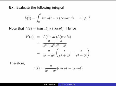
Ex. Evaluate the following integral

h(t) =

∫ t

0

sin a(t− τ) cos bτ dτ, |a| 6= |b|

Note that h(t) = (sin at) ∗ (cos bt). Hence

H(s) = L(sin at)L(cos bt)

=a

s2 + a2s

s2 + b2

=a

b2 − a2

(s

s2 + a2− s

s2 + b2

)Therefore,

h(t) =a

b2 − a2(cos at− cos bt)

M.K. Keshari D3 - Lecture 12

Volterra Integral Equations

An integral equation of the form

y(t) = f(t) +

∫ t

0

k(t− τ)y(τ) dτ

is called a Volterra integral equation. Here f(t) and k(t)are known functions and y is unknown.

We can solve them using convolution theorem.Taking Laplace transform, we get

Y (s) = F (s) +K(s)Y (s) =⇒ Y (s) =F (s)

1−K(s)

M.K. Keshari D3 - Lecture 12

Ex. Solve the integral equation

y(t) = 1 + 2

∫ t

0

e−2(t−τ)y(τ) dτ

Taking Laplace transform, we get

Y (s) =1

s+

2

s+ 2Y (s)

This gives Y (s)

(1− 2

s+ 2

)= Y (s)

s

s+ 2=

1

s

Y (s) =1

s+

2

s2=⇒ y(t) = 1 + 2t

M.K. Keshari D3 - Lecture 12

Additional Properties of Laplace Transform

Assume L(f(t)) is defined for s > s0, then

1 L(∫ t

0f(τ) dτ

)=F (s)

s, s > max{0, s0}.

2 L(tf(t)) = −F (1)(s), s > s0.

3 L

(f(t)

t

)=∫∞sF (s′)ds′, s > s0.

4 Assume f is piecewise continuous and of exponentialorder. Then(i) lims→∞ F (s) = 0, (ii) lims→∞ sF (s) is bounded.

5 Assume f and f ′ both are piecewise continuous and ofexponential order. Then lims→∞ sF (s) = f(0).

6 If f is piecewise continuous and periodic of period T ,

then L(f(t)) =1

1− e−sT∫ T0f(T )e−stdt, s > 0

M.K. Keshari D3 - Lecture 12

Theorem

If F (s) exists for s > s0, then

L

(∫ t

0

f(τ) dτ

)=F (s)

s, s > max{0, s0}

Proof.

L

(∫ t

0

f(τ)dτ

)= L(f ∗ 1) = L(f)L(1) =

F (s)

s

for s > max{0, s0}.

M.K. Keshari D3 - Lecture 12

Ex. Compute L−1(

1

sn+1

).

Since L(t) =1

s2, L(∫ t

0t dt)=

1

s3, i.e. L(t2) =

2

s3.

L(∫ t

0t2 dt

)=

2

s4=⇒ L(t3) =

3!

s4.

Proceeding by induction, we get L(tn) =n!

sn+1.

Ex. Find L−1(

1

s2(s2 + 1)

).

Since L(sin t) =1

s2 + 1,

L−1(

1

s2(s2 + 1)

)=

∫ t

0

∫ t

0

sin t dt

=

∫ t

0

(1− cos t) dt = t− sin t

M.K. Keshari D3 - Lecture 12

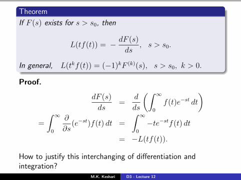
Theorem

If F (s) exists for s > s0, then

L(tf(t)) = − dF (s)

ds, s > s0.

In general, L(tkf(t)) = (−1)kF (k)(s), s > s0, k > 0.

Proof.

dF (s)

ds=

d

ds

(∫ ∞0

f(t)e−st dt

)=

∫ ∞0

∂

∂s(e−st)f(t) dt =

∫ ∞0

−te−stf(t) dt

= −L(tf(t)).

How to justify this interchanging of differentiation andintegration?

M.K. Keshari D3 - Lecture 12

Differentiation under the Integral sign

Suppose we need to differentiate the function

F (x) =

∫ b(x)

a(x)

f(x, t) dt

with respect to x. Assume a(x) and b(x) and their derivativesare continuous for x0 ≤ x ≤ x1 . Further f(x, t) and∂

∂xf(x, t) are continuous (in both t and x ) in some open

rectangle containing x0 ≤ x ≤ x1 and a(x) ≤ t ≤ b(x) .

Then for x0 ≤ x ≤ x1 :

d

dxF (x) = f(x, b(x)) b′(x)−f(x, a(x)) a′(x)+

∫ b(x)

a(x)

∂

∂xf(x, t) dt .

Search for “Leibniz Integral Rule”.M.K. Keshari D3 - Lecture 12

Ex. Find L−1(

s

(s2 + 4)2

).

If F (s) =1

s2 + 4, then f(t) =

1

2sin 2t. Hence

L(tf(t)) = −dF (s)ds

=2s

(s2 + 4)2.

Therefore, L−1(

s

(s2 + 4)2

)=

1

4t sin 2t.

Exercise. Find L−1(

s

(s2 + 4)3

).

M.K. Keshari D3 - Lecture 12

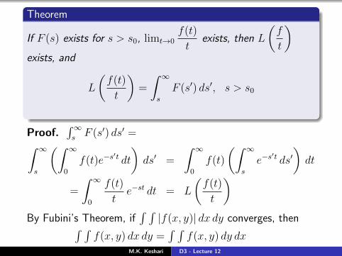
Theorem

If F (s) exists for s > s0, limt→0f(t)

texists, then L

(f

t

)exists, and

L

(f(t)

t

)=

∫ ∞s

F (s′) ds′, s > s0

Proof.∫∞sF (s′) ds′ =∫ ∞

s

(∫ ∞0

f(t)e−s′t dt

)ds′ =

∫ ∞0

f(t)

(∫ ∞s

e−s′t ds′

)dt

=

∫ ∞0

f(t)

te−st dt = L

(f(t)

t

)By Fubini’s Theorem, if

∫ ∫|f(x, y)| dx dy converges, then∫ ∫

f(x, y) dx dy =∫ ∫

f(x, y) dy dxM.K. Keshari D3 - Lecture 12

Ex. Find L−1(F (s)), where F (s) = ln

(s− as− b

), where a 6= b

are real numbers.

dF (s)

ds=

1

s− a− 1

s− b= G(s), say. If s0 = max {a, b}, then

g(t) = L−1(

1

s− a− 1

s− b

)= eat − ebt exists.

Since limt→0g(t)

t= limt→0

eat − ebt

t= a− b exists, we get

L

(g(t)

t

)=

∫ ∞s

G(s′) ds′ =

∫ ∞s

(1

s′ − a− 1

s′ − b

)ds′

= ln

(s′ − as′ − b

)|∞s = − ln

(s− as− b

)

Therefore, L−1(ln

(s− as− b

))= − g(t)

t=ebt − eat

t.

M.K. Keshari D3 - Lecture 12

Theorem

If f is piecewise continuous and of exponential order, then

(i) lims→∞ F (s) = 0, (ii) lims→∞ sF (s) <∞.

Proof. |f(t)| ≤Mes0t for t ≥ t0. Further we may assume|f(t)| ≤ K for t ∈ [0, t0]. Hence

|F (s)| =

∣∣∣∣∫ ∞0

f(t)e−st dt

∣∣∣∣ ≤ ∫ ∞0

|f(t)|e−st dt

=

∫ t0

0

|f(t)|e−st dt+∫ ∞t0

|f(t)|e−st dt

≤∫ t0

0

Ke−st dt+

∫ ∞t0

Me−(s−s0)t dt

= K1− e−st0

s+

M

s− s0, for all s > s0

=⇒ lims→∞

F (s) = 0, and lims→∞

sF (s) = K +M <∞

M.K. Keshari D3 - Lecture 12

Ex. Does there exist a function f(t) which is piecewisecontinuous and of exponential order, such that L(f(t)) = 1?No. Since then lims→∞ F (s) = 0.

May be there exist some function f(t) which is either notpiecewise continuous or not of exponential order, andL(f(t)) = 1. Answer is Yes. Dirac delta function or implusefunction has this property.

Exercise Find L−1 of (i)

(1

stanh s

), (ii) ln

(s2 + 1

s2 + s

), (iii)

ln

(1± 1

s2

).

Find if lims→∞ sF (s)→ f(0). If not, then state why.

M.K. Keshari D3 - Lecture 12

Theorem

Assume f and f ′ both are piecewise continuous and ofexponential order. Then

lims→∞

sF (s) = f(0).

Proof. Since

L(f ′(t)) = sL(f(t))− f(0)

Since f and f ′ both are piecewise continuous and ofexponential order, we get

lims→∞

L(f ′(t)) = 0, and lims→∞

sF (s) <∞

Therefore,lims→∞

sF (s) = f(0)

M.K. Keshari D3 - Lecture 12

Ex. Let f(t) = L−1(

1− s(5 + 3s)

s((s+ 1)2 + 1)

). Find f(0).

We can find f(t) by partial fraction. Hence we know that fand f ′ are continuous and of exponential order. Therefore,

f(0) = lims→∞

sF (s)

= lims→∞

1− s(5 + 3s)

((s+ 1)2 + 1)

= lims→∞

1− 5s− 3s2

s2 + 2s+ 2= −3

M.K. Keshari D3 - Lecture 12

Theorem

If f is piecewise continuous and periodic of period T , then

L(f(t)) =1

1− e−sT

∫ T

0

f(T )e−st dt, s > 0

Proof.

L(f(t)) =

∫ T

0

f(t)e−st dt+

∫ 2T

T

f(t)e−st dt+ . . .

=

∫ T

0

f(t)e−st dt+

∫ T

0

f(t+ T )e−s(t+T ) dt+ . . .

=

∫ T

0

f(t)e−st dt(1 + e−sT + e−2sT + . . .

)=

1

(1− e−sT )

∫ T

0

f(t)e−st dt , s > 0

M.K. Keshari D3 - Lecture 12

Ex. Find the Laplace transform of periodic function

f(t) =

{t, 0 ≤ t < 10, 1 ≤ t < 2

, f(t+ 2) = f(t)

L(f(t)) =1

(1− e−2s)

∫ 2

0

f(t)e−st dt

=1

(1− e−2s)

∫ 1

0

te−st dt

=1

(1− e−2s)

[te−st

−s|10 −

∫ 1

0

e−st

−sdt

]=

1

(1− e−2s)

[e−s

−s− 1

s2(e−s − 1)

]

M.K. Keshari D3 - Lecture 12