147
Ordinary Differential Equations A Linear Algebra Perspective (Version 1.75) L mg F(t) mg sin F(t) cos Todd Kapitula

Ordinary Differential Equations
A Linear Algebra Perspective(Version 1.75)
L
mg
F(t)
mg sin
F(t) cos
Todd Kapitula

Contents
Introduction . . . . . . . . . . . . . . . . . . . . . . . . . . . . . . . . . . . . . . . . . . . . . . . . . . . . . . . . . . . . . . . . . . . . . . . . . . . 1
1 Essentials of Linear Algebra . . . . . . . . . . . . . . . . . . . . . . . . . . . . . . . . . . . . . . . . . . . . . . . . . . . . . . . 71.1 Solving linear systems . . . . . . . . . . . . . . . . . . . . . . . . . . . . . . . . . . . . . . . . . . . . . . . . . . . . . . . . 8
1.1.1 Notation and terminology . . . . . . . . . . . . . . . . . . . . . . . . . . . . . . . . . . . . . . . . . . . . . 81.1.2 Solutions of linear systems . . . . . . . . . . . . . . . . . . . . . . . . . . . . . . . . . . . . . . . . . . . . 101.1.3 Solving by Gaussian elimination . . . . . . . . . . . . . . . . . . . . . . . . . . . . . . . . . . . . . . . 11
1.2 Vector algebra and matrix/vector multiplication . . . . . . . . . . . . . . . . . . . . . . . . . . . . . . . 181.2.1 Linear combinations of vectors . . . . . . . . . . . . . . . . . . . . . . . . . . . . . . . . . . . . . . . . 181.2.2 Matrix/vector multiplication . . . . . . . . . . . . . . . . . . . . . . . . . . . . . . . . . . . . . . . . . . . 19
1.3 Matrix algebra: addition, subtraction, and multiplication . . . . . . . . . . . . . . . . . . . . . . . 231.4 Sets of linear combinations of vectors . . . . . . . . . . . . . . . . . . . . . . . . . . . . . . . . . . . . . . . . . 25
1.4.1 Span of a set of vectors . . . . . . . . . . . . . . . . . . . . . . . . . . . . . . . . . . . . . . . . . . . . . . . . 251.4.2 Linear independence of a set of vectors . . . . . . . . . . . . . . . . . . . . . . . . . . . . . . . . 281.4.3 Linear independence of a set of functions . . . . . . . . . . . . . . . . . . . . . . . . . . . . . . 32
1.5 The structure of the solution . . . . . . . . . . . . . . . . . . . . . . . . . . . . . . . . . . . . . . . . . . . . . . . . . . 351.5.1 The homogeneous solution and the null space . . . . . . . . . . . . . . . . . . . . . . . . . . 351.5.2 The particular solution . . . . . . . . . . . . . . . . . . . . . . . . . . . . . . . . . . . . . . . . . . . . . . . . 38
1.6 Equivalence results . . . . . . . . . . . . . . . . . . . . . . . . . . . . . . . . . . . . . . . . . . . . . . . . . . . . . . . . . . . 421.6.1 A solution exists . . . . . . . . . . . . . . . . . . . . . . . . . . . . . . . . . . . . . . . . . . . . . . . . . . . . . . 421.6.2 A solution always exists . . . . . . . . . . . . . . . . . . . . . . . . . . . . . . . . . . . . . . . . . . . . . . . 431.6.3 A unique solution exists . . . . . . . . . . . . . . . . . . . . . . . . . . . . . . . . . . . . . . . . . . . . . . . 441.6.4 A unique solution always exists . . . . . . . . . . . . . . . . . . . . . . . . . . . . . . . . . . . . . . . . 45
1.7 Subspaces . . . . . . . . . . . . . . . . . . . . . . . . . . . . . . . . . . . . . . . . . . . . . . . . . . . . . . . . . . . . . . . . . . . 481.7.1 Vector spaces . . . . . . . . . . . . . . . . . . . . . . . . . . . . . . . . . . . . . . . . . . . . . . . . . . . . . . . . . 481.7.2 Subspaces and span . . . . . . . . . . . . . . . . . . . . . . . . . . . . . . . . . . . . . . . . . . . . . . . . . . . 481.7.3 The column space . . . . . . . . . . . . . . . . . . . . . . . . . . . . . . . . . . . . . . . . . . . . . . . . . . . . 50
1.8 Basis and dimension . . . . . . . . . . . . . . . . . . . . . . . . . . . . . . . . . . . . . . . . . . . . . . . . . . . . . . . . . . 521.8.1 Basis . . . . . . . . . . . . . . . . . . . . . . . . . . . . . . . . . . . . . . . . . . . . . . . . . . . . . . . . . . . . . . . . . 521.8.2 Dimension and rank . . . . . . . . . . . . . . . . . . . . . . . . . . . . . . . . . . . . . . . . . . . . . . . . . . 55
1.9 Inner-products and orthogonal bases . . . . . . . . . . . . . . . . . . . . . . . . . . . . . . . . . . . . . . . . . . 611.9.1 The inner-product on Rn . . . . . . . . . . . . . . . . . . . . . . . . . . . . . . . . . . . . . . . . . . . . . . 611.9.2 Orthonormal bases . . . . . . . . . . . . . . . . . . . . . . . . . . . . . . . . . . . . . . . . . . . . . . . . . . . . 631.9.3 Orthonormal bases and Fourier expansions . . . . . . . . . . . . . . . . . . . . . . . . . . . . 651.9.4 The Gram-Schmidt procedure . . . . . . . . . . . . . . . . . . . . . . . . . . . . . . . . . . . . . . . . . 661.9.5 Fourier expansions with trigonometric functions . . . . . . . . . . . . . . . . . . . . . . . 71
i
ii Contents
1.10 The matrix transpose, and two more subspaces . . . . . . . . . . . . . . . . . . . . . . . . . . . . . . . 751.10.1 Subspace relationships . . . . . . . . . . . . . . . . . . . . . . . . . . . . . . . . . . . . . . . . . . . . . . . . 761.10.2 Least squares . . . . . . . . . . . . . . . . . . . . . . . . . . . . . . . . . . . . . . . . . . . . . . . . . . . . . . . . . 79
1.11 Matrix algebra: the inverse of a square matrix . . . . . . . . . . . . . . . . . . . . . . . . . . . . . . . . . 821.12 The determinant of a square matrix . . . . . . . . . . . . . . . . . . . . . . . . . . . . . . . . . . . . . . . . . . . 861.13 Linear algebra with complex-valued numbers, vectors, and matrices . . . . . . . . . . . 921.14 Eigenvalues and eigenvectors . . . . . . . . . . . . . . . . . . . . . . . . . . . . . . . . . . . . . . . . . . . . . . . . . 98
1.14.1 Characterization of eigenvalues and eigenvectors . . . . . . . . . . . . . . . . . . . . . . . 981.14.2 Properties . . . . . . . . . . . . . . . . . . . . . . . . . . . . . . . . . . . . . . . . . . . . . . . . . . . . . . . . . . . . 1051.14.3 Eigenvectors as a basis, and Fourier expansions . . . . . . . . . . . . . . . . . . . . . . . . 106
1.15 Case studies . . . . . . . . . . . . . . . . . . . . . . . . . . . . . . . . . . . . . . . . . . . . . . . . . . . . . . . . . . . . . . . . . . 1111.15.1 Voter registration . . . . . . . . . . . . . . . . . . . . . . . . . . . . . . . . . . . . . . . . . . . . . . . . . . . . . 1111.15.2 Discrete SIR model . . . . . . . . . . . . . . . . . . . . . . . . . . . . . . . . . . . . . . . . . . . . . . . . . . . . 1141.15.3 Northern spotted owl . . . . . . . . . . . . . . . . . . . . . . . . . . . . . . . . . . . . . . . . . . . . . . . . . 118
Group projects . . . . . . . . . . . . . . . . . . . . . . . . . . . . . . . . . . . . . . . . . . . . . . . . . . . . . . . . . . . . . . . . . . . . 123
MATLAB support . . . . . . . . . . . . . . . . . . . . . . . . . . . . . . . . . . . . . . . . . . . . . . . . . . . . . . . . . . . . . . . . . . . . . . 129
Answers to selected exercises . . . . . . . . . . . . . . . . . . . . . . . . . . . . . . . . . . . . . . . . . . . . . . . . . . . . . . . . . . 137References . . . . . . . . . . . . . . . . . . . . . . . . . . . . . . . . . . . . . . . . . . . . . . . . . . . . . . . . . . . . . . . . . . . . . . . . 141
Index . . . . . . . . . . . . . . . . . . . . . . . . . . . . . . . . . . . . . . . . . . . . . . . . . . . . . . . . . . . . . . . . . . . . . . . . . . . . . . . . . . 143
Introduction
ch:intro
This book arose from lecture notes that I began to develop in 2010-2011 for a first course in or-dinary differential equations (ODEs). At Calvin College the students in this course are primarilyengineers. In our engineering program it is generally the case that the only (formal) linear al-gebra the students see throughout their undergraduate career is what is presented in the ODEcourse. This is not unusual, as the ABET Accreditation Criteria of 2012-13 do not explicitlyrequire a course devoted to the study of linear algebra. Since, in my opinion, the amount ofmaterial on linear algebra covered in, e.g., the classical text of Boyce and DiPrima [10], is in-sufficient if that is all you will see in your academic career, I found it necessary to supplementwith notes on linear algebra of my own design. Eventually, it became clear that in order tohave a seamless transition between the linear algebra and ODEs, there needed to be one text.This is not a new idea; for example, two recent texts which have a substantive linear algebracomponent are by Boelkins et al. [7] and Edwards and Penney [16].
Because there is a substantive linear algebra component in this text, I - and more importantly,the students - found it to be much easier later in the text when discussing the solutions of linearsystems of ODEs to focus more on the ODE aspects of the problems, and less on the underlyingalgebraic manipulations. I have found that by doing the linear algebra first, it allowed me tomore extensively and deeply explore linear systems of ODEs. In particular, it is possible to domuch more interesting examples and applications. I believe that this inclusion of more modelingand model analysis is extremely important; indeed, it is precisely what is recommended inthe 2013 report by the National Academy of Sciences on the current state, and future, of themathematical sciences.
The applications presented in this text are labeled “Case Studies”. I chose this moniker be-cause I wanted to convey to the reader that in solving particular problems we were going todo more than simply find a solution; instead, we were going to take time to determine whatthe solution was telling us about the dynamical behaviour for the given physical system. Thereare 18 case studies presented herein. Some are classical - e.g., damped mass-spring systems,mixing problems (compartment models) - but several are not typically found in a text such asthis. Such examples include a discrete SIR model, a study of the effects on the body of leadingestion, strongly damped systems (which can be recast as a singular perturbation problem),and a (simple) problem in the mathematics of climate. It is (probably) not possible to presentall of these case studies in a one-semester course. On the other hand, the large number allowsthe instructor to choose a subset which will be of particular interest to his/her class.
The book is formatted as follows. In Chapter 1 we discuss not only the basics of linear algebrathat will be needed for solving systems of linear ordinary differential equations, e.g., Gaussianelimination, matrix algebra, and eigenvalues/eigenvectors, but we discuss such foundationalmaterial as subspaces, dimension, etc. While the latter material is not necessary to solve ODEs,
1
2 Introduction
I find that this is a natural time to introduce students to these more abstract linear algebraconcepts. Moreover, since linear algebra is such foundational material for a mathematical un-derstanding of all of the sciences, I feel that it is essential that the students’ learn as much asthey reasonably can in the short amount of time that is available. It is typically the case that thematerial in Chapter 1 can be covered in about 15-18 class periods. Primarily because of timeconstraints, when presenting this material I focus primarily on the case of the vector space Rn.The culminating section in the chapter is that on eigenvalues and eigenvectors. Here I espe-cially emphasize the utility of writing a given vector as a linear combination of eigenvectors.The closing section considers the large-time behavior associated with three discrete dynamicalsystems. If the reader and/or instructor wishes to have a supplementary text for this chapter,the book by Hefferon [23] is an excellent companion. Moreover , the PDF can be had for free athttp://joshua.smcvt.edu/linearalgebra/.
Once the linear algebra has been mastered, we begin the study of ODEs by first solvingscalar first-order linear ODEs in ??. We briefly discuss the general existence/uniqueness the-ory, as well as the numerical solution. When solving ODEs numerically, we use the MATLABprograms dfield8.m and pplane8.m developed by J. Polking. These MATLAB programs haveaccompanying Java applets:
• DFIELD: http://math.rice.edu/∼dfield/dfpp.html• PPLANE: http://math.rice.edu/∼dfield/dfpp.html.
My experience is that these software tools are more than sufficient to numerically solve theproblems discussed in this class. We next construct the homogeneous and particular solutionsto the linear problem. In this construction we do three things:
(a) derive and write the homogeneous solution formula in such a way that the later notionof a homogeneous solution being thought of as the product of a matrix-valued solutionand a constant vector is a natural extension
(b) derive and write the variation-of-parameters solution formula in such a manner that theideas easily generalize to systems
(c) develop the technique of undetermined coefficients.
The chapter closes with a careful analysis of the one-tank mixing problem under the assump-tion that the incoming concentration varies periodically in time, and a mathematical financeproblem . The idea here is to:
(a) show the students that understanding is not achieved with a solution formula; instead, itis necessary that the formula be written “correctly” so that as much physical informationas possible can be gleaned from it
(b) introduce the students to the ideas of amplitude plots and phase plots(c) set the students up for the later analysis of the periodically forced mass-spring.
As a final note, in many (if not almost all) texts there is typically in this chapter an extensivediscussion on nonlinear ODEs. I chose to provide only a cursory treatment of this topic at theend of this book because of:
(a) my desire for my students to understand and focus on linearity and its consequences(b) the fact that we at Calvin College teach a follow-up course on nonlinear dynamics using
the wonderful text by Strogatz [40].
In ?? we study systems of linear ODEs. We start with five physical examples, three of whichare mathematically equivalent in that they are modeled by a second-order scalar ODE. We showthat nth-order scalar ODEs are equivalent to first-order systems, and thus (hopefully) convincethe student that it is acceptable to skip (for the moment) a direct study of these higher-order

Introduction 3
scalar problems. We almost immediately go the case of the homogeneous problem being con-stant coefficient, and derive the homogeneous solution via an expansion in terms of eigenvec-tors. From a pedagogical perspective I find (and my students seem to agree) this to be a naturalway to see how the eigenvalues and eigenvectors of a matrix play a key role in the construc-tion of the homogeneous solution, and in particular how using a particular basis may greatlysimplify a given problem. Moreover, I find that this approach serves as an indirect introduc-tion to the notion of Fourier expansions, which is of course used extensively in a successorcourse on linear partial differential equations. After we construct the homogeneous solutionswe discuss the associated phase plane. As for the particular solutions we mimic the discussionof the previous chapter and simply show what few modifications must be made in order forthe previous results to be valid for systems. My experience has been that the manner in whichthings were done in the previous chapter helps the student to see that it is not the case we arelearning something entirely new and different, but instead we are just expanding on an alreadyunderstood concept. The chapter closes with a careful analysis of three problems: a two-tankmixing problem in which the incoming concentration into at one of the tanks is assumed tovary periodically in time, a study of the effect of lead ingestion, and an SIR model associatedwith zoonotic (animal-to-human) bacterial infections. As in the previous chapter the goal is tonot only construct the mathematical solution to the problem, but to also understand how thesolution helps us to understand the dynamics of the given physical system.
In ?? we solve higher-order scalar ODEs. Because all of the theoretical work has already beendone in the previous chapter, it is not necessary to spend too much time on this particular task.In particular, there is a relatively short presentation as to how one can use the systems theoryto solve the scalar problem. The variation of parameters formula is not re-derived; instead, it isjust presented as a special case of the formula for systems. We conclude with a careful study ofseveral problems: the undamped and damped mass-spring systems, a (linear) pendulum drivenby a constant torque, a couple mass-spring system, and the vibrations of a beam. The last studyintroduces the separation of variables technique for solving linear PDEs. Nice illustrative Javaapplets for the mass-spring problems are:
• Forced and damped oscillations of a spring pendulum:http://www.walter-fendt.de/ph14e/resonance.htm
• Coupled oscillators:http://www.lon-capa.org/%7emmp/applist/coupled/osc2.htm.
There are also illustrative movies which are generated by MATLAB.In ?? we solve scalar ODEs using the Laplace transform. The focus here is to solve only
those problems for which the forcing term is a linear combination of Heaviside functions anddelta functions. In my opinion any other type of forcing term can be more easily handled witheither the method of undetermined coefficients or variation of parameters. Moreover, we focuson using the Laplace transform as a method to find the particular solution, with the understand-ing that we can find the homogeneous solution using the ideas and techniques from previouschapters. In order to simplify the calculations, we assume that when finding the particular so-lution there is zero initial data. Because of the availability of WolframAlpha, we spend littletime on partial fraction expansions and the inversion of the Laplace transform. The subse-quent case studies are somewhat novel. We start with finding a way to stop the oscillationsfor an undamped mass-spring system. For our second problem, we study a one-tank mixingproblem in which in the incoming concentration varies periodically in time. The injection strat-egy is modeled as an infinite sum of delta functions. Our last case study involves the analysisof a strongly damped mass-spring problem. We show that this system can be thought of asa singular perturbation problem which is (formally) mathematically equivalent to a one-tankmixing problem. We finish the discussion of the Laplace transform with the engineering appli-

4 Introduction
cations of the transfer function, the manner in which the poles of the transfer function effectthe dynamics of the homogeneous solution. We show that the convolution integral leads to avariation-of-parameters formula for the particular solution.
In ?? we cover topics which are not infrequently discussed if time permits: separation ofvariables, phase line analysis, and series solutions. Each topic is only briefly touched upon, butenough material is presented herein for the student to get a good idea of what each one is about.For the latter two topics I present case studies which could lead to a more detailed examinationof the topic (using outside resources) if the student and/or instructor wishes.
Almost every section concludes with a set of homework problems. Moreover, there is asection at the end of each of Chapter 1, ??, ??, and ?? which is labeled Group Projects. Theproblems contained in these sections are more challenging, and I find it to be the case thatthe students have a better chance of understanding and solving them if they work together ingroups of 3-4 people. My experience is that the students truly enjoy working on these problems,and they very much appreciate working collaboratively. I typically assign 1-2 of these types ofproblems per semester.
As of the current edition relatively few of the homework problems have attached to them asolution. My expectation is that many, if not most, students will find this lack of solved problemstroubling. Two relatively cheap (potentially supplemental) texts which address this issue areLipschutz and Lipson [29] for the linear algebra material and Bronson and Costa [11] for theODE material. Of course, other books, e.g., [6, 13, 20, 35], can be found simply by going to thelibrary and looking there through the (perhaps) dozens of appropriate books.
Throughout this text we expect the students to use a CAS to do some of the intermediatecalculations. Herein we focus upon WolframAlpha (http://www.wolframalpha.com/). Thereare several advantages to using this particular CAS:
(a) it is not necessary to learn a programming language to use it(b) the commands are intuitive(c) it is easily accessible(d) it is free (as of June, 2014).
I appreciate that the interested reader and/or instructor can do much more with Mathematica,Maple, Sage, etc. However, there is currently no universal agreement as to which package is bestto use (even within my department!), and I do not want to limit this text to a particular system.Moreover, my goal here is to focus more on using the software to solve a given problem, andnot on the programming necessary to use the particular CAS. My expectation is that interestedstudents who have some experience with a particular CAS will quickly learn how to do whatthey want to do with it.
In this text we do not use this software to completely solve a given problem, as it is im-portant that the student thoroughly understand what intermediate calculations are needed inorder to solve the problem. The idea here is that the CAS can be used to remove some of thecomputational burden associated with solving a problem. A screenshot is provided in the textfor most of the calculations, so it should be easy for the student to replicate. In addition, thereis a brief section at the end of the text which shows how one can use MATLAB to performmany of the intermediate calculations. The particular scripts are provided on my web page athttp://www.calvin.edu/∼ tmk5/courses/m231/S14/.
In the ODE portion of this text we attempt to emphasize the idea that the interesting thing isnot necessarily the mathematical solution of a given mathematical problem, but what it is thatthe solution tells you about the physical problem being modeled. The (extremely) easy-to-useCAS generally does a reasonable job of solving a given mathematical equation, but it is not quiteas helpful when interpreting a solution.

Introduction 5
The electronic version of this book is embedded with hyperlinks (both internal and external),and they are marked in blue text. It is my hope that these links make it easier to navigate thebook; in particular, it should be the case that it is easier (and quicker than a paper version!) forthe reader to reference previous results, e.g., to recall a result on page 69 while reading page 113.The book does include a minimal index. It mostly provides the first page at which a particularterm is mentioned. In particular, it does provide the page for which each term is first defined.Since it is expected that this book will be primarily used in an electronic format, this potentialdrawback is easily overcome via a “find” command.
I am indebted to Kate Ardinger, Tom Jager, Jeff Humpherys, Michael Kapitula, Keith Promis-low, Thomas Scofield, Matt Walhout, and anonymous reviewers for discussions about, and acareful reading of, this manuscript. The implementation of their suggestions and commentsgreatly improved the text.
For the glory of the most high God alone,And for my neighbour to learn from.
J.S. Bach


Chapter 1Essentials of Linear Algebra
ch:linalg
Mathematics is the art of reducing any problem to linear algebra.- William Stein
To many, mathematics is a collection of theorems. For me, mathematics is a collectionof examples; a theorem is a statement about a collection of examples and the purposeof proving theorems is to classify and explain the examples . . .- John Conway
The average college student knows how to solve two equations in two unknowns in anelementary way: the method of substitution. For example, consider the system of equations
2x+ y = 6, 2x+ 4y = 5.
Solving the first equation for y gives y = 6−2x, and substituting this expression into the secondequation yields
2x+ 4(6− 2x) = 5 x =19
6.
Substitution into either of the equations gives the value of y; namely, y = −1/3. For systems ofthree or more equations this algorithm is algebraically unwieldy. Furthermore, it is inefficient,as it is often the case not very clear as to which variable(s) should be substituted into whichequation(s). Thus, at the very least, we should develop an efficient algorithm for solving largesystems of equations. Perhaps more troubling (at least to the mathematician!) is the fact thatthe method of substitution does not yield any insight into the structure of the solution set. Ananalysis and understanding of this structure is the topic of linear algebra. As we will see, notonly will we gain a much better understanding of how to solve linear algebraic systems, but byconsidering the problem more abstractly we will better understand how to solve linear systemsof ordinary differential equations (ODEs).
This chapter is organized in the following manner. We begin our discussion of linear sys-tems of equations by developing an efficient solution algorithm: Gaussian elimination. We thenconsider the problem using matrices and vectors, and spend considerable time and energy try-ing to understand the solution structure via these objects. In particular, we show that that thesolution is composed of two pieces. One piece intrinsically associated with the matrix alone,and the other piece reflects an interaction between the matrix and nonhomogeneous term. Weconclude the chapter by looking at special vectors associated with square matrices: the eigen-
7
8 1 Essentials of Linear Algebra
vectors. These vectors have the special algebraic property that the matrix multiplied by aneigenvector is simply a scalar multiple of that eigenvector (this scalar is known as the associ-ated eigenvalue). As we will see, the eigenvalues and eigenvectors are the key objects associatedwith a matrix that allow us to easily and explicitly write down and understand the solution toa linear dynamical systems (both discrete and continuous).
1.1 Solving linear systems
1.1.1 Notation and terminology
A linear equation in n variables is an algebraic equation of the form
a1x1 + a2x2 + · · ·+ anxn = b. (1.1.1) e:121
The (possibly complex-valued) numbers a1, a2, . . . , an are the coefficients, and the unknownsto be solved for are the variables x1, . . . , xn. The variables are also sometimes called un-knowns. An example in two variables is
2x1 − 5x2 = 7,
and an example in three variables is
x1 − 3x2 + 9x3 = −2.
A system of linear equations is a collection of m linear equations (1.1.1), and can be written as
a11x1 + a12x2 + · · ·+ a1nxn = b1
a21x1 + a22x2 + · · ·+ a2nxn = b2
......
am1x1 + am2x2 + · · ·+ amnxn = bm.
(1.1.2) e:122
The coefficient ajk is associated with the variable xk in the jth equation. An example of twoequations in three variables is
x1 − 4x2 = 6
3x1 + 2x2 − 5x3 = 2.(1.1.3) e:123
Until we get to our discussion of eigenvalues and eigenvectors in Chapter 1.14, we willassume that the coefficients and variables are real numbers, i.e., ajk, xj ∈ R. This isdone solely for the sake of pedagogy and exposition. It cannot be stressed too much,however, that everything we do preceding Chapter 1.14 still works even if we removethis restriction, and we allow these numbers to be complex (have nonzero imaginarypart).
When there is a large number of equations and/or variables, it is awkward to write down alinear system in the form of (1.1.2). It is more convenient instead to use a matrix formulation.

1.1 Solving linear systems 9
A matrix is a rectangular array of numbers with m rows and n columns, and such a matrix issaid to be an m× n (read “m by n”) matrix. If m = n, the matrix is said to be a square matrix.
For an m × n matrix with real entries we will say A ∈ Mm×n(R). If the matrix issquare, i.e., m = n, then we will write A ∈ Mn(R). The R is there to emphasize thatall of the entries are real numbers. If the entries are allowed to be complex, we willwrite A ∈Mm×n(C), or A ∈Mn(C).
The coefficient matrix for the linear system (1.1.2) is given by
A =
a11 a12 · · · a1na21 a22 · · · a2n
...... · · ·
...am1 am2 · · · amn
, (1.1.4) e:124
and the coefficient ajk , which is associated with the variable xk in the jth equation, is in thejth row and kth column. For example, the coefficient matrix for the system (1.1.3) is given by
A =
(1 −4 03 2 −5
)∈M2×3(R),
witha11 = 1, a12 = −4, a13 = 0, a21 = 3, a22 = 2, a23 = −5.
A vector, say v ∈Mm×1(R), is a matrix with only one column. A vector is sometimes called acolumn vector or m-vector. To clearly distinguish between vectors and matrices we will write
Rm :=Mm×1(R) v ∈ Rm.
The variables in the system (1.1.2) will be written as the vector
x =
x1x2...xn
,
and the variables on the right-hand side will be written as the vector
b =
b1b2...bm
.
The zero vector,0 ∈ Rm, is the
vector with a zero ineach entry.
In conclusion, for the system (1.1.2) there are three matrix-valued quantities: the coefficientmatrix A, the vector of unknowns x , and the right-hand side vector b . We will represent thelinear system (1.1.2)
Ax = b. (1.1.5) e:125
We will later see what it means to multiply a matrix and a vector. The linear system is said tobe homogeneous if b = 0 ; otherwise, the system is said to be nonhomogeneous.

10 1 Essentials of Linear Algebra
1.1.2 Solutions of linear systems
A solution to the linear system (1.1.5) (or equivalently, (1.1.2)) is a vector x which satisfies all mequations simultaneously. For example, consider the linear system of three equations in threeunknowns for which
A =
1 0 −13 1 01 −1 −1
, b =
01−4
, (1.1.6) e:126
i.e.,x1 − x3 = 0, 3x1 + x2 = 1, x1 − x2 − x3 = −4.
It is not difficult to check that a solution is given by
x =
−14−1
x1 = −1, x2 = 4, x3 = −1.
A system of linear equations with at least one solution is said to be consistent; otherwise, it isinconsistent.
How many solutions does a linear system have? Consider the system given by
2x1 − x2 = −2, −x1 + 3x2 = 11.
The first equation represents a line in the x1x2-plane with slope 2, and the second equationrepresents a line with slope 1/3. Since lines with different slopes intersect at a unique point,there is a unique solution to this system, and it is consistent. It is not difficult to check that thesolution is given by (x1, x2) = (1, 4). Next consider the system given by
2x1 − x2 = −2, −4x1 + 2x2 = 8.
Each equation represents a line with slope 2, so that the lines are parallel. Consequently, thelines are either identically the same, so that there are an infinite number of solutions, or theyintersect at no point, so that the system is inconsistent. Since the second equation is a multipleof the first equation, the system is consistent. On the other hand, the system
2x1 − x2 = −2, −4x1 + 2x2 = 7
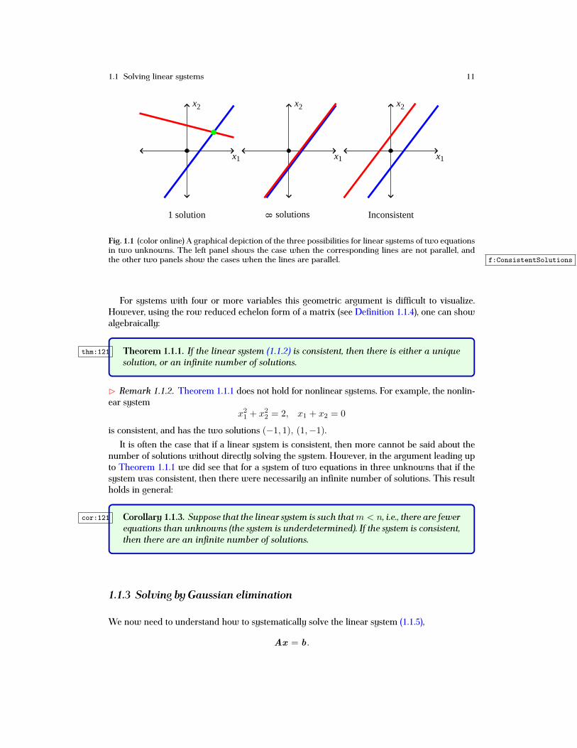
is inconsistent, as the second equation is no longer a scalar multiple of the first equation. SeeFigure 1.1 for graphical representations of these three cases.
We see that a linear system with two equations and two unknowns is either consistent withone or an infinite number of solutions, or is inconsistent. It is not difficult to show that this factholds for linear systems with three unknowns. Each linear equation in the system represents aplane in x1x2x3-space. Given any two planes, we know that they are either parallel, or intersectalong a line. Thus, if the system has two equations, then it will either be consistent with aninfinite number of solutions, or inconsistent. Suppose that the system with two equations isconsistent, and add a third linear equation. Further suppose that the original two planes intersectalong a line. This new plane is either parallel to the line, or intersects it at precisely one point. Ifthe original two planes are the same, then the new plane is either parallel to both, or intersectsit along a line. In conclusion, for a system of equations with three variables there is either aunique solution, an infinite number of solutions, or no solution.
1.1 Solving linear systems 11
x1
x2
x1
x2
x1
x2
Inconsistent1 solution solutions8
Fig. 1.1 (color online) A graphical depiction of the three possibilities for linear systems of two equationsin two unknowns. The left panel shows the case when the corresponding lines are not parallel, andthe other two panels show the cases when the lines are parallel. f:ConsistentSolutions
For systems with four or more variables this geometric argument is difficult to visualize.However, using the row reduced echelon form of a matrix (see Definition 1.1.4), one can showalgebraically:
thm:121 Theorem 1.1.1. If the linear system (1.1.2) is consistent, then there is either a uniquesolution, or an infinite number of solutions.
B Remark 1.1.2. Theorem 1.1.1 does not hold for nonlinear systems. For example, the nonlin-ear system
x21 + x22 = 2, x1 + x2 = 0
is consistent, and has the two solutions (−1, 1), (1,−1).It is often the case that if a linear system is consistent, then more cannot be said about the
number of solutions without directly solving the system. However, in the argument leading upto Theorem 1.1.1 we did see that for a system of two equations in three unknowns that if thesystem was consistent, then there were necessarily an infinite number of solutions. This resultholds in general:
cor:121 Corollary 1.1.3. Suppose that the linear system is such thatm < n, i.e., there are fewerequations than unknowns (the system is underdetermined). If the system is consistent,then there are an infinite number of solutions.
1.1.3 Solving by Gaussian elimination
We now need to understand how to systematically solve the linear system (1.1.5),
Ax = b.
12 1 Essentials of Linear Algebra
While the method of substitution works fine for two equations in two unknowns, it quicklybreaks down as a practical method when there are three or more variables involved in thesystem. We need to come up with something else.
The simplest linear system to solve for two equations in two unknowns is
x1 = b1, x2 = b2.
The coefficient matrix isI 2 =
(1 00 1
)∈M2(R),
which is known as the identity matrix. The unique solution to this system is x = b . Thesimplest linear system to solve for three equations in three unknowns is
x1 = b1, x2 = b2, x3 = b3.
The coefficient matrix is now
I 3 =
1 0 00 1 00 0 1
∈M3(R),
which is the 3 × 3 identity matrix. The unique solution to again system is x = b . Continuingin this fashion, the simplest linear system for n equations in n unknowns to solve is
x1 = b1, x2 = b2, x3 = b3, . . . , xn = bn.
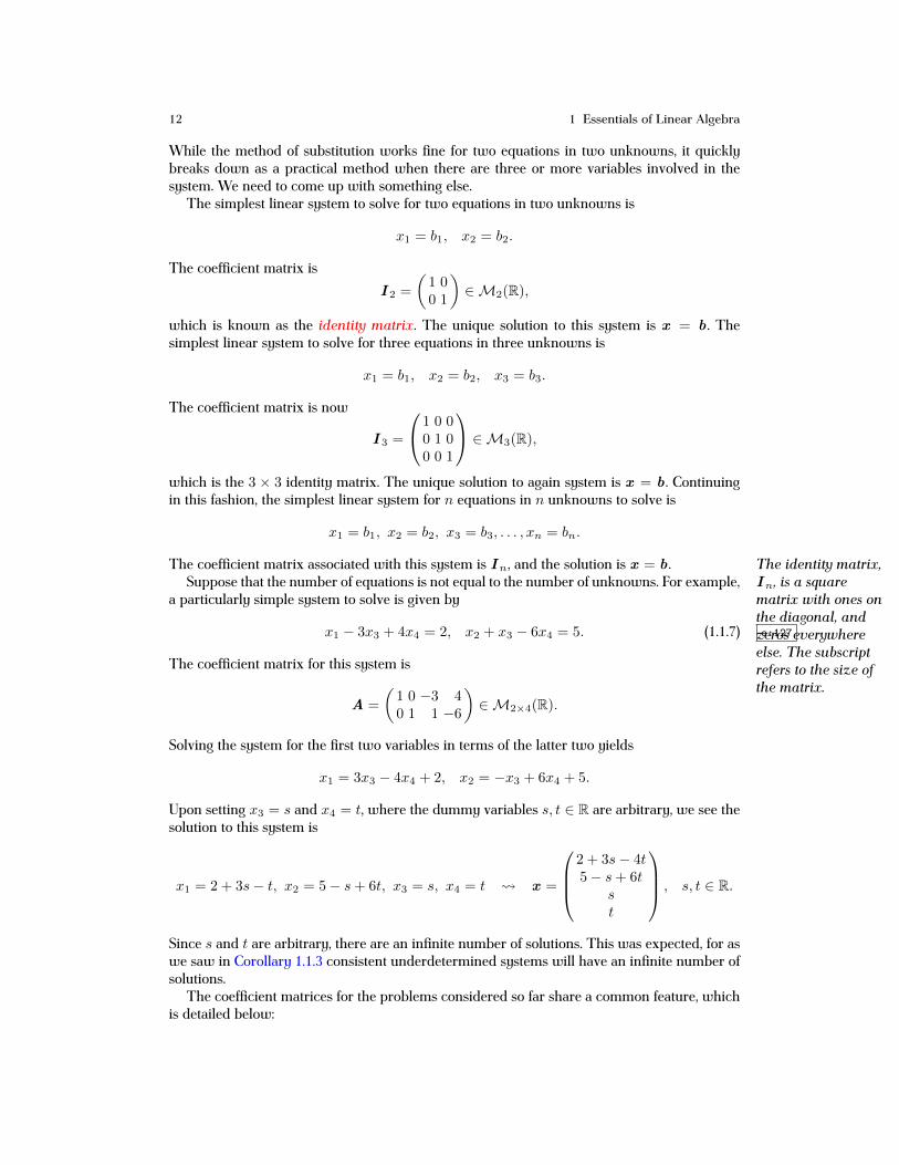
The coefficient matrix associated with this system is I n, and the solution is x = b . The identity matrix,I n, is a squarematrix with ones onthe diagonal, andzeros everywhereelse. The subscriptrefers to the size ofthe matrix.
Suppose that the number of equations is not equal to the number of unknowns. For example,a particularly simple system to solve is given by
x1 − 3x3 + 4x4 = 2, x2 + x3 − 6x4 = 5. (1.1.7) e:127
The coefficient matrix for this system is
A =
(1 0 −3 40 1 1 −6
)∈M2×4(R).
Solving the system for the first two variables in terms of the latter two yields
x1 = 3x3 − 4x4 + 2, x2 = −x3 + 6x4 + 5.
Upon setting x3 = s and x4 = t, where the dummy variables s, t ∈ R are arbitrary, we see thesolution to this system is
x1 = 2 + 3s− t, x2 = 5− s+ 6t, x3 = s, x4 = t x =
2 + 3s− 4t5− s+ 6t
st
, s, t ∈ R.
Since s and t are arbitrary, there are an infinite number of solutions. This was expected, for aswe saw in Corollary 1.1.3 consistent underdetermined systems will have an infinite number ofsolutions.
The coefficient matrices for the problems considered so far share a common feature, whichis detailed below:

1.1 Solving linear systems 13
RREFdef:121 Definition 1.1.4. A matrix is said to be in row reduced echelon form (RREF) if
(a) all nonzero rows are above any zero row(b) the first nonzero entry in a row (the leading entry) is a one(c) every other entry in a column with a leading one is zero.
Those columns with a leading entry are known as pivot columns, and the leading entriesare called pivot positions.
The RREF of a givenmatrix is unique [42].
C Example 1.1.5. Consider the matrix in RREF given by
A =
1 0 −3 0 70 1 −3 0 20 0 0 1 −40 0 0 0 0
∈M4×5(R)
The first, second, and fourth columns are the pivot columns, and the pivot positions are the firstentry in the first row, the second entry in the second row, and the fourth entry in the third row.As a rule-of-thumb,
when putting anaugmented matrix
into RREF, the idea isto place 1’s on thediagonal, and 0’s
everywhere else (asmuch as possible).
If a coefficient matrix is in RREF, then the linear system is particulary easy to solve. Thus,our goal is to take a given linear system with its attendant coefficient matrix, and then performallowable algebraic operations so that the new system has a coefficient matrix which is in RREF.The allowable algebraic operations for solving a linear system are:
(a) multiply any equation by a constant(b) add/subtract equations(c) switch the ordering of equations.
Upon doing these operations the resulting system is not the same as the original; however, thenew system is equivalent to the old in that for consistent systems the solution values remainunchanged. If the original system is inconsistent, then so will any new system resulting fromperforming the above operations.
In order to do these operations most efficiently using matrices, it is best to work with theaugmented matrix associated with the linear system Ax = b ; namely, the matrix (A|b). Theaugmented matrix is formed by adding a column, namely the vector b , to the coefficient matrix.For example, for the linear system associated with (1.1.6) the augmented matrix is given by
(A|b) =
1 0 −1 03 1 0 11 −1 −1 −4
, (1.1.8) e:128
and the augmented matrix for the linear system (1.1.7) is
(A|b) =(1 0 −3 4 20 1 1 −6 5
)The allowable operations on the individual equations in the linear system correspond to oper-ations on the rows of the augmented matrix. In particular, when doing Gaussian eliminationon an augmented matrix in order to put it into RREF, we are allowed to:
(a) multiply any row by a constant

14 1 Essentials of Linear Algebra
(b) add/subtract rows(c) switch the ordering of the rows.
Once we have performed Gaussian elimination on an augmented matrix in order to put it intoRREF, we can easily solve the resultant system.C Example 1.1.6. Consider the linear system associated with the augmented matrix in (1.1.8).We will henceforth let ρj denote the jth row of a matrix. The operation “aρj + bρk” will betaken to mean multiply the jth row by a, multiply the kth row by b, add the two resultantrows together, and replace the kth row with this sum. With this notation in mind, performingGaussian elimination yields
(A|b) −3ρ1+ρ2−→
1 0 −1 00 1 3 11 −1 −1 −4
−ρ1+ρ3−→
1 0 −1 00 1 3 10 −1 0 −4
ρ2+ρ3−→
1 0 −1 00 1 3 10 0 3 −3
(1/3)ρ3−→
1 0 −1 00 1 3 10 0 1 −1
−3ρ3+ρ2−→
1 0 −1 00 1 0 40 0 1 −1
ρ3+ρ1−→
1 0 0 −10 1 0 40 0 1 −1
.
The new linear system is
x1 = −1, x2 = 4, x3 = −1 x =
−14−1
,
which is also immediately seen to be the solution.C Example 1.1.7. Consider the linear system
x1 − 2x2 − x3 = 0
3x1 + x2 + 4x3 = 7
2x1 + 3x2 + 5x3 = 7.
Performing Gaussian elimination on the augmented matrix yields 1 −2 −1 03 1 4 72 3 5 7
−3ρ1+ρ2−→
1 −2 −1 00 7 7 72 3 5 7
−2ρ1+ρ3−→
1 −2 −1 00 7 7 70 7 7 7
−ρ2+ρ3−→
1 −2 −1 00 7 7 70 0 0 0
(1/7)ρ2−→
1 −2 −1 00 1 1 10 0 0 0
2ρ2+ρ1−→
1 0 1 20 1 1 10 0 0 0
.
The new linear system to be solved is given by
x1 + x3 = 2, x2 + x3 = 1, 0x1 + 0x2 + 0x3 = 0.
Ignoring the last equation, this is a system of two equations with three unknowns; consequently,since the system is consistent it must be the case that there are an infinite number of solutions.The variables x1 and x2 are associated with leading entries in the RREF form of the augmentedmatrix. As for the variable x3, which is associated with the third column, which in turn is nota pivot column, we say:

1.1 Solving linear systems 15
Free variabledef:121a Definition 1.1.8. A free variable of a linear system is a variable which is associated
with a column in the RREF matrix which is not a pivot column.
Since x3 is a free variable, it can be arbitrarily chosen. Upon setting x3 = t, where t ∈ R,the other variables are
x1 = 2− t, x2 = 1− t.
The solution is then
x =
2− t1− tt
, t ∈ R.
C Example 1.1.9. Consider a linear system which is a variant of the one given above; namely,
x1 − 2x2 − x3 = 0
3x1 + x2 + 4x3 = 7
2x1 + 3x2 + 5x3 = 8.
Upon doing Gaussian elimination of the augmented matrix we see that 1 −2 −1 03 1 4 72 3 5 8
RREF−→
1 0 1 20 1 1 10 0 0 1
.
The new linear system to be solved is
x1 + x3 = 2, x2 + x3 = 1, 0x1 + 0x2 + 0x3 = 1.
Since the last equation clearly does not have a solution, the system is inconsistent.C Example 1.1.10. Consider a linear system for which the coefficient matrix and nonhomoge-neous term are
A =
1 2 34 5 67 8 2
, b =
−14−7
.
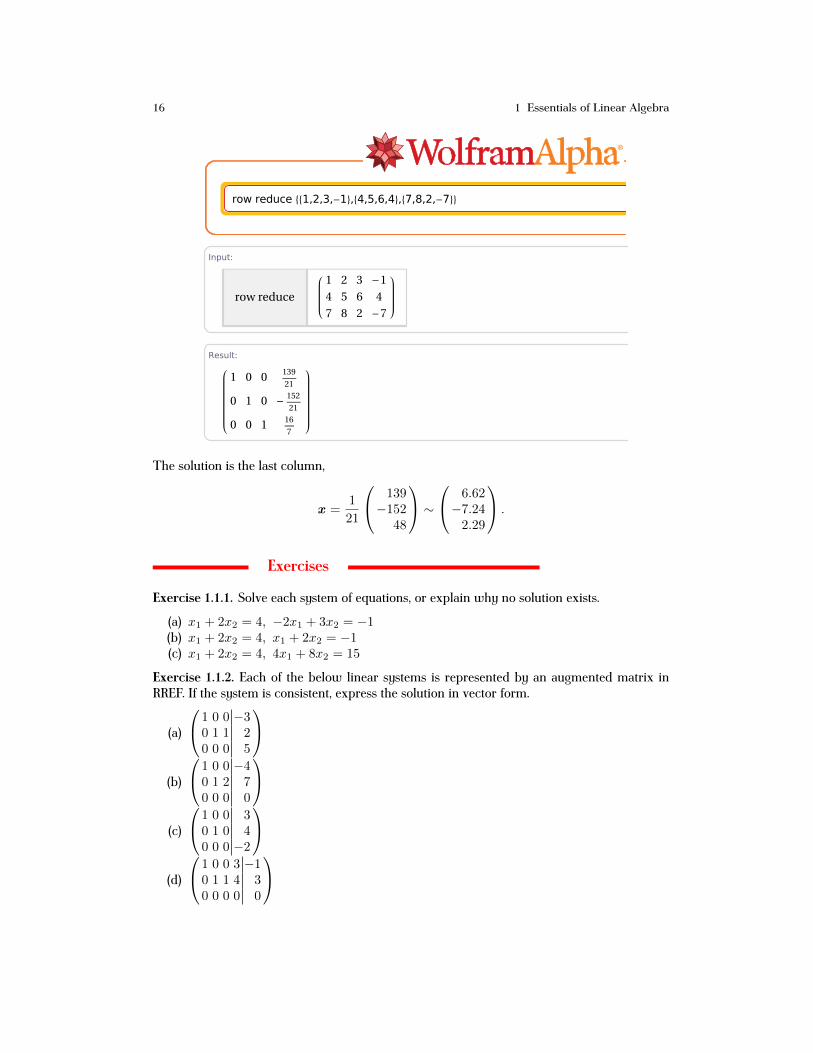
We will use WolframAlpha to put the augmented matrix into RREF. It is straightforward toenter a matrix in this CAS. The full matrix is surrounded by curly brackets. Each individualrow is also surrounded by curly brackets, and the individual entries in a row are separated bycommas. Each row is also separated by a comma. We have:
16 1 Essentials of Linear Algebra
row reduce 881,2,3,-1<,84,5,6,4<,87,8,2,-7<<
Input:
row reduce
1 2 3 -1
4 5 6 4
7 8 2 -7
Result: Step-by-step solution
1 0 0139
21
0 1 0 -152
21
0 0 116
7
Dimensions:
3 HrowsL ´ 4 HcolumnsL
Matrix plot:
1 2 3 4
1
2
3
1 2 3 4
1
2
3
Pseudoinverse: Exact form
0.57226 0.467744 -0.147709
0.467744 0.48851 0.161523
-0.147709 0.161523 0.948993
0.0646225 -0.0706664 0.0223157
Generated by Wolfram|Alpha (www.wolframalpha.com) on March 27, 2014 from Champaign, IL.
© Wolfram Alpha LLC— A Wolfram Research Company1
The solution is the last column,
x =1
21
139−152
48
∼ 6.62−7.242.29
.
Exercises
Exercise 1.1.1. Solve each system of equations, or explain why no solution exists.
(a) x1 + 2x2 = 4, −2x1 + 3x2 = −1(b) x1 + 2x2 = 4, x1 + 2x2 = −1(c) x1 + 2x2 = 4, 4x1 + 8x2 = 15
Exercise 1.1.2. Each of the below linear systems is represented by an augmented matrix inRREF. If the system is consistent, express the solution in vector form.
(a)
1 0 0 −30 1 1 20 0 0 5
(b)
1 0 0 −40 1 2 70 0 0 0
(c)
1 0 0 30 1 0 40 0 0 −2
(d)
1 0 0 3 −10 1 1 4 30 0 0 0 0

1.1 Solving linear systems 17
Exercise 1.1.3. Determine all value(s) of r which make each augmented matrix correspond toa consistent linear system. For each such r, express the solution to the corresponding linearsystem in vector form.
(a)(
1 4 −3−2 −8 r
)(b)(1 4 −32 r −6
)(c)(
1 4 −3−3 r −9
)(d)(
1 r −3−3 r 8
)Exercise 1.1.4. The augmented matrix for a linear system is given by1 1 3 2
1 2 4 31 3 a b
.
(a) For what value(s) of a and b will the system have infinitely many solutions?(b) For what value(s) of a and b will the system be inconsistent?
Exercise 1.1.5. Solve each linear system, and express the solution in vector form.
(a) 3x1 + 2x2 = 16, −2x1 + 3x2 = 11(b) 3x1 + 2x2 − x3 = −2, −3x1 − x2 + x3 = 5, 3x1 + 2x2 + x3 = 2(c) 2x1 + x2 = −1, x1 − x3 = −2, −x1 + 3x2 + 7x3 = 11(d) x1 + x2 − x3 = 0, 2x1 − 3x2 + 5x3 = 0, 4x1 − x2 + 3x3 = 0(e) x2 + x3 − x4 = 0, x1 + x2 + x3 + x4 = 6
2x1 + 4x2 + x3 − 2x4 = −1, 3x1 + x2 − 2x3 + 2x4 = 3
Exercise 1.1.6. If the coefficient matrix satisfies A ∈ M9×6(R), and if the RREF of the aug-mented matrix (A|b) has three zero rows, is the solution unique? Why, or why not?Exercise 1.1.7. If the coefficient matrix satisfies A ∈M5×7(R), and if the linear system Ax =b is consistent, is the solution unique? Why, or why not?Exercise 1.1.8. Determine if each of the following statements is true or false. Provide an expla-nation for your answer.
(a) A system of four linear equations in three unknowns can have exactly five solutions.(b) If a system has a free variable, then there will be an infinite number of solutions.(c) If a system is consistent, then there is a free variable.(d) If the RREF of the augmented matrix has four zero rows, and if the system is consistent,
then there will be an infinite number of solutions.(e) If the RREF of the augmented matrix has no zero rows, then the system is consistent.
Exercise 1.1.9. Find a quadratic polynomial p(t) = a0 + a1t+ a2t2 which passes through the
points (−2, 12), (1, 6), (2, 18). Hint: p(1) = 6 implies that a0 + a1 + a2 = 6.Exercise 1.1.10. Find a cubic polynomial p(t) = a0 + a1t+ a2t
2 + a3t3 which passes through
the points (−1,−3), (0, 1), (1, 3), (2, 17).

18 1 Essentials of Linear Algebra
1.2 Vector algebra and matrix/vector multiplication
Now that we have an efficient algorithm to solve the linear system Ax = b , we need to nextunderstand what it means from a geometric perspective to solve the system. For example, if thesystem is consistent, how does the vector b relate to the coefficients of the coefficient matrix A?In order to answer this question, we need to make sense of the expression Ax (matrix/vectormultiplication).
1.2.1 Linear combinations of vectors
We begin by considering the addition/subtraction of vectors, and the product of a scalar with avector. We will define the addition/subtraction of two n-vectors to be exactly what is expected,and the same will hold true for the multiplication of a vector by a scalar; namely,
x ± y =
x1 ± y1x2 ± y2
...xn ± yn
, cx =
cx1cx2
...cxn
.
Vector addition and subtraction are done component-by-component, and scalar multiplicationof a vector means that each component of the vector is multiplied by the scalar. For example,(
−25
)+
(3−1
)=
(14
), 3
(2−3
)=
(6−9
).
These are linear operations. Combining these two operations, we have more generally:
Linear combinationdef:131 Definition 1.2.1. A linear combination of the n-vectors a1, . . . ,ak is given by the vec-
tor b , where
b = x1a1 + x2a2 + · · ·+ xkak =
k∑j=1
xjaj .
The scalars x1, . . . , xk are known as weights.
With this notion of linear combinations of vectors, we can rewrite linear systems of equationsin vector notation. For example, consider the linear system
x1 − x2 + x3 = −13x1 + 2x2 + 8x3 = 7
x1 + 2x2 + 4x3 = 5.
(1.2.1) e:131
Since two vectors are equal if and only if all of their coefficients are equal, we can write (1.2.1)in vector form as x1 − x2 + x3
3x1 + 2x2 + 8x3x1 + 2x2 + 4x3
=
−175
.

1.2 Vector algebra and matrix/vector multiplication 19
Using linearity we can write the vector on the left-hand side as x1 − x2 + x33x1 + 2x2 + 8x3x1 + 2x2 + 4x3
= x1
131
+ x2
−122
+ x3
184
,
so the system (1.2.1) is equivalent to
x1
131
+ x2
−122
+ x3
184
=
−175
.
After setting
a1 =
131
, a2 =
−122
, a3 =
184
, b =
−175
,
the linear system can then be rewritten as the linear combination of vectors
x1a1 + x2a2 + x3a3 = b. (1.2.2) e:132
In conclusion, asking for solutions to the linear system (1.2.1) can instead be thought of asasking if the vector b is a linear combination of the vectors a1,a2,a3. It can be checked thatafter Gaussian elimination 1 −1 1 −1
3 2 8 71 2 4 5
RREF−→
1 0 2 10 1 1 20 0 0 0
.
The free variable is x3, so the solution to the linear system (1.2.1) can be written
x1 = 1− 2t, x2 = 2− t, x3 = t; t ∈ R. (1.2.3) e:132a
In vector form this form of the solution is
x =
1− 2t2− tt
=
120
+ t
−2−11
, t ∈ R.
The vector b is a linear combination of the vectors a1,a2,a3, and the weights are given in(1.2.3),
b = (1− 2t)a1 + (2− t)a2 + ta3, t ∈ R.
1.2.2 Matrix/vector multiplication
With this observation in mind, we now define the multiplication of a matrix and a vector sothat the resultant corresponds to a linear system. For the linear system of (1.2.1) let A be thecoefficient matrix,
A = (a1 a2 a3) ∈M3(R).

20 1 Essentials of Linear Algebra
Here each column of A is thought of as a vector. If for
x =
x1x2x3
we define
Ax := x1a1 + x2a2 + x3a3,
then by using (1.2.2) we have that the linear system is given by
Ax = b (1.2.4) e:133
(compare with (1.1.5)). In other words, by writing the linear system in the form of (1.2.4) wereally mean the linear combinations of (1.2.2), which in turn is equivalent to the original system(1.2.1).
Matrix/vector multiplication
def:132 Definition 1.2.2. Suppose that A = (a1 a2 · · · an), where each vector aj ∈ Rm isan m-vector. For x ∈ Rn we define matrix/vector multiplication as
Ax = x1a1 + x2a2 + · · ·+ xnan =
n∑j=1
xjaj .
Note that A ∈Mm×n(R) and x ∈ Rn, so by definition
A︸︷︷︸Rm×n
x︸︷︷︸Rn×1
= b︸︷︷︸Rm×1
.
In order for a matrix/vector multiplication to make sense, the number of columns in the matrixA must the be same as the number of entries in the vector x . The product will be a vector inwhich the number of entries is equal to the number of rows in A.C Example 1.2.3. We have(
1 23 4
)(−35
)= −3
(13
)+ 5
(24
)=
(711
),
and (1 2 53 4 6
) 2−13
= 2
(13
)−(24
)+ 3
(56
)=
(1520
).
Note that in the first example a 2 × 2 matrix multiplied a 2 × 1 matrix in order to get a 2 × 1matrix, whereas in the second example a 2× 3 matrix multiplied a 3× 1 matrix in order to geta 2× 1 matrix.
The multiplication of a matrix and a vector is a linear operation, as it satisfies the propertythat the product of a matrix with a linear combination of vectors is the same thing as first takingthe individual matrix/vector products, and then taking the appropriate linear combination ofthe resultant two vectors:
1.2 Vector algebra and matrix/vector multiplication 21
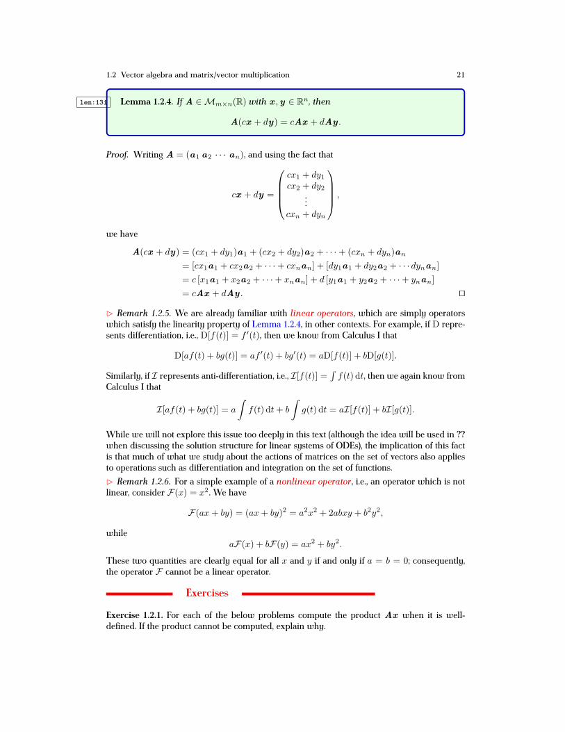
lem:131 Lemma 1.2.4. If A ∈Mm×n(R) with x ,y ∈ Rn, then
A(cx + dy) = cAx + dAy .
Proof. Writing A = (a1 a2 · · · an), and using the fact that
cx + dy =
cx1 + dy1cx2 + dy2
...cxn + dyn
,
we have
A(cx + dy) = (cx1 + dy1)a1 + (cx2 + dy2)a2 + · · ·+ (cxn + dyn)an
= [cx1a1 + cx2a2 + · · ·+ cxnan] + [dy1a1 + dy2a2 + · · · dynan]= c [x1a1 + x2a2 + · · ·+ xnan] + d [y1a1 + y2a2 + · · ·+ ynan]
= cAx + dAy . ut
B Remark 1.2.5. We are already familiar with linear operators, which are simply operatorswhich satisfy the linearity property of Lemma 1.2.4, in other contexts. For example, if D repre-sents differentiation, i.e., D[f(t)] = f ′(t), then we know from Calculus I that
D[af(t) + bg(t)] = af ′(t) + bg′(t) = aD[f(t)] + bD[g(t)].
Similarly, if I represents anti-differentiation, i.e., I[f(t)] =∫f(t) dt, then we again know from
Calculus I that
I[af(t) + bg(t)] = a
∫f(t) dt+ b
∫g(t) dt = aI[f(t)] + bI[g(t)].
While we will not explore this issue too deeply in this text (although the idea will be used in ??when discussing the solution structure for linear systems of ODEs), the implication of this factis that much of what we study about the actions of matrices on the set of vectors also appliesto operations such as differentiation and integration on the set of functions.B Remark 1.2.6. For a simple example of a nonlinear operator, i.e., an operator which is notlinear, consider F(x) = x2. We have
F(ax+ by) = (ax+ by)2 = a2x2 + 2abxy + b2y2,
whileaF(x) + bF(y) = ax2 + by2.
These two quantities are clearly equal for all x and y if and only if a = b = 0; consequently,the operator F cannot be a linear operator.
Exercises
Exercise 1.2.1. For each of the below problems compute the product Ax when it is well-defined. If the product cannot be computed, explain why.
22 1 Essentials of Linear Algebra
(a) A =
(1 −3−3 2
), x =
(−42
)(b) A =
(1 −2 52 0 −3
), x =
2−17
(c) A =
1 −25 20 −3
, x =
2−17
(d) A =
(2 −1 −3
), x =
16−4
.
Exercise 1.2.2. Let
a1 =
−121
, a2 =
311
, a3 =
153
, b =
−315
.
Is b a linear combination of a1,a2,a3? If so, are the weights unique?Exercise 1.2.3. Let
A =
(2 5−3 −1
), b =
(56
).
Is the linear system Ax = b consistent? If so, what particular linear combination(s) of thecolumns of A give the vector b?Exercise 1.2.4. Find all of the solutions to the homogeneous problem Ax = 0 when:
(a) A =
(1 −3 62 0 7
)(b) A =
1 −3 −4−2 4 −120 2 −4
(c) A =
2 3 6−3 5 −11 −1 1
Exercise 1.2.5. Let
A =
(2 −1−6 3
), b =
(b1b2
).
Describe the set of all vectors b for which Ax = b is consistent.Exercise 1.2.6. Determine if each of the following statements is true or false. Provide an expla-nation for your answer.
(a) The homogeneous system Ax = 0 is consistent.(b) If b is a linear combination of a1,a2, then there exist unique scalars x1, x2 such that
b = x1a1 + x2a2.(c) If Ax = b is consistent, then b is a linear combination of the rows of A.(d) A linear combination of five vectors in R3 produces a vector in R5.(e) In order to compute Ax , the vector x must have the same number of entries as the
number of rows in A.
1.3 Matrix algebra: addition, subtraction, and multiplication 23
1.3 Matrix algebra: addition, subtraction, and multiplications:18
Now that we have defined vector algebra and matrix/vector multiplication, we briefly considerthe algebra of matrices; in particular, addition, subtraction, and multiplication. Division will bediscussed later in Chapter 1.11. Just like for vectors, the addition and subtraction are straight-forward, as is scalar multiplication. If we denote two matrices as A = (ajk) ∈Mm×n(R) andB = (bjk) ∈Mm×n(R), then it is the case that
A±B = (ajk ± bjk), cA = (cajk).
In other words, we add/subtract two matrices of the same size component-by-component, andif we multiply a matrix by a scalar, then we multiply each component by that scalar. This isexactly what we do in the addition/subtraction of vectors, and the multiplication of a vector bya scalar. For example, if
A =
(1 2−1 −3
), B =
(2 14 3
),
thenA+B =
(3 33 0
), 3A =
(3 6−3 −9
).
Regarding the multiplication of two matrices, we simply generalize the matrix/vector multi-plication. For a given A ∈Mm×n(R), recall that for b ∈ Rn,
Ab = b1a1 + b2a2 + · · ·+ bnan, A = (a1 a2 · · · an).
If B = (b1 b2 · · · b`) ∈ Mn×`(R) (note that each column bj ∈ Rn), we then define themultiplication of A and B by
A︸︷︷︸Mm×n(R)
B︸︷︷︸Mn×`(R)
= (Ab1 Ab2 · · · Ab`)︸ ︷︷ ︸Mm×`(R)
.
The number of columns of A must match the number of rows of B in order for the operationto make sense. Furthermore, the number of rows of the product is the number of rows of A,and the number of columns of the product is the number of columns of B . For example, if
A =
(1 2 3−1 −3 2
), B =
2 14 36 4
,
then
AB =
A
246
A
134
=
(28 19−2 −2
)∈M2(R),
and
BA =
(B
(1−1
)B
(2−3
)B
(32
))=
1 1 81 −1 182 0 26
∈M3(R).
As the above example illustrates, it may not necessarily be the case that AB = BA. In thisexample changing the order of multiplication leads to a resultant matrices of different sizes.However, even if the resultant matrices are the same size, they need not be the same. Suppose
24 1 Essentials of Linear Algebra
thatA =
(1 2−1 −3
), B =
(2 14 3
).
We haveAB =
(A
(24
)A
(13
))=
(10 7−14 −10
)∈M2(R),
andBA =
(B
(1−1
)B
(2−3
))=
(1 11 −1
)∈M2(R).
These are clearly not the same matrix. Thus, in general we cannot expect matrix multiplicationto be commutative.
On the other hand, even though matrix multiplication is not necessarily commutative, it isassociative, i.e.,
A(B +C ) = AB +AC .
This fact follows from the fact that matrix/vector multiplication is a linear operation (recallLemma 1.2.4), and the definition of matrix/matrix multiplication through matrix/vector multi-plication. In particular, if we write
B = (b1 b2 · · · b`), C = (c1 c2 · · · c`),
then upon writingB +C = (b1 + c1 b2 + c2 · · · b` + c`)
we have
A(B +C ) = A(b1 + c1 b2 + c2 · · · b` + c`)
= (A(b1 + c1) A(b2 + c2) · · · A(b` + c`))
= (Ab1 +Ac1 Ab2 +Ac2 · · · Ab` +Ac`)
= (Ab1 Ab2 · · · Ab`) + (Ac1 Ac2 · · · Ac`)
= AB +AC .
Indeed, while we will not discuss the details here, it is a fact that just like matrix/vector multi-plication, matrix/matrix multiplication is a linear operation,
A(bB + cC ) = bAB + cAC .
There is a special matrix which plays the role of the scalar 1 in matrix multiplication: theidentity matrix I n. If A ∈Mm×n(R), then it is straightforward to check that
AI n = A, ImA = A.
In particular, if x ∈ Rn, then it is true that I nx = x . For an explicit example of this fact, ifn = 3, 1 0 0
0 1 00 0 1
x1x2x3
= x1
100
+ x2
010
+ x3
001
=
x1x2x3
.
Exercises

1.4 Sets of linear combinations of vectors 25
Exercise 1.3.1. Let
A =
(1 −2 −5−2 3 −7
), B =
2 0−2 31 5
, C =
1 25 −43 −1
.
Compute the prescribed algebraic operation if it is well-defined. If it cannot be done, explainwhy.
(a) 3B − 2C(b) 4A+ 2B(c) AB(d) CA
Exercise 1.3.2. Suppose that A ∈Mm×n(R) and B ∈Mn×k(R) with m 6= n and n 6= k (i.e.,neither matrix is square).
(a) What is the size of AB?(b) Can m, k be chosen so that BA is well-defined? If so, what is the size of BA?(c) Is is possible for AB = BA? Explain.
1.4 Sets of linear combinations of vectorss:13
Consider the linear system,
Ax = b, A = (a1 a2 · · · ak) ,
which by the definition of matrix/vector multiplication can be written,
x1a1 + x2a2 + · · ·+ xkak = b.
The linear system is consistent if and only if the vector b is some linear combination of thevectors a1,a2, . . . ,ak . We now study the set of all linear combinations of these vectors. Oncethis set has been properly described, we will consider the problem of determining which (andhow many) of the original set of vectors are needed in order to adequately describe it.
1.4.1 Span of a set of vectors
A particular linear combination of the vectors a1,a2, . . . ,ak is given by x1a1 + · · · + xkak .The collection of all possible linear combinations of these vectors is known as the span of thevectors.

26 1 Essentials of Linear Algebra
Span
def:141 Definition 1.4.1. Let S = {a1,a2, . . . ,ak} be a set of n-vectors. The span of S,
Span(S) = Span {a1,a2, . . . ,ak} ,
is the collection of all linear combinations. In other words, b ∈ Span(S) if and only iffor some x ∈ Rk ,
b = x1a1 + x2a2 + · · ·+ xkak.
The span of a collection of vectors has geometric meaning. First suppose that a1 ∈ R3. Recallthat lines in R3 are defined parametrically by
r(t) = r0 + tv ,
where v is a vector parallel to the line and r0 corresponds to a point on the line. Since
Span {a1} = {ta1 : t ∈ R} ,
this set is the line through the origin which is parallel to a1.Now suppose that a1,a2 ∈ R3 are not parallel, i.e., a2 6= ca1 for some c ∈ R. Set v =
a1 × a2, i.e., v is a 3-vector which is perpendicular to both a1 and a2. The linearity of the dotproduct, and the fact that v · a1 = v · a2 = 0, yields
v · (x1a1 + x2a2) = x1v · a1 + x2v · a2 = 0.
Thus,Span {a1,a2} = {x1a1 + x2a2 : x1, x2 ∈ R}
is the collection of all vectors which are perpendicular to v . In other words, Span {a1,a2} is theplane through the origin which is perpendicular to v . There are higher dimensional analogues,but unfortunately they are difficult to visualize.
Now let us consider the computation that must be done in order to determine if b ∈ Span(S).By definition b ∈ Span(S), i.e., b is a linear combination of the vectors a1, . . . ,ak , if and onlyif there exist constants x1, x2, . . . , xk such that
x1a1 + x2a2 + · · ·+ xkak = b.
Upon setting
A = (a1 a2 · · · ak), x =
x1x2...xk
,
by using the Definition 1.2.2 of matrix/vector multiplication we have that this condition is equiv-alent to solving the linear system Ax = b . This yields:
rem:141 Lemma 1.4.2. Suppose that S = {a1,a2, . . . ,ak}, and set A = (a1 a2 · · · ak). Thevector b ∈ Span(S) if and only if the linear system Ax = b is consistent.
C Example 1.4.3. Letting

1.4 Sets of linear combinations of vectors 27
a1 =
(12
), a2 =
(11
), b =
(−12
),
let us determine if b ∈ Span {a1,a2}. As we have seen in Lemma 1.4.2, this question is equiva-lent to determining if the linear system Ax = b is consistent. Since after Gaussian elimination
(A|b) RREF−→(1 0 30 1 −4
),
the linear system Ax = b is equivalent to
x1 = 3, x2 = −4,
which is easily solved. Thus, not only is b ∈ Span {a1,a2}, but it is the case that b = 3a1−4a2.C Example 1.4.4. Letting
a1 =
12−4
, a2 =
3−15
, b =
7−7r
,
let us determine those value(s) of r for which b ∈ Span {a1,a2}. As we have seen inLemma 1.4.2, this question is equivalent to determining if the linear system Ax = b is consis-tent. Since after Gaussian elimination
(A|b) RREF−→
1 0 −20 1 30 0 r − 23
,
the linear system is consistent if and only if r = 23. In this case x1 = −2, x2 = 3, so thatb ∈ Span {a1,a2} with b = −2a1 + 3a2.
Spanning set
def:spanset Definition 1.4.5. Let S = {a1,a2, . . . ,ak}, where each vector aj ∈ Rn. We say thatS is a spanning set for Rn if each b ∈ Rn is realized as a linear combination of thevectors in S,
b = x1a1 + x2a2 + · · ·+ xkak.
In other words, S is a spanning set if the linear system,
Ax = b, A = (a1 a2 · · · ak) ,
is consistent for any b .
C Example 1.4.6. For
a1 =
121
, a2 =
3−42
, a3 =
4−23
, a4 =
47−5
,
let us determine if S = {a1,a2,a3,a4} is a spanning set for R3. Using Lemma 1.5.2 we needto know if Ax = b is consistent for any b ∈ R3, where A = (a1 a2 a3 a4). In order for this

28 1 Essentials of Linear Algebra
to be the case, the RREF of the augmented matrix (A|b) must always correspond to a consistentsystem; in particular, the coefficient side of the RREF of the augmented matrix must have nozero rows. Thus, in order to answer the question it is sufficient to consider the RREF of A. Since
ARREF−→
1 0 1 00 1 1 00 0 0 1
,
which has no zero rows, the linear system will always be consistent. The set S is a spanningset for R3.
1.4.2 Linear independence of a set of vectors
We now consider the question of how many of the vectors a1,a2, . . . ,ak are needed to com-pletely describe Span ({a1,a2, . . . ,ak}). For example, let S = {a1,a2,a3}, where
a1 =
1−10
, a2 =
101
, a3 =
5−23
.
and consider Span(S). If b ∈ Span(S), then upon using Definition 1.4.1 we know there existconstants x1, x2, x3 such that
b = x1a1 + x2a2 + x3a3.
Now, it can be checked that
a3 = 2a1 + 3a2 a1 + 3a2 − a3 = 0 , (1.4.1) e:132aa
so the vector a3 is a linear combination of a1 and a2. The original linear combination can bethen rewritten as
b = x1a1 + x2a2 + x3(2a1 + 3a2) = (x1 + 2x3)a1 + (x2 + 3x3)a2.
In other words, the vector b is a linear combination of a1 and a2 alone. Thus, the addition ofa3 in the definition of Span(S) is superfluous, so we can write
Span(S) = Span {a1,a2} .
Since a2 6= ca1 for some c ∈ R, we cannot reduce the collection of vectors comprising thespanning set any further.
We say that if some nontrivial linear combination of some set of vectors produces the zerovector, such as in (1.4.1), then:
In the precedingexample the set{a1,a2,a3} islinearly dependent,whereas the set{a1,a2} is linearlyindependent.

1.4 Sets of linear combinations of vectors 29
Linear dependence
def:161 Definition 1.4.7. The set of vectors S = {a1,a2, . . . ,ak} is linearly dependent if thereis a nontrivial vector x 6= 0 ∈ Rk such that
x1a1 + x2a2 + · · ·+ xkak = 0 . (1.4.2) e:163
Otherwise, the set of vectors is linearly independent.
If the set of vectors is linearly dependent, then (at least) one vector in the collection can bewritten as a linear combination of the other vectors (again see (1.4.1)). In particular, two vec-tors will be linearly dependent if and only if one is a multiple of the other. An examination of(1.4.2) through the lens of matrix/vector multiplication reveals the left-hand side is Ax . Conse-quently, we determine if a set of vectors is linearly dependent or independent by solving thehomogeneous linear system
Ax = 0 , A = (a1 a2 · · · ak).
If there is a nontrivial solution, i.e., a solution other than the zero vector, then the vectors willbe linearly dependent; otherwise, they will be independent.
lem:161a Lemma 1.4.8. Let S = {a1,a2, . . . ,ak} be a set of n-vectors, and set
A = (a1 a2 · · · ak) ∈Mn×k(R).
The vectors are linearly dependent if and only the linear system Ax = 0 has anontrivial solution. Alternatively, the vectors are linearly independent if and only ifthe only solution to Ax = 0 is x = 0 .
Regarding the homogeneous problem, note that if
Ax = 0 ,
then by the linearity of matrix/vector multiplication,
0 = cAx = A (cx ) , c ∈ R.
In other words, if x is a solution to the homogeneous problem, then so is cx for any constantc. Thus, if the homogeneous system has one nontrivial solution, there will necessarily be aninfinite number of such solutions. Moreover, there can be nontrivial (nonzero) solutions to thehomogeneous problem if and only if there are free variables. In particular, if all of the columnsof A are pivot columns, then the vectors must be linearly independent.
When solving the homogeneous system by Gaussian elimination, it is enough to row reducethe matrix A only. The augmented matrix (A|0 ) yields no additional information, as the right-most column remains the zero vector no matter what algebraic operations are performed. Withthese observations in mind we can restate Lemma 1.4.8:

30 1 Essentials of Linear Algebra
cor:161aa Corollary 1.4.9. Let S = {a1,a2, . . . ,ak} be a set of n-vectors, and set
A = (a1 a2 · · · ak) ∈Mn×k(R).
The vectors are linearly independent if and only if all of the columns of A are pivotcolumns.
C Example 1.4.10. Let
a1 =
101
, a2 =
3−14
, a3 =
−11−2
, a4 =
−33−2
,
and consider the sets
S1 = {a1,a2} , S2 = {a1,a2,a3} , S3 = {a1,a2,a3,a4} .
For each set of vectors we wish to determine if they are linearly independent. If they are not,then we will write down a linear combination of the vectors that yields the zero vector.
Forming the augmented matrix and performing Gaussian elimination gives the RREF of eachgiven matrix to be
A1 = (a1 a2)RREF−→
1 00 10 0
, A2 = (a1 a2 a3)RREF−→
1 0 20 1 −10 0 0
,
and
A3 = (a1 a2 a3 a4)RREF−→
1 0 2 00 1 −1 00 0 0 1
.
By Corollary 1.4.9 the vectors in S1 are linearly independent. However, the same cannot be saidfor the latter two sets.
The homogeneous linear system associated with the RREF of A2 is
x1 + 2x3 = 0, x2 − x3 = 0.
Since x3 is a free variable, a solution is
x1 = −2t, x2 = t, x3 = t x =
−211
, t ∈ R.
Using the definition of matrix/vector multiplication we conclude the relationship,
0 = A2
−211
= −2a1 + a2 + a3.
Moreover,a3 = 2a1 − a2 Span{a1,a2,a3} = Span{a1,a2}.
The homogeneous linear system associated with the RREF of A3 is

1.4 Sets of linear combinations of vectors 31
x1 + 2x3 = 0, x2 − x3 = 0, x4 = 0.
Since x3 is still a free variable, a solution is
x1 = −2t, x2 = t, x3 = t, x4 = 0 x =
−2110
, t ∈ R.
Using the definition of matrix/vector multiplication we conclude the relationship as before,
0 = A3
−2110
= −2a1 + a2 + a3.
Moreover,
a3 = 2a1 − a2 Span{a1,a2,a3,a4} = Span{a1,a2,a4}.
C Example 1.4.11. Suppose that S = {a1,a2,a3,a4,a5}, where each aj ∈ R4. Furthersuppose that the RREF of A is
A = (a1 a2 a3 a4 a5)RREF−→
1 0 2 0 −30 1 −1 1 20 0 0 0 00 0 0 0 0
.
The first two columns of A are the pivot columns, and the remaining columns are associatedwith free variables. The homogeneous system associated with the RREF of A is
x1 + 2x3 − 3x5 = 0, x2 − x3 + x4 + 2x5 = 0.
Since x3, x4, x5 are free variables, in vector form the solution to the homogeneous system is
x = r
−21100
+ s
0−1010
+ t
3−2001
r, s, t ∈ R.
We then have the relationships,
0 = A
−21100
= −2a1 + a2 + a3,
and
32 1 Essentials of Linear Algebra
0 = A
0−1010
= −a2 + a4,
and
0 = A
3−2001
= 3a1 − 2a2 + a5.
The last three vectors are each a linear combination of the first two,
a3 = 2a1 − a2, a4 = a2, a5 = −3a1 + 2a2,
soSpan {a1,a2,a3,a4,a5} = Span {a1,a2} .
1.4.3 Linear independence of a set of functionss:wronskian
When discussing linear dependence we can use Definition 1.4.7 in a more general sense. Sup-pose that {f1, f2, . . . , fk} is a set of real-valued functions, each of which has at least k− 1 con-tinuous derivatives. We say that these functions are linearly dependent on the interval a < t < bif there is a nontrivial vector x ∈ Rk such that
x1f1(t) + x2f2(t) + · · ·+ xkfk(t) ≡ 0, a < t < b.
How do we determine if this set of functions is linearly dependent? The problem is that unlikethe previous examples it is not at all clear how to formulate this problem as a homogeneouslinear system.
We overcome this difficulty in the following manner. Suppose that the functions are linearlydependent. Since the linear combination of the functions is identically zero, it will be the casethat a derivative of the linear combination will also be identically zero, i.e.,
x1f′1(t) + x2f
′2(t) + · · ·+ xkf
′k(t) ≡ 0, a < t < b.
We can take a derivative of the above to then get
x1f′′1 (t) + x2f
′′2 (t) + · · ·+ xkf
′′k (t) ≡ 0, a < t < b,
and continuing in the fashion we have for j = 0, . . . , k − 1,
x1f(j)1 (t) + x2f
(j)2 (t) + · · ·+ xkf
(j)k (t) ≡ 0, a < t < b.
We have now derived a system of k linear equations, which is given by
1.4 Sets of linear combinations of vectors 33
W (t)x ≡ 0 , W (t) :=
f1(t) f2(t) · · · fk(t)f ′1(t) f ′2(t) · · · f ′k(t)f ′′1 (t) f ′′2 (t) · · · f ′′k (t)
......
......
f(k−1)1 (t) f
(k−1)2 (t) · · · f (k−1)k (t)
.
The matrix W (t) is known as the Wronskian for the set of functions {f1(t), f2(t), . . . , fk(t)}.We now see that the functions will be linearly dependent if there is a nontrivial vector x ,
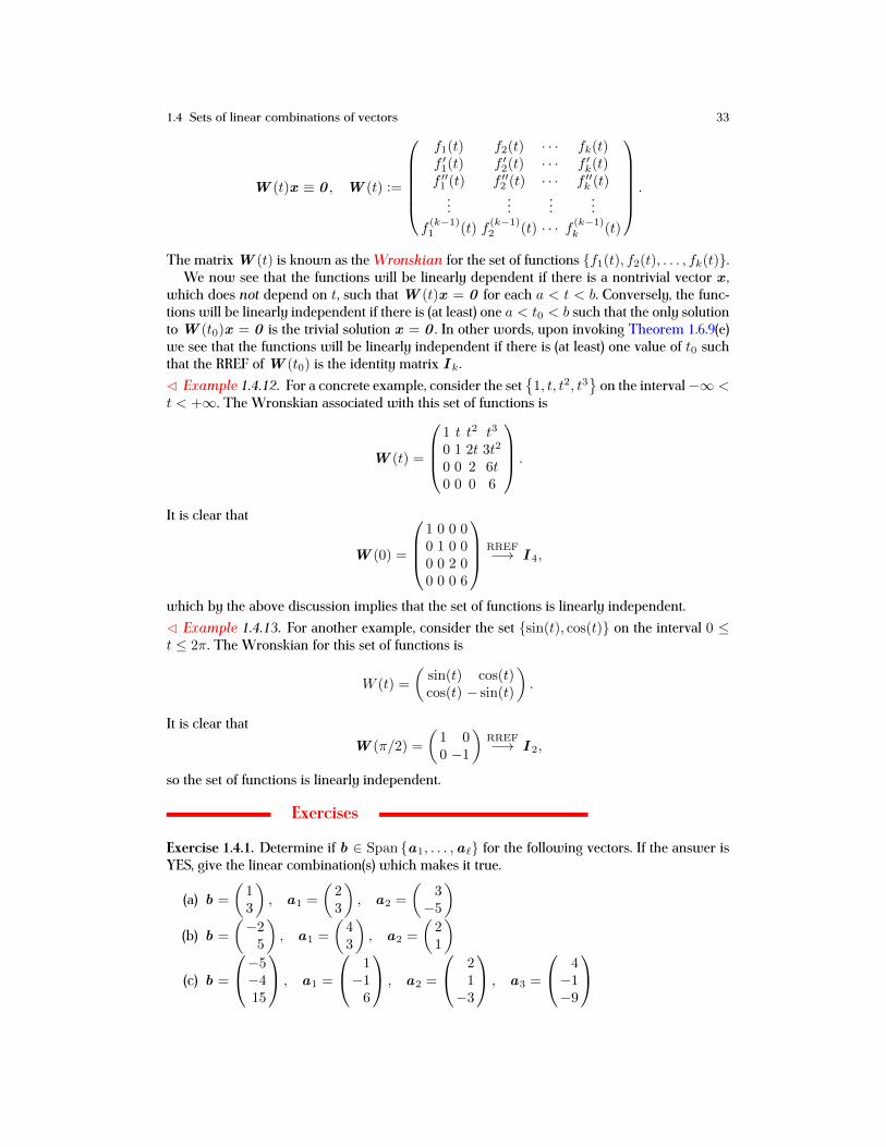
which does not depend on t, such that W (t)x = 0 for each a < t < b. Conversely, the func-tions will be linearly independent if there is (at least) one a < t0 < b such that the only solutionto W (t0)x = 0 is the trivial solution x = 0 . In other words, upon invoking Theorem 1.6.9(e)we see that the functions will be linearly independent if there is (at least) one value of t0 suchthat the RREF of W (t0) is the identity matrix I k .C Example 1.4.12. For a concrete example, consider the set
{1, t, t2, t3
}on the interval−∞ <
t < +∞. The Wronskian associated with this set of functions is
W (t) =
1 t t2 t3
0 1 2t 3t2
0 0 2 6t0 0 0 6
.
It is clear that
W (0) =
1 0 0 00 1 0 00 0 2 00 0 0 6
RREF−→ I 4,
which by the above discussion implies that the set of functions is linearly independent.C Example 1.4.13. For another example, consider the set {sin(t), cos(t)} on the interval 0 ≤t ≤ 2π. The Wronskian for this set of functions is
W (t) =
(sin(t) cos(t)cos(t) − sin(t)
).
It is clear thatW (π/2) =
(1 00 −1
)RREF−→ I 2,
so the set of functions is linearly independent.
Exercises
Exercise 1.4.1. Determine if b ∈ Span {a1, . . . ,a`} for the following vectors. If the answer isYES, give the linear combination(s) which makes it true.
(a) b =
(13
), a1 =
(23
), a2 =
(3−5
)(b) b =
(−25
), a1 =
(43
), a2 =
(21
)(c) b =
−5−415
, a1 =
1−16
, a2 =
21−3
, a3 =
4−1−9

34 1 Essentials of Linear Algebra
(d) b =
1−24
, a1 =
130
, a2 =
3−15
, a3 =
1−11
Exercise 1.4.2. Find the equation of the line in R2 which corresponds to Span {v1}, where
v1 =
(2−5
).
Exercise 1.4.3. Find the equation of the plane inR3 which corresponds to Span {v1, v2}, where
v1 =
1−2−1
, v2 =
304
.
Exercise 1.4.4. Determine if each of the following statements is true or false. Provide an expla-nation for your answer.
(a) The span of any two nonzero vectors in R3 can be viewed as a plane through the originin R3.
(b) If Ax = b is consistent, then b ∈ Span {a1,a2, . . . ,an} for A = (a1 a2 · · · an).(c) The number of free variables for a linear system is the same as the number of pivot
columns for the coefficient matrix.(d) The span of a single nonzero vector in R2 can be viewed as a line through the origin in
R2.
Exercise 1.4.5. Is the set of vectors,
S =
2−146
,
1−168
,
032−5
,
−1107
,
a spanning set for R4? Why, or why not?Exercise 1.4.6. Determine if the set of vectors is linearly independent. If the answer is NO, givethe weights for the linear combination which results in the zero vector.
(a) a1 =
(1−4
), a2 =
(−312
)(b) a1 =
(23
), a2 =
(−15
)(c) a1 =
100
, a2 =
323
, a3 =
320
(d) a1 =
13−2
, a2 =
−3−56
, a3 =
05−6
(e) a1 =
2−14
, a2 =
342
, a3 =
0−11
8
hw:277 Exercise 1.4.7. Show that the following sets of functions are linearly independent:
(a){et, e2t, e3t
}, where −∞ < t < +∞

1.5 The structure of the solution 35
(b) {1, cos(t), sin(t)}, where −∞ < t < +∞(c){et, tet, t2et, t3et
}, where −∞ < t < +∞
(d){1, t, t2, . . . , tk
}for any k ≥ 4, where −∞ < t < +∞
(e){eat, ebt
}for a 6= b, where −∞ < t < +∞
1.5 The structure of the solution
We now show that we can break up the solution to the consistent linear system,
Ax = b, (1.5.1) e:161
into two distinct pieces.
1.5.1 The homogeneous solution and the null space
As we have already seen in our discussion of linear dependence of vectors, an interesting classof linear systems which are important to solve arises when b = 0 :
Null(A) is anonempty set, as
A · 0 = 0 implies{0} ⊂ Null(A).
Null space
def:142 Definition 1.5.1. A homogeneous linear system is given by Ax = 0 . A homogeneoussolution, xh, is a solution to a homogeneous linear system. The null space of A, denotedby Null(A), is the set of all solutions to a homogeneous linear system, i.e.,
Null(A) := {x : Ax = 0} .
Homogeneous linear systems have the important property that linear combinations of solu-tions are solutions; namely:
lem:141 Lemma 1.5.2. Suppose that x 1,x 2 ∈ Null(A), i.e., they are two solutions to the homo-geneous linear system Ax = 0 . Then x = c1x 1 + c2x 2 ∈ Null(A) for any c1, c2 ∈ R;in other words, Span {x 1,x 2} ⊂ Null(A).
Proof. The result follows immediately from the linearity of matrix/vector multiplication (seeLemma 1.2.4). In particular, we have that
A(c1x 1 + c2x 2) = c1Ax 1 + c2Ax 2 = c10 + c20 = 0 . ut
As a consequence of the fact that linear combinations of vectors in the null space are in thenull space, the homogeneous solution can be written as a linear combination of vectors, eachof which resides in the null space.C Example 1.5.3. Suppose that

36 1 Essentials of Linear Algebra−422
,
−140
∈ Null(A).
Using Lemma 1.5.2 a homogeneous solution can be written,
xh = c1
−422
+ c2
−140
,
and
Span
−42
2
,
−140
⊂ Null(A).
C Example 1.5.4. Suppose that
A =
(2 −3−4 6
).
It is straightforward to check that
A
(32
)= 3
(2−4
)+ 2
(−36
)=
(00
),
so thatx 1 =
(32
)∈ Null(A).
By Lemma 1.5.2 it is then the case that c1x 1 ∈ Null(A) for any c1 ∈ R. This can easily bechecked by noting that
c1x 1 =
(3c12c1
) A(c1x 1) = 3c1
(2−4
)+ 2c1
(−36
)=
(00
).
The homogeneous solution to the homogeneous system Ax = 0 is
xh = c
(32
).
C Example 1.5.5. Consider the homogeneous system Ax = 0 , where
A =
1 −1 1 0−2 1 −5 −13 −3 3 0
.
Recall that in order to solve the linear system it is enough to put A into RREF. Using Gaussianelimination yields
ARREF−→
1 0 4 10 1 3 10 0 0 0
,
which yields the linear system
x1 + 4x3 + x4 = 0, x2 + 3x3 + x4 = 0.

1.5 The structure of the solution 37
Upon setting x3 = s, x4 = t the homogeneous solution is
xh =
−4s− t−3s− t
st
= s
−4−310
+ t
−1−101
,
so
Null(A) = Span
−4−310
,
−1−101
.
C Example 1.5.6. Consider the homogeneous system Ax = 0 , where
A =
1 2 3 −32 1 3 01 −1 0 3−3 2 −1 −7
.
Using Gaussian elimination gives
ARREF−→
1 0 1 10 1 1 −20 0 0 00 0 0 0
,
which yields the linear system
x1 + x3 + x4 = 0, x2 + x3 − 2x4 = 0.
Again setting x3 = s, x4 = t the homogeneous solution is
xh =
−s− t−s+ 2t
st
= s
−1−110
+ t
−1201
,
so
Null(A) = Span
−1−110
,
−1201
.
C Example 1.5.7. Consider the homogeneous linear system Ax = 0 , where
A =
3 4 7 −12 6 8 −4−5 3 −2 −87 −2 5 9
.
We will use WolframAlpha to find a spanning set for Null(A). We have
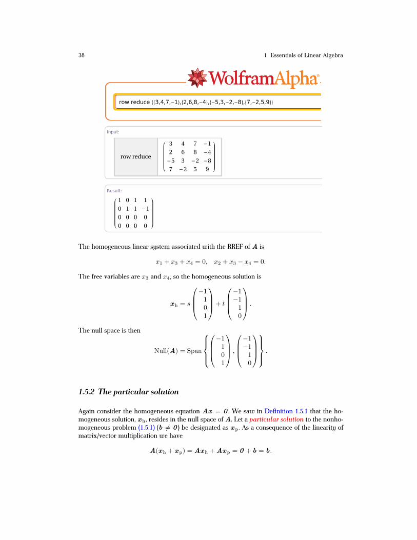
38 1 Essentials of Linear Algebra
row reduce 3,4,7,-1,2,6,8,-4,-5,3,-2,-8,7,-2,5,9
Input:
row reduce
3 4 7 -1
2 6 8 -4
-5 3 -2 -8
7 -2 5 9
Result: Step-by-step solution
1 0 1 1
0 1 1 -1
0 0 0 0
0 0 0 0
Dimensions:
4 rows ´ 4 columns
Matrix plot:
1 2 3 4
1
2
3
4
1 2 3 4
1
2
3
4
Determinant: Step-by-step solution
0
Trace:
2
Characteristic polynomial:
x4
- 2 x3
+ x2
Eigenvalues:
Λ1 � 1
Λ2 � 1
Λ3 � 0
Λ4 � 0
Generated by Wolfram|Alpha (www.wolframalpha.com) on February 12, 2015 from Champaign, IL.
© Wolfram Alpha LLC— A Wolfram Research Company1
The homogeneous linear system associated with the RREF of A is
x1 + x3 + x4 = 0, x2 + x3 − x4 = 0.
The free variables are x3 and x4, so the homogeneous solution is
xh = s
−1101
+ t
−1−110
.
The null space is then
Null(A) = Span
−1101
,
−1−110
.
1.5.2 The particular solution
Again consider the homogeneous equation Ax = 0 . We saw in Definition 1.5.1 that the ho-mogeneous solution, xh, resides in the null space of A. Let a particular solution to the nonho-mogeneous problem (1.5.1) (b 6= 0 ) be designated as xp. As a consequence of the linearity ofmatrix/vector multiplication we have
A(xh + xp) = Axh +Axp = 0 + b = b.
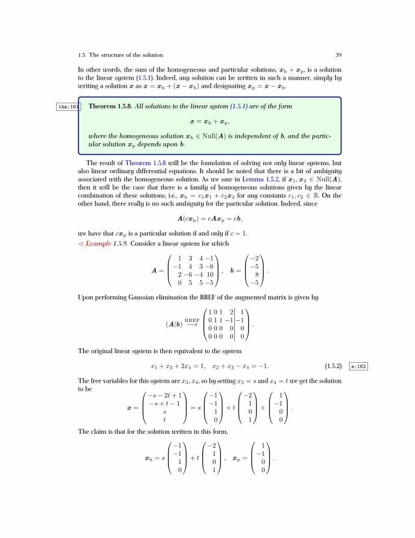
1.5 The structure of the solution 39
In other words, the sum of the homogeneous and particular solutions, xh + xp, is a solutionto the linear system (1.5.1). Indeed, any solution can be written in such a manner, simply bywriting a solution x as x = xh + (x − xh) and designating xp = x − xh.
thm:161 Theorem 1.5.8. All solutions to the linear system (1.5.1) are of the form
x = xh + xp,
where the homogeneous solution xh ∈ Null(A) is independent of b , and the partic-ular solution xp depends upon b .
The result of Theorem 1.5.8 will be the foundation of solving not only linear systems, butalso linear ordinary differential equations. It should be noted that there is a bit of ambiguityassociated with the homogeneous solution. As we saw in Lemma 1.5.2, if x 1,x 2 ∈ Null(A),then it will be the case that there is a family of homogeneous solutions given by the linearcombination of these solutions, i.e., xh = c1x 1 + c2x 2 for any constants c1, c2 ∈ R. On theother hand, there really is no such ambiguity for the particular solution. Indeed, since
A(cxp) = cAxp = cb,
we have that cxp is a particular solution if and only if c = 1.C Example 1.5.9. Consider a linear system for which
A =
1 3 4 −1−1 4 3 −62 −6 −4 100 5 5 −5
, b =
−2−58−5
.
Upon performing Gaussian elimination the RREF of the augmented matrix is given by
(A|b) RREF−→
1 0 1 2 10 1 1 −1 −10 0 0 0 00 0 0 0 0
.
The original linear system is then equivalent to the system
x1 + x3 + 2x4 = 1, x2 + x3 − x4 = −1. (1.5.2) e:162
The free variables for this system are x3, x4, so by setting x3 = s and x4 = twe get the solutionto be
x =
−s− 2t+ 1−s+ t− 1
st
= s
−1−110
+ t
−2101
+
1−100
.
The claim is that for the solution written in this form,
xh = s
−1−110
+ t
−2101
, xp =
1−100
.

40 1 Essentials of Linear Algebra
It is easy to check that xp is a particular solution,
Axp = A
1−100
=
1−120
−
34−65
=
−2−58−5
= b.
Note that xp is the last column of the RREF of the augmented matrix (A|b). Similarly, in orderto see that xh is a homogeneous solution, use the linearity of matrix/vector multiplication andcheck that
Axh = A(s
−1−110
+ t
−2101
) = sA
−1−110
+ tA
−2101
= 0 .
C Example 1.5.10. Consider the linear system Ax = b , where
A =
3 4 −7 22 6 9 −2−5 3 2 −137 −2 5 16
, b =
52711−1
.
We will use WolframAlpha to assist in finding the homogeneous and particular solutions. Webegin by computing the RREF of the augmented matrix (A|b),
row reduce 883,4,-7,2,5<,82,6,9,-2,27<,8-5,3,2,-13,11<,87,-2,5,16,-1<<
Input:
row reduce
3 4 -7 2 5
2 6 9 -2 27
-5 3 2 -13 11
7 -2 5 16 -1
Result: Step-by-step solution
1 0 0 2 0
0 1 0 -1 3
0 0 1 0 1
0 0 0 0 0
Dimensions:
4 HrowsL ´ 5 HcolumnsL
Matrix plot:
1 2 3 4 5
1
2
3
4
1 2 3 4 5
1
2
3
4
Pseudoinverse: Approximate form
1
57
13 4 -6 0
4 10 -15 0
-6 -15 51 0
22 -2 3 0
6 15 6 0
Matrix rank:
3
Generated by Wolfram|Alpha (www.wolframalpha.com) on March 27, 2014 from Champaign, IL.
© Wolfram Alpha LLC— A Wolfram Research Company1
The linear system corresponding to the RREF is
x1 + 2x4 = 0, x2 − x4 = 3, x3 = 1.
The variable x4 is the free variable, and the solution is given by
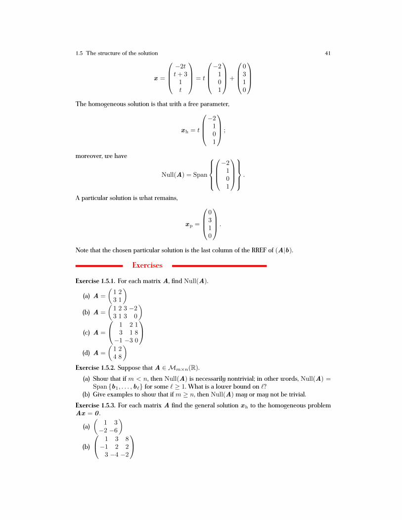
1.5 The structure of the solution 41
x =
−2tt+ 31t
= t
−2101
+
0310
The homogeneous solution is that with a free parameter,
xh = t
−2101
;
moreover, we have
Null(A) = Span
−2101
.
A particular solution is what remains,
xp =
0310
.
Note that the chosen particular solution is the last column of the RREF of (A|b).
Exercises
Exercise 1.5.1. For each matrix A, find Null(A).
(a) A =
(1 23 1
)(b) A =
(1 2 3 −23 1 3 0
)(c) A =
1 2 13 1 8−1 −3 0
(d) A =
(1 24 8
)Exercise 1.5.2. Suppose that A ∈Mm×n(R).
(a) Show that if m < n, then Null(A) is necessarily nontrivial; in other words, Null(A) =Span {b1, . . . , b`} for some ` ≥ 1. What is a lower bound on `?
(b) Give examples to show that if m ≥ n, then Null(A) may or may not be trivial.Exercise 1.5.3. For each matrix A find the general solution xh to the homogeneous problemAx = 0 .
(a)(
1 3−2 −6
)(b)
1 3 8−1 2 23 −4 −2
42 1 Essentials of Linear Algebra
(c)
−2 1 −5 −63 −2 7 114 5 17 −16
Exercise 1.5.4. For each matrix A and vector b write the solution to Ax = b as x = xh + xp,where xh is the general solution to the homogeneous problem and xp is a particular solution.Explicitly identify xh and xp.
(a)(
1 3−2 −6
), b =
(−48
)(b)
1 3 8−1 2 23 −4 −2
, b =
1004
(c)
−2 1 −5 −63 −2 7 114 5 17 −16
, b =
−8132
Exercise 1.5.5. Given the RREF of (A|b), find the general solution. Identify the homogeneoussolution, xh, and particular solution, xp.
(a)(1 0 70 1 5
)(b)
1 0 2 −30 1 −4 20 0 0 0
(c)(0 1 0 40 0 1 6
)(d)(1 0 −3 5 70 1 1 −2 9
)(e)
1 0 0 −6 20 0 1 2 −50 0 0 0 0
1.6 Equivalence results
Before continuing we wish to summarize the results we have so far proven. Moreover, we wishto connect these results to the RREF of the appropriate matrix A. We break these results intofour separate pieces.
1.6.1 A solution exists
When we defined matrix/vector multiplication so that the linear system makes sense as Ax =b , we showed that the linear system is consistent if and only if for some scalars x1, x2, . . . , xn ∈R,
b = x1a1 + x2a2 + · · ·+ xnan, A = (a1 a2 · · · an).
Using Definition 1.4.1 for the span of a collection of vectors it is then the case that the systemis consistent if and only if

1.6 Equivalence results 43
b ∈ Span {a1,a2, . . . ,an} .
On the other hand, we solve the system by using Gaussian elimination to put the augmentedmatrix (A|b) into RREF. We know that the system is inconsistent if the RREF form of theaugmented matrix has a row of the form (0 0 0 · · · 0|1); otherwise, it is consistent. These ob-servations lead to the following equivalence result:
thm:151 Theorem 1.6.1. Regarding the linear system Ax = b , where A = (a1 a2 · · · an),the following are equivalent statements:
(a) the system is consistent(b) b is a linear combination of the columns of A(c) b ∈ Span {a1,a2, . . . ,an}(d) the RREF of the augmented matrix (A|b) has no rows of the form
(0 0 0 · · · 0|1).
C Example 1.6.2. Suppose that the coefficient matrix is given by
A =
(1 23 6
).
Gaussian elimination yields that the RREF of A is
ARREF−→
(1 20 0
).
Since the RREF of A has a zero row, the system Ax = b is not consistent for all b . Since
Ax = x1
(13
)+ x2
(26
)= (x1 + 2x2)
(13
),
we have thatSpan
{(13
),
(26
)}= Span
{(13
)};
thus, Ax = b is by Theorem 1.6.1 consistent if and only if
b ∈ Span
{(13
)} b = c
(13
), c ∈ R.
In other words, the vector b must be a scalar multiple of the first column of A.
1.6.2 A solution always exists
We now wish to refine Theorem 1.6.1 in order to determine criteria which guarantee that thelinear system is consistent for any vector b . First, points (b)-(c) of Theorem 1.6.1 must be refinedto say that for any b ∈ Rm, b ∈ Span {a1, . . . ,an}; in other words, Span {a1, . . . ,an} = Rm.Additionally, for a given b no row of the RREF of the augmented matrix (A|b) has row(s) ofthe form (0 0 0 · · · 0|0). Equivalently, the RREF of A must not have a zero row. If this is thecase, then another vector b can be found such that the system will be inconsistent.
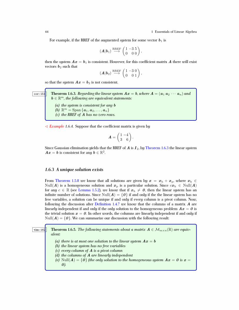
44 1 Essentials of Linear Algebra
For example, if the RREF of the augmented system for some vector b1 is
(A|b1)RREF−→
(1 −3 50 0 0
),
then the system Ax = b1 is consistent. However, for this coefficient matrix A there will existvectors b2 such that
(A|b2)RREF−→
(1 −3 00 0 1
),
so that the system Ax = b2 is not consistent.
cor:151 Theorem 1.6.3. Regarding the linear system Ax = b , where A = (a1 a2 · · · an) andb ∈ Rm, the following are equivalent statements:
(a) the system is consistent for any b(b) Rm = Span {a1,a2, . . . ,an}(c) the RREF of A has no zero rows.
C Example 1.6.4. Suppose that the coefficient matrix is given by
A =
(1 −43 6
).
Since Gaussian elimination yields that the RREF of A is I 2, by Theorem 1.6.3 the linear systemAx = b is consistent for any b ∈ R2.
1.6.3 A unique solution exists
From Theorem 1.5.8 we know that all solutions are given by x = xh + xp, where xh ∈Null(A) is a homogeneous solution and xp is a particular solution. Since cxh ∈ Null(A)for any c ∈ R (see Lemma 1.5.2), we know that if xh 6= 0 , then the linear system has aninfinite number of solutions. Since Null(A) = {0} if and only if the the linear system has nofree variables, a solution can be unique if and only if every column is a pivot column. Now,following the discussion after Definition 1.4.7 we know that the columns of a matrix A arelinearly independent if and only if the only solution to the homogeneous problem Ax = 0 isthe trivial solution x = 0 . In other words, the columns are linearly independent if and only ifNull(A) = {0}. We can summarize our discussion with the following result:
thm:162 Theorem 1.6.5. The following statements about a matrix A ∈ Mm×n(R) are equiv-alent:
(a) there is at most one solution to the linear system Ax = b(b) the linear system has no free variables(c) every column of A is a pivot column(d) the columns of A are linearly independent(e) Null(A) = {0} (the only solution to the homogeneous system Ax = 0 is x =
0 ).

1.6 Equivalence results 45
C Example 1.6.6. Suppose that
ARREF−→
1 0 −50 1 30 0 0
.
Since only the first two columns of A are pivot columns, and
Null(A) = Span
5−31
a3 = −5a1 + 3a2,
solutions to Ax = b , if they exist, cannot be unique. Moreover, since the RREF of A has a zerorow, the linear system will not always be consistent. In order for the system to be consistent, itis necessary that b ∈ Span ({a1,a2}).C Example 1.6.7. Suppose that A ∈M6×4(R) has 4 pivot columns. Since that is the maximalnumber of pivot columns, by Theorem 1.6.5 the columns are a linearly independent set. Con-sequently, the solution to a consistent linear system, Ax = b , will be unique. The columns donot form a spanning set for R6, however, since the RREF of A will have two zero rows.C Example 1.6.8. Suppose that A ∈ M3×5(R). Since A has more columns than rows, it isimpossible for the RREF of A to have a pivot position in every column. Indeed, the linear systemmust have at least two free variables, and there can be no more than three pivot columns. Hence,by Theorem 1.6.5 the columns of A cannot be linearly independent. We cannot say that thecolumns form a spanning set for R3 without knowing something more about the RREF of A. Ifwe are told that the RREF of A has two pivot positions, then the RREF of A has one zero row;hence, by Theorem 1.6.3 the columns cannot form a spanning set. However, if we are told thatthe RREF of A has three pivot positions (the maximum number possible), then the RREF of Ahas no zero rows, which by Theorem 1.6.3 means that the columns do indeed form a spanningset. In any case, the existence of free variables means that there will be an infinite number ofsolutions to any consistent linear system, Ax = b .
1.6.4 A unique solution always existss:254
We finally consider the problem of determining when there will always be a unique solutionto the linear system. By Theorem 1.6.5(c) the existence of a unique solution requires that everycolumn be a pivot column. This is possible if and only if the the linear system has no freevariables. In order for the linear system to have no free variables, the number of rows is greaterthan or equal to the number of columns. On the other hand, by Theorem 1.6.3(c) the existenceof a solution requires that the RREF of A have no zeros rows. The lack of zero rows in the RREFof A is possible if and only if the number of rows is greater than or equal to the number ofcolumns. In conclusion, we see that it is possible to always have a unique solution if and onlyif the number of rows is equal to the number of columns, i.e., if the matrix is square.
Henceforth assume that A is square. The RREF of A can have free variables if and only ifthe RREF of A has zero rows. If the RREF of A has no zero rows, then since it is square:
(a) the RREF of A is the identity matrix I n(b) the columns of A are linearly independent.
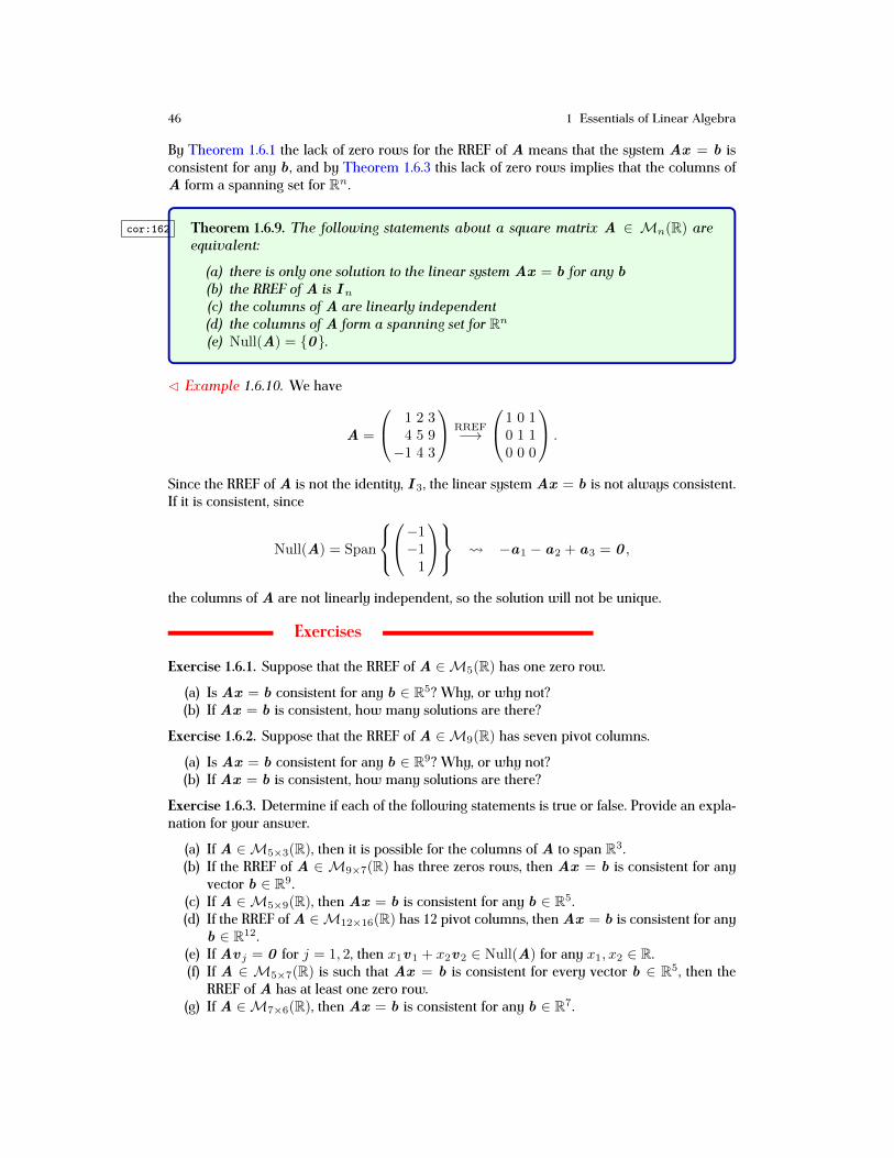
46 1 Essentials of Linear Algebra
By Theorem 1.6.1 the lack of zero rows for the RREF of A means that the system Ax = b isconsistent for any b , and by Theorem 1.6.3 this lack of zero rows implies that the columns ofA form a spanning set for Rn.
cor:162 Theorem 1.6.9. The following statements about a square matrix A ∈ Mn(R) areequivalent:
(a) there is only one solution to the linear system Ax = b for any b(b) the RREF of A is I n(c) the columns of A are linearly independent(d) the columns of A form a spanning set for Rn(e) Null(A) = {0}.
C Example 1.6.10. We have
A =
1 2 34 5 9−1 4 3
RREF−→
1 0 10 1 10 0 0
.
Since the RREF of A is not the identity, I 3, the linear system Ax = b is not always consistent.If it is consistent, since
Null(A) = Span
−1−1
1
−a1 − a2 + a3 = 0 ,
the columns of A are not linearly independent, so the solution will not be unique.
Exercises
Exercise 1.6.1. Suppose that the RREF of A ∈M5(R) has one zero row.
(a) Is Ax = b consistent for any b ∈ R5? Why, or why not?(b) If Ax = b is consistent, how many solutions are there?
Exercise 1.6.2. Suppose that the RREF of A ∈M9(R) has seven pivot columns.
(a) Is Ax = b consistent for any b ∈ R9? Why, or why not?(b) If Ax = b is consistent, how many solutions are there?
Exercise 1.6.3. Determine if each of the following statements is true or false. Provide an expla-nation for your answer.
(a) If A ∈M5×3(R), then it is possible for the columns of A to span R3.(b) If the RREF of A ∈ M9×7(R) has three zeros rows, then Ax = b is consistent for any
vector b ∈ R9.(c) If A ∈M5×9(R), then Ax = b is consistent for any b ∈ R5.(d) If the RREF of A ∈M12×16(R) has 12 pivot columns, then Ax = b is consistent for any
b ∈ R12.(e) If Av j = 0 for j = 1, 2, then x1v1 + x2v2 ∈ Null(A) for any x1, x2 ∈ R.(f) If A ∈ M5×7(R) is such that Ax = b is consistent for every vector b ∈ R5, then the
RREF of A has at least one zero row.(g) If A ∈M7×6(R), then Ax = b is consistent for any b ∈ R7.

1.6 Equivalence results 47
Exercise 1.6.4. For the given set S, determine whether the set is linearly dependent or linearlyindependent.
(a) S = {v1, v2}, where
v1 =
(3−4
), v2 =
(12
).
(b) S = {v1, v2}, where
v1 =
(2−5
), v2 =
(−410
).
(c) S = {v1, v2, v3}, where
v1 =
23−1
, v2 =
12−6
, v3 =
9157
.
(d) S = {v1, v2, v3, v4}, where
v1 =
1−20
, v2 =
3−25
, v3 =
−714
, v4 =
0−58
.
Exercise 1.6.5. Set
v1 =
1−2−5
, v2 =
−213
, v3 =
8−7r
.
(a) For which value(s) of r are the vectors v1, v2, v3 linearly independent?(b) For which value(s) of r is v3 ∈ Span {v1, v2}?(c) How are (a) and (b) related?
Exercise 1.6.6. Suppose that A ∈ M5×9(R), and further suppose the associated linear systemfor which A is the coefficient matrix has five free variables.
(a) Do the columns of A span R5? Explain.(b) Are the columns of A linearly dependent, linearly independent, or is not possible to say
without more information? Explain.
Exercise 1.6.7. Suppose that A ∈ M7×4(R), and further suppose the associated linear systemfor which A is the coefficient matrix has zero free variables.
(a) Do the columns of A span R7? Explain.(b) Are the columns of A linearly dependent, linearly independent, or is not possible to say
without more information? Explain.
Exercise 1.6.8. Suppose that A ∈ Mm×n(R). For what relationship between m and n will itbe necessarily true that:
(a) Null(A) is nontrivial.(b) the columns of A do not span Rm.
Exercise 1.6.9. Determine if each of the following statements is true or false. Provide an expla-nation for your answer.
(a) If A ∈Mm×n(R) with m > n, then the columns of A must be linearly independent.
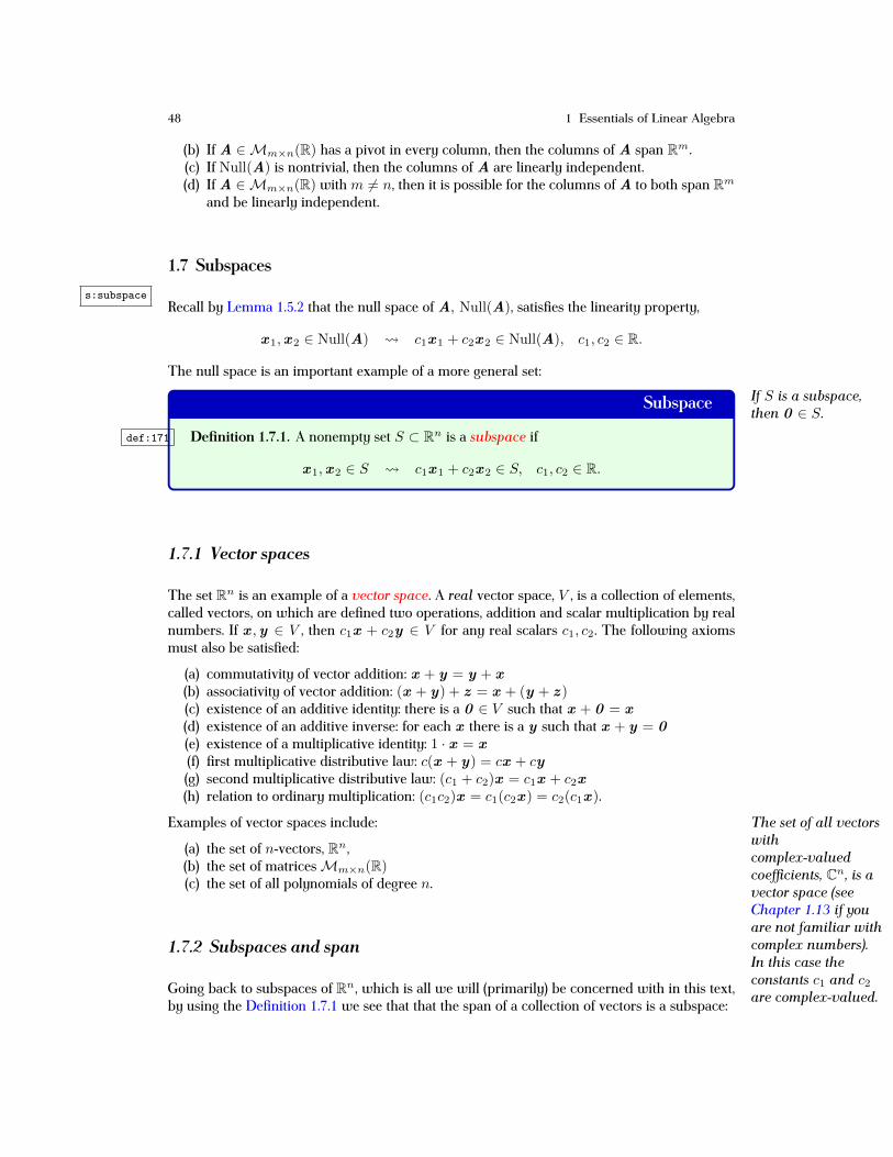
48 1 Essentials of Linear Algebra
(b) If A ∈Mm×n(R) has a pivot in every column, then the columns of A span Rm.(c) If Null(A) is nontrivial, then the columns of A are linearly independent.(d) If A ∈Mm×n(R) with m 6= n, then it is possible for the columns of A to both span Rm
and be linearly independent.
1.7 Subspacess:subspace
Recall by Lemma 1.5.2 that the null space of A, Null(A), satisfies the linearity property,
x 1,x 2 ∈ Null(A) c1x 1 + c2x 2 ∈ Null(A), c1, c2 ∈ R.
The null space is an important example of a more general set:If S is a subspace,then 0 ∈ S.Subspace
def:171 Definition 1.7.1. A nonempty set S ⊂ Rn is a subspace if
x 1,x 2 ∈ S c1x 1 + c2x 2 ∈ S, c1, c2 ∈ R.
1.7.1 Vector spaces
The set Rn is an example of a vector space. A real vector space, V , is a collection of elements,called vectors, on which are defined two operations, addition and scalar multiplication by realnumbers. If x ,y ∈ V , then c1x + c2y ∈ V for any real scalars c1, c2. The following axiomsmust also be satisfied:
(a) commutativity of vector addition: x + y = y + x(b) associativity of vector addition: (x + y) + z = x + (y + z )(c) existence of an additive identity: there is a 0 ∈ V such that x + 0 = x(d) existence of an additive inverse: for each x there is a y such that x + y = 0(e) existence of a multiplicative identity: 1 · x = x(f) first multiplicative distributive law: c(x + y) = cx + cy(g) second multiplicative distributive law: (c1 + c2)x = c1x + c2x(h) relation to ordinary multiplication: (c1c2)x = c1(c2x ) = c2(c1x ).
The set of all vectorswithcomplex-valuedcoefficients, Cn, is avector space (seeChapter 1.13 if youare not familiar withcomplex numbers).In this case theconstants c1 and c2are complex-valued.
Examples of vector spaces include:
(a) the set of n-vectors, Rn,(b) the set of matricesMm×n(R)(c) the set of all polynomials of degree n.
1.7.2 Subspaces and span
Going back to subspaces of Rn, which is all we will (primarily) be concerned with in this text,by using the Definition 1.7.1 we see that that the span of a collection of vectors is a subspace:

1.7 Subspaces 49
lem:171 Lemma 1.7.2. The set S = Span {a1,a2, . . . ,ak} is a subspace.
Proof. Suppose that b1, b2 ∈ S. By Lemma 1.4.2 there exist vectors x 1,x 2 such that for A =(a1 a2 · · · ak),
Ax 1 = b1, Ax 2 = b2.
We must now show that for the vector b = c1b1 + c2b2 there is a vector x such that Ax = b ,as it will then be true that b ∈ S. However, if we choose x = c1x 1+ c2x 2, then by the linearityof matrix/vector multiplication we have that
Ax = A(c1x 1 + c2x 2) = c1Ax 1 + c2Ax 2 = c1b1 + c2b2 = b. ut
The converse also holds. It can be shown that any subspace of Rn is realized as the span ofsome finite collection of vectors in Rn (see Lemma 1.8.16). In other words, in the vector spaceRn there are no other subspaces other than those given in Lemma 1.7.2.
lem:171a Theorem 1.7.3. S ⊂ Rn is a subspace if and only if there is a collection of vectors{a1,a2, . . . ,ak} such that S = Span {a1,a2, . . . ,ak}.
C Example 1.7.4. Suppose that
S =
x1 + 2x2−3x2
4x1 + x2
: x1, x2 ∈ R
.
Since x1 + 2x2−3x2
4x1 + x2
= x1
104
+ x2
2−31
= Span
1
04
,
2−31
,
by Theorem 1.7.3 the set is a subspace.C Example 1.7.5. Suppose that
S =
x1 + 2x2
1− 3x24x1 + x2
: x1, x2 ∈ R
.
We have that b ∈ S if and only if
b =
010
+ x1
104
+ x2
2−31
.
If S is a subspace, then it must contain the zero vector. Writing
0 =
010
+ x1
104
+ x2
2−31
=
010
+
1 20 −34 1
(x1x2
),
upon using
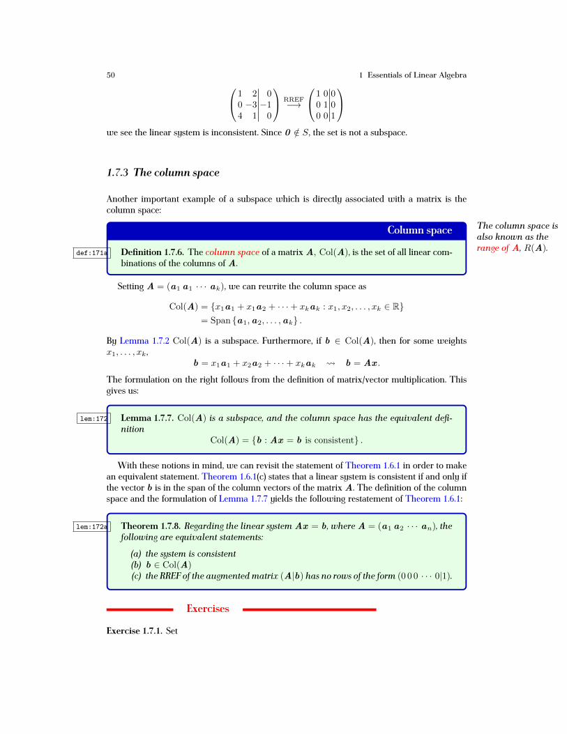
50 1 Essentials of Linear Algebra 1 2 00 −3 −14 1 0
RREF−→
1 0 00 1 00 0 1
we see the linear system is inconsistent. Since 0 /∈ S, the set is not a subspace.
1.7.3 The column space
Another important example of a subspace which is directly associated with a matrix is thecolumn space:
The column space isalso known as therange of A, R(A).
Column space
def:171a Definition 1.7.6. The column space of a matrix A, Col(A), is the set of all linear com-binations of the columns of A.
Setting A = (a1 a1 · · · ak), we can rewrite the column space as
Col(A) = {x1a1 + x1a2 + · · ·+ xkak : x1, x2, . . . , xk ∈ R}= Span {a1,a2, . . . ,ak} .
By Lemma 1.7.2 Col(A) is a subspace. Furthermore, if b ∈ Col(A), then for some weightsx1, . . . , xk ,
b = x1a1 + x2a2 + · · ·+ xkak b = Ax .
The formulation on the right follows from the definition of matrix/vector multiplication. Thisgives us:
lem:172 Lemma 1.7.7. Col(A) is a subspace, and the column space has the equivalent defi-nition
Col(A) = {b : Ax = b is consistent} .
With these notions in mind, we can revisit the statement of Theorem 1.6.1 in order to makean equivalent statement. Theorem 1.6.1(c) states that a linear system is consistent if and only ifthe vector b is in the span of the column vectors of the matrix A. The definition of the columnspace and the formulation of Lemma 1.7.7 yields the following restatement of Theorem 1.6.1:
lem:172a Theorem 1.7.8. Regarding the linear system Ax = b , where A = (a1 a2 · · · an), thefollowing are equivalent statements:
(a) the system is consistent(b) b ∈ Col(A)(c) the RREF of the augmented matrix (A|b) has no rows of the form (0 0 0 · · · 0|1).
Exercises
Exercise 1.7.1. Set

1.7 Subspaces 51
S =
2s− 3t−s+ 4t
7t
: s, t ∈ R
⊂ R3.
Is S a subspace? If so, determine vectors x 1,x 2, . . . ,xk such that S = Span {x 1,x 2, . . . ,xk}.Otherwise, explain why S is not a subspace.Exercise 1.7.2. Set
S =
4s+ 2t
1− 3s− ts+ 9t
: s, t ∈ R
⊂ R3.
Is S a subspace? If so, determine vectors x 1,x 2, . . . ,xk such that S = Span {x 1,x 2, . . . ,xk}.Otherwise, explain why S is not a subspace.
hw:263 Exercise 1.7.3. Let A,B ⊂ Rn be subspaces, and define
A+B = {x : x = a + b, a ∈ A, b ∈ B} .
Show that A + B is a subspace. (Hint: use the fact that set is a subspace if and only if it is thespan of a collection of vectors)Exercise 1.7.4. If
A =
(−4 7 03 5 1
), b =
(−65
),
is b ∈ Col(A)? Explain your answer.Exercise 1.7.5. If
A =
3 −12 7−4 9
, b =
24−1
,
is b ∈ Col(A)? Explain your answer.Exercise 1.7.6. If
A =
5 2 −3−4 9 02 6 −7
, b =
−582
,
is b ∈ Col(A)? Explain your answer.Exercise 1.7.7. Set
A =
1 −32 5−1 4
, u =
2−47
, v =
−3165
.
(a) Is u ∈ Col(A)? Explain.(b) Is v ∈ Col(A)? Explain.(c) Describe all vectors that belong to Col(A) as the span of a finite set of vectors.
Exercise 1.7.8. Show that the set of 2× 2 matrices,M2(R), is a vector space.Exercise 1.7.9. Consider the set of matrices inM2(R) given by
S =
{A =
(a bc d
): a+ d = 0
}.

52 1 Essentials of Linear Algebra
Show that S is a subspace. (Hint: find a set of matrices such that any A ∈ S can be written asa linear combination of these matrices)Exercise 1.7.10. Show that the set of third-order polynomials,
P3(R) = {a0 + a1t+ a2t2 + a3t
3 : a0, . . . , a3 ∈ R},
is a vector space.Exercise 1.7.11. Consider the set of polynomials in P3(R) given by
S = {p ∈ P3(R) : p′(1) = 0} .
Show that S is a subspace. (Hint: find a set of polynomials such that any p ∈ S can be writtenas a linear combination of these polynomials)
1.8 Basis and dimensions:272
1.8.1 Basis
The next question to consider is the “size” of a subspace. The number that we assign to the “size”should reflect the intuition that a plane in R3 is bigger than a line in R3, and hence the numberassigned to a plane should be larger than the number associated with the line. Regarding agiven plane going through the origin in R3, while the geometric object itself is unique, there aremany ways to describe it. For example, in Calculus we learned that it can be described as beingthe set of all vectors which are perpendicular to a certain vector. Conversely, we could describeit as the span of a collection of vectors which lie in the plane. The latter notion is the one thatwe will use, as it more easily generalizes to higher dimensions. One way to determine the “size”of the subspace is to then count the number of spanning vectors. Because an arbitrarily highnumber of vectors could be used as the spanning set, in order to uniquely determine the size ofthe space we must restrict the possible number of spanning vectors as much as possible. Thisrestriction requires that we use only the linearly independent vectors (see Definition 1.4.7) inthe spanning set. We first label these vectors:
Basisdef:172 Definition 1.8.1. A set B = {a1,a2, . . . ,ak} is a basis for a subspace S if
(a) the vectors a1,a2, . . . ,ak are linearly independent(b) S = Span {a1,a2, . . . ,ak}.
In other words, the set of vectors is a basis if(a) any vector in S can be written as a linear combination of the basis vectors(b) there are not so many vectors in the set that (at least) one of them can be written as a
linear combination of the others.C Example 1.8.2. We wish to find a basis for the column space, Col(A), of the matrix
A =
−2 3 −13 −5 16 −7 5
.

1.8 Basis and dimension 53
Since
ARREF−→
1 0 20 1 10 0 0
,
we have
Null(A) = Span
−2−1
1
a3 = 2a1 + a2.
Consequently, regarding the column space we have
Col(A) = Span
−23
6
,
3−5−7
.
These first two columns are clearly linearly independent. In conclusion, these two pivotcolumns are a basis for Col(A).
The previous example, as well as the several examples we did in Chapter 1.4, point us to-wards a general truth. In all these examples a set of linearly independent vectors in the set ofcolumn vectors, {a1,a2, . . . ,ak}, which form a spanning set for Col(A) were found by re-moving from the original set those columns which correspond to free variables for associatedhomogeneous linear system. In other words, a set of linearly independent vectors which whichspan the column space is the collection of pivot columns. In general, it is a relatively straightfor-ward exercise (see Exercise 1.8.12) to show that each column of a matrix A which is not a pivotcolumn can be written as a linear combination of the pivot columns. Thus, by the definition ofbasis we have:
ex:column Lemma 1.8.3. The pivot columns of A ∈ Mm×n(R) form a basis for the columnspace, Col(A).
C Example 1.8.4. Let
a1 =
1−12
, a2 =
347
, a3 =
0−7−1
,
and set S = {a1,a2,a3}. It can be checked that
A = (a1 a2 a3)RREF−→
1 0 30 1 −10 0 0
.
The first and second columns of A are the pivot columns, so
Span {a1,a2,a3} = Span {a1,a2} .
Since
Null(A) = Span
−31
1
,
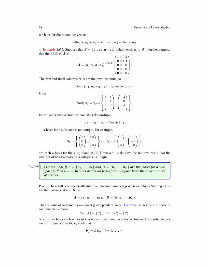
54 1 Essentials of Linear Algebra
we have for the remaining vector,
−3a1 + a2 + a3 = 0 a3 = 3a1 − a2.
C Example 1.8.5. Suppose that S = {a1,a2,a3,a4}, where each aj ∈ R5. Further supposethat the RREF of A is
A = (a1 a2 a3 a4)RREF−→
1 1 0 30 0 1 40 0 0 00 0 0 00 0 0 0
.
The first and third columns of A are the pivot columns, so
Span {a1,a2,a3,a4} = Span {a1,a3} .
Since
Null(A) = Span
−1100
,
−30−41
,
for the other two vectors we have the relationships,
a2 = a1, a4 = 3a1 + 4a3.
A basis for a subspace is not unique. For example,
B1 =
1
00
,
010
, B2 =
1
10
,
1−10
,
are each a basis for the x1x2-plane in R3. However, we do have the intuitive result that thenumber of basis vectors for a subspace is unique.
lem:173 Lemma 1.8.6. If A = {a1, . . . ,ak} and B = {b1, . . . , bm} are two bases for a sub-space S, then k = m. In other words, all bases for a subspace have the same numberof vectors.
Proof. The result is geometrically intuitive. The mathematical proof is as follows. Start by form-ing the matrices A and B via
A = (a1 a2 · · · ak), B = (b1 b2 · · · bm).
The columns of each matrix are linearly independent, so by Theorem 1.6.5(e) the null space ofeach matrix is trivial,
Null(A) = {0} , Null(B) = {0} .
Since A is a basis, each vector in B is a linear combination of the vectors in A; in particular, foreach bj there is a vector cj such that
bj = Acj , j = 1, . . . ,m.

1.8 Basis and dimension 55
If we setC = (c1 c2 · · · cm) ∈Mk×m(R),
the matrices A and B are then related by
B = (b1 b2 · · · bm) = (Ac1 Ac2 · · · Acm) = AC .
Suppose that s ∈ S. Since A and B are each a basis there exist unique vectors xA and xBsuch that
s = AxA = BxB .
But, the relation B = AC implies that
AxA = (AC )xB = A(CxB) A(xA −CxB) = 0
(the last implicated equality follows from the linearity of matrix/matrix multiplication). Recallingthat Null(A) = {0}, xA and xB are related via
A(xA −CxB) = 0 xA −CxB = 0 xA = CxB .
Finally, consider the linear system Cx = y . For a given y = xA, there is a unique solu-tion x = xB . This follows simply from the fact that for a given vector s ∈ S there are thecorresponding vectors xA and xB , and these are related through matrix/vector multiplication,xA = CxB . Since the linear system always has a unique solution, we know from our discus-sion leading to Theorem 1.6.9 that the matrix C must be square. Thus, k = m, which is thedesired result. ut
1.8.2 Dimension and ranks:172
Because the number of vectors in a basis of a subspace is fixed, this quantity gives a good wayto describe the “size” of a subspace.
Dimensiondef:173 Definition 1.8.7. If B = {a1,a2, . . . ,ak} is a basis for a subspace S, then the dimen-
sion of S, dim[S], is the number of basis vectors:
dim[S] = k.dim[{0}] = 0
example:basis C Example 1.8.8. Let ej for j = 1, . . . , n denote the jth column vector in the identity matrixI n. Since I n is in RREF, by Theorem 1.6.9 the set {e1, e2, . . . , en} is linearly independent andforms a spanning set for Rn; in other words, it is a basis for Rn. By Definition 1.8.7 we thenhave the familiar result that dim[Rn] = n.
Regarding the dimension of the column space, we use the following moniker:

56 1 Essentials of Linear Algebra
Rankdef:173a Definition 1.8.9. The dimension of the column space of a matrix is known as the rank,
rank(A) = dim[Col(A)].
1
0
1
1
00
00
0
free variable columnspivot columns
Fig. 1.2 (color online) A cartoon of a matrix in RREF. A vertical (blue) line represents a column associ-ated with a free variable. The remaining columns are pivot columns. f:rank
We now relate the column space to the null space through their dimensions. The pivotcolumns of the RREF of A are a basis for Col(A) (see Lemma 1.8.3), so
rank(A) = # of pivot columns.
In addition, the number of free variables is the number of linearly independent vectors thatform a spanning set for Null(A). Consequently, we can say
dim[Null(A)] = # of free variables.
Since a column of the RREF of A is either a pivot column, or is associated with a free variable(see Figure 1.2), upon using the fact that sum of the number of pivot columns and the numberof free variables is the total number of columns, we get:
lem:174 Lemma 1.8.10. For the matrix A ∈Mm×n(R),
rank(A) + dim[Null(A)] = n.
The dimension of the column space gives us one more bit of information. Suppose thatA ∈ Mm×n(R), so that Col(A) ⊂ Rm. Upon invoking a paraphrase of Theorem 1.6.3, weknow that Ax = b is consistent for any b ∈ Rm if and only if the RREF of A has precisely mpivot columns. In other words, the system is consistent for any b if and only if
rank(A) = dim[Rm] = m ⇔ dim[Null(A)] = n−m.

1.8 Basis and dimension 57
If rank(A) ≤ m− 1, then it will necessarily be the case that Ax = b will not be consistent forall b . For example, if A ∈ M3(R) and rank(A) = 2, then it will be the case that the subspaceCol(A) is a plane, and the linear system Ax = b will be consistent if and only if the vector bis parallel to that plane.
We now restate the equivalency Theorem 1.6.3 and equivalency Theorem 1.6.5. The firsttheorem discusses conditions which ensure that a linear system always has a unique solution:
If any of theequivalentconditions
Theorem 1.8.11(a)-(c)hold, then A is said
to have full rank.
thm:171 Theorem 1.8.11. The following statements about a matrixMm×n(R) are equivalent:
(a) the linear system Ax = b is consistent for any b(b) dim[Null(A)] = n−m(c) rank(A) = m.
This next result gives conditions which ensure that consistent systems have unique solutions:
thm:171aa Theorem 1.8.12. The following statements about a matrixMm×n(R) are equivalent:
(a) there is at most one solution to the linear system Ax = b(b) dim[Null(A)] = 0(c) rank(A) = n.
If we wish that the linear system Ax = b be both consistent for all b , and to have onlyunique solutions, then we saw in Chapter 1.6.4 that this is possible only if A is a square matrix,i.e., m = n. If the solution is to be unique, then by Theorem 1.8.11(b) we must have
dim[Null(A)] = 0.
If the linear system is to be consistent, then by Theorem 1.8.12(c) the rank of the matrix mustbe the number of rows, i.e.,
rank(A) = n.
In terms of dimensions we can then restate Theorem 1.6.9 to say:
thm:163 Theorem 1.8.13. Consider the linear system Ax = b , where A ∈ Mn(R). The fol-lowing statements are equivalent:
(a) there is a unique solution to the linear system for any b(b) rank(A) = n(c) dim[Null(A)] = 0.
C Example 1.8.14. Suppose that
A =
1 3 −2 11 −1 2 13 4 −1 1
RREF−→
1 0 1 00 1 −1 00 0 0 1
.
Since the pivot columns are the first, second, and fourth columns of the RREF of A, a basis forCol(A) is given by the set
113
,
3−14
,
111
.

58 1 Essentials of Linear Algebra
Since rank(A) = 3 = dim[R3], the linear system Ax = b is consistent for any b ∈ R3. Sincedim[Null(A)] = 1 > 0, the solutions are not unique.C Example 1.8.15. We now compute Col(A) and Null(A) with the assistance of WolframAl-pha. Here A ∈M4(R) is given by
A =
1 2 3 4−1 2 1 05 6 11 162 4 6 8
.
We start with
row reduce 881,2,3,4<,8-1,2,1,0<,85,6,11,16<,82,4,6,8<<
Input:
row reduce
1 2 3 4
-1 2 1 0
5 6 11 16
2 4 6 8
Result: Step-by-step solution
1 0 1 2
0 1 1 1
0 0 0 0
0 0 0 0
Dimensions:
4 HrowsL ´ 4 HcolumnsL
Matrix plot:
1 2 3 4
1
2
3
4
1 2 3 4
1
2
3
4
Determinant: Step-by-step solution
0
Trace:
2
Characteristic polynomial:
x4
- 2 x3
+ x2
Eigenvalues:
Λ1 � 1
Λ2 � 1
Λ3 � 0
Λ4 � 0
Generated by Wolfram|Alpha (www.wolframalpha.com) on February 12, 2015 from Champaign, IL.
© Wolfram Alpha LLC— A Wolfram Research Company1
Since there are two pivot columns and two columns associated with free variables, rank(A) =2, and dim[Null(A)] = 2. Since rank(A) < dim[R4] = 4, the linear system will not necessarilybe consistent. Since dim[Null(A)] ≥ 1, if the system is consistent, there will be an infinitenumber of solution.
A basis for Col(A) is the pivot columns of A, which are the first two columns,
Col(A) = Span
1−152
,
2264
.
As for the null space, the homogeneous linear system associated with the RREF of A is
x1 + x3 + 2x4 = 0, x2 + x3 + x4 = 0.
Since x3 and x4 are the free variables, the homogeneous solution is
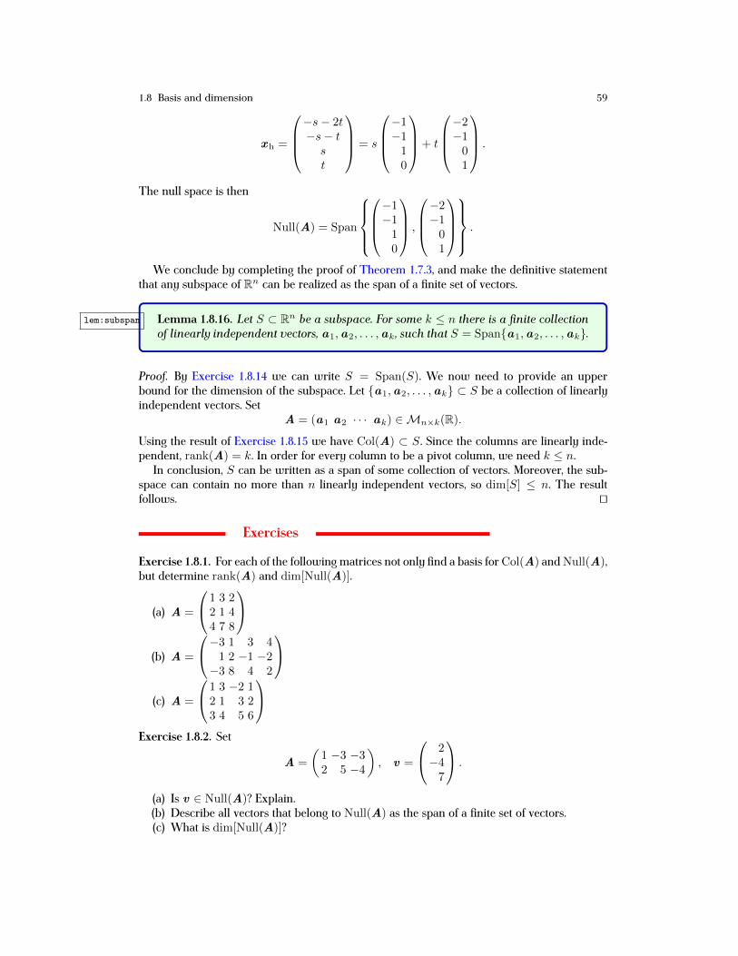
1.8 Basis and dimension 59
xh =
−s− 2t−s− tst
= s
−1−110
+ t
−2−101
.
The null space is then
Null(A) = Span
−1−110
,
−2−101
.
We conclude by completing the proof of Theorem 1.7.3, and make the definitive statementthat any subspace of Rn can be realized as the span of a finite set of vectors.
lem:subspan Lemma 1.8.16. Let S ⊂ Rn be a subspace. For some k ≤ n there is a finite collectionof linearly independent vectors, a1,a2, . . . ,ak , such that S = Span{a1,a2, . . . ,ak}.
Proof. By Exercise 1.8.14 we can write S = Span(S). We now need to provide an upperbound for the dimension of the subspace. Let {a1,a2, . . . ,ak} ⊂ S be a collection of linearlyindependent vectors. Set
A = (a1 a2 · · · ak) ∈Mn×k(R).
Using the result of Exercise 1.8.15 we have Col(A) ⊂ S. Since the columns are linearly inde-pendent, rank(A) = k. In order for every column to be a pivot column, we need k ≤ n.
In conclusion, S can be written as a span of some collection of vectors. Moreover, the sub-space can contain no more than n linearly independent vectors, so dim[S] ≤ n. The resultfollows. ut
Exercises
Exercise 1.8.1. For each of the following matrices not only find a basis for Col(A) and Null(A),but determine rank(A) and dim[Null(A)].
(a) A =
1 3 22 1 44 7 8
(b) A =
−3 1 3 41 2 −1 −2−3 8 4 2
(c) A =
1 3 −2 12 1 3 23 4 5 6
Exercise 1.8.2. Set
A =
(1 −3 −32 5 −4
), v =
2−47
.
(a) Is v ∈ Null(A)? Explain.(b) Describe all vectors that belong to Null(A) as the span of a finite set of vectors.(c) What is dim[Null(A)]?

60 1 Essentials of Linear Algebra
Exercise 1.8.3. Suppose that A ∈M7×8(R). If:
(a) the RREF of A has two zero rows, what is rank(A)?(b) A has 5 pivot columns, what is dim[Null(A)]?
Exercise 1.8.4. Can a set of eight vectors be a basis for R7? Explain.Exercise 1.8.5. Can a set of five vectors be a basis for R6? Explain.Exercise 1.8.6. Is the set
S =
{(15
),
(−23
)}a basis for R2? Explain. If not, find a basis for Span(S), and determine dim[Span(S)].Exercise 1.8.7. Is the set
S =
1
5−2
,
−230
,
31−5
a basis for R3? Explain. If not, find a basis for Span(S), and determine dim[Span(S)].Exercise 1.8.8. Is the set
S =
1
13
,
−214
,
412
a basis for R3? Explain. If not, find a basis for Span(S), and determine dim[Span(S)].Exercise 1.8.9. Set
A =
1 2 5−1 5 22 −7 −1
, b =
813−17
.
(a) Find a basis for Col(A).(b) What is rank(A)?(c) The vector b ∈ Col(A). Write the vector as a linear combination of the basis vectors
chosen in part (a).
Exercise 1.8.10. Set
A =
1 −3 −2 02 −6 1 5−1 3 3 1−3 9 1 −5
, b =
−5580
.
(a) Find a basis for Col(A).(b) What is rank(A)?(c) The vector b ∈ Col(A). Write the vector as a linear combination of the basis vectors
chosen in part (a).
Exercise 1.8.11. Determine if each of the following statements is true or false. Provide an ex-planation for your answer.
(a) If A ∈M7(R) is such that the RREF of A has two zero rows, then rank(A) = 6.(b) Any set of seven linearly independent vectors is a basis for R7.(c) If A ∈M4×6(R) is such that the RREF of A has one zero row, then dim[Null(A)] = 4.(d) If A ∈M9(R) is such that the RREF of A has six pivot columns, dim[Null(A)] = 3.
hw:linind Exercise 1.8.12. Let S = {a1,a2, . . . ,ak} be a set of vectors, and set A = (a1 a2 · · · ak).

1.9 Inner-products and orthogonal bases 61
(a) Show that each column of A which is not a pivot column can be written as a linearcombination of the pivot columns (Hint: consider Null(A)).
(b) Prove Lemma 1.8.3.
Exercise 1.8.13. Let {a1,a2, . . . ,ak} ⊂ Rn be a linearly independent set of vectors. Set Sj =Span{a1,a2, . . . ,aj} for j = 1, 2, . . . , k.
(a) Show that dim[Sj ] = j for each j = 1, 2, . . . , k.(b) Show that S1 ⊂ S2 ⊂ · · · ⊂ Sk .
hw:subspace2 Exercise 1.8.14. Let S ⊂ Rn be a subspace. Show that S = Span(S), where we define the spanof a subspace to be the set of all finite linear combinations of vectors in S.
hw:subspace1 Exercise 1.8.15. Let {a1,a2, . . . ,ak} ⊂ S, where S ⊂ Rn is a subspace. Show that
Span{a1,a2, . . . ,ak} ⊂ S.
hw:dimsubspace Exercise 1.8.16. Let S1, S2 ⊆ Rn be subspaces with S1 ⊆ S2. Show that dim[S1] ≤ dim[S2].(Hint: Find a basis for S1 and S2)
1.9 Inner-products and orthogonal basess:ip18
In Calculus we introduced the dot product of two vectors in order to compute the angle betweenthem. We generalize this notion to vectors of any size, and call it an inner-product. Using aninner-product we show that by taking a special set of vectors for a basis it is straightforward towrite a given vector as a linear combination of the basis vectors. Moreover, we give an algorithmfor constructing such a basis.
1.9.1 The inner-product on Rn
The dot product of two vectors x ,y ∈ R3 is given by
x · y =
3∑j=1
xjyj = x1y1 + x2y2 + x3y3.
The natural generalization to vectors in Rn is:
Inner-product
def:innerproduct Definition 1.9.1. An inner-product on Rn is given by
〈x ,y〉 =n∑j=1
xjyj = x1y1 + x2y2 + · · ·+ xnyn.
The inner-product of two vectors has the same properties as the dot product:
(a) 〈x ,y〉 = 〈y ,x 〉(b) 〈x ,x 〉 ≥ 0 with equality if and only if x = 0

62 1 Essentials of Linear Algebra
(c) 〈x + y , z 〉 = 〈x , z 〉+ 〈y , z 〉(d) 〈cx ,y〉 = 〈x , cy〉 = c〈x ,y〉 for any c ∈ R
The proof of these properties is left as an exercise in Exercise 1.9.1. Properties (c) and (d) guar-antee that the inner product is a linear operation (see Exercise 1.9.2). Property (b) allows us todefine the length (magnitude) of a vector by
‖x‖2 := 〈x ,x 〉.
The length has the properties
(a) ‖cx‖ = |c| ‖x‖ for any c ∈ R(b) ‖x + y‖ ≤ ‖x‖+ ‖y | (the triangle inequality)
(see Exercise 1.9.3). A unit vector has length one,
〈x ,x 〉 = ‖x‖2 = 1.
If x is a nonzero vector, then u = x/‖x‖ is a unit vector which points in the same direction asx (see Exercise 1.9.4).
x
y
x-y
θ
Fig. 1.3 (color online) A cartoon for the relationship between the vectors x , y , and x − y . f:VectorAngle
C Example 1.9.2. If
x =
123
, y =
0−14
, z =
215
,
then〈x ,y〉 = 10, 〈x , z 〉 = 19, 〈y , z 〉 = 19.
Using linearity,〈2x − 3y , z 〉 = 2〈x ,x 〉 − 3〈y , z 〉 = 20− 57 = −37.
Since 〈x ,x 〉 = 14, a unit vector pointing in the same direction as x is
u =1√14
x =
1/√14
2/√14
3/√14
.
As is the case with the dot product, the inner-product can be used to determine the anglebetween two vectors (see Figure 1.3). We start by using linearity to say

1.9 Inner-products and orthogonal bases 63
〈x − y ,x − y〉 = 〈x ,x 〉 − 〈y ,x 〉 − 〈x ,y〉+ 〈y ,y〉= 〈x ,x 〉 − 2〈x ,y〉+ 〈y ,y〉.
The second line follows from property (a). Using the definition of a length of a vector we canrewrite the above as
‖x − y‖2 = ‖x‖2 + ‖y‖2 − 2〈x ,y〉.
Now, if we think of the three vectors x ,y ,x −y as forming three legs of a triangle, then by thelaw of cosines we have
‖x − y‖2 = ‖x‖2 + ‖y‖2 − 2‖x‖ ‖y‖ cos θ,
where θ is the angle between x and y . Comparing the two equations reveals:
Bessel’s inequality
prop:vecangle Proposition 1.9.3. The angle between two vectors x ,y ∈ Rn is determined by
〈x ,y〉 = ‖x‖ ‖y‖ cos θ.
In particular, we have Bessel’s inequality,
|〈x ,y〉| ≤ ‖x‖ ‖y‖.
Proof. Bessel’s inequality follows immediately from the first equality upon noting | cos θ| ≤1. ut
If the inner-product between two vectors is zero, we say:
Orthogonal
def:orthogonal Definition 1.9.4. The two vectors x ,y ∈ Rn are orthogonal (perpendicular) if
〈x ,y〉 = 0.
1.9.2 Orthonormal bases
Consider a collection of nonzero vectors {a1,a2, . . . ,ak}, and suppose that the vectors aremutually orthogonal,
〈a i,aj〉 = 0, i 6= j.
We first show that the vectors must be linearly independent. Going back to the original Def-inition 1.4.7, this means that we must show that the only solution to the homogeneous linearsystem,
x1a1 + x2a2 + · · ·+ xkak = 0 ,
is x1 = x2 = · · · = xk = 0.For a given vector y take the inner-product to both sides,

64 1 Essentials of Linear Algebra
〈x1a1 + x2a2 + · · ·+ xkak,y〉 = 〈0 ,y〉.
Now use the linearity of the inner-product to rewrite the above as one linear equation,
x1〈a1,y〉+ x2〈a2,y〉+ · · ·+ xk〈ak,y〉 = 0. (1.9.1) e:ip1
This is one linear equation in k variables; however, we have some freedom in choosing thecoefficients by choosing different vectors y .
If we choose y = a1 in (1.9.1), then upon using the fact that the vectors are mutually orthog-onal the equation reduces to
x1〈a1,a1〉 = 0.
Since the vectors being nonzero implies 〈a1,a1〉 = ‖a1‖2 > 0, we can conclude x1 = 0; thus,(1.9.1) can be rewritten as
x2〈a2,y〉+ x3〈a3,y〉+ · · ·+ xk〈ak,y〉 = 0. (1.9.2) e:ip2
If we choose y = a2 in (1.9.2), then the mutual orthogonality of the vectors yields the reducedequation
x2〈a2,a2〉 = 0.
Since all of the vectors are nonzero we conclude x2 = 0. Continuing in this fashion leads tox3 = x4 = · · · = xk = 0. We conclude:
lem:orthlinind Lemma 1.9.5. Suppose the nonzero vectors {a1,a2, . . . ,ak} are mutually orthogo-nal,
〈a i,aj〉 = 0, i 6= j.
The set of vectors is then linearly independent.
While a basis for a subspace is not unique, the dimension is fixed. As we will soon see, anespecially useful basis is:
Orthonormal basisdef:orthonormal Definition 1.9.6. The set of vectors {u1,u2, . . . ,uk} forms an orthonormal basis for
a subspace S if
(a) S = Span {u1,u2, . . . ,uk}
(b) 〈u i,uj〉 =
{0, i 6= j
1, i = j.
In other words, the basis vectors are mutually orthogonal, and each has length one.
C Example 1.9.7. Suppose S = Span{a1,a2,a3}, where
a1 =
123
, a2 =
−301
, a3 =
1−53
.
The vectors are clearly mutually orthogonal. Setting
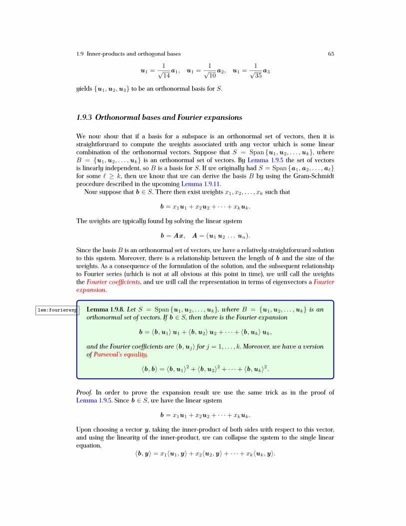
1.9 Inner-products and orthogonal bases 65
u1 =1√14
a1, u1 =1√10
a2, u1 =1√35
a3
yields {u1,u2,u3} to be an orthonormal basis for S.
1.9.3 Orthonormal bases and Fourier expansions
We now show that if a basis for a subspace is an orthonormal set of vectors, then it isstraightforward to compute the weights associated with any vector which is some linearcombination of the orthonormal vectors. Suppose that S = Span {u1,u2, . . . ,uk}, whereB = {u1,u2, . . . ,uk} is an orthonormal set of vectors. By Lemma 1.9.5 the set of vectorsis linearly independent, so B is a basis for S. If we originally had S = Span {a1,a2, . . . ,a`}for some ` ≥ k, then we know that we can derive the basis B by using the Gram-Schmidtprocedure described in the upcoming Lemma 1.9.11.
Now suppose that b ∈ S. There then exist weights x1, x2, . . . , xk such that
b = x1u1 + x2u2 + · · ·+ xkuk.
The weights are typically found by solving the linear system
b = Ax , A = (u1 u2 . . . un).
Since the basisB is an orthonormal set of vectors, we have a relatively straightforward solutionto this system. Moreover, there is a relationship between the length of b and the size of theweights. As a consequence of the formulation of the solution, and the subsequent relationshipto Fourier series (which is not at all obvious at this point in time), we will call the weightsthe Fourier coefficients, and we will call the representation in terms of eigenvectors a Fourierexpansion.
lem:fourierexp Lemma 1.9.8. Let S = Span {u1,u2, . . . ,uk}, where B = {u1,u2, . . . ,uk} is anorthonormal set of vectors. If b ∈ S, then there is the Fourier expansion
b = 〈b,u1〉u1 + 〈b,u2〉u2 + · · ·+ 〈b,uk〉uk,
and the Fourier coefficients are 〈b,uj〉 for j = 1, . . . , k. Moreover, we have a versionof Parseval’s equality,
〈b, b〉 = 〈b,u1〉2 + 〈b,u2〉2 + · · ·+ 〈b,uk〉2.
Proof. In order to prove the expansion result we use the same trick as in the proof ofLemma 1.9.5. Since b ∈ S, we have the linear system
b = x1u1 + x2u2 + · · ·+ xkuk.
Upon choosing a vector y , taking the inner-product of both sides with respect to this vector,and using the linearity of the inner-product, we can collapse the system to the single linearequation,
〈b,y〉 = x1〈u1,y〉+ x2〈u2,y〉+ · · ·+ xk〈uk,y〉.

66 1 Essentials of Linear Algebra
If we take y = u1, then upon using the fact that the vectors are orthonormal,
〈u i,uj〉 =
{0, i 6= j
1, i = j,
the equation becomes〈b,u1〉 = x1 · 1.
If we take y = u2, then the equation becomes
〈b,u2〉 = x2 · 1.
Continuing in this fashion leads to the desired result,
xj = 〈b,uj〉, j = 1, . . . , k.
Regarding Parseval’s equality, this follows immediately upon taking the inner product ofboth sides of the Fourier expansion with b , and using the linearity of the inner product. Thedetails are left for the interested student (see Exercise 1.9.5). ut
ex:gs1 C Example 1.9.9. Suppose S = Span {u1,u2}, where
u1 =1√14
123
, u2 =1√13
03−2
.
It is easy to check that {u1,u2} is an orthonormal basis for S. Now suppose
b =
18−1
∈ S.The Fourier expansion for b is
b = 〈b,u1〉u1 + 〈b,u2〉u2.
The Fourier coefficients are
〈b,u1〉 =14√14
=√14, 〈b,u2〉 =
26√13
= 2√13,
sob =√14u1 + 2
√13u2.
By Parseval’s equality the square of the length of b is the sum of the square of the Fouriercoefficients,
‖b‖2 = 〈b, b〉 = (√14)2 + (2
√13)2 = 66.
1.9.4 The Gram-Schmidt procedure
Writing a given vector through a Fourier expansion requires that the basis be orthonormal. Wenow consider the problem of finding such a basis for a given subspace S. First, suppose that
1.9 Inner-products and orthogonal bases 67
S = Span {a1,a2}, where a1 and a2 are linearly independent. We wish to find vectors u1
and u2 such that:
(a) S = Span {u1,u2}(b) the set {u1,u2} is orthonormal.
We start by settingu1 =
1
‖a1‖a1,
which is a unit vector pointing in the same direction as a1. Consequently, we can write S =Span {u1,a2}. In order to satisfy property (a) we first consider a vector, w2, which is a linearcombination of u1 and a2,
w2 = a2 + c1u1.
It is the case that S = Span {u1,w2}. Requiring this new vector to be orthogonal to u1 means
0 = 〈w2,u1〉 = 〈a2,u1〉+ c1〈u1,u1〉.
Since u1 is a unit vector, we have
0 = 〈a2,u1〉+ c1 c1 = −〈a2,u1〉.
The vectorw2 = a2 − 〈a2,u1〉u1
is orthogonal to u1. Upon normalizing the vector w2 (scaling it to have length one) we haveS = Span {u1,u2}, where
u1 =a1
‖a1‖
u2 =a2 − 〈a2,u1〉u1
‖a2 − 〈a2,u1〉u1‖.
(1.9.3) e:ip3
By Lemma 1.9.5 the set {u1,u2} is linearly independent; consequently, they form an orthonor-mal basis for S.
ex:184 C Example 1.9.10. Suppose that S = Span {a1,a2}, where
a1 =
123
, a2 =
274
.
Since ‖a1‖2 = 〈a1,a1〉 = 14, we see from (1.9.3) that the first unit vector is
u1 =1√14
123
.
Now consider the second vector. Since
〈a2,u1〉u1 =1
14〈a2,a1〉a1 = 2a1,
we have

68 1 Essentials of Linear Algebra
w2 = a2 − 2a1 =
03−2
.
The second unit vector is
u2 =w2
‖w2‖=
1√13
03−2
.
The set {u1,u2} is an orthonormal basis for S.Now suppose that S = Span {a1,a2,a3}, where the set of vectors is linearly independent.
We wish to find vectors u1,u2,u3 such that:
(a) S = Span {u1,u2,u3}(b) the set {u1,u2,u3} is orthonormal.
We have Span {a1,a2} = Span {u1,u2}, where the orthonormal vectors u1 and u2 are givenin (1.9.3). Thus, all that is needed is to find the third vector u3. We start with a vector that is alinear combination of u1,u2,a3,
w3 = a3 + c1u1 + c2u2,
so Span {a1,a2,a3} = Span {u1,u2,w3}. We want w3 to be orthogonal to both u1 and u2.Requiring that this vector be orthogonal to u1 means
0 = 〈w3,u1〉 = 〈a3,u1〉+ c1〈u1,u1〉+ c2〈u2,u1〉.
Since {u1,u2} is an orthonormal set,
〈u1,u1〉 = 1, 〈u2,u1〉 = 0,
and the above equation collapses to
0 = 〈a3,u1〉+ c1 c1 = −〈a3,u1〉.
Requiring that 〈w3,u2〉 = 0 and following the same argument gives
c2 = −〈a3,u2〉.
The vectorw3 = a3 − 〈a3,u1〉u1 − 〈a3,u2〉u2
is then orthogonal to both u1 and u2. The desired orthonormal set comes upon normalizingw3,
u3 =a3 − 〈a3,u1〉u1 − 〈a3,u2〉u2
‖a3 − 〈a3,u1〉u1 − 〈a3,u2〉u2‖.
We can clearly continue this process, which is known as the Gram-Schmidt procedure, forany finite collection of vectors. Doing so yields the following algorithm:

1.9 Inner-products and orthogonal bases 69
Gram-Schmidt procedure
l:gramschmidt Lemma 1.9.11. Let S = Span {a1,a2, . . . ,ak}. An orthonormal basis for S is foundthrough the algorithm:
u1 =a1
‖a1‖
u2 =a2 − 〈a2,u1〉u1
‖a2 − 〈a2,u1〉u1‖
u3 =a3 − 〈a3,u1〉u1 − 〈a3,u2〉u2
‖a3 − 〈a3,u1〉u1 − 〈a3,u2〉u2‖...
uk =ak −
∑kj=1〈ak,uj〉uj
‖ak −∑kj=1〈ak,uj〉uj‖
.
C Example 1.9.12. Suppose S = Span {a1,a2,a3}, where
a1 =
1010
, a2 =
0120
, a3 =
100−1
.
Let us use the Gram-Schmidt procedure to find an orthonormal basis for S. Since 〈a1,a1〉 = 2,the first unit vector is
u1 =1√2a1 =
1/√2
0
1/√2
0
.
As for the second vector,〈a2,u1〉u1 =
1
2〈a2,a1〉a1 = a1,
so
w2 = a2 − a1 =
−1110
.
The second unit vector is
u2 =w2
‖w2‖=
−1/√3
1/√3
1/√3
0
.
Finally, for the third vector,
〈a3,u1〉u1 =1
2〈a3,a1〉a1 =
1
2a1, 〈a3,u2〉u2 =
1
3〈a3,w2〉w2 = −1
3w2,
so
70 1 Essentials of Linear Algebra
w3 = a3 −1
2a1 +
1
3w2 =
1/61/3−1/6−1
.
The third unit vector is
u3 =w3
‖w3‖=
1/√42
2/√42
−1/√42
−6/√42
.
An orthonormal basis for S is {u1,u2,u3}.The Gram-Schmidt procedure does not require that we start with a collection of linearly
independent vectors. If the set is linearly dependent, then applying the algorithm will still leadto an orthonormal set of vectors which serve as a basis. All that happens is the total numberof vectors is reduced. For example, if we start with 5 vectors, but only 3 of them are linearlyindependent, then the Gram-Schmidt procedure will lead to a set of 3 orthonormal vectors. Theset of orthonormal vectors will be a basis for the span of the original set of 5 vectors.C Example 1.9.13. Let us consider a variant of Example 1.9.10. Suppose thatS = Span {a1,a2,a3},where
a1 =
123
, a2 =
274
, a3 =
18−1
.
We have already seen Span {a1,a2} = Span {u1,u2}, where
u1 =1√14
123
, u2 =1√13
03−2
.
For the third vector we start with
w3 = a3 − 〈a3,u1〉u1 − 〈a3,u2〉u2.
Since
〈a3,u1〉u1 =
123
, 〈a3,u2〉u2 = 2
03−2
,
we have
w3 =
18−1
−1
23
− 2
03−2
=
000
.
Consequently, there is no third vector in S which is perpendicular to the first two, so S =Span {u1,u2}. The reason w3 = 0 is that the vector a3 is a linear combination of the firsttwo, a3 = −3a1 + 2a2 (see Example 1.9.9). Consequently, dim[S] = 2, so there can be onlytwo basis vectors.
1.9 Inner-products and orthogonal bases 71
1.9.5 Fourier expansions with trigonometric functions
While we have defined an inner-product only for vectors in Rn, the idea can be used in amuch more general way. For a concrete example, consider the space of continuous 2π-periodicreal-valued functions,
C0per := {f : f(x+ 2π) = f(x), f(x) is continuous} . (1.9.4) e:cper
It can be shown that C0per is a vector space (see Exercise 1.9.13). Functions in this space include
cos(x), sin(3x) and cos4(3x) sin2(5x). The space is important when considering solutions topartial differential equations (see Asmar [4], Haberman [22]), in signal processing (see Oppen-heim et al. [36]), and in many other applications.
We define an inner-product on C0per by
〈f, g〉 =∫ 2π
0
f(x)g(x) dx.
It is straightforward to show that this inner-product has the same properties as that of theinner-product on Rn (see Exercise 1.9.14). We defined the length of vectors in Rn through theinner-product on Rn; hence, we can do the same on the space C0
per,
‖f‖2 := 〈f, f〉.
Because the length is defined via the inner-product, it will again have the properties
(a) ‖cf‖ = |c| ‖f‖ for any c ∈ R(b) ‖f + g‖ ≤ ‖f‖+ ‖g‖ (the triangle inequality)
(see Exercise 1.9.15).If we have an orthonormal set of functions, then the Fourier expansion result of Lemma 1.9.8
still holds, as this result only depends upon the fact that the set of basis vectors is orthonormalunder some inner-product. A standard set of orthonormal functions on C0
per is given by BN :=BcN ∪Bs
N , where
BcN :=
{1√2π,
1√πcos(x),
1√πcos(2x), . . . ,
1√πcos(Nx)
}BsN :=
{1√πsin(x),
1√πsin(2x), . . . ,
1√πsin(Nx)
} (1.9.5) e:defbn
(see Exercise 1.9.16). Here N ≥ 1 is an arbitrary integer. The set BN is a basis for a subspaceof C0
per, and a basis for the full space is achieved upon letting N → +∞; in other words,dim[C0
per] = ∞! The verification that one can indeed take the limit is beyond the scope ofthis text; however, it can be found in Haberman [22]. If f ∈ Span {BN}, then it will have theexpansion
f(x) =1
2π〈f, 1〉+ 1
π
N∑j=1
〈f, cos(jx)〉+ 1
π
N∑j=1
〈f, sin(jx)〉. (1.9.6) e:fexp1
The form of the individual terms follows from some algebraic manipulation, e.g.,
〈f, 1√πcos(jx)〉 1√
πcos(jx)〉 = 1
π〈f, cos(jx)〉.
72 1 Essentials of Linear Algebra
The termf :=
1
2π〈f, 1〉 = 1
2π
∫ 2π
0
f(x) dx
is the average (mean) of the function f(x).C Example 1.9.14. Let us find the Fourier expansion in B4 for f(x) = sin(x) sin(2x). Sincef(x) is an even function, it will be the case that
〈f, sin(jx)〉 = 0, j = 1, . . . , 4.
A sequence of calculations using WolframAlpha reveals
〈f, 1〉 = 〈f, cos(2x)〉 = 〈f, cos(4x)〉 = 0,
and〈f, cos(x)〉 = π
2, 〈f, cos(3x)〉 = −π
2.
Using the expansion in (1.9.6) with N = 4 gives the trigonometric identity
sin(x) sin(2x) = f(x) =1
2cos(x)− 1
2cos(3x).
Fourier expansions using trigonometric functions have great utility in a wide variety of ap-plications. For example, in the context of signal processing suppose there is a periodic signal.Further suppose that this signal is represented by the function f(θ), and the periodicity impliesf(θ) = f(θ + 2π). If the signal is continuous, then it can be represented through the Fourierseries,
f(θ) = f +
∞∑j=1
aj cos(jθ) +
∞∑j=1
bj sin(jθ).
The series representation is found by taking the limit N → +∞ in (1.9.6). The Fourier coeffi-cients are given by
f =1
2π
∫ 2π
0
f(θ) dθ, aj =1
π
∫ 2π
0
f(θ) cos(jθ) dθ, bj =1
π
∫ 2π
0
f(θ) sin(jθ) dθ.
Via this series representation we can then think of the signal as the linear superposition of aninfinite number of base frequencies.
When studying the signal it is often advantageous to consider the behavior of the Fouriercoefficients, as it is not unusual for it to be the case that only a small number of the coefficientsare not very small. If this is the case, then we can approximate the signal to good accuracy withthe superposition of a relatively small number of frequencies. For example, suppose that for agiven signal it is the case that |aj | ≤ 10−6 for all j, and further suppose that the same upperbound holds for all the bj ’s except when j = 1, 4. A good approximate representation of thesignal would then be
f(θ) ∼ f + b1 sin(θ) + b4 sin(4θ).
The interested reader can consult Haberman [22] for more information, especially in the contextof using Fourier series to solve partial differential equations.
Exercises
hw:ip1 Exercise 1.9.1. For the inner-product as defined in Definition 1.9.1 show that:
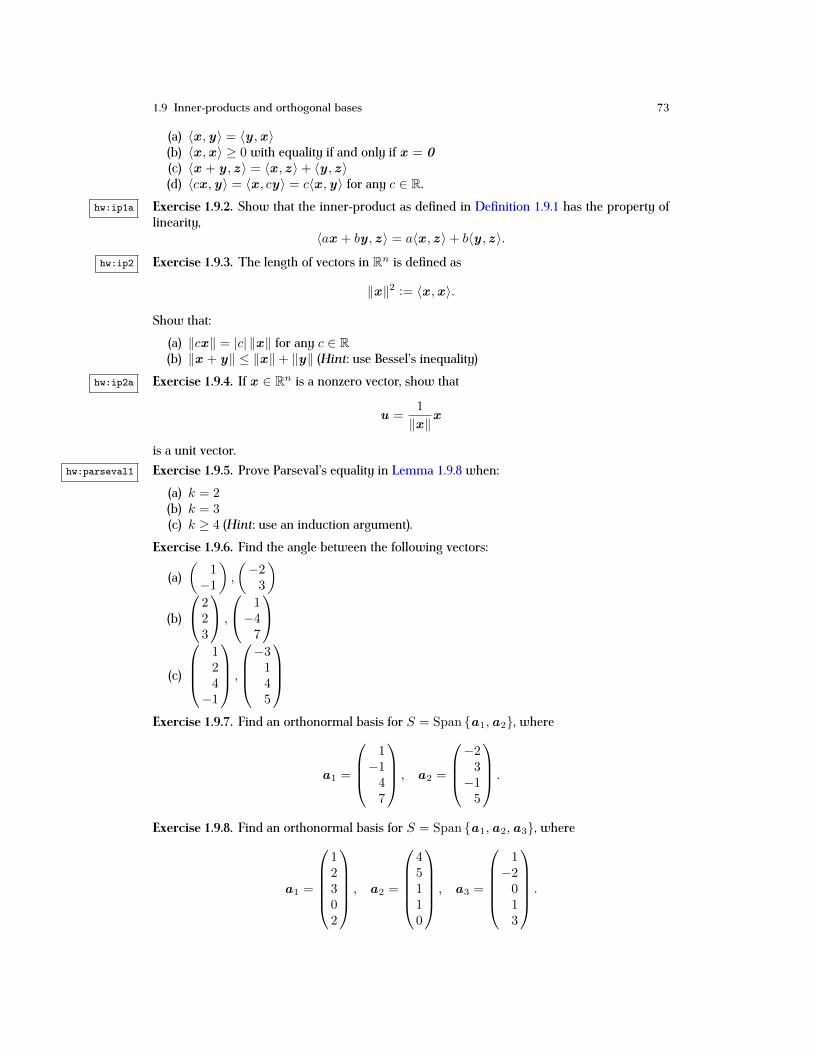
1.9 Inner-products and orthogonal bases 73
(a) 〈x ,y〉 = 〈y ,x 〉(b) 〈x ,x 〉 ≥ 0 with equality if and only if x = 0(c) 〈x + y , z 〉 = 〈x , z 〉+ 〈y , z 〉(d) 〈cx ,y〉 = 〈x , cy〉 = c〈x ,y〉 for any c ∈ R.
hw:ip1a Exercise 1.9.2. Show that the inner-product as defined in Definition 1.9.1 has the property oflinearity,
〈ax + by , z 〉 = a〈x , z 〉+ b〈y , z 〉.
hw:ip2 Exercise 1.9.3. The length of vectors in Rn is defined as
‖x‖2 := 〈x ,x 〉.
Show that:(a) ‖cx‖ = |c| ‖x‖ for any c ∈ R(b) ‖x + y‖ ≤ ‖x‖+ ‖y‖ (Hint: use Bessel’s inequality)
hw:ip2a Exercise 1.9.4. If x ∈ Rn is a nonzero vector, show that
u =1
‖x‖x
is a unit vector.hw:parseval1 Exercise 1.9.5. Prove Parseval’s equality in Lemma 1.9.8 when:
(a) k = 2(b) k = 3(c) k ≥ 4 (Hint: use an induction argument).
Exercise 1.9.6. Find the angle between the following vectors:
(a)(
1−1
),
(−23
)(b)
223
,
1−47
(c)
124−1
,
−3145
Exercise 1.9.7. Find an orthonormal basis for S = Span {a1,a2}, where
a1 =
1−147
, a2 =
−23−15
.
Exercise 1.9.8. Find an orthonormal basis for S = Span {a1,a2,a3}, where
a1 =
12302
, a2 =
45110
, a3 =
1−2013
.

74 1 Essentials of Linear Algebra
Exercise 1.9.9. Find an orthonormal basis for S = Span {a1,a2,a3}, where
a1 =
123
, a2 =
456
, a3 =
789
.
Exercise 1.9.10. Let
u1 =1√2
101
, u2 =1√6
12−1
, u3 =1√3
1−1−1
, b =
4−35
.
(a) Show that {u1,u2,u3} is an orthonormal basis for R3.(b) Find the Fourier coefficients associated with the vector b .(c) Find the Fourier expansion for the vector b in terms of the given basis vectors.(d) Use Parseval’s equality to find the length of b .
Exercise 1.9.11. Let
u1 =1√6
1012
, u2 =1√5
002−1
, u3 =1√31
−5112
, b =
7−17−1
.
(a) Show that {u1,u2,u3} is an orthonormal set of vectors.(b) Find the Fourier coefficients associated with the vector b .(c) Find the Fourier expansion for the vector b in terms of the given vectors.(d) Use Parseval’s equality to find the length of b .
hw:orthproj Exercise 1.9.12. Let {u1,u2, . . . ,uk} be an orthonormal set of vectors, and set
proj(x ) = 〈x ,u1〉u1 + 〈x ,u2〉u2 + · · ·+ 〈x ,uk〉uk.
The vector proj(x ) is known as the orthogonal projection of x onto the subspace S =Span{u1,u2, . . . ,uk}. Set r = x − proj(x ). The vector r is known as the residual. Showthat:
(a) 〈r , s〉 = 0 for any s ∈ S(b) proj[proj(x )] = proj(x )(c) if x ∈ S, then proj(x ) = x(d) if x ∈ S, then r = 0 .
hw:cper Exercise 1.9.13. Show that the space of continuous 2π-periodic functions, C0per, as defined in
(1.9.4) is a vector space under the definition given in Chapter 1.7.hw:cper2 Exercise 1.9.14. Show that the inner-product on the space C0
per defined by
〈f, g〉 =∫ 2π
0
f(x)g(x) dx
has the properties:
(a) 〈f, g〉 = 〈g, f〉(b) 〈f, f〉 ≥ 0 with equality if and only if f(x) ≡ 0(c) 〈f + g, h〉 = 〈f, h〉+ 〈g, h〉

1.10 The matrix transpose, and two more subspaces 75
(d) 〈cf, g〉 = 〈f, cg〉 = c〈f, g〉 for any c ∈ R.hw:cper3 Exercise 1.9.15. The length of a function in C0
per is defined by
‖f‖2 = 〈f, f〉.
Show that:(a) ‖cf‖ = |c| ‖f‖ for any c ∈ R(b) ‖f + g‖ ≤ ‖f‖+ ‖g‖ (the triangle inequality).
hw:cper4 Exercise 1.9.16. Consider the inner-product on the space C0per defined by
〈f, g〉 =∫ 2π
0
f(x)g(x) dx.
Show that for any integers j, k ≥ 1:
(a)⟨
1√2π,
1√2π
⟩= 1
(b)⟨
1√2π,
1√πcos(jx)
⟩= 0
(c)⟨
1√2π,
1√πsin(jx)
⟩= 0
(d)⟨
1√πcos(jx),
1√πcos(kx)
⟩=
{0, j 6= k
1, j = k
(e)⟨
1√πsin(jx),
1√πsin(kx)
⟩=
{0, j 6= k
1, j = k
(f)⟨
1√πsin(jx),
1√πcos(kx)
⟩= 0.
Exercise 1.9.17. Find Fourier expansions for the following products of trigonometric functionsusing the basis B3, which is defined in (1.9.5):
(a) sin(x) cos(2x)(b) sin(x) sin(2x)(c) cos(x) cos(2x)
Exercise 1.9.18. Find Fourier expansions for the following products of trigonometric functionsusing the basis B5, which is defined in (1.9.5):
(a) sin(x) sin(2x) cos(2x)(b) cos(x) sin(2x) cos(2x)(c) sin(x) cos(x) sin(3x)(d) cos(2x) cos(3x)(e) sin(2x) cos(3x)(f) sin(2x) sin(3x)
1.10 The matrix transpose, and two more subspaces
We now consider the transpose, AT, of matrix A. Writing A = (aij) ∈ Mm×n(R) for i =1, . . . ,m and j = 1, . . . , n, we have AT = (aji) ∈Mn×m(R). In other words, each column of

76 1 Essentials of Linear Algebra
A is a row of AT. For example,−132
T
= (−1 3 2) ⇔ (−1 3 2)T =
−132
,
and (−1 3 22 −5 8
)T
=
−1 23 −52 8
⇔
−1 23 −52 8
T
=
(−1 3 22 −5 8
).
The matrix transpose has the following properties (see Exercise 1.10.2):
(a) (AT)T = A(b) (cA)T = cAT for any constant c ∈ R(c) (A+B)T = AT +BT
(d) (AB)T = BTAT.
In our discussion of subspaces in Definition 1.5.1 and Definition 1.7.6 we considered twosubspaces associated with a matrix: the null space, and the column space. The matrix AT willalso have these two subspaces:
Null(AT) ={x : ATx = 0
}, Col(AT) =
{b : ATx = b is consistent
}.
In the above note that while Ax is a linear combination of the columns of A, ATx is a linearcombination of the rows of A. Since the columns of AT are the rows of A, the space Col(AT)is sometimes called the row space of A, and is the set of all linear combinations of the rows ofA. Moreover, since as a consequence of Exercise 1.10.2(d),
ATx = 0 (Ax )T= 0T xTA = 0T,
the null space of AT is sometimes called the left nullspace of A.
1.10.1 Subspace relationships
These four subspaces, Col(A), Null(A), Col(AT), Null(AT), are related both geometricallyand through dimension. First note that for A ∈Mm×n(R),
Col(A),Null(AT) ⊂ Rm, Null(A),Col(AT) ⊂ Rn.
Since they are subspaces of the same vector space, it is possible that there is some relationshipbetween Col(A) and Null(AT), and Col(AT) and Null(A). We have:
l:orthspace Lemma 1.10.1. If A ∈Mm×n(R), then
(a) b ∈ Col(A), x ∈ Null(AT) 〈b,x 〉 = 0(b) b ∈ Col(AT), x ∈ Null(A) 〈b,x 〉 = 0.

1.10 The matrix transpose, and two more subspaces 77
Proof. We will prove (a) only, and leave the proof of (b) for Exercise 1.10.10. The key to theproof is the result of Exercise 1.10.9,
〈Ax ,y〉 = 〈x ,ATy〉.
Since b ∈ Col(A), there is a vector x̃ such that Ax̃ = b . Since x ∈ Null(AT), ATx = 0 . Wethen have
〈b,x 〉 = 〈Ax̃ ,x 〉 = 〈x̃ ,ATx 〉 = 〈x̃ ,0 〉 = 0. ut
Using the definition of orthogonality provided in Definition 1.9.4, we see that vectors in thecolumn space of A are orthogonal to vectors in the null space of AT, and vectors in the columnspace of AT are orthogonal to vectors in the null space of A. All subspaces of a vector spaceshare the zero vector. We now show that is all the above subspaces share:
l:spaceint Corollary 1.10.2. If A ∈Mm×n(R), then
(a) Col(A) ∩Null(AT) = {0}(b) Null(A) ∩ Col(AT) = {0}.
Proof. We will prove (a) only, and leave the proof of (b) for Exercise 1.10.11. Suppose y ∈Col(A) ∩ Null(AT). By Lemma 1.10.1(a) we then have 〈y ,y〉 = 0. By definition of the innerproduct this is possible if and only if y = 0 . In other words, the only vector in both subspacesis the zero vector. ut
We conclude by observing that if a vector is orthogonal to every vector in the column spaceof A, then it must be a vector in the null space of AT.
thm:fredholm Lemma 1.10.3. Suppose A ∈ Mm×n(R). If 〈b,x 〉 = 0 for all b ∈ Col(A), thenx ∈ Null(AT).
Proof. Since b ∈ Col(A), there is a vector x̃ such that Ax̃ = b . We then have
0 = 〈b,x 〉 = 〈Ax̃ ,x 〉 = 〈x̃ ,ATx 〉.
The vector x̃ is arbitrary; consequently, the above calculation shows that the vector ATx ∈ Rnis orthogonal to any vector in Rn. Applying the result of Exercise 1.10.12 implies that ATx isthe zero vector, so ATx = 0 . In other words, x ∈ Null(AT). ut
We conclude by showing that even though Col(A) and Col(AT) are subspaces of differentvector spaces (assuming m 6= n), they are related through their dimension.
l:rank Lemma 1.10.4. If A ∈Mm×n(R), then
rank(A) = rank(AT).
Proof. Recall that:
(a) row reduction of a matrix is comprised of replacing rows with linear combinations ofrows; in particular, zero rows are formed by taking linear combinations of the rows
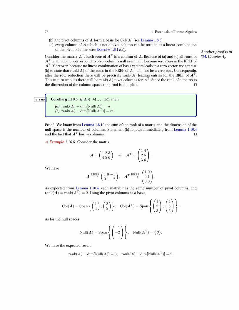
78 1 Essentials of Linear Algebra
(b) the pivot columns of A form a basis for Col(A) (see Lemma 1.8.3)(c) every column of A which is not a pivot column can be written as a linear combination
of the pivot columns (see Exercise 1.8.12(a)). Another proof is in[34, Chapter 4].Consider the matrix AT. Each row of AT is a column of A. Because of (a) and (c) all rows of
AT which do not correspond to pivot columns will eventually become zero rows in the RREF ofAT. Moreover, because no linear combination of basis vectors leads to a zero vector, we can use(b) to state that rank(A) of the rows in the RREF of AT will not be a zero row. Consequently,after the row reduction there will be precisely rank(A) leading entries for the RREF of AT.This in turn implies there will be rank(A) pivot columns for AT. Since the rank of a matrix isthe dimension of the column space, the proof is complete. ut
c:rank Corollary 1.10.5. If A ∈Mm×n(R), then
(a) rank(A) + dim[Null(A)] = n(b) rank(A) + dim[Null(AT)] = m.
Proof. We know from Lemma 1.8.10 the sum of the rank of a matrix and the dimension of thenull space is the number of columns. Statement (b) follows immediately from Lemma 1.10.4and the fact that AT has m columns. ut
C Example 1.10.6. Consider the matrix
A =
(1 2 34 5 6
) AT =
1 42 53 6
.
We have
ARREF−→
(1 0 −10 1 2
), AT RREF−→
1 00 10 0
.
As expected from Lemma 1.10.4, each matrix has the same number of pivot columns, andrank(A) = rank(AT) = 2. Using the pivot columns as a basis,
Col(A) = Span
{(14
),
(25
)}, Col(AT) = Span
1
23
,
456
.
As for the null spaces,
Null(A) = Span
1−21
, Null(AT) = {0}.
We have the expected result,
rank(A) + dim[Null(A)] = 3, rank(A) + dim[Null(AT)] = 2.

1.10 The matrix transpose, and two more subspaces 79
1.10.2 Least squares
The transpose of a coefficient matrix to can be used to “solve” an inconsistent linear system.Start with an overdetermined and inconsistent linear system,
Ax = b, A ∈Mm×n(R) (n ≤ m).
Such a system will arise, for example, in the context of data fitting. Suppose there are n points,(x1, y1), (x2, y2), . . . , (xn, yn), and further suppose that each point is thought to lie - but ac-tually does not - on a line of the form y = a1 + a2x for some constants a1 and a2. This impliesthe existence of a linear system,
a1 + a2x1 = y1
a1 + a2x2 = y2
...a1 + a2xn = yn,
which in matrix/vector form is
Aa = y ; A =
1 x11 x2...
...1 xn
, a =
(a1a2
), y =
y1y2...yn
.
As long as xj 6= xk for j 6= k, the matrix A will be of full rank, i.e., rank(A) = 2. It is clearthat this overdetermined system will in general be inconsistent, as it is too much to expect thateach data point lies on the same line.
AxAxLS
b
Ax−bAxLS−b
Col(A)
Fig. 1.4 (color online) A cartoon showing the relationship of the vector b with Col(A). Note the residualvectors Ax − b for arbitrary x , and AxLS − b for the least-squares solution xLS. f:LeastSquares
Going back to the original system, assume that the matrix has full rank, rank(A) = n. Forany x ∈ Rm we have Ax ∈ Col(A). Since the system is inconsistent, b /∈ Col(A). We wish to

80 1 Essentials of Linear Algebra
choose a vector, say xLS, such that the residual, AxLS − b , is as small as possible, i.e., for any The length of avector z ∈ Rn is‖z‖ =√z21 + · · ·+ z2n.
x ∈ Rm,‖AxLS − b‖ ≤ ‖Ax − b‖
(see Exercise 1.9.12 for another context in which a residual vector appears). Intuitively, thismeans the residual should be orthogonal to every vector in Col(A) (see Figure 1.4). As a conse-quence of Lemma 1.10.3) the residual must then be a vector in the null space of AT, AxLS−b ∈Null(AT) (also see Meyer [34, Chapter 5]). In other words,
AT (AxLS − b) = 0 ,
which can be rewritten (ATA
)xLS = ATb. (1.10.1) e:normaleq
The new linear system (1.10.1) is known as the normal equations. The coefficient matrixATA ∈Mn(R) is square. It turns out to be the case that A having full rank implies ATA hasfull rank (see Exercise 1.10.3). Consequently, the normal equations are consistent and have aunique solution (recall Theorem 1.8.13). These solutions are known as least-squares solutions.The least-squares solution, xLS, provides:
(a) the vector in Col(A), AxLS, which is closest to b(b) the solution to the original system, if the original system is consistent.
x
y
1
6
5
4
3
2
1
432
Fig. 1.5 (color online) The data points for Example 1.10.7, as well as a plot of the line of best fit,y = 3/2 + 11x/10. f:DataFit
ex:datafit C Example 1.10.7. Consider fitting a line to the data
(1, 2), (2, 4), (3, 6), (4, 5)
(see Figure 1.5). Writing y = a0 + a1x yields the system of inconsistent equations,

1.10 The matrix transpose, and two more subspaces 811 11 21 31 4
︸ ︷︷ ︸
A
a =
2465
︸ ︷︷ ︸b
, a =
(a0a1
).
It is clear that rank(A) = 2, so the matrix has full rank and the normal equations will have aunique solution. The normal equations are(
4 1010 30
)a = ATAa = ATb =
(1748
) a =
(3/2
11/10
).
The line of best fit isy =
3
2+
11
10x.
Exercises
Exercise 1.10.1. Let
A =
(1 −2 −5−2 3 −7
), B =
2 0−2 31 5
, C =
1 25 −43 −1
.
Compute the prescribed algebraic operation if it is well-defined. If it cannot be done, explainwhy.
(a) 2AT + 3B(b) A− 2CT
(c) CTA(d) BCT
(e) (BA)T
(f) (2A−BT)T
ex:182 Exercise 1.10.2. Let A,B ∈ Mm×n(R). Regarding properties of the transpose of a matrix,show that:
(a) (AT)T = A.(b) (cA)T = cAT for any constant c ∈ R.(c) (A+B)T = AT +BT.(d) (AB)T = BTAT.
hw:transpose Exercise 1.10.3. Suppose that A ∈Mm×n(R), n ≤ m, has full rank. Show that
rank(ATA) = rank(A) = n.
ex:183 Exercise 1.10.4. Suppose that A ∈Mn(R), and set
B = A+AT, C = A−AT.
(a) Show that B is symmetric, i.e., BT = B (hint: use Exercise 1.10.2).(b) Show that C is skew-symmetric, i.e., CT = −C (hint: use Exercise 1.10.2).
Exercise 1.10.5. Show that for any A ∈ Mm×n(R) the matrices AAT and ATA are bothsymmetric.

82 1 Essentials of Linear Algebra
Exercise 1.10.6. Show that if A is skew-symmetric, then all of its diagonal entries must be zero.Exercise 1.10.7. Show that any A ∈Mn(R) may be written as the sum of a symmetric matrixand a skew-symmetric matrix (hint: use Exercise 1.10.4).
hw:198inner Exercise 1.10.8. Show that the inner-product as defined in Definition 1.9.1 can also be writtenas
〈x ,y〉 = xTy .
hw:adj1 Exercise 1.10.9. Let A ∈ Mm×n(R). Show that 〈Ax ,y〉 = 〈x ,ATy〉. (Hint: Use Exer-cise 1.10.8 and the fact that (AB)T = BTAT.)
hw:adj2 Exercise 1.10.10. Let A ∈Mm×n(R). If b ∈ Col(AT) and x ∈ Null(A), show that 〈b,x 〉 = 0.(Hint: Use the definition of Col(A) and Exercise 1.10.9)
hw:adj3 Exercise 1.10.11. If A ∈Mm×n(R), show that Null(A) ∩ Col(AT) = {0}.hw:adj5 Exercise 1.10.12. Show that if 〈x ,y〉 = 0 for any vector y , then x = 0 . (Hint: consider the
particular case y = x )Exercise 1.10.13. Determine if each of the following statements is true or false. Provide anexplanation for your answer.
(a) If A,B ∈Mm×n(R) are the same size, then AB and BA are well-defined.(b) If A,B ∈M5(R), then AB = BA.(c) If A,B ∈Mn(R) are symmetric, then (AB)T = BA.(d) If A,B are such that A+B is well-defined, then (A+B)T = AT +BT.
Exercise 1.10.14. Find the line of best fit, y = a0 + a1x, for the data
(−1, 0), (0, 1), (1, 3), (2, 1), (3, 2).
Exercise 1.10.15. Find the quadratic of best fit, y = a0 + a1x+ a2x2, for the data
(−1, 0), (0, 1), (1, 3), (2, 1), (3, 2).
1.11 Matrix algebra: the inverse of a square matrixs:matinv
We learned how to do matrix addition/subtraction and multiplication in Chapter 1.3: how aboutmatrix division? If such a thing exists, then we can (formally) write the solution to linear systemsas
Ax = b x =1
Ab.
Unfortunately, as currently written this calculation makes no sense. However, using the analogythat 1/2 is the unique number such that 1/2 · 2 = 1, we could define 1/A to be that matrixsuch that 1/A ·A = I n. It is not clear that for a given matrix A the corresponding matrix 1/Amust exist. For an analogy, there is no number c ∈ R such that c · 0 = 1. Moreover, even if 1/Adoes exist, it is not at all clear as to how it should be computed.
When solving the linear system as above, we are implicitly assuming that
(a) a solution exists for any b(b) the solution is unique.
As we saw in Chapter 1.6.4, these two conditions can be satisfied only if the matrix is square.Consequently, for the rest of the discussion we will consider only square matrices, and we will
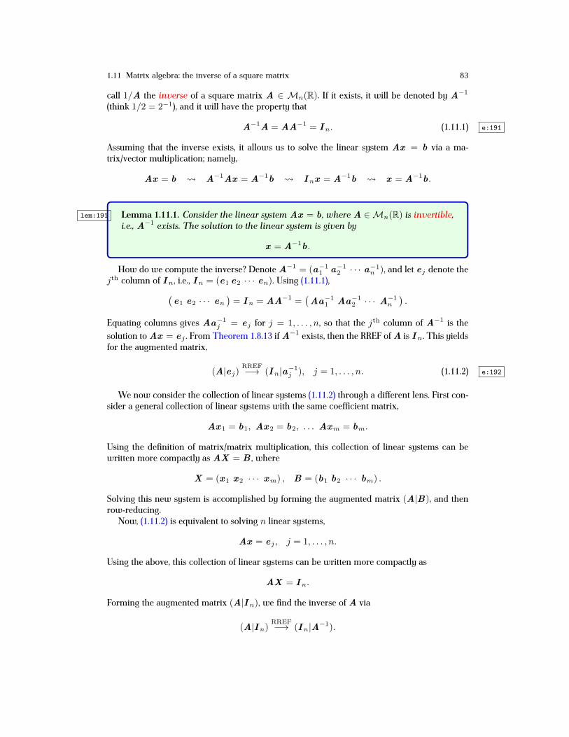
1.11 Matrix algebra: the inverse of a square matrix 83
call 1/A the inverse of a square matrix A ∈ Mn(R). If it exists, it will be denoted by A−1
(think 1/2 = 2−1), and it will have the property that
A−1A = AA−1 = I n. (1.11.1) e:191
Assuming that the inverse exists, it allows us to solve the linear system Ax = b via a ma-trix/vector multiplication; namely,
Ax = b A−1Ax = A−1b I nx = A−1b x = A−1b.
lem:191 Lemma 1.11.1. Consider the linear system Ax = b , where A ∈Mn(R) is invertible,i.e., A−1 exists. The solution to the linear system is given by
x = A−1b.
How do we compute the inverse? Denote A−1 = (a−11 a−12 · · · a−1n ), and let ej denote thejth column of I n, i.e., I n = (e1 e2 · · · en). Using (1.11.1),(
e1 e2 · · · en)= I n = AA−1 =
(Aa−11 Aa−12 · · · A−1n
).
Equating columns gives Aa−1j = ej for j = 1, . . . , n, so that the jth column of A−1 is thesolution to Ax = ej . From Theorem 1.8.13 if A−1 exists, then the RREF of A is I n. This yieldsfor the augmented matrix,
(A|ej)RREF−→ (I n|a−1j ), j = 1, . . . , n. (1.11.2) e:192
We now consider the collection of linear systems (1.11.2) through a different lens. First con-sider a general collection of linear systems with the same coefficient matrix,
Ax 1 = b1, Ax 2 = b2, . . . Axm = bm.
Using the definition of matrix/matrix multiplication, this collection of linear systems can bewritten more compactly as AX = B , where
X = (x 1 x 2 · · · xm) , B = (b1 b2 · · · bm) .
Solving this new system is accomplished by forming the augmented matrix (A|B), and thenrow-reducing.
Now, (1.11.2) is equivalent to solving n linear systems,
Ax = ej , j = 1, . . . , n.
Using the above, this collection of linear systems can be written more compactly as
AX = I n.
Forming the augmented matrix (A|I n), we find the inverse of A via
(A|I n)RREF−→ (I n|A−1).
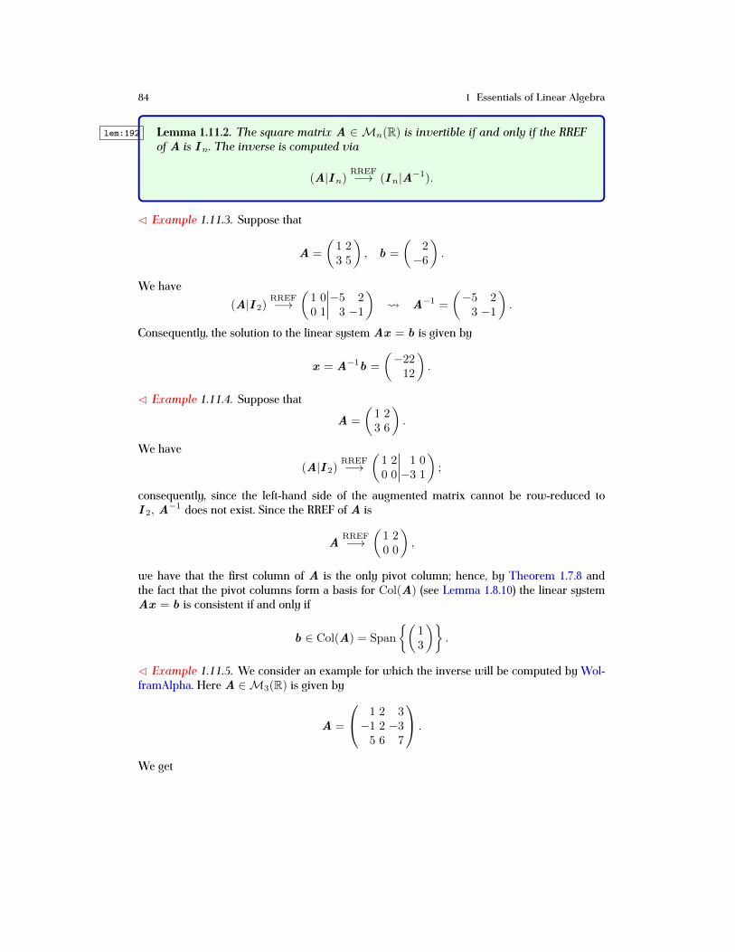
84 1 Essentials of Linear Algebra
lem:192 Lemma 1.11.2. The square matrix A ∈ Mn(R) is invertible if and only if the RREFof A is I n. The inverse is computed via
(A|I n)RREF−→ (I n|A−1).
C Example 1.11.3. Suppose that
A =
(1 23 5
), b =
(2−6
).
We have(A|I 2)
RREF−→(1 0 −5 20 1 3 −1
) A−1 =
(−5 23 −1
).
Consequently, the solution to the linear system Ax = b is given by
x = A−1b =
(−2212
).
C Example 1.11.4. Suppose that
A =
(1 23 6
).
We have(A|I 2)
RREF−→(1 2 1 00 0 −3 1
);
consequently, since the left-hand side of the augmented matrix cannot be row-reduced toI 2, A
−1 does not exist. Since the RREF of A is
ARREF−→
(1 20 0
),
we have that the first column of A is the only pivot column; hence, by Theorem 1.7.8 andthe fact that the pivot columns form a basis for Col(A) (see Lemma 1.8.10) the linear systemAx = b is consistent if and only if
b ∈ Col(A) = Span
{(13
)}.
C Example 1.11.5. We consider an example for which the inverse will be computed by Wol-framAlpha. Here A ∈M3(R) is given by
A =
1 2 3−1 2 −35 6 7
.
We get
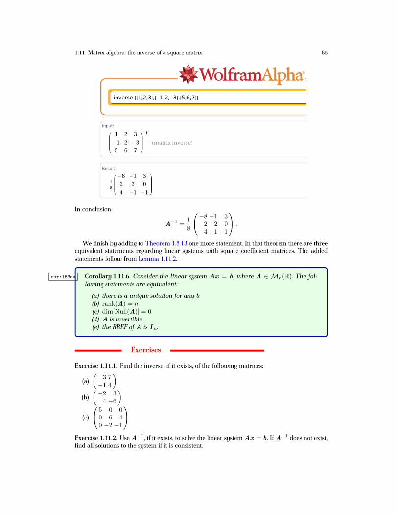
1.11 Matrix algebra: the inverse of a square matrix 85
inverse 881,2,3<,8-1,2,-3<,85,6,7<<
Input:
1 2 3
-1 2 -3
5 6 7
-1
Hmatrix inverseL
Result:
1
8
-8 -1 3
2 2 0
4 -1 -1
Dimensions:
3 HrowsL ´ 3 HcolumnsL
Matrix plot:
1 2 3
1
2
3
1 2 3
1
2
3
Determinant: Step-by-step solution
-1
32
Trace:
-7
8
Characteristic polynomial:
-x3
-7 x
2
8
+5 x
16
-1
32
Eigenvalues: Exact forms
Λ1 » -1.166
Λ2 » 0.145498 + 0.0750423 ä
Λ3 » 0.145498 - 0.0750423 ä
Generated by Wolfram|Alpha (www.wolframalpha.com) on March 27, 2014 from Champaign, IL.
© Wolfram Alpha LLC— A Wolfram Research Company1
In conclusion,
A−1 =1
8
−8 −1 32 2 04 −1 −1
.
We finish by adding to Theorem 1.8.13 one more statement. In that theorem there are threeequivalent statements regarding linear systems with square coefficient matrices. The addedstatements follow from Lemma 1.11.2.
cor:163aa Corollary 1.11.6. Consider the linear system Ax = b , where A ∈ Mn(R). The fol-lowing statements are equivalent:
(a) there is a unique solution for any b(b) rank(A) = n(c) dim[Null(A)] = 0(d) A is invertible(e) the RREF of A is I n.
Exercises
Exercise 1.11.1. Find the inverse, if it exists, of the following matrices:
(a)(
3 7−1 4
)(b)(−2 34 −6
)(c)
5 0 00 6 40 −2 −1
Exercise 1.11.2. Use A−1, if it exists, to solve the linear system Ax = b . If A−1 does not exist,find all solutions to the system if it is consistent.
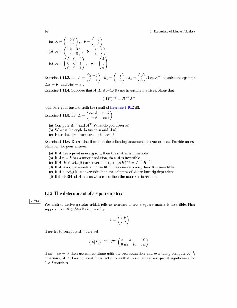
86 1 Essentials of Linear Algebra
(a) A =
(3 7−1 4
), b =
(5−6
)(b) A =
(−2 34 −6
), b =
(−48
)(c) A =
5 0 00 6 40 −2 −1
, b =
319
Exercise 1.11.3. Let A =
(2 −53 4
), b1 =
(7−8
), b2 =
(06
). Use A−1 to solve the systems
Ax = b1 and Ax = b2.Exercise 1.11.4. Suppose that A,B ∈Mn(R) are invertible matrices. Show that
(AB)−1 = B−1A−1
(compare your answer with the result of Exercise 1.10.2(d)).
Exercise 1.11.5. Let A =
(cos θ − sin θsin θ cos θ
).
(a) Compute A−1 and AT. What do you observe?(b) What is the angle between v and Av?(c) How does ‖v‖ compare with ‖Av‖?
Exercise 1.11.6. Determine if each of the following statements is true or false. Provide an ex-planation for your answer.
(a) If A has a pivot in every row, then the matrix is invertible.(b) If Ax = b has a unique solution, then A is invertible.(c) If A,B ∈Mn(R) are invertible, then (AB)−1 = A−1B−1.(d) If A is a square matrix whose RREF has one zero row, then A is invertible.(e) If A ∈Mn(R) is invertible, then the columns of A are linearly dependent.(f) If the RREF of A has no zero rows, then the matrix is invertible.
1.12 The determinant of a square matrixs:210
We wish to derive a scalar which tells us whether or not a square matrix is invertible. Firstsuppose that A ∈M2(R) is given by
A =
(a bc d
).
If we try to compute A−1, we get
(A|I 2)−cρ1+aρ2−→
(a b 1 00 ad− bc −c a
).
If ad − bc 6= 0, then we can continue with the row reduction, and eventually compute A−1;otherwise, A−1 does not exist. This fact implies that this quantity has special significance for2× 2 matrices.
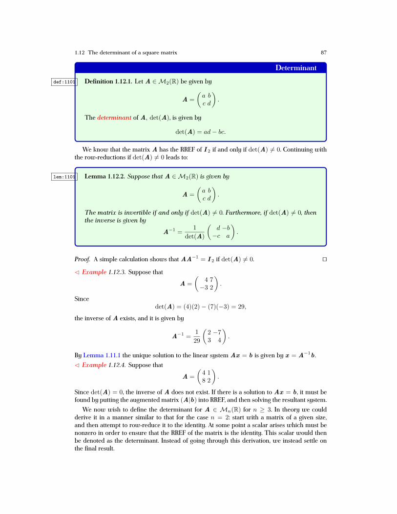
1.12 The determinant of a square matrix 87
Determinantdef:1101 Definition 1.12.1. Let A ∈M2(R) be given by
A =
(a bc d
).
The determinant of A, det(A), is given by
det(A) = ad− bc.
We know that the matrix A has the RREF of I 2 if and only if det(A) 6= 0. Continuing withthe row-reductions if det(A) 6= 0 leads to:
lem:1101 Lemma 1.12.2. Suppose that A ∈M2(R) is given by
A =
(a bc d
).
The matrix is invertible if and only if det(A) 6= 0. Furthermore, if det(A) 6= 0, thenthe inverse is given by
A−1 =1
det(A)
(d −b−c a
).
Proof. A simple calculation shows that AA−1 = I 2 if det(A) 6= 0. ut
C Example 1.12.3. Suppose that
A =
(4 7−3 2
).
Sincedet(A) = (4)(2)− (7)(−3) = 29,
the inverse of A exists, and it is given by
A−1 =1
29
(2 −73 4
).
By Lemma 1.11.1 the unique solution to the linear system Ax = b is given by x = A−1b .C Example 1.12.4. Suppose that
A =
(4 18 2
).
Since det(A) = 0, the inverse of A does not exist. If there is a solution to Ax = b , it must befound by putting the augmented matrix (A|b) into RREF, and then solving the resultant system.
We now wish to define the determinant for A ∈ Mn(R) for n ≥ 3. In theory we couldderive it in a manner similar to that for the case n = 2: start with a matrix of a given size,and then attempt to row-reduce it to the identity. At some point a scalar arises which must benonzero in order to ensure that the RREF of the matrix is the identity. This scalar would thenbe denoted as the determinant. Instead of going through this derivation, we instead settle onthe final result.

88 1 Essentials of Linear Algebra
For A ∈ Mn(R), let Aij ∈ Mn−1(R) denote the submatrix gotten from A after deletingthe ith row and jth column. For example,
A =
1 4 72 5 83 6 9
=⇒ A12 =
(2 83 9
), A31 =
(4 75 8
).
With this notion of submatrix in mind, we note that for 2× 2 matrices the determinant can bewritten as
det(A) = a11 det(A11)− a12 det(A12),
where here the determinant of a scalar is simply the scalar. The generalization to larger matricesis:
Determinantdef:1102 Definition 1.12.5. If A ∈Mn(R), then the determinant of A is given by
det(A) = a11 det(A11)− a12 det(A12) + a13 det(A13) + · · ·+ (−1)n+1a1n det(A1n).
C Example 1.12.6. If
A =
1 4 72 5 83 6 9
,
then we haveA11 =
(5 86 9
), A12 =
(2 83 9
), A13 =
(2 53 6
).
Sincea11 = 1, a12 = 4, a13 = 7,
the determinant of the matrix is
det(A) = 1 · det(A11)− 4 · det(A12) + 7 · det(A13) = −3 + 24− 21 = 0.
Thus, we know that A−1 does not exist; indeed, the RREF of A is
ARREF−→
1 0 −10 1 20 0 0
,
and the columns of A are linearly dependent. Indeed,
Col(A) = Span
1
23
,
456
, Null(A) = Span
1−21
,
with rank(A) = 2 and dim[Null(A)] = 1. The columns are related through the linear combi-nation a1 − 2a2 + a3 = 0 .C Example 1.12.7. We now calculate the determinant using WolframAlpha for the matrix

1.12 The determinant of a square matrix 89
A =
1 2 3−1 2 −35 6 7
.
We have
det 881,2,3<,8-1,2,-3<,85,6,7<<
Input interpretation:
1 2 3
-1 2 -3
5 6 7
m¤ is the determinant»
Result: Step-by-step solution
-32
Number name:
negative thirty-two
Number line:
-60 -50 -40 -30 -20 -10
Generated by Wolfram|Alpha (www.wolframalpha.com) on March 27, 2014 from Champaign, IL.
© Wolfram Alpha LLC— A Wolfram Research Company1
In other words, det(A) = −32.The determinant has many properties, which are too many to detail in full here (e.g., see
Eves [18, Chapter 3] and Vein and Dale [41]). We will consider only a small number that we willdirectly need. The first, and perhaps most important, is that the expression of Definition 1.12.1is not the only way to calculate the determinant. In general, the determinant can be calculatedby going across any row, or down any column; in particular, we have
det(A) =
n∑j=1
(−1)i+jaij det(Aij)︸ ︷︷ ︸across ith row
=
n∑i=1
(−1)i+jaij det(Aij)︸ ︷︷ ︸down jth column
. (1.12.1) e:1101
For example,
det
4 3 62 0 0−1 7 −5
= (6) det
(2 0−1 7
)− (0) det
(4 3−1 7
)+ (−5) det
(4 32 0
)
= −(2) det(3 67 −5
)+ (0) det
(4 6−1 −5
)− (0) det
(4 3−1 7
).
The first line is down the third column, and the second line is across the second row. As theabove example shows, a judicious choice for the expansion of the determinant can greatlysimplify the calculation. In particular, it is generally best to calculate the determinant using therow or column which has the most zeros. Note that if a matrix has a zero row or column, thenby using the more general definition (1.12.1) and expanding across that zero row or column weget that det(A) = 0.
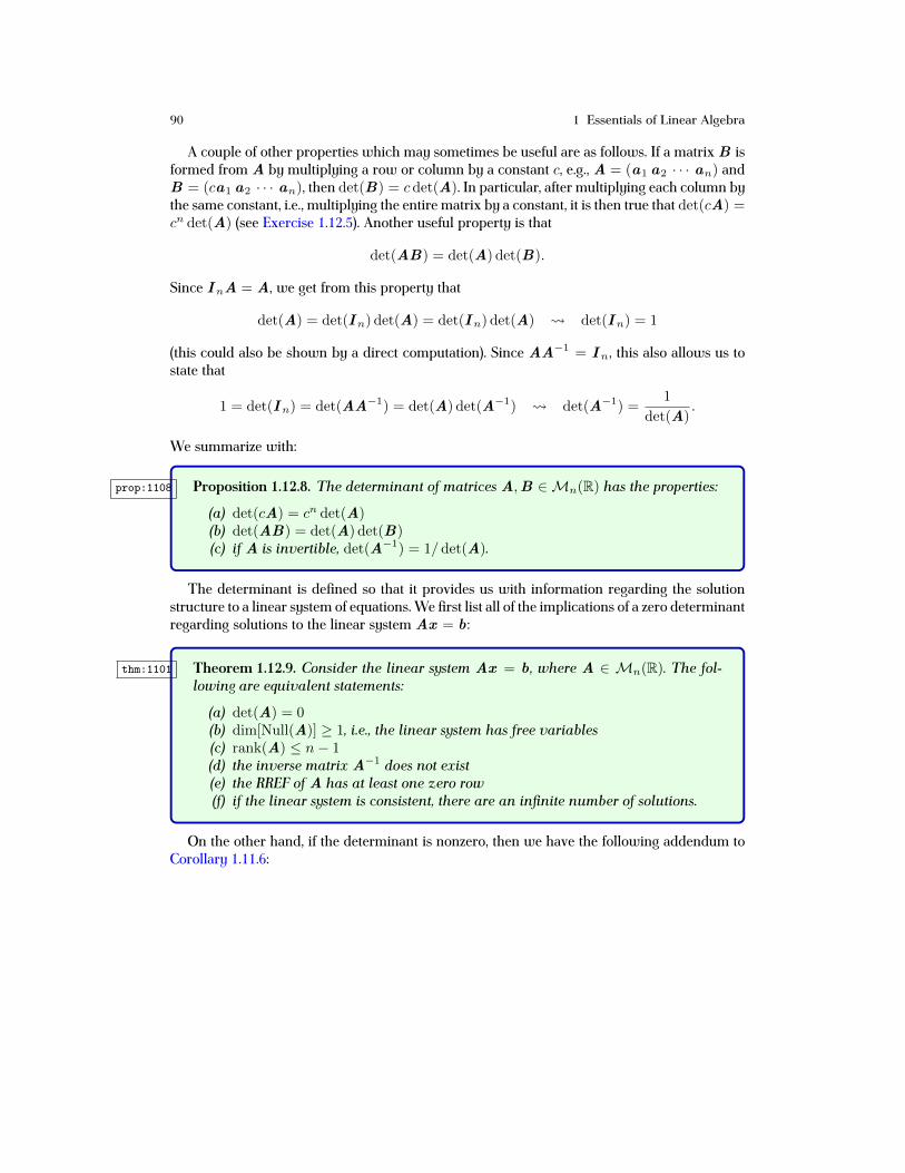
90 1 Essentials of Linear Algebra
A couple of other properties which may sometimes be useful are as follows. If a matrix B isformed from A by multiplying a row or column by a constant c, e.g., A = (a1 a2 · · · an) andB = (ca1 a2 · · · an), then det(B) = cdet(A). In particular, after multiplying each column bythe same constant, i.e., multiplying the entire matrix by a constant, it is then true that det(cA) =cn det(A) (see Exercise 1.12.5). Another useful property is that
det(AB) = det(A) det(B).
Since I nA = A, we get from this property that
det(A) = det(I n) det(A) = det(I n) det(A) det(I n) = 1
(this could also be shown by a direct computation). Since AA−1 = I n, this also allows us tostate that
1 = det(I n) = det(AA−1) = det(A) det(A−1) det(A−1) =1
det(A).
We summarize with:
prop:1108 Proposition 1.12.8. The determinant of matrices A,B ∈Mn(R) has the properties:
(a) det(cA) = cn det(A)(b) det(AB) = det(A) det(B)(c) if A is invertible, det(A−1) = 1/ det(A).
The determinant is defined so that it provides us with information regarding the solutionstructure to a linear system of equations. We first list all of the implications of a zero determinantregarding solutions to the linear system Ax = b :
thm:1101 Theorem 1.12.9. Consider the linear system Ax = b , where A ∈ Mn(R). The fol-lowing are equivalent statements:
(a) det(A) = 0(b) dim[Null(A)] ≥ 1, i.e., the linear system has free variables(c) rank(A) ≤ n− 1(d) the inverse matrix A−1 does not exist(e) the RREF of A has at least one zero row(f) if the linear system is consistent, there are an infinite number of solutions.
On the other hand, if the determinant is nonzero, then we have the following addendum toCorollary 1.11.6:
1.12 The determinant of a square matrix 91
thm:1101aa Theorem 1.12.10. Consider the linear system Ax = b , where A ∈ Mn(R). Thefollowing are equivalent:
(g) det(A) 6= 0(h) dim[Null(A)] = 0(i) rank(A) = n, i.e., A has full rank(j) the inverse matrix A−1 exists
(k) the RREF of A is the identity matrix I n(l) the linear system is consistent, and the unique solution is x = A−1b .
Exercises
Exercise 1.12.1. Compute by hand det(A) for each of the following matrices, and then statewhether or not the matrix is invertible. If the matrix is invertible, compute det(A−1).
(a) A =
(3 −2−2 3
)(b) A =
1 −3 41 2 −13 −5 8
(c) A =
1 2 30 4 02 8 5
(d) A =
1 2 0 52 4 0 60 −3 0 56 −1 2 4
ex:1103 Exercise 1.12.2. Suppose that A ∈Mn(R).
(a) If n = 2, show that det(AT) = det(A).(b) If n = 3, show that det(AT) = det(A).(c) Show that det(AT) = det(A) for any n.
Exercise 1.12.3. Suppose that A,B ∈Mn(R). Show that the matrix product AB is invertibleif and only if both A and B are invertible. (Hint: Use Proposition 1.12.8(b))
hw:diagdet Exercise 1.12.4. Suppose that D = diag(λ1, λ2, . . . , λn) is a diagonal matrix, e.g.,
diag(λ1, λ2) =
(λ1 00 λ2
), diag(λ1, λ2, λ3) =
λ1 0 00 λ2 00 0 λ3
, etc.
(a) If n = 2, show that det(D) = λ1λ2.(b) If n = 3, show that det(D) = λ1λ2λ3.(c) Show that for any n,
det(D) =
n∏j=1
λj .
hw:2102 Exercise 1.12.5. Here we generalize the result of Proposition 1.12.8(a). For a matrix A =(a1 a2 a3 · · · an) ∈Mn(R), let B be defined as B = (c1a1 c2a2 c3a3 · · · cnan).

92 1 Essentials of Linear Algebra
(a) Show that B = AC , where C = diag(c1, c2, . . . , cn) is a diagonal matrix.(b) If n = 2, show that det(B) = c1c2 det(A).(c) Show that for n ≥ 3,
det(B) =
n∏j=1
cj
det(A).
(Hint: Use Proposition 1.12.8(b) and Exercise 1.12.4)Exercise 1.12.6. Suppose that A ∈Mn(R) is an upper triangular matrix, i.e., all of the entriesbelow the diagonal are zero.
(a) Show that det(A) is the product of the diagonal entries. Hint: Show that it is true forn = 2, 3, and then use an induction argument.
(b) Show that AT is a lower triangular matrix, i.e., all of the entries above the diagonal arezero.
(c) Show that det(AT) is the product of the diagonal entries. Hint: Use the result of Exer-cise 1.12.2.
Exercise 1.12.7. A matrix V ∈M3(R) is said to be a Vandermonde matrix if
V =
1 a a2
1 b b2
1 c c2
.
(a) Show that det(V ) = (b− a)(c− a)(c− b).(b) What conditions must the scalars a, b, c satisfy in order that V be invertible?
Exercise 1.12.8. Suppose that
A(λ) =
(3− λ −2−2 3− λ
).
For which value(s) of λ does the system A(λ)x = 0 have a nontrivial solution? For one suchvalue of λ, compute a corresponding nontrivial solution.Exercise 1.12.9. Suppose that A ∈Mn(R) is such that Ax = 0 has infinitely many solutions.What can be said about det(A)? Explain.Exercise 1.12.10. Determine if each of the following statements is true or false. Provide anexplanation for your answer.
(a) If A ∈Mn(R) has a pivot in every row, then det(A) = 0.(b) If A ∈Mn(R) and Ax = b has a unique solution for any b , then det(A) = 0.(c) If A ∈Mn(R) is a diagonal matrix, then det(A) is the product of the diagonal entries.(d) If the RREF of A ∈Mn(R) has one zero row, then det(A) 6= 0.
1.13 Linear algebra with complex-valued numbers, vectors, and matricess:complexnum
Before we proceed to our last topic on matrices, we will need to understand the basics associatedwith complex-valued numbers, and the associated algebraic manipulations. As we will see, thesewill be naturally encountered in future calculations with square matrices, even if the matrix inquestion contains only real-valued entries.
We say that z ∈ C if z = a+ib, where a, b ∈ R, and i2 = −1. The number a is the real partof the complex number, and is sometimes denoted by Re(z), i.e., Re(z) = a. The number b is

1.13 Linear algebra with complex-valued numbers, vectors, and matrices 93
the imaginary part of the complex number, and is sometimes denoted by Im(z), i.e., Im(z) = b.We say a vector v ∈ Cn if each entry is complex-valued, and we will often write
v = p + iq , p, q ∈ Rn.
The vector p is the real part of v , i.e., Re(v) = p , and the vector q is the imaginary part, i.e.,Im(v) = q . For example,(
1− i52 + i7
)=
(12
)+ i
(−57
) p =
(12
), q =
(−57
).
We say that a matrix A ∈Mm×n(C) if each entry of the matrix is (possibly) complex-valued.The addition/subtraction of two complex numbers is as expected: add/subtract the real parts
and imaginary parts. For example,
(2− i3) + (3 + i2) = (2 + 3) + i(−3 + 2) = 5− i.
As for multiplication, we multiply products of sums in the usual way, and use the fact thati2 = −1; for example,
(2− i3)(3 + i2) = (2)(3) + (−i3)(3) + (2)(i2) + (−i3)(i2)= 6− i9 + i4− i26 = 12− i5.
In particular, note thatc(a+ ib) = ac+ ibc,
i.e., multiplication of a complex number by a real number gives a complex number in whichthe real and imaginary parts of the original number are both multiplied by the real number.For example,
7(−4 + i9) = −28 + i63.
Before we can consider the problem of division, we must first think about the size of acomplex number. The complex-conjugate of a complex number z, which is denoted by z, isgiven by taking the negative of the imaginary part, i.e.,
z = a+ ib z = a− ib.
If the number is real-valued, then z = z. The complex-conjugate of a a vector v ∈ Cn is givenby
v = p + iq = p − iq .
The complex-conjugate of a matrix A is written as A, and the definition is what is to be ex-pected. If A = (ajk), then A = (ajk). For example,
A =
(2− i5 31 + i7 −3 + i5
) A =
(2 + i5 31− i7 −3− i5
).
Regarding the conjugate, it is not difficult to check that
z1z2 = z1 z2,
i.e., the conjugate of a product is the product of the conjugates (see Exercise 1.13.1(a)). We furtherhave

94 1 Essentials of Linear Algebra
zz = (a+ ib)(a− ib) = a2 + b2 > 0,
and using this fact we say that the magnitude (absolute value) of a complex number is
|z| =√zz =
√a2 + b2.
It is not difficult to check that|z1z2| = |z1| |z2|,
i.e., the magnitude of a product is the product of the magnitudes (see Exercise 1.13.1(b)).We consider the division of two complex numbers by thinking of it as a multiplication prob-
lem. We first multiply the complex number by the number one represented as the complex-conjugate of the denominator divided by the complex-conjugate of the denominator. We thenwrite
z1z2
=z1z2
z2z2
=1
z2z2z1z2 =
1
|z2|2z1z2,
so that division has been replaced by the appropriate multiplication. For example,
2− i3
3 + i2=
(2− i3
3 + i2
)(3− i2
3− i2
)=
1
13[(2− i3)(3− i2)] =
1
13(−i13) = −i.
We now derive and state a very important identity - Euler’s formula - which connects the ex-ponential function to the sine and cosine. This will be accomplished via the use of the Maclaurinseries for the exponential and trigonometric functions. Recall that
ex =
∞∑j=0
xj
j!= 1 + x+
x2
2!+x3
3!+ · · ·
sin(x) =
∞∑j=0
(−1)j x2j+1
(2j + 1)!= x− x3
3!+x5
5!− x7
7!+ · · ·
cos(x) =
∞∑j=0
(−1)j x2j
(2j)!= 1− x2
2!+x4
4!− x6
6!+ · · · ,
and that each series converges for all x ∈ R. Since
i2 = −1, i3 = i2i = −i, i4 = i2i2 = 1,
we can write for θ ∈ R,
eiθ =
∞∑j=0
(iθ)j
j!= 1 + iθ − θ2
2!− i
θ3
3!+θ4
4!+ i
θ5
5!+ · · ·
=
(1− θ2
2!+θ4
4!+ · · ·+ (−1)j θ
2j
(2j)!+ · · ·
)+
i
(θ − θ3
3!+θ5
5!+ · · ·+ (−1)j θ2j+1
(2j + 1)!+ · · ·
).
Noting that the real part is the Maclaurin series for cos(θ), and the imaginary part is the Maclau-rin series for sin(θ), we arrive at Euler’s formula,
eiθ = cos(θ) + i sin(θ).
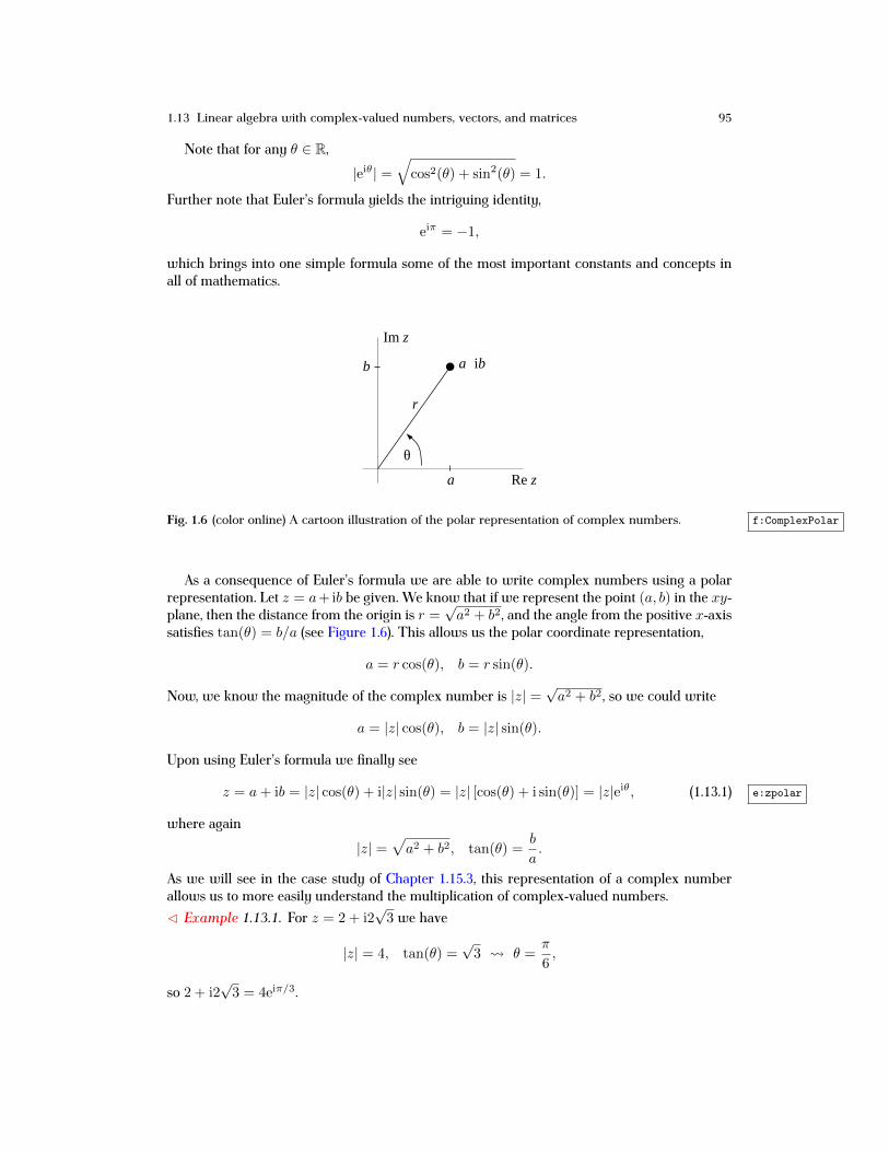
1.13 Linear algebra with complex-valued numbers, vectors, and matrices 95
Note that for any θ ∈ R,|eiθ| =
√cos2(θ) + sin2(θ) = 1.
Further note that Euler’s formula yields the intriguing identity,
eiπ = −1,
which brings into one simple formula some of the most important constants and concepts inall of mathematics.
a
b
Re z
Im z
θ
r
a+ib
Fig. 1.6 (color online) A cartoon illustration of the polar representation of complex numbers. f:ComplexPolar
As a consequence of Euler’s formula we are able to write complex numbers using a polarrepresentation. Let z = a+ib be given. We know that if we represent the point (a, b) in the xy-plane, then the distance from the origin is r =
√a2 + b2, and the angle from the positive x-axis
satisfies tan(θ) = b/a (see Figure 1.6). This allows us the polar coordinate representation,
a = r cos(θ), b = r sin(θ).
Now, we know the magnitude of the complex number is |z| =√a2 + b2, so we could write
a = |z| cos(θ), b = |z| sin(θ).
Upon using Euler’s formula we finally see
z = a+ ib = |z| cos(θ) + i|z| sin(θ) = |z| [cos(θ) + i sin(θ)] = |z|eiθ, (1.13.1) e:zpolar
where again
|z| =√a2 + b2, tan(θ) =
b
a.
As we will see in the case study of Chapter 1.15.3, this representation of a complex numberallows us to more easily understand the multiplication of complex-valued numbers.C Example 1.13.1. For z = 2 + i2
√3 we have
|z| = 4, tan(θ) =√3 θ =
π
6,
so 2 + i2√3 = 4eiπ/3.

96 1 Essentials of Linear Algebra
C Example 1.13.2. For z = −2√3 + i2 we have
|z| = 4, tan(θ) = − 1√3 θ =
5π
6.
The choice for the angle follows from the fact that the point (−2√3, 2) is in the second quadrant
of the xy-plane. In conclusion, −2√3 + i2 = 4ei5π/6.
Does anything really change if we consider the previous linear algebra calculationsand concepts under the assumption that the matrices and vectors have complex-valuedentries? In summary, no. The definitions and properties of the span of a set of vectors,and subspaces - in particular, the subspaces Null(A) and Col(A) - remain the same;indeed, the only difference is that the constants may now be complex-valued. A basisof a subspace is still computed in the same manner, and the dimension of a subspace isstill the number of basis vectors. Again, the only difference is that the vectors may havecomplex-valued entries. As for the inner-product, if we define it for vectors on Cn as
〈x ,y〉 =n∑j=1
xjyj = x1y1 + x2y2 + · · ·+ xnyn,
then the desired properties will still hold. In particular, we will still have 〈x ,x 〉 is anonnegative real number, and will be zero if and only if x = 0 . Finally, nothing changesfor matrix/vector and matrix/matrix multiplication, the calculation of the inverse of asquare matrix, and the calculation of the determinant for a square matrix. In conclusion,the only reason we did not start the chapter with a discussion of linear systems withcomplex-valued coefficients is for the sake of pedagogy, as it is easier to visualize vectorsin Rn, and subspaces which are realized as real-valued linear combinations of vectorsin Rn.
C Example 1.13.3. Let us see how we can use our understanding of the algebra of complexnumbers when doing Gaussian elimination. Consider the linear system
(1− i)x1 + 4x2 = 6
(−2 + i3)x1 + (−8 + i3)x2 = −9.
Performing Gaussian elimination on the augmented matrix yields(1− i 4 6
−2 + i3 −8 + i3 −9
)(1/(1−i))ρ1−→
(1 2 + i2 3 + i3
−2 + i3 −8 + i3 −9
)(2−i3)ρ1+ρ2−→
(1 2 + i2 3 + i30 −2 + i 6− i3
)(1/(−2+i))ρ2−→
(1 2 + i2 3 + i30 1 −3
)(−2−i2)ρ2+ρ1−→
(1 0 9 + i90 1 −3
).
The solution is the last column,
x =
(9 + i9−3
)= x =
(9−3
)+ ix =
(90
).

1.13 Linear algebra with complex-valued numbers, vectors, and matrices 97
C Example 1.13.4. For another example, let us find Null(A) for the matrix
A =
(3− i 45 6 + i2
).
SinceA
RREF−→(1 (6 + i2)/50 0
),
the null space is found by solving
x1 +6 + i2
5x2 = 0.
Upon setting x2 = 5t the solution vector is given by
x =
(−(6 + i2)t
5t
)= t
(−6− i2
5
).
We conclude that
Null(A) = Span
{(−6− i2
5
)}, dim[Null(A)] = 1.
C Example 1.13.5. Let us find those vectors b for which the linear system Ax = b is consistentwith
A =
(2− i 45 8 + i4
).
Gaussian elimination yields that the RREF of A is
ARREF−→
(1 (8 + i4)/50 0
).
Since the RREF of A has a zero row, the system Ax = b is not consistent for all b . Moreover,only the first column is a pivot column, so by using Lemma 1.8.10 we know that a basis forCol(A) is the first column of A, i.e.,
Col(A) = Span
{(2− i5
)}, rank(A) = 1.
The linear system is consistent if and only if b ∈ Col(A).
Exercises
hw:complexconj Exercise 1.13.1. Let z1 = a1 + ib1 and z2 = a2 + ib2 be two complex numbers. Show that
(a) z1z2 = z1 z2(b) |z1z2| = |z1| |z2|.
Exercise 1.13.2. Write each complex number z in the form |z|eiθ , where −π < θ ≤ π.
(a) z = 3− i4(b) z = −2 + i5(c) z = −3− i7(d) z = 6 + i

98 1 Essentials of Linear Algebra
Exercise 1.13.3. Solve each system of equations, or explain why no solution exists.
(a) (3− i)x1 + 2x2 = 2, −4x1 + (1 + i4)x2 = −3(b) x1 + (−2 + i5)x2 = −3, (1− i5)x1 + 3x2 = 12
Exercise 1.13.4. For each of the below problems compute the product Ax when it is well-defined. If the product cannot be computed, explain why.
(a) A =
2 + i 3−2 1 + i43 7
, x =
(2 + i3
8
)
(b) A =
(2 −1 + i3 −4
2 + i5 6 3− i7
), x =
29
4 + i3
.
Exercise 1.13.5. For each matrix A, find Null(A), and determine its dimension.
(a) A =
(2 + i3 262 8− i12
)(b) A =
(1− i4 172 2 + i8
)Exercise 1.13.6. Solve the following linear system, and explicitly identify the homogeneoussolution, xh, and the particular solution, xp:(
3 + i2 −26−2 12− i8
)x =
(13
−6 + i4
).
hw:2125 Exercise 1.13.7. In Example 1.8.8 it was shown that dim[Rn] = n. Show that dim[Cn] = n.
1.14 Eigenvalues and eigenvectorss:2112
Consider a square matrix A ∈ Mn(R). As we will see in the two case studies in Chapter 1.15,as well as when solving homogeneous systems of ODEs in ??, it will be especially useful toidentify a set of vectors, say v1, v2, . . . , vn, such that for each vector there is a constant λj suchthat
Av j = λjv j , j = 1, . . . , n. (1.14.1) e:2112aa
The vectors v j , which are known as eigenvectors, and multiplicative factors λj , which areknown as eigenvalues, may be complex-valued (see Chapter 1.13). If the eigenvalues arecomplex-valued, then the corresponding eigenvector also has complex-valued entries. Eigen-vectors are vectors that have the property that matrix multiplication by A leads to a scalarmultiple of the original vector.
1.14.1 Characterization of eigenvalues and eigenvectors
How do we find these vectors v and associated multiplicative factors λ? We can rewrite 1.14.1as
Av = λv (A− λI n)v = 0 .

1.14 Eigenvalues and eigenvectors 99
Recalling the definition of a null space, an eigenvector v can be found if we can find an eigen-value λ such that
dim[Null(A− λI n)] ≥ 1.
If λ is an eigenvalue, then we will call Null(A − λI n) the eigenspace. An eigenvector is anybasis vector of the eigenspace.
Eigenvectors associated with a particular eigenvalue are not unique, as a basis is notunique (recall the discussion in Chapter 1.8). However, the number of basis vectors isunique (recall Lemma 1.8.6), so associated with each eigenvalue there will be a fixednumber of linearly independent eigenvectors.
Now, if we are given an eigenvalue, then it is straightforward to compute a basis for the as-sociated eigenspace. The problem really is in finding an eigenvalue. This requires an additionalequation, for at the moment the linear system is a set of n equations with n+1 variables: the ncomponents of the vector plus the associated eigenvalue. In constructing this additional equa-tion we can rely upon the result of Theorem 1.12.9, in which it is stated that a square matrixhas a nontrivial null space if and only if its determinant is zero. If we set
pA(λ) = det(A− λI n),
then the eigenvalues will correspond to the zeros of the characteristic polynomial pA(λ). Whilewe will not do it here, it is not difficult to show that the characteristic polynomial is a polynomialof degree n, the size of the square matrix (see Exercise 1.14.4).
We summarize this discussion with the following result:
thm:1111 Theorem 1.14.1. Let A ∈ Mn(R). The zeros of the nth-order characteristic polyno-mial pA(λ) = det(A − λI n) are the eigenvalues of the matrix A. The (not unique)eigenvectors associated with an eigenvalue are a basis for Null(A− λI n).
Before going any further in the discussion of the theory associated with eigenvalues andeigenvectors, let us do a relatively simple computation.C Example 1.14.2. Let us find the eigenvalues and associated eigenvectors for
A =
(3 22 3
).
We haveA− λI 2 =
(3− λ 22 3− λ
),
so that the characteristic polynomial is
pA(λ) = (3− λ)2 − 4.
The zeros of the characteristic polynomial are λ = 1, 5. As for the associated eigenvectors, wemust compute a basis for Null(A − λI 2) for each eigenvalue. For the eigenvalue λ1 = 1 wehave
A− I 2RREF−→
(1 10 0
),

100 1 Essentials of Linear Algebra
which corresponds to the linear equation v1 + v2 = 0. Since
Null(A− I 2) = Span
{(−11
)},
an associated eigenvector is
λ1 = 1; v1 =
(−11
).
Because eigenvectors are not unique, any multiple of v1 given above would be an eigenvectorassociated with the eigenvalue λ1 = 1. For the eigenvalue λ2 = 5 we have
A− 5I 2RREF−→
(1 −10 0
),
which corresponds to the linear equation v1 − v2 = 0. Since
Null(A− 5I 2) = Span
{(11
)},
an associated eigenvector is
λ2 = 5; v2 =
(11
).
Before continuing, we need to decide how many eigenvectors are to be associated with agiven eigenvalue. An eigenvalue λ0 is such that
mg(λ0) := dim[Null(A− λ0I n)] ≥ 1.
The integer mg(λ0) is the geometric multiplicity of the eigenvalue λ0. We know from Chap-ter 1.8 that mg(λ0) will be the number of free variables for the associated linear system. Conse-quently, any basis of the the eigenspace will have mg(λ0) vectors. Since a basis is not unique,eigenvectors are not be unique; however, once a set of eigenvectors has been chosen, any othereigenvector must be a linear combination of the chosen set.
Since the characteristic polynomial pA(λ) is an nth-order polynomial, by the FundamentalTheorem of Algebra it can be factored as
pA(λ) = c(λ− λ1)(λ− λ2) · · · (λ− λn), c 6= 0.
If λi 6= λj for all i 6= j, then all of the eigenvalues are said to be algebraically simple (simple). Ifan eigenvalue λj is algebraically simple, then the associated eigenspace will be one-dimensional,i.e., mg(λj) = 1, so that all basis vectors for the eigenspace will be scalar multiples of eachother. In other words, for simple eigenvalues an associated eigenvector will be a scalar multipleof any other associated eigenvector. If an eigenvalue is not simple, then we will call it a multipleeigenvalue. For example, if
pA(λ) = (λ+ 1)(λ− 1)2(λ− 3)4,
then λ = −1 is a simple eigenvalue, and λ = 1 and λ = 3 are multiple eigenvalues. The(algebraic) multiplicity of a multiple eigenvalue is the order of the zero of the characteristicpolynomial, and will be denoted by ma(λ0). In this example λ = −1 is such that ma(−1) = 2(a double eigenvalue), and λ = 3 is such that ma(3) = 4 (a quartic eigenvalue).

1.14 Eigenvalues and eigenvectors 101
It is a fundamental fact of linear algebra (indeed, a consequence of Schur’s Lemma) that thetwo multiplicities are related via
1 ≤ mg(λ0) ≤ ma(λ0).
As already stated, if an eigenvalue is algebraically simple, i.e., ma(λ0) = 1, then it must betrue that mg(λ0) = ma(λ0) = 1. On the other hand, if ma(λ0) ≥ 2 it may be the case thatmg(λ0) < ma(λ0). This situation is nongeneric, and can be rectified by a small perturbation ofthe matrix A. Indeed, it will generically be the case that all of the eigenvalues for a given matrixare algebraically simple.
As a final remark, we remind the reader that while eigenvectors themselves are not unique,the number of eigenvectors is unique. In all that follows we will compute only a set of eigenvec-tors associated with a particular eigenvalue, and not spend much effort discussing the associatedeigenspace. The reader needs to always remember that for a given set of eigenvectors associ-ated with a given eigenvalue any linear combination of these given eigenvectors also counts asan eigenvector.C Example 1.14.3. Let us find the eigenvalues and associated eigenvectors for
A =
5 0 00 3 20 2 3
.
We have
A− λI 3 =
5− λ 0 00 3− λ 20 2 3− λ
,
so that the characteristic polynomial is
pA(λ) = (5− λ)[(3− λ)2 − 4].
The zeros of the characteristic polynomial are λ = 1, 5, where λ = 5 is a double root, i.e.,λ = 5 is a double eigenvalue. Regarding the algebraic multiplicities we have ma(1) = 1 andma(5) = 2. As for the associated eigenvectors, we have for the eigenvalue λ1 = 1
A− 1I 3RREF−→
1 0 00 1 10 0 0
,
which corresponds to the linear system v1 = 0, v2 + v3 = 0. An eigenvector is then given by
λ1 = 1; v1 =
0−11
.
For the eigenvalue λ2 = λ3 = 5 we have
A− 5I 3RREF−→
0 1 −10 0 00 0 0
,

102 1 Essentials of Linear Algebra
which corresponds to the linear equation v2 − v3 = 0. There are two free variables, v1 and v3,so that there are two linearly independent eigenvectors,
λ2 = λ3 = 5; v2 =
100
, v3 =
011
.
C Example 1.14.4. Let us find the eigenvalues and associated eigenvectors for
A =
5 0 80 3 20 2 3
.
Note that only one entry in A, a13, has changed from the previous example. We have
A− λI 3 =
5− λ 0 80 3− λ 20 2 3− λ
,
so that the characteristic polynomial is again
pA(λ) = (5− λ)[(3− λ)2 − 4].
As in the previous example, the eigenvalues are λ = 1 and λ = 5 with ma(1) = 1 and ma(5) =2. As for the associated eigenvectors, we have for the eigenvalue λ1 = 1
A− 1I 3RREF−→
1 0 20 1 10 0 0
,
which corresponds to the linear system v1 + 2v3 = 0, v2 + v3 = 0. An associated eigenvectoris then
λ1 = 1; v1 =
−2−11
.
For the eigenvalue λ2 = λ3 = 5 we have
A− 5I 3RREF−→
0 1 00 0 10 0 0
,
which corresponds to the linear system v2 = v3 = 0. Unlike the previous example there is nowonly one free variable, v1, which means that there is only one linearly independent eigenvectorassociated with both of these eigenvalues,
λ2 = λ3 = 5; v2 =
100
.
In this example there are not as many linearly independent eigenvectors as there are eigenval-ues.
ex:1116 C Example 1.14.5. Let us find the eigenvalues and associated eigenvectors for
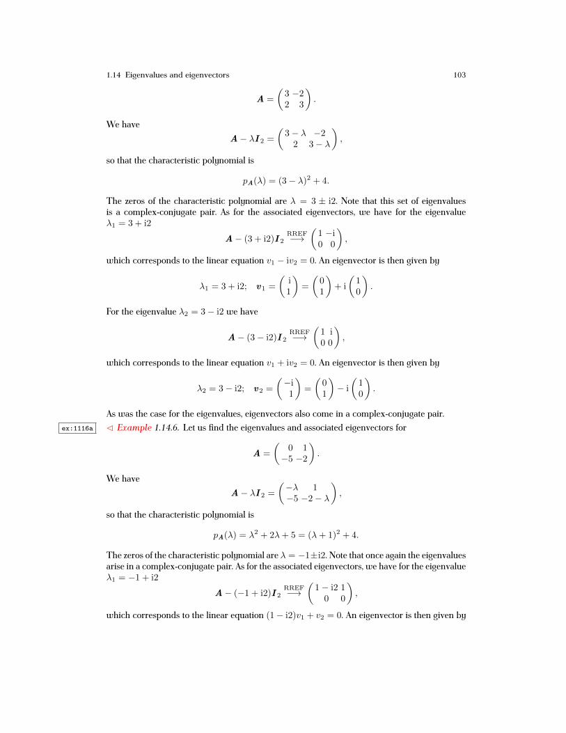
1.14 Eigenvalues and eigenvectors 103
A =
(3 −22 3
).
We haveA− λI 2 =
(3− λ −22 3− λ
),
so that the characteristic polynomial is
pA(λ) = (3− λ)2 + 4.
The zeros of the characteristic polynomial are λ = 3 ± i2. Note that this set of eigenvaluesis a complex-conjugate pair. As for the associated eigenvectors, we have for the eigenvalueλ1 = 3 + i2
A− (3 + i2)I 2RREF−→
(1 −i0 0
),
which corresponds to the linear equation v1 − iv2 = 0. An eigenvector is then given by
λ1 = 3 + i2; v1 =
(i1
)=
(01
)+ i
(10
).
For the eigenvalue λ2 = 3− i2 we have
A− (3− i2)I 2RREF−→
(1 i0 0
),
which corresponds to the linear equation v1 + iv2 = 0. An eigenvector is then given by
λ2 = 3− i2; v2 =
(−i1
)=
(01
)− i
(10
).
As was the case for the eigenvalues, eigenvectors also come in a complex-conjugate pair.ex:1116a C Example 1.14.6. Let us find the eigenvalues and associated eigenvectors for
A =
(0 1−5 −2
).
We haveA− λI 2 =
(−λ 1−5 −2− λ
),
so that the characteristic polynomial is
pA(λ) = λ2 + 2λ+ 5 = (λ+ 1)2 + 4.
The zeros of the characteristic polynomial are λ = −1±i2. Note that once again the eigenvaluesarise in a complex-conjugate pair. As for the associated eigenvectors, we have for the eigenvalueλ1 = −1 + i2
A− (−1 + i2)I 2RREF−→
(1− i2 1
0 0
),
which corresponds to the linear equation (1− i2)v1 + v2 = 0. An eigenvector is then given by

104 1 Essentials of Linear Algebra
λ1 = −1 + i2; v1 =
(−1 + i2
1
)=
(−11
)+ i
(20
).
For the eigenvalue λ2 = −1− i2 we eventually see that an eigenvector is given by
v2 =
(−1− i2
1
)=
(−11
)− i
(20
).
Thus, just as in the previous example the associated eigenvectors also come in a complex-conjugate pair.C Example 1.14.7. We finally consider an example for which the eigenvalues and eigenvectorsmust be computed numerically. Here
A =
1 2 3−1 2 −35 6 7
∈M3(R),
which means that pA(λ) is a third-order polynomial. Unless the problem is very special, it isgenerally the case that it is not possible to (easily) find the three roots. Using WolframAlpha weget
eigenvalues 881,2,3<,8-1,2,-3<,85,6,7<<
Input:
EigenvaluesB1 2 3
-1 2 -3
5 6 7
F
Results: More digits
Λ1 » 5.42882 + 2.79997 ä
Λ2 » 5.42882 - 2.79997 ä
Λ3 » -0.857635
Corresponding eigenvectors: Exact forms More digits
v1 » H0.393543 - 0.0276572 ä, -0.589816 + 0.489709 ä, 1.Lv2 » H0.393543 + 0.0276572 ä, -0.589816 - 0.489709 ä, 1.Lv3 » H-1.99398, 0.352046, 1.L
Generated by Wolfram|Alpha (www.wolframalpha.com) on March 27, 2014 from Champaign, IL.
© Wolfram Alpha LLC— A Wolfram Research Company1
In other words,
λ1 ∼ 5.43 + i2.80, v1 ∼
0.39−0.591.00
+ i
−0.030.490.00
; λ3 ∼ −0.86, v3 ∼
−1.990.351.00
.
1.14 Eigenvalues and eigenvectors 105
The second eigenvalue is the complex-conjugate conjugate of the second, i.e., λ2 = λ1, and theassociated eigenvector is the complex-conjugate of v1, i.e., v2 = v1.
1.14.2 Properties
The last three examples highlight a general phenomena. Suppose that A ∈Mn(R), and furthersuppose that λ = a+ ib is an eigenvalue with associated eigenvector v = p + iq ,
Av = λv A(p + iq) = (a+ ib)(p + iq).
Taking the complex-conjugate of both sides, and using the fact that the conjugate of a productis the product of the conjugates,
Av = Av , λv = λ v ,
givesAv = λ v .
Since A ∈Mn(R), A = A, so we conclude
Av = λv A(p − iq) = (a− ib)(p − iq).
This equation is another eigenvalue/eigenvector equation for the matrix A. The eigenvalue andassociated eigenvector for this equation are related to the original via complex-conjugation. Inconclusion, if A ∈ Mn(R), then the eigenvalues come in the complex-conjugate pairs
{λ, λ
},
i.e., {a± ib}, as do the associated eigenvectors {v , v}, i.e., {p ± iq}.We conclude with some additional facts about eigenvalues and eigenvectors of A ∈Mn(R),
each of which will be useful in applications. First, the eigenvalues tell us something about theinvertibility of the matrix. We first observe that by setting λ = 0,
pA(0) = det(A);
thus, λ = 0 is an eigenvalue if and only if det(A) = 0. Since by Theorem 1.12.9 A is invertibleif and only if det(A) 6= 0, we have that A is invertible if and only if λ = 0 is not an eigenvalue.From Exercise 1.14.4(c) we know that the characteristic polynomial is of degree n; hence, bythe Fundamental Theorem of Algebra there are precisely n eigenvalues. As we have seen in theprevious examples, there may or may not be n linearly independent eigenvectors. However,if the eigenvalues are distinct (each one is algebraically simple), then the n eigenvectors areindeed linearly independent. Since dim[Cn] = n (see Exercise 1.13.7), this means that we canuse the eigenvectors as a basis for Cn.

106 1 Essentials of Linear Algebra
lem:1111 Theorem 1.14.8. Consider the matrix A ∈Mn(R).
(a) If λ = a+ ib is an eigenvalue with associated eigenvector v = p + iq for somevectors p, q ∈ Rn, then the complex-conjugate λ = a− ib is an eigenvalue withassociated complex-conjugated eigenvector v = p − iq .
(b) λ = 0 is an eigenvalue if and only if det(A) = 0.(c) A is invertible if and only if all of the eigenvalues are nonzero.(d) If the eigenvalues λ1, λ2, . . . , λn are distinct, i.e., all of the roots of the char-
acteristic polynomial are simple, then a set of corresponding eigenvectors{v1, v2, . . . , vn} forms a basis for Cn.
Proof. We only need to show that if the eigenvalues are distinct, then the set of correspondingeigenvectors forms a basis. Recall equation (1.14.1),
Av j = λjv j , j = 1, . . . , n.
Set S = Span {v1, . . . , vn}, and suppose dim[S] = r < n. Assume without loss of generalitythat the set {v1, . . . , vr} is linearly independent. This means that the remaining eigenvectorsare each a linear combination; in particular, there exist constants c1, . . . , cr (not all zero) suchthat
vr+1 = c1v1 + c2v2 + · · ·+ crvr. (1.14.2) e:1138aa
Multiplying both sides by A and using the linearity of matrix/vector multiplication gives
Avr+1 = c1Av1 + c2Av2 + · · ·+ crAvr,
which in turn implies
λr+1vr+1 = c1λ1v1 + c2λ2v2 + · · ·+ crλrvr.
Multiplying equation (1.14.2) by λr+1 and subtracting from this the above equation yields
c1(λr+1 − λ1)v1 + c2(λr+1 − λ2)v2 + · · ·+ cr(λr+1 − λr)vr = 0 .
Since the eigenvalues are distinct, i.e., λr+1 − λj 6= 0 for j = 1, . . . , r, and since not all ofthe constants cj are equal to zero, we conclude that the vectors v1, v2, . . . , vr are linearlydependent. This is a contradiction. Hence, we cannot write the eigenvector vr+1 as a linearcombination of the other eigenvectors. The assumption that r < n is false, and consequentlyr = n. ut
1.14.3 Eigenvectors as a basis, and Fourier expansions
The moniker Fourierappeared inChapter 1.9 whenwe discussedorthonormal bases.We use it again herebecause in someinstances - e.g.,A = AT -eigenvectors can bescaled to form anorthonormal basis.
As we will see in the upcoming case studies, as well as our study of linear systems of ODEs,it is extremely beneficial to write a given vector in terms of a linearly independent set of eigen-vectors of a given matrix. For a given matrix A ∈ Mn(R), suppose that a set of eigenvectors,{v1, v2, . . . , vn}, forms a basis. We know from Theorem 1.14.8(d) that this is possible if theeigenvalues are distinct. Going back to our discussion in Chapter 1.8 we then know that anyvector x ∈ Cn can be uniquely written through the expansion

1.14 Eigenvalues and eigenvectors 107
x = c1v1 + c2v2 + · · ·+ cnvn. (1.14.3) e:fourexp
Such an expansion in terms of eigenvectors is sometimes called a Fourier expansion, andthe weights are sometimes called the Fourier coefficients. The Fourier coefficients are foundthrough the solution of the linear system, i.e.,
c1v1 + c2v2 + · · ·+ cnvn = Pc, P = (v1 v2 · · · vn),
meansx = Pc c = P−1x .
The matrix P is invertible because the chosen eigenvectors are assumed to be linearly inde-pendent (otherwise, they would not form a basis), and the result of Theorem 1.12.10 states thatthe inverse exists if and only if the matrix has full rank.
By writing a given vector through a Fourier expansion we develop greater insight into thegeometry associated with matrix/vector multiplication. Multiplying both sides of (1.14.3) by Aand using linearity gives
Ax = c1Av1 + c2Av2 + · · ·+ cnAvn.
Since each vector v j is an eigenvector with associated eigenvalue λj , i.e., Av j = λjv j , we canrewrite the right-hand side of the above as
c1Av1 + c2Av2 + · · ·+ cnAvn = c1λ1v1 + c2λ2v2 + · · ·+ cnλnvn.
Putting the pieces together yields
x = c1v1 + c2v2 + · · ·+ cnvn Ax = c1λ1v1 + c2λ2v2 + · · ·+ cnλnvn.
Thus, the Fourier coefficients associated with the vector Ax are a scaling of those for the vectorx , where the scaling is the eigenvalue associated with the associated eigenvector.
lem:fourexp Lemma 1.14.9. Suppose that for A ∈ Mn(R) there is a set of linearly independenteigenvectors, {v1, v2, . . . , vn} (guaranteed if the eigenvalues are distinct). For anyx ∈ Cn there is the Fourier expansion
x = c1v1 + c2v2 + · · ·+ cnvn,
where the Fourier coefficients c1, c2, . . . , cn are uniquely determined. Moreover, thevector Ax has the Fourier expansion
Ax = c1λ1v1 + c2λ2v2 + · · ·+ cnλnvn,
where each λj is the eigenvalue associated with the eigenvector v j .
The above result is known as the spectral decomposition of the matrix A. While we will notgo into the details here (see [34, Chapter 7.2]), it turns out to be the case that if all the eigenvaluesare real, there exist unique vectors w j such that the Fourier coefficients are given by
cj = wTj x , j = 1, . . . , n.
Consequently, we can write each term in the sum as

108 1 Essentials of Linear Algebra
cjv j =(wTj x)v j = v j
(wTj x)=(v jw
Tj
)x .
The square matrix Pj = v jwTj ∈Mn(R) has rank one (see Exercise 1.14.6). The matrices Pj
are known as spectral projection matrices. We conclude with
Ax = λ1P1x + λ2P2x + · · ·+ λnPnx ,
which means that original matrix can be written as a weighted sum of rank-one matrices,
A = λ1P1 + λ2P2 + · · ·+ λnPn.
C Example 1.14.10. Consider the matrix
A =
(0 1−8 −6
).
It can be checked that the eigenvalues and associated eigenvectors are
λ1 = −2, v1 =
(1−2
); λ2 = −4, v2 =
(1−4
).
The eigenvectors are clearly linearly independent, so they form a basis. For a particular example,let us find the Fourier coefficients for the vector x = (2 − 7)T. Using (1.14.3) we have(
2−7
)= c1
(1−2
)+ c2
(1−4
)=
(1 1−2 −4
)(c1c2
).
The solution to this linear system is(c1c2
)=
(1 1−2 −4
)−1(2−7
)= −1
2
(−4 −12 1
)(2−7
)=
1
2
(13
).
In other words, the Fourier coefficients are
c1 =1
2, c2 =
3
2,
sox =
1
2v1 +
3
2v2.
Using the result of Lemma 1.14.9 we also know that
Ax =1
2(−2)v1 +
3
2(−4)v2 = −v1 − 6v2.
Exercises
hw:1111 Exercise 1.14.1. Suppose that for a given A ∈ Mn(R) there is a set of linearly independenteigenvectors, {v1, v2, . . . , vn}. Suppose that a given x has the Fourier expansion
x = c1v1 + c2v2 + · · ·+ cnvn.
Defining

1.14 Eigenvalues and eigenvectors 109
A` := A ·A · · ·A︸ ︷︷ ︸` times
,
show that:
(a) A2x = c1λ21v1 + c2λ
22v2 + · · ·+ cnλ
2nvn
(b) A3x = c1λ31v1 + c2λ
32v2 + · · ·+ cnλ
3nvn
(c) if ` ≥ 4, A`x = c1λ`1v1 + c2λ
`2v2 + · · ·+ cnλ
`nvn (Hint: use (a), (b), and induction).
Exercise 1.14.2. Compute by hand the eigenvalues and all corresponding eigenvectors for eachmatrix. If the eigenvalue is complex-valued, write the eigenvector in the form v = p + iq .
(a) A =
(1 −2−2 4
)(b) A =
(3 −22 3
)(c) A =
(2 −63 −7
)(d) A =
(1 4−2 −3
)(e) A =
2 5 −25 2 10 0 −3
(f) A =
3 0 01 −1 2−2 −2 −1
Exercise 1.14.3. In each of the following the characteristic polynomial of A ∈Mn(R) is given.Determine n, list each eigenvalue and its algebraic multiplicity, and state whether or not thematrix is invertible.
(a) pA(λ) = (λ− 3)(λ2 + 2λ+ 5)(λ− 4)2
(b) pA(λ) = λ2(λ+ 3)(λ2 − 4λ+ 13)(λ− 1)4
(c) pA(λ) = (λ+ 5)(λ+ 2)3(λ2 + 6λ+ 25)2
(d) pA(λ) = λ(λ2 + 9)(λ2 + 25)(λ− 8)
hw:1112 Exercise 1.14.4. Suppose thatA ∈Mn(C), and let pA(λ) = det(A−λI n) be the characteristicpolynomial.
(a) If n = 2, show that pA(λ) is a polynomial of degree two.(b) If n = 3, show that pA(λ) is a polynomial of degree three.(c) Show that pA(λ) is a polynomial of degree n.
Exercise 1.14.5. Suppose that A ∈Mn(C) is invertible. If for the matrix A, λ is an eigenvaluewith associated eigenvector v , show that for the matrix A−1 there is the eigenvalue 1/λ withassociated eigenvector v .
hw:spectralproj Exercise 1.14.6. Suppose that v ,w ∈ Rn. Show that:
(a) vwT ∈Mn(R)(b) rank(vwT) = 1. (Hint: show that the matrix has only one linearly independent column)
Exercise 1.14.7. For each of the following matrices, write the vector x = (4 − 3)T as a linearcombination of eigenvectors. Explicitly give the weights (Fourier coefficients).
(a) A =
(1 −2−2 4
)
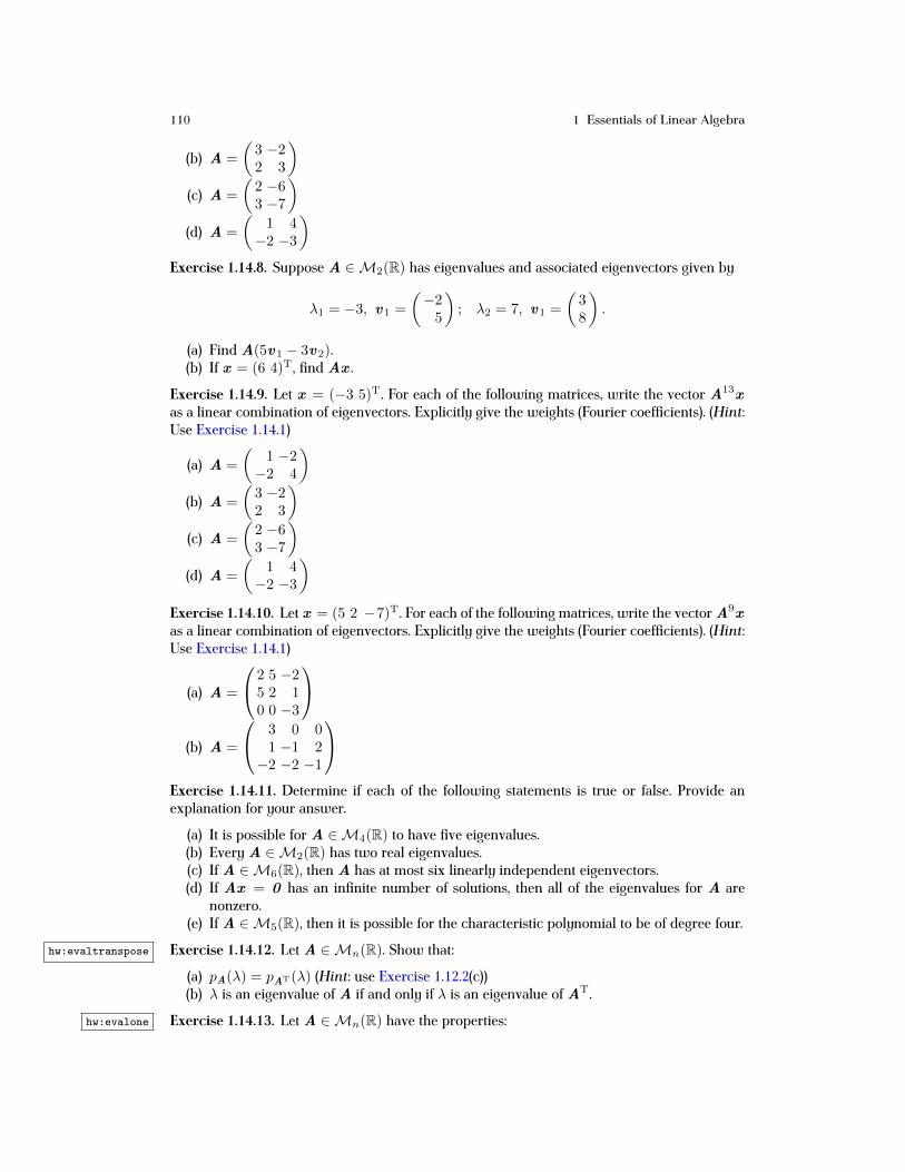
110 1 Essentials of Linear Algebra
(b) A =
(3 −22 3
)(c) A =
(2 −63 −7
)(d) A =
(1 4−2 −3
)Exercise 1.14.8. Suppose A ∈M2(R) has eigenvalues and associated eigenvectors given by
λ1 = −3, v1 =
(−25
); λ2 = 7, v1 =
(38
).
(a) Find A(5v1 − 3v2).(b) If x = (6 4)T, find Ax .
Exercise 1.14.9. Let x = (−3 5)T. For each of the following matrices, write the vector A13xas a linear combination of eigenvectors. Explicitly give the weights (Fourier coefficients). (Hint:Use Exercise 1.14.1)
(a) A =
(1 −2−2 4
)(b) A =
(3 −22 3
)(c) A =
(2 −63 −7
)(d) A =
(1 4−2 −3
)Exercise 1.14.10. Let x = (5 2 −7)T. For each of the following matrices, write the vector A9xas a linear combination of eigenvectors. Explicitly give the weights (Fourier coefficients). (Hint:Use Exercise 1.14.1)
(a) A =
2 5 −25 2 10 0 −3
(b) A =
3 0 01 −1 2−2 −2 −1
Exercise 1.14.11. Determine if each of the following statements is true or false. Provide anexplanation for your answer.
(a) It is possible for A ∈M4(R) to have five eigenvalues.(b) Every A ∈M2(R) has two real eigenvalues.(c) If A ∈M6(R), then A has at most six linearly independent eigenvectors.(d) If Ax = 0 has an infinite number of solutions, then all of the eigenvalues for A are
nonzero.(e) If A ∈M5(R), then it is possible for the characteristic polynomial to be of degree four.
hw:evaltranspose Exercise 1.14.12. Let A ∈Mn(R). Show that:
(a) pA(λ) = pAT(λ) (Hint: use Exercise 1.12.2(c))(b) λ is an eigenvalue of A if and only if λ is an eigenvalue of AT.
hw:evalone Exercise 1.14.13. Let A ∈Mn(R) have the properties:

1.15 Case studies 111
(a) all the entries are nonnegative(b) the sum of the values in each column is one.
Show that:
(a) λ = 1 is an eigenvalue of AT (Hint: consider ATv , where v = (1 1 · · · 1)T)(b) λ = 1 is an eigenvalue of A. (Hint: use the result of Exercise 1.14.12(b))
1.15 Case studiess:212
We now consider three problems in which it soon becomes clear that knowing the eigenvaluesand associated eigenvectors for a given matrix clearly helps in understanding the solution.
1.15.1 Voter registrations:markov
Consider the following table:
D R I
D 0.90 0.03 0.10
R 0.02 0.85 0.20
I 0.08 0.12 0.70
Here R represents Republicans, D Democrats, and I Independents. Let Dj , Rj , Ij representthe number of voters in each group in year j. The table provides information regarding themanner in which voters change their political affiliation from one year to the next. For example,reading down the first column we see that from one year to the next 90% of the Democratsremain Democrats, 2% become Republicans, and 8% become Independents. On the other hand,reading across the first row we see that the number of Democrats in a following year is the sumof 90% of the Democrats, 3% of the Republicans, and 10% of the Independents in the precedingyear.
We wish to know what is the distribution of voters amongst the three groups after manyyears. Using the table we see that the number of voters in each group in year n + 1 given thenumber of voters in each group in year n follows the rule,
Dn+1 = 0.90Dn + 0.03Rn + 0.10In
Rn+1 = 0.02Dn + 0.85Rn + 0.20In
In+1 = 0.08Dn + 0.12Rn + 0.70In.
We implicitly assume here that the total number of voters is constant from one year to the next,so Dn +Rn + In = N for any n, where N is the total number of voters. Upon setting
xn =
Dn
RnIn
, M =
0.90 0.03 0.100.02 0.85 0.200.08 0.12 0.70
,
we can rewrite this as the discrete dynamical system

112 1 Essentials of Linear Algebra
xn+1 = Mxn, x 0 given. (1.15.1) e:1111
The dynamical system (1.15.1) is known as a Markov process, and it is distinguished by the factthat the sum of each column of the transition (stochastic, Markov) matrix M is 1.
For a given initial distribution of voters x 0, we wish to determine the distribution of votersafter many years, i.e., we wish to compute limn→+∞ xn. First, we need to solve for xn. Since
x 1 = Mx 0, x 2 = Mx 1 = M (Mx 0),
by defining M k := MM · · ·M , i.e., M k is the matrix M multiplied by itself k times, we have
x 2 = M 2x 0.
Continuing in this fashion gives
x 3 = Mx 2 = M (M 2x 0) = M 3x 0, x 4 = Mx 3 = M (M 3x 0) = M 4x 0,
so by an induction argument that the solution to the dynamical system is
xn = M nx 0. (1.15.2) e:1111a
Thus, our question is answered by determining limn→+∞M n.We now use the eigenvalues and eigenvectors of M , and the Fourier expansion result of
Lemma 1.14.9, in order to simplify the expression (1.15.2). These quantities are computed usingWolframAlpha using exact arithmetic

1.15 Case studies 113
eigenvalues 889�10,3�100,1�10<,82�100,85�100,2�10<,88�100,12�100,7�10<<
Input:
EigenvaluesB
9
10
3
100
1
10
2
100
85
100
2
10
8
100
12
100
7
10
F
Results: Exact forms
Λ1 � 1
Λ2 » 0.86
Λ3 » 0.59
Corresponding eigenvectors: Approximate forms
v1 �
35
24
,
55
36
, 1
v2 � H-7, 6, 1L
v3 � -1
4
, -3
4
, 1
Generated by Wolfram|Alpha (www.wolframalpha.com) on March 27, 2014 from Champaign, IL.
© Wolfram Alpha LLC— A Wolfram Research Company1
Since the eigenvalues,λ1 = 1, λ2 ∼ 0.86, λ3 ∼ 0.59 (1.15.3) e:cs1eval
are distinct, by Theorem 1.14.8(d) the associated eigenvectors are linearly independent. LettingP = (v1 v2 v3), we know by Lemma 1.14.9 that the initial condition has a Fourier expansionin terms of the eigenvectors,
x 0 = c1v1 + c2v2 + c3v3 = Pc c = P−1x 0. (1.15.4) e:1111b
Now that the initial condition has been written in terms of the eigenvectors we can rewritethe solution in terms of the eigenvalues and eigenvectors. Via the linearity of matrix/vectormultiplication, and using the expansion (1.15.4), we have (1.15.2) can be rewritten as
xn = c1Mnv1 + c2M
nv2 + c3Mnv3. (1.15.5) e:1111aa
Regarding the term M nv `, for each ` = 1, 2, 3
Mv ` = λ`v ` M 2v ` = M (Mv `) = λ`Mv ` = λ2`v `,
which by an induction argument leads to
M nv ` = λn` v `
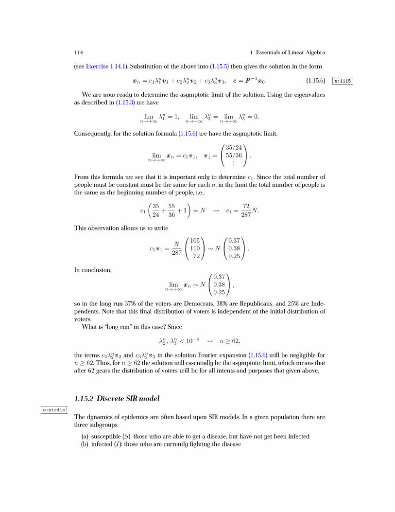
114 1 Essentials of Linear Algebra
(see Exercise 1.14.1). Substitution of the above into (1.15.5) then gives the solution in the form
xn = c1λn1v1 + c2λ
n2v2 + c3λ
n3v3, c = P−1x 0. (1.15.6) e:1115
We are now ready to determine the asymptotic limit of the solution. Using the eigenvaluesas described in (1.15.3) we have
limn→+∞
λn1 = 1, limn→+∞
λn2 = limn→+∞
λn3 = 0.
Consequently, for the solution formula (1.15.6) we have the asymptotic limit,
limn→+∞
xn = c1v1, v1 =
35/2455/36
1
.
From this formula we see that it is important only to determine c1. Since the total number ofpeople must be constant must be the same for each n, in the limit the total number of people isthe same as the beginning number of people, i.e.,
c1
(35
24+
55
36+ 1
)= N c1 =
72
287N.
This observation allows us to write
c1v1 =N
287
10511072
∼ N 0.37
0.380.25
.
In conclusion,
limn→+∞
xn ∼ N
0.370.380.25
,
so in the long run 37% of the voters are Democrats, 38% are Republicans, and 25% are Inde-pendents. Note that this final distribution of voters is independent of the initial distribution ofvoters.
What is “long run” in this case? Since
λn2 , λn3 < 10−4 n ≥ 62,
the terms c2λn2v2 and c3λn3v3 in the solution Fourier expansion (1.15.6) will be negligible forn ≥ 62. Thus, for n ≥ 62 the solution will essentially be the asymptotic limit, which means thatafter 62 years the distribution of voters will be for all intents and purposes that given above.
1.15.2 Discrete SIR models:sirdis
The dynamics of epidemics are often based upon SIR models. In a given population there arethree subgroups:
(a) susceptible (S): those who are able to get a disease, but have not yet been infected(b) infected (I): those who are currently fighting the disease

1.15 Case studies 115
(c) recovered (R): those who have had the disease, or are immune.
Although it is not necessary, it is often assumed that the entire population,
N = S + I +R,
is a constant. Moreover, it is assumed that the number of people in each group does not dependupon location. Consequently, the model to be given is reasonable when looking at epidemics ina school environment, but it not very good when trying to understand nationwide outbreaks ofdisease (which are generally more regional).
Paladini et al. [37] provide a descriptive discrete-time dynamical system of the form
Sn+1 = qSn + cRn
In+1 = (1− q)Sn + bIn
Rn+1 = (1− b)In + (1− c)Rn.(1.15.7) e:sir1
Here Sj is the number of susceptible people in the sampling interval j, Ij is the number ofinfected people in the sampling interval j, and Rj is the number of recovered people in thesampling interval j. Depending upon the disease being studied, the sampling interval may bemonthly, yearly, or even larger. The model assumes that:
(a) susceptible people must become infected before recovering(b) infected people must recover before again becoming susceptible(c) recovered people cannot become infected without first becoming susceptible.
As for the parameters, we have:
(a) 0 ≤ q ≤ 1 is the probability that a susceptible avoids infection(b) 0 ≤ b ≤ 1 is the proportion of individuals which remain infected(c) 0 ≤ c ≤ 1 is the fraction of recovered individuals which lose immunity.
The probability parameter q is generally a function of both S and I , e.g.,
q = 1− p IN,
where p is the probability of the infection being transmitted through a time of contact. We willassume that q is fixed; in particular, we will assume that it does not depend upon the proportionof infected people. It is not difficult to check that
Sn+1 + In+1 +Rn+1 = Sn + In +Rn,
so the total population remains constant for all n (see Exercise 1.15.3). We could use this fact toreduce the number of variables in (1.15.7), but we will not do so in our analysis.
We now proceed to solve (1.15.7). Upon setting
xn =
SnInRn
, A =
q 0 c1− q b 00 1− b 1− c
,
we can rewrite the dynamical system in the form
xn+1 = Axn. (1.15.8) e:sir2

116 1 Essentials of Linear Algebra
Note that this dynamical system shares (at least) one feature with the Markov process associatedwith the voter registration problem: the sum of each column of the matrix A is 1. By followingthe argument leading to (1.15.2) we know the solution is
xn = Anx 0.
Moreover, we know that the eigenvalues and associated eigenvectors of A can be used to sim-plify the form of the solution. Writing Av j = λjv j for j = 1, 2, 3, we know that the solutioncan be written
xn = c1λn1v1 + c2λ
n2v2 + c3λ
n3v3. (1.15.9) e:sir3
The underlying assumption leading to the solution formula in (1.15.9), which will be verifiedfor specific values of b, c, q, is that the eigenvectors are linearly independent. We then know byLemma 1.14.9 that the initial condition x 0 has the Fourier expansion
x 0 = c1v1 + c2v2 + c3v3,
and the Fourier coefficients are found by solving the linear system
Pc = x 0 c = P−1x 0, P = (v1 v2 v3) .
We are now ready to determine the asymptotic limit of the solution. Following [37] we willassume
b = 0.5, c = 0.01.
If we further assume q = 0.2, then the matrix A becomes
A =
0.2 0 0.010.8 0.5 00 0.5 0.99
.
Using WolframAlpha and exact arithmetic we find the eigenvalues and associated eigenvectorsto be:

1.15 Case studies 117
eigenvalues 882�10,0,1�100<,88�10,5�10,0<,80,5�10,99�100<<
Input:
EigenvaluesB
2
100
1
100
8
10
5
100
05
10
99
100
F
Results: Exact forms
Λ1 � 1
Λ2 » 0.47159
Λ3 » 0.21841
Corresponding eigenvectors: Approximate forms
v1 �
1
80
,
1
50
, 1
v2 �
1
100
K29 - 641 O,
1
100
K-129 + 641 O, 1
v3 �
1
100
K29 + 641 O,
1
100
K-129 - 641 O, 1
Alternate form:
:1,
69
200
+641
200
,
69
200
-641
200
>
Generated by Wolfram|Alpha (www.wolframalpha.com) on June 3, 2014 from Champaign, IL.
© Wolfram Alpha LLC— A Wolfram Research Company1
Because the eigenvalues are distinct,
λ1 = 1, λ2 ∼ 0.47, λ3 ∼ 0.22,
we know that the associated eigenvectors are linearly independent.Since
limn→+∞
λn1 = 1, limn→+∞
λn2 = limn→+∞
λn3 = 0,
we have the asymptotic limit
limn→+∞
xn = c1v1, v1 =
1/801/501
.
We see that we now must determine c1. Since the total number of people is constant for all n,in the limit the total number of people is the same as the beginning number of people, whichleads to
c1
(1
80+
1
50+ 1
)= N c1 =
400
413N.
This observation allows us to write

118 1 Essentials of Linear Algebra
c1v1 =N
413
58
400
∼ N0.012
0.0190.969
.
In conclusion,
limn→+∞
xn = N
0.0120.0190.969
,
so in the long run 1.2% of the people are susceptible, 1.9% of the people are infected, and 96.9%of the people are recovered. Note that this final distribution of the population is independent ofthe number of people who were originally infected.
What is “long run” in this case? Since
λn2 , λn3 < 10−4 n ≥ 13,
the terms c2λn2v2 and c3λn3v3 in the solution Fourier expansion (1.15.6) will be negligible forn ≥ 13. Thus, for n ≥ 13 the solution will essentially be the asymptotic limit, which meansthat after 13 sampling intervals the distribution of people will be for all intents and purposesthat given above.
1.15.3 Northern spotted owls:owl
The size of the Northern spotted owl population is closely associated with the health of themature and old-growth coniferous forests in the Pacific Northwest. Over the last few decadesthere has been loss and fragmentation of these forests, which may potentially effect the long-term survival of this species of owl. For spotted owls there are three distinct groupings:
(a) juveniles (j) under one year old(b) subadults (s) between one and two years old(c) adults (a) two years old and older.
The owls mate during the latter two life stages, and begin breeding as adults.In year n let jn be the number of juveniles, sn be the number of subadults, and an be the
number of adults. Mathematical ecologists have modeled a particular spotted owl populationvia the discrete dynamical system
jn+1 = 0.33an
sn+1 = 0.18jn
an+1 = 0.71sn + 0.94an.
The juvenile population in the next year is 33% of the adult population, 18% of the juveniles inone year become subadults in the next year, 71% of the subadults in one year become adultsthe next year, and 94% of the adults survive from one year to the next (see Lamberson et al. [26],Lay [27, Chapter 5], and the references therein). Upon setting
xn =
jnsnan
,
we can rewrite this dynamical system in the form

1.15 Case studies 119
xn+1 = Axn, A =
0 0 0.330.18 0 00 0.71 0.94
. (1.15.10) e:owl1
For a given initial distribution of owls, we wish to see what is the distribution of the owlsafter many years. We first solve for xn in terms of x 0. Following the argument leading to (1.15.2)we know the solution is
xn = Anx 0. (1.15.11) e:owl2
Following our discussion in the previous case study, we know that we next wish to use theeigenvalues and associated eigenvectors for the matrix A. These quantities are computed usingWolframAlpha using exact arithmetic (the exact expressions are not shown)
eigenvalues 880,0,33�100<,818�100,0,0<,80,71�100,94�100<<
Input:
EigenvaluesB
0 033
100
18
1000 0
071
100
94
100
F
Results: More digits
Λ1 » 0.983593
Λ2 » -0.0217964 + 0.205918 ä
Λ3 » -0.0217964 - 0.205918 ä
Corresponding eigenvectors: Exact forms More digits
v1 » H0.335505, 0.0613982, 1.Lv2 » H-0.167752 - 1.58482 ä, -1.35464 + 0.290026 ä, 1.Lv3 » H-0.167752 + 1.58482 ä, -1.35464 - 0.290026 ä, 1.L
Alternate form:
:1
1 500 000
470 000 + 174 991 625 000 000 000 - 3 375 000 000 000 1 742 033 7773
+
5000 1 399 933 + 27 1 742 033 7773
,
root of 500 000 x3
- 470 000 x2
- 21 087 near x � -0.0217964 + 0.205918 ä ,
root of 500 000 x3
- 470 000 x2
- 21 087 near x � -0.0217964 - 0.205918 ä >
Generated by Wolfram|Alpha (www.wolframalpha.com) on March 27, 2014 from Champaign, IL.
© Wolfram Alpha LLC— A Wolfram Research Company1
In particular, the eigenvalues are
λ1 ∼ 0.98, λ2 ∼ −0.02 + i0.21, λ3 ∼ −0.02− i0.21.
By following the logic leading to (1.15.6) we know the solution is
xn = c1λn1v1 + c2λ
n2v2 + c3λ
n3v3, x 0 = c1v1 + c2v2 + c3v3. (1.15.12) e:owl6
Because the eigenvectors are complex-valued, the Fourier coefficients may also be.The asymptotic behavior of the solution depends on the size of the eigenvalues. Looking back
to the solution formula (1.15.12), we need to understand what happens when we take successivepowers of the eigenvalues. While we understand what λn1 means, we do not have an intuitive

120 1 Essentials of Linear Algebra
understanding as to what it means when we write λn2 and λn3 . Recall that we showed in (1.13.1)complex numbers z = a+ ib can be written in the polar form
z = |z|eiθ; eiθ = cos θ + i sin θ, tan θ =b
a.
The polar representation of complex numbers allows us to write
zn = |z|n(eiθ)n
= |z|neinθ.
In particular, we have
λ2 = 0.21ei0.53π λn2 = 0.21nei0.53nπ
λ3 = 0.21e−i0.53π λn3 = 0.21ne−i0.53nπ.
Since|eiθ| = 1 |einθ| = |eiθ|n = 1,
the magnitude of zn is controlled solely by the magnitude of z,
|zn| = |z|n∣∣einθ∣∣ = |z|n.
Thus, in our example it will be the case that |λn2 | = |λn3 | < 10−4 for n ≥ 6. Going back to thesolution formula (1.15.12), we see that for n ≥ 6 we can write it as
xn ∼ 0.98n c1v1.
In order to properly interpret this solution formula, we first want to write the eigenvector v1
so that each entry corresponds to the percentage of the total owl population in each subgroup.This requires that the entries of the eigenvector sum to one. Unfortunately, WolframAlpha doesnot present an eigenvector with that property; instead, we get
v1 ∼
0.33550.06131.0000
.
We know that eigenvectors are not unique, and can be scaled in any desired fashion. We findthe rescaled version of the eigenvector using WolframAlpha
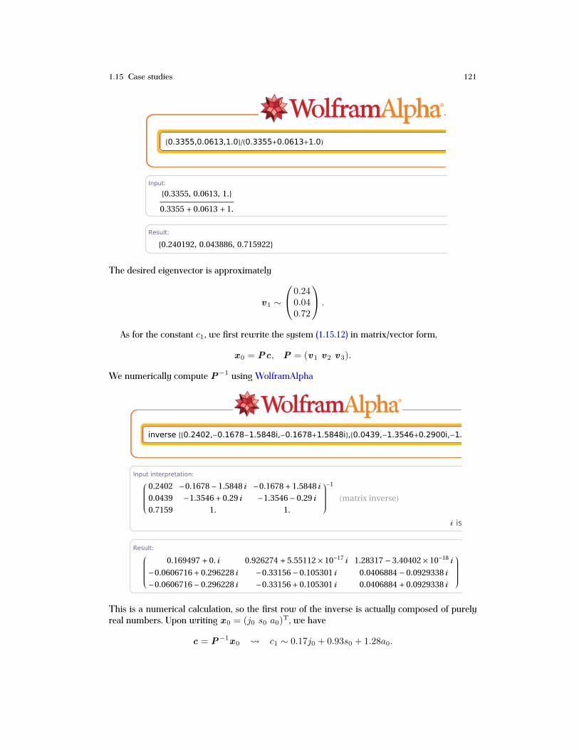
1.15 Case studies 121
80.3355,0.0613,1.0<�H0.3355+0.0613+1.0L
Input:
80.3355, 0.0613, 1.<
0.3355 + 0.0613 + 1.
Result:
80.240192, 0.043886, 0.715922<
Total:
0.240192 + 0.043886 + 0.715922 � 1.
Vector length:
0.756414
Normalized vector:
H0.31754, 0.0580185, 0.946468L
Pie chart:
0.72
0.24
0.044
0.72 H71.6%L
0.24 H24.0%L
0.044 H4.4%L
Spherical coordinates Hradial, polar, azimuthalL:
r » 0.756414 , Θ » 18.8322 ° , Φ » 10.3544 °
Generated by Wolfram|Alpha (www.wolframalpha.com) on March 27, 2014 from Champaign, IL.
© Wolfram Alpha LLC— A Wolfram Research Company1
The desired eigenvector is approximately
v1 ∼
0.240.040.72
.
As for the constant c1, we first rewrite the system (1.15.12) in matrix/vector form,
x 0 = Pc, P = (v1 v2 v3).
We numerically compute P−1 using WolframAlpha
inverse 880.2402,-0.1678-1.5848i,-0.1678+1.5848i<,80.0439,-1.3546+0.2900i,-1.3546-0.2900i<,80.7159,1.,1.<<
Input interpretation:
0.2402 -0.1678 - 1.5848 ä -0.1678 + 1.5848 ä
0.0439 -1.3546 + 0.29 ä -1.3546 - 0.29 ä
0.7159 1. 1.
-1
Hmatrix inverseL
ä is the imaginary unit »
Result:
0.169497 + 0. ä 0.926274 + 5.55112 ´ 10-17
ä 1.28317 - 3.40402 ´ 10-18
ä
-0.0606716 + 0.296228 ä -0.33156 - 0.105301 ä 0.0406884 - 0.0929338 ä
-0.0606716 - 0.296228 ä -0.33156 + 0.105301 ä 0.0406884 + 0.0929338 ä
Dimensions:
3 HrowsL ´ 3 HcolumnsL
Matrix plot:
1 2 3
1
2
3
1 2 3
1
2
3
Determinant: Step-by-step solution
-1.38778 ´ 10-17
- 0.292237 ä
Trace:
-0.121374 - 0.0123673 ä
Characteristic polynomial:
-H0.121374 + 0.0123673 äL x2
- H0.0847487 + 0.0334319 äL x - x3
+ I1.11022 ´ 10-16
- 0.292237 äM
Eigenvalues:
Λ1 » -0.0589837 + 0.698472 ä
Λ2 » -0.569921 - 0.34344 ä
Λ3 » 0.507531 - 0.367399 ä
Generated by Wolfram|Alpha (www.wolframalpha.com) on March 27, 2014 from Champaign, IL.
© Wolfram Alpha LLC— A Wolfram Research Company1
This is a numerical calculation, so the first row of the inverse is actually composed of purelyreal numbers. Upon writing x 0 = (j0 s0 a0)
T, we have
c = P−1x 0 c1 ∼ 0.17j0 + 0.93s0 + 1.28a0.

122 1 Essentials of Linear Algebra
In conclusion, we have
c1v1 ∼ [0.17j0 + 0.93s0 + 1.28a0]
0.240.040.72
.
Thus, for n ≥ 6 we can say
xn ∼ 0.98n[0.17j0 + 0.93s0 + 1.28a0]
0.240.040.72
.
Roughly 24% of the owls will be juveniles, 4% of the owls will be subadults, and 72% of the owlswill be adults. The total number of owls in each group will depend on the initial distribution.The overall population will slowly decrease, and assuming no changes in the conditions leadingto the original model (1.15.10) the owls will eventually become extinct (e.g., 0.98n ≤ 0.1 forn ≥ 114).
Exercises
Exercise 1.15.1. Consider the below table, which represents the fraction of the population ineach group - City (C), and Suburban (S) - which migrates to a different group in a given year.Assume that the total population is constant. Further assume that there are initially 1500 citydwellers, and 1000 suburbanites.
(a) How many people will there be in each group after many years? Assume that the totalnumber of people is constant.
(b) Does your answer in (a) depend on the initial number of people in each group?
C S
C 0.94 0.15
S 0.06 0.85
Exercise 1.15.2. Consider the below table, which represents the fraction of the population ineach group - City (C), Suburban (S), and Rural (R) - which migrates to a different group in agiven year. Assume that the total population is constant. Further assume that there are initially1000 city dwellers, 750 suburbanites, and 250 rural dwellers.
(a) How many people will there be in each group after many years? Assume that the totalnumber of people is constant.
(b) Does your answer in (a) depend on the initial number of people in each group?
C S R
C 0.91 0.09 0.02
S 0.05 0.87 0.08
R 0.04 0.04 0.90
hw:sir1 Exercise 1.15.3. Consider the SIR model given in (1.15.7).
(a) Show that the model supports that the total population is fixed, i.e., show that Sn+ In+Rn = S0 + I0 +R0 for all n ≥ 1.
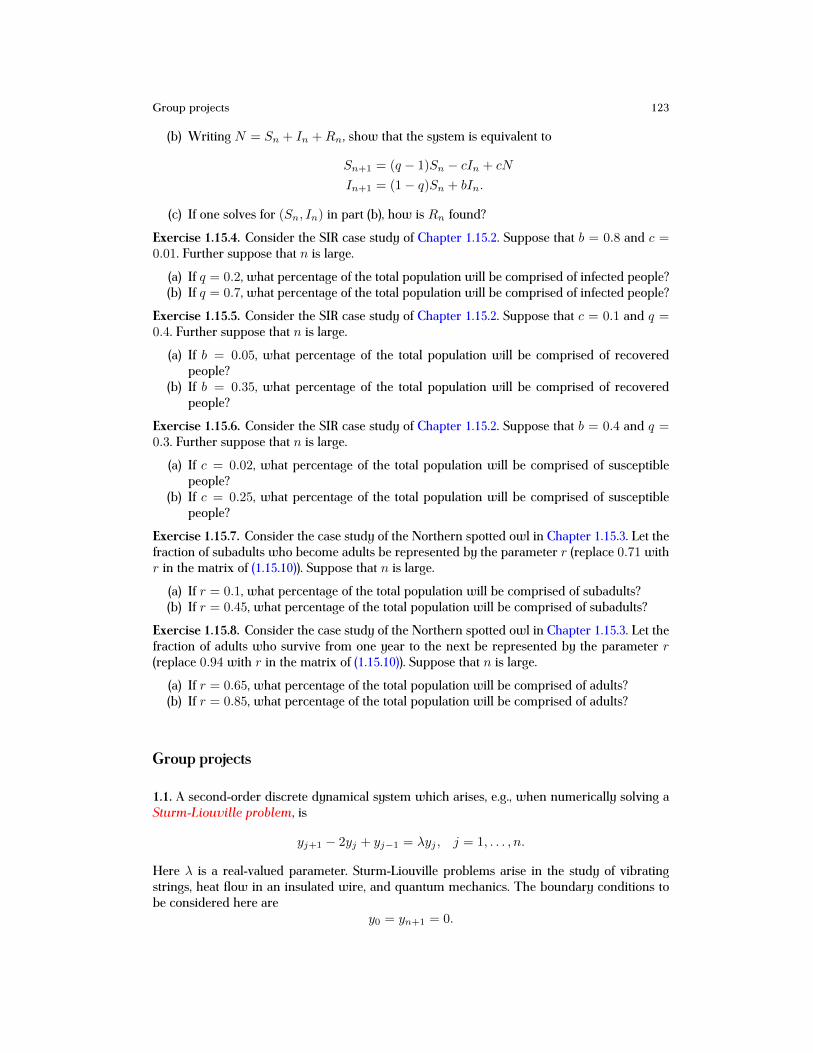
Group projects 123
(b) Writing N = Sn + In +Rn, show that the system is equivalent to
Sn+1 = (q − 1)Sn − cIn + cN
In+1 = (1− q)Sn + bIn.
(c) If one solves for (Sn, In) in part (b), how is Rn found?
Exercise 1.15.4. Consider the SIR case study of Chapter 1.15.2. Suppose that b = 0.8 and c =0.01. Further suppose that n is large.
(a) If q = 0.2, what percentage of the total population will be comprised of infected people?(b) If q = 0.7, what percentage of the total population will be comprised of infected people?
Exercise 1.15.5. Consider the SIR case study of Chapter 1.15.2. Suppose that c = 0.1 and q =0.4. Further suppose that n is large.
(a) If b = 0.05, what percentage of the total population will be comprised of recoveredpeople?
(b) If b = 0.35, what percentage of the total population will be comprised of recoveredpeople?
Exercise 1.15.6. Consider the SIR case study of Chapter 1.15.2. Suppose that b = 0.4 and q =0.3. Further suppose that n is large.
(a) If c = 0.02, what percentage of the total population will be comprised of susceptiblepeople?
(b) If c = 0.25, what percentage of the total population will be comprised of susceptiblepeople?
Exercise 1.15.7. Consider the case study of the Northern spotted owl in Chapter 1.15.3. Let thefraction of subadults who become adults be represented by the parameter r (replace 0.71 withr in the matrix of (1.15.10)). Suppose that n is large.
(a) If r = 0.1, what percentage of the total population will be comprised of subadults?(b) If r = 0.45, what percentage of the total population will be comprised of subadults?
Exercise 1.15.8. Consider the case study of the Northern spotted owl in Chapter 1.15.3. Let thefraction of adults who survive from one year to the next be represented by the parameter r(replace 0.94 with r in the matrix of (1.15.10)). Suppose that n is large.
(a) If r = 0.65, what percentage of the total population will be comprised of adults?(b) If r = 0.85, what percentage of the total population will be comprised of adults?
Group projects
1.1. A second-order discrete dynamical system which arises, e.g., when numerically solving aSturm-Liouville problem, is
yj+1 − 2yj + yj−1 = λyj , j = 1, . . . , n.
Here λ is a real-valued parameter. Sturm-Liouville problems arise in the study of vibratingstrings, heat flow in an insulated wire, and quantum mechanics. The boundary conditions tobe considered here are
y0 = yn+1 = 0.

124 Group projects
One solution to this problem is the trivial solution, yj = 0 for j = 1, . . . , n, and it is valid forany value of λ. The goal is find those values of λ for which there is a nontrivial solution.
(a) Setting
y =
y1y2...yn
∈ Rn,
find the symmetric matrix A so that the problem can be rewritten
Ay = λy .
(b) Suppose that n = 2. Find the eigenvalues and associated eigenvectors.
The remaining questions are devoted to finding an explicit expression for the eigenvalues ifn ≥ 3.
(c) Set h = 1/(n+ 1), and for an as yet unknown α write
yj = eiαjh = cos(αjh) + i sin(αjh).
By using the original system show that
eiα(j+1)h + eiα(j−1)h = (2 + λ)eiαjh.
(d) Solve the equation in part (c) and show that
λ = −2 (1− cos(αh)) .
(e) As written the eigenvector y is complex-valued,
y =
cos(αh)cos(2αh)
...cos(nαh)
+ i
sin(αh)sin(2αh)
...sin(nαh)
= p + iq .
Use linearity to show that the real part, p , and the imaginary part, q , are both real-valuedeigenvectors associated with the real eigenvalue given in part (d).
(f) Use the boundary condition at j = 0, y0 = 0, to conclude the physically relevant eigen-vector is
q =
sin(αh)sin(2αh)
...sin(nαh)
.
(g) Use the boundary condition at j = n+ 1, yn+1 = 0, to determine the values of α whichlead to a nontrivial solution.
(h) What are the eigenvalues λ1, λ2, . . . , λn for the matrix A?
1.2. LetS ∈Mn(R) be a symmetric matrix,ST = S . We will suppose that all of the eigenvaluesare distinct. While we will not prove it, the eigenvalues must be real; hence, we can order them,

Group projects 125
λ1 < λ2 < · · · < λn.
The associated eigenvectors will be denoted v j for j = 1, . . . , n. Recall the definition of aninner-product given in Definition 1.9.1.
(a) Show that 〈Sx ,y〉 = 〈x ,Sy〉. (Hint: consider Exercise 1.10.8 and Exercise 1.10.9)(b) Show that the associated eigenvectors are orthogonal, 〈v i, v j〉 = 0 for i 6= j. (Hint:
consider the quantity 〈Sv i, v j〉, and use part (a))(c) From part (b) we can normalize the eigenvectors to be orthonormal,
〈v i, v j〉 =
{0, i 6= j
1, i = j.
If for a given vector x we write the Fourier expansion,
x = c1v1 + c2v2 + · · ·+ cnvn,
what are the coefficients cj for j = 1, . . . , n?(d) What is the Fourier expansion for Sx ? How do the coefficients for Sx relate to those of
x ?(e) Find an expression for 〈Sx ,x 〉 in terms of the eigenvalues, λ1, . . . , λn, and coefficients,
c1, . . . , cn.(f) If λ1 > 0, i.e., if all of the eigenvalues are positive, show that 〈Sx ,x 〉 > 0 for any vector
x .(g) If λn < 0, i.e., if all of the eigenvalues are negative, show that 〈Sx ,x 〉 < 0 for any vector
x .
1.3. A state-space model of a control system includes a difference equation of the form
xk+1 = Axk + ukb, k = 0, 1, . . . .
Here A ∈Mn(R) and b ∈ Rn. The vector xk is the state vector at “time” k, and the scalar ukis a control or input at time k. The pair (A, b) is said to be controllable if for a given final state,x f , there is a sequence of control scalars {u0, u1, . . . , un−1} such that xn = x f .
(a) For a given initial state x 0, find the state:
• x 1
• x 2
• xn for n ≥ 3.
Write your solution only in terms of the initial state x 0 and the control scalars.(b) Rewrite your solution formula for xn in the form,
xn = C 0x 0 +C 1u ,
for some matrices C 0,C 1 ∈ Mn(R), and some vector u ∈ Rn which depends uponthe input sequence.
(c) Show that the system is controllable if and only if
rank(An−1b An−2b · · · Ab b
)= n.
(d) Set
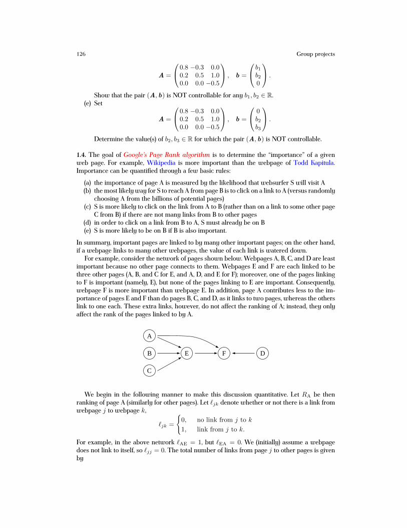
126 Group projects
A =
0.8 −0.3 0.00.2 0.5 1.00.0 0.0 −0.5
, b =
b1b20
.
Show that the pair (A, b) is NOT controllable for any b1, b2 ∈ R.(e) Set
A =
0.8 −0.3 0.00.2 0.5 1.00.0 0.0 −0.5
, b =
0b2b3
.
Determine the value(s) of b2, b3 ∈ R for which the pair (A, b) is NOT controllable.
1.4. The goal of Google’s Page Rank algorithm is to determine the “importance” of a givenweb page. For example, Wikipedia is more important than the webpage of Todd Kapitula.Importance can be quantified through a few basic rules:
(a) the importance of page A is measured by the likelihood that websurfer S will visit A(b) the most likely way for S to reach A from page B is to click on a link to A (versus randomly
choosing A from the billions of potential pages)(c) S is more likely to click on the link from A to B (rather than on a link to some other page
C from B) if there are not many links from B to other pages(d) in order to click on a link from B to A, S must already be on B(e) S is more likely to be on B if B is also important.
In summary, important pages are linked to by many other important pages; on the other hand,if a webpage links to many other webpages, the value of each link is watered down.
For example, consider the network of pages shown below. Webpages A, B, C, and D are leastimportant because no other page connects to them. Webpages E and F are each linked to bethree other pages (A, B, and C for E, and A, D, and E for F); moreover, one of the pages linkingto F is important (namely, E), but none of the pages linking to E are important. Consequently,webpage F is more important than webpage E. In addition, page A contributes less to the im-portance of pages E and F than do pages B, C, and D, as it links to two pages, whereas the otherslink to one each. These extra links, however, do not affect the ranking of A; instead, they onlyaffect the rank of the pages linked to by A.
A
B DFE
C
We begin in the following manner to make this discussion quantitative. Let RA be thenranking of page A (similarly for other pages). Let `jk denote whether or not there is a link fromwebpage j to webpage k,
`jk =
{0, no link from j to k
1, link from j to k.
For example, in the above network `AE = 1, but `EA = 0. We (initially) assume a webpagedoes not link to itself, so `jj = 0. The total number of links from page j to other pages is givenby

Group projects 127
nj =∑k
`jk.
For example, in the above network,
nA = 2, nE = 1, nF = 0.
The ranking of a webpage will be defined to be the weighted sum of the number of numberof links from other pages, with the weight being the ratio of the page rank and total number oflinks,
Rj =∑k
`kjnk
Rk.
For example, in the sample network,
RA = 0, RE =1
2RA +RB +RC, RF =
1
2RA +RD +RE.
Finally, we assume for the network that the total rank (the sum of all the ranks) is one, so forthe sample system,
RA +RB +RC +RD +RE +RF = 1.
The current model has the problem that a surfer who ends up on a page with no externallinks cannot go to a new page (e.g., page F). For those webpages we will assume that the surferwill choose randomly from any page in the entire network. In other words, if the networkhas N webpages, and webpage j has no links to any other webpages (so initially `jk = 0 fork = 1, . . . , N ), then we will set `jk = 1 for each k. The total number of links then changes from0 to N . For example, in the network shown above we reset `Fk = 1 for k ∈ {A,B,C,D,E,F},so that nF = 6. The modified ranking formula for pages E and F are
RE =1
2RA +RB +RC +
1
6RF, RF =
1
2RA +RD +RE +
1
6RF.
Note well that this modification does not change the requirement that the total rank is one.The revised model still does not take into account that a websurfer might randomly select
a new webpage from the network instead of clicking on a link from the current page. We willlet 0 < d ≤ 1 (the damping factor) denote the probability that a websurfer uses a link onthe current page to get to the next page (1 − d is then the probability that a new page will berandomly selected). If d = 1 the surfer uses only the links to go to the next webpage, and if d = 0the links are never used to go to the next webpage. We will assume that the damping factoris fixed and constant for all webpages. The possibility of randomly selecting a new webpageeffects the general ranking formula via
Rj 7→ dRj +1− dN
= dRj +1− dN
∑k
Rk.
The latter equality follows from the total rank being one. Going back to the specific example,the ranking formula for pages E and F are
RE = d
(1
2RA +RB +RC +
1
6RF
)+
1− d6
(RA +RB +RC +RD +RE +RF)
RF = d
(1
2RA +RD +RE +
1
6RF
)+
1− d6
(RA +RB +RC +RD +RE +RF) .

128 Group projects
For the project, consider the network of eight webpages given below:
1 432
5 876
Set r = (R1 R2 · · · R8)T, where Rj is the rank of page j. Suppose that the damping factor is
d = 0.9.
(a) Find the matrix A ∈M8(R) such that Ar = r .(b) Verify that the matrix has the properties that:
• all the entries are nonnegative• the sum of the values in each column is one.
(c) Show (without using WolframAlpha or some other CAS) that λ = 1 is an eigenvalue ofA. (Hint: Exercise 1.14.12 and Exercise 1.14.13 may be helpful)
(d) Show that the system in (a) has a nonzero solution.(e) The system can be numerically solved using an iterative method (this is preferred for
large networks). Set r0 = (1 0 · · · 0)T, and define the vectors r1, r2, . . . via
rn+1 = Arn.
Give an expression for rn in terms of the initial vector r0. Explain.(f) Determine lim
n→+∞rn. (Hint: it may be helpful to use some of the MATLAB commands
provided for in Chapter 1.15.3 to do the numerical calculations)(g) Is the answer in part (e) a solution to the linear system of part (a)? Why, or why not?(h) What is a value N such that if n ≥ N , then we can expect the difference between rn
and the solution to the linear system of part (a) to be O(10−4)? Describe how you chosethis value of N .
(i) Which webpage is most important, and what is its page rank?(j) Which webpage is least important, and what is its page rank?
Author’s note: the preceding discussion, and facets of this project, were provided to me by Prof.Kelly Mcquighan.
MATLAB support
ch:matlabHere we briefly describe how to use each of the provided MATLAB functions, which are cur-rently available at http://www.calvin.edu/∼tmk5/courses/m231/S14/. Moreover, the in-terested reader can also find there a short MATLAB tutorial developed by Toby Driscoll. Theyare easy to use; indeed, all that is required of the user is an understanding of how to inputmatrices and vectors into MATLAB. Examples are included after each of the programs is brieflydescribed.
In order to use the below linear algebra programs it is only necessary that that the userknow how to enter a matrix and vector in MATLAB. The entries in each row are separated bya comma, and each row is separated by a semi-colon. For example, if we have
A =
(1 2 −3−3 −6 7
), b =
324
then they are entered in MATLAB via the command
>> A=[1,2,-3;-3,-6,7];
>> b=[3;2;4];
The semi-colon at the end of the line suppresses the output. If it is not present, then the enteredmatrix is mirrored. The supplied individual functions are:
• cola: find a basis for the column space of a matrix A by using the command cola(A)
• deta: find the determinant of a matrix A by using the command deta(A)
• evalsa: find the eigenvalues and associated eigenvectors of a matrix A by using thecommand evalsa(A)
• gaussa: find the row reduced echelon form (RREF) of a matrix A by using the commandgaussa(A)
• gaussab: find the RREF of the augmented matrix (A|b) by using the command gaussab(A,b)• inva: find the inverse of a matrix A by using the command inva(A)
• nulla: find a basis for the null space of a matrix A by using the command nulla(A)
• zerop: find the zeros of a polynomial. The input is a row vector which contains thecoefficients of the given polynomial. For example, if the polynomial is
p(x) = 5x4 − 3x2 + 6x+ 8,
then the associated MATLAB commands are
129

130 MATLAB support
>> coef=[5,0,-3,6,8];
>> zerop(coef)
The MATLAB code for dfield8 and pplane8 was developed by John Polking of Rice Uni-versity. This code is also available off Polking’s web site, and is provided here solely for thesake of convenience.
• dfield8: numerically solves scalar ODEs x′ = f(t, x) for initial conditions which canbe either inputted via a keyboard, or via the click of a mouse
• pplane8: numerically solves autonomous planar ODEs x′ = f(x, y), y′ = g(x, y) forinitial conditions which can be either inputted via a keyboard, or via the click of a mouse.
C Example 1.15.1. Consider a linear system for which the coefficient matrix and nonhomoge-neous term are
A =
1 2 34 5 67 8 2
, b =
−14−7
.
We will use the provided MATLAB function gaussab to put the augmented matrix into RREF. Itis straightforward to enter a matrix in MATLAB. The matrix entries are surrounded by squarebrackets. The entries in each row are separated by a comma, and each row is separated by asemi-colon. For this particular example we have the sequence of commands:
>> A=[1,2,3;4,5,6;7,8,2];
>> b=[-1;4;-7];
>> gaussab(A,b)
RREF of (A|b):
1.0000 0 0 6.6190
0 1.0000 0 -7.2381
0 0 1.0000 2.2857
In the first command line we entered the coefficient matrix A, and in the second commandline we enter the vector b . Ending each of these lines with a semi-colon suppresses the output;otherwise, the matrix will be mirrored. Note that in the last command line there is no semi-colon at the end. We interpret the output to say that the linear system is consistent, and theunique solution is approximately
x ∼
6.62−7.242.29
.
C Example 1.15.2. Consider the homogeneous linear system Ax = 0 , where
A =
3 4 7 −12 6 8 −4−5 3 −2 −87 −2 5 9
.
We will use the provided MATLAB command nulla to find a spanning set for Null(A). Inparticular,

MATLAB support 131
>> A=[3,4,7,-1;2,6,8,-4;-5,3,-2,-8;7,-2,5,9];
>> nulla(A)
Basis for Null(A):
-1 -1
-1 1
1 0
0 1
so that
Null(A) = Span{
−1−110
,
−1101
}.C Example 1.15.3. Consider the linear system Ax = b , where
A =
3 4 −7 22 6 9 −2−5 3 2 −137 −2 5 16
, b =
52711−1
.
We will use the provided MATLAB command nulla to find the homogeneous solution, and theprovided MATLAB command gaussab to find a particular solution. Regarding the null spacewe have
>> A=[3,4,-7,2;2,6,9,-2;-5,3,2,-13;7,-2,5,16];
>> b=[5;27;11;-1];
>> nulla(A)
Basis for Null(A):
-2
1
0
1
so
Null(A) = Span{
−2101
}.The homogeneous solution is then
xh = t
−2101
, t ∈ R.
In order to find the particular solution we do not need to reenter the MATLAB expressions forA and b , so we simply type

132 MATLAB support
>> gaussab(A,b)
RREF of (A|b):
1 0 0 2 0
0 1 0 -1 3
0 0 1 0 1
0 0 0 0 0
The particular solution is the last column of the RREF of (A|b), i.e.,
xp =
0310
.
C Example 1.15.4. We now consider an example for which a basis for Col(A) and Null(A)are computed numerically. Here A ∈ R4×4 is given by
A =
1 2 3 4−1 2 1 05 6 11 162 4 6 8
⇒ A = [1, 2, 3, 4;−1, 2, 1, 0; 5, 6, 11, 16; 2, 4, 6, 8];
Using the provided MATLAB function gaussa generates the output:>> gaussa(A)
RREF of A:
1 0 1 2
0 1 1 1
0 0 0 0
0 0 0 0
From this RREF we see that rank(A) = 2, and dim[Null(A)] = 2. In order to numericallygenerate a basis for the column space and null space we use the provided MATLAB functionscola and nulla, respectively, to get:
>> cola(A)
Basis for Col(A):
1 2
-1 2
5 6
2 4
>> nulla(A)
Basis for Null(A):
-1 -2
-1 -1
1 0
0 1
As expected, we get as a basis for Col(A) the first two columns of A. As for the null space wesee that
Null(A) = Span{
−1−110
,
−2−101
}.
MATLAB support 133
C Example 1.15.5. We finally consider an example for which the inverse must be computednumerically. Here A ∈ R3×3, and the calculation will be done using the provided MATLABfunction inva. Using this function for the matrix
A =
1 2 3−1 2 −35 6 7
⇒ A = [1, 2, 3;−1, 2,−3; 5, 6, 7];
generates the following output:
>> inva(A)
Inverse of A:
-1.0000 -0.1250 0.3750
0.2500 0.2500 0
0.5000 -0.1250 -0.1250
In other words, upon using the exact expressions for the numerical approximations we have
A−1 =1
8
−8 −1 32 2 04 −1 −1
.
It is straightforward to check that AA−1 = I 3.C Example 1.15.6. We now calculate the determinant of a matrix using the provided MATLABfunction deta. Using this function for the matrix
A =
1 2 3−1 2 −35 6 7
⇒ A = [1, 2, 3;−1, 2,−3; 5, 6, 7];
we have the following output:
>> deta(A)
det(A): -32
In other words, det(A) = −32.C Example 1.15.7. We finally consider an example for which the eigenvalues and eigenvectorsmust be computed numerically. Here A ∈ R3×3, which means that pA(λ) is a third-orderpolynomial. Unless the problem is very special, it is generally the case that it is not possible to(easily) find the three roots. This calculation will be done using the provided MATLAB functionevalsa. Using this function for the matrix
A =
1 2 3−1 2 −35 6 7
⇒ A = [1, 2, 3;−1, 2,−3; 5, 6, 7];
we have the following output:

134 MATLAB support
>> evalsa(A)
Eigenvalues:
-0.8576 + 0.0000i 5.4288 + 2.8000i 5.4288 - 2.8000i
Eigenvectors:
-0.8830 + 0.0000i -0.2981 + 0.0209i -0.2981 - 0.0209i
0.1559 + 0.0000i 0.4467 - 0.3709i 0.4467 + 0.3709i
0.4428 + 0.0000i -0.7574 + 0.0000i -0.7574 + 0.0000i
In other words,
λ1 ∼ −0.86, v1 ∼
−0.880.160.44
; λ2 ∼ 5.43 + i2.80, v2 ∼
−0.300.45−0.76
+ i
0.02−0.370.00
.
The third eigenvalue is the complex-conjugate conjugate of the second, i.e., λ3 = λ2, and theassociated eigenvector is the complex-conjugate of v2, i.e., v3 = v2.C Example 1.15.8. Let us find the general solution to the scalar ODE,
x′ = −x+ t− 4t3,
using the method of undetermined coefficients. Since f(t) = t − 4t3, which is a third-orderpolynomial, we will guess the particular solution to be
xp(t) = a0 + a1t+ a2t2 + a3t
3.
Plugging this guess into the ODE yields
a1 + 2a2t+ 3a3t2︸ ︷︷ ︸
x′p
= −(a0 + a1t+ a2t2 + a3t
3)︸ ︷︷ ︸−xp
+t− 4t3,
which can be rewritten as
a0 + a1 + (a1 + 2a2 − 1)t+ (a2 + 3a3)t2 + (a3 + 4)t3 = 0.
Since a polynomial can be identically zero if and only all of its coefficients are zero, we then getthe linear system of equations
a0 + a1 = 0, a1 + 2a2 − 1 = 0, a2 + 3a3 = 0, a3 + 4 = 0,
which can be rewritten in matrix form as1 1 0 00 1 2 00 0 1 30 0 0 1
a =
010−4
, a =
a0a1a2a3
.
We use the provided MATLAB function gaussab to solve the linear system via the sequence ofcommands

MATLAB support 135
>> A=[1,1,0,0;0,1,2,0;0,0,1,3;0,0,0,1];
>> b=[0,1,0,-4];
>> gaussab(A,b)
RREF of (A|b):
1 0 0 0 23
0 1 0 0 -23
0 0 1 0 12
0 0 0 1 -4
We conclude
a =
23−2312−4
,
so the particular solution isxp(t) = 23− 23t+ 12t2 − 4t3.
The general solution isx(t) = ce−t + 23− 23t+ 12t2 − 4t3.
C Example 1.15.9. Consider the third-order ODE
y′′′ − 3y′′ + 6y′ + 9y = 0.
The associated characteristic polynomial is
p(λ) = λ3 − 3λ2 + 6λ+ 9.
The roots cannot easily be found analytically. However, they can be found numerically usingthe provided MATLAB function zerop. In general, if the characteristic polynomial is
p(λ) = λn + an−1λn−1 + · · ·+ a1λ+ a0,
the roots of the polynomial are found by first putting the coefficients into a row vector, and thencalling the command. For our particular example, the sequence of commands
>> coef=[1,-3,6,9];
>> zerop(coef)
Roots:
-4.6890 + 0.0000i 0.8445 + 1.0983i 0.8445 - 1.0983i
reveals the three roots to be
λ1 ∼ −4.69, λ2 ∼ 0.84 + i1.10, λ3 ∼ 0.84− i1.10.
Since the roots must come in complex-conjugate pairs, we know the first root is purely real.The general solution is
y(t) = c1e−4.69t + c2e
0.84t cos(1.10t) + c3e0.84t sin(1.10t).


Answers to selected exercises
Chapter 11.1.3 (b) r = 8.
1.1.7 No. There are at least two free variables, so there will always be an infinite number ofsolutions.
1.2.1 (c) The product is not well-defined.
1.2.5 b = t
(1−3
)for any t ∈ R.
1.3.2 5x1 + 2x2 = 0.
1.3.6 (e) NO. The weights are x1 = 3, x2 = −2, x3 = −1.
1.4.1 (d) Span{(−21
)}.
1.4.5 (b) xh = t
−241
for any t ∈ R, and xp =
−320
.
1.5.1 (a) NO. The presence of a zero row in the RREF of A means the linear system will notalways be consistent (see Theorem 1.6.3).
1.5.5 (b) r = −19.
1.5.9 (c) FALSE. Since the null space is nontrivial, there is a nonzero solution to Ax = 0 ,which means that some linear combination of the columns leads to the zero vector.
1.6.2 NO. The zero vector is not contained in the set.
1.7.1 (c) rank(A) = 3 and dim[Null(A)] = 1.
1.7.5 NO. Since dim[R6] = 6, a basis for R6 requires six vectors.
1.7.7 (b) FALSE. The seven vectors must be in R7.
1.8.6 (b) cos θ = 15/√17 · 66.
1.8.15 (b) 12cos(x)− 1
2cos(3x).
137

138 Answers to selected exercises
1.9.1 (e)(
1 −31−17 −26
).
1.9.2 (b) k = m, and BA ∈ Rn×n.
1.9.14 (b) FALSE. While the size of AB and BA are the same, the equality will not alwayshold since matrix multiplication generally does not commute.
1.10.1 (b) The inverse does not exist.
1.10.3 The solution to Ax = b1 is x =1
23
(−1237
).
1.10.6 (e) FALSE. Since the matrix is invertible, the RREF is the identity matrix, which meansthat all of the columns are pivot columns, and hence are linearly independent.
1.11.1 (c) det(A) = −4, and det(A−1) = −1/4.
1.11.10 (b) FALSE. Since there is a unique solution for any b , the matrix is invertible, whichmeans det(A) 6= 0.
1.12.2 (d) z =√37 eiθ , where tan θ = 1/6.
1.12.5 (a) Null(A) = Span{(−4 + i6
1
)}, and dim[Null(A)] = 1.
1.13.2 (c) λ1 = −1 with v1 =
(21
), and λ2 = −4 with v2 =
(11
).
1.13.5 (c) Using the eigenvectors given in Problem 1.13.2(c), x = 7v1 − 10v2.
1.13.8 (b) FALSE. The eigenvalues can be complex-valued with nonzero imaginary part.
1.14.1 (a) limn→+∞
Cn =5
7(2500) ∼ 1786, and lim
n→+∞Sn =
2
7(2500) ∼ 714.
1.14.4 (b) Approximately 4.6%.
1.14.7 (a) Approximately 4.7%.
Chapter 22.1.2 (a) x′ = −ax, where a = − ln(2)/5370.
2.3.1 (a) x(t) = ce3t + cos2(7t) + t2 − 6e5t.
2.4.1 (a) x(t) = cet−t2/2.
2.5.2 (c) x(t) = (t2 − 2t+ 2)et − e + 4
t2.
2.5.4 (c) xp(t) = t(a0 + a1t+ a2t2 + a3t
3)e−t.
2.6.4 t ∼ 643.78 days.
2.6.10 r ∼ 0.012.
Chapter 3

Answers to selected exercises 139
3.1.2 x ′ =
(−6/200 1/2502/200 −9/250
)x +
(25 + 5 cos(2t)63 + 14e−2t
), x (0) =
(1400225
).
3.2.1 (d) x ′ =
0 1)00 0 1−2 −5 8
x +
007t
.
3.3.1 (a) Φ(t) =
(et e−3t
et −3e−3t).
3.5.3 (a) The origin is a stable node.
3.5.6 (c) The origin is an unstable saddle point.
3.5.10 (a) x (t) = c1e−2t(15
)+ c2e
2t
(11
).
3.5.16 (a) The origin is an unstable node.
3.6.3 x (t) = c1et
(21
)+ c2e
3t
(01
)+ e2t
(12
).
3.6.11 xp(t) = 23te2t(13
)+
19
2e2t(14
).
3.7.2 (a) x ′ =(−15/100 10/100
5/100 −15/100
)x +
(5c110c2
); x (0) =
(4050
).
3.7.5 (a) Approximately 15.79% are susceptible, 0.02% are infected, and 84.18% are recoveredor immune.
Chapter 44.1.3 (d) y(t) = c1e
3t + c2e6t.
4.1.5 (a) The ODE is fourth-order, and y(t) = c1et + c2e
−3t + c3te−3t + c4e
5t.
4.2.1 (c) y = c1e−2t + c2e
−5t + 2te−2t.
4.2.3 (a) yp(t) = t2(a0 + a1t)e−t + a2 cos(2t) + a3 sin(2t).
4.2.5 (a) yp(t) = t2(a0 + a1t+ a2t2)et.
4.2.6 (c) y(t) = c1t+ c2t2 + t2 tan−1(t)− 1
2t ln(1 + t2).
4.2.8 (e) y(t) = c1 cos(3 ln(t)) + c2 sin(3 ln(t)).
4.2.9 (c) y(t) = c1t+c2t2− 9
4+
3
2ln(t).
4.4.2 (a) y1(t) =1
2A (cos(ωnt) + cos(ωct)) +
1
2B
(sin(ωnt)
ωn+
sin(ωct)
ωc
)and
y2(t) =1
2A (cos(ωnt)− cos(ωct)) +
1
2B
(sin(ωnt)
ωn− sin(ωct)
ωc
).
Chapter 55.1.1 (b) f(t) = t2 +
(4et − t2
)H(t− 2) + (6− 4et)H(t− 5).

140 Answers to selected exercises
5.3.2 (d) L[f ](s) = − 4
(s+ 3)2+ 6
e−s
s+
4
s− 8
s2.
5.3.3 (f) f(t) =(2e−2(t−3) cos(3(t− 3))− 7
3e−2(t−3) sin(3(t− 3))
)H(t− 3).
5.4.1 (e) yp(t) =3
29
(1− e2(t−2) cos(5(t− 2)) +
2
5e2(t−2) sin(5(t− 2))
)H(t− 2).
5.4.2 (b) yp(t) = −5
3e−4t cos(2t)− 1
3e−4t sin(2t) + 2e−4(t−3) sin(2(t− 3))H(t− 3)
−6e−4(t−5) sin(2(t− 5))H(t− 5).
5.5.3 a = 1 + kπ for k = 1, 2, 3, . . . .
5.6.1 (c) H(s) =[s2 + 8s+ 12
]−1.
5.6.2 (d) yp(t) =∫ t0
(e3(t−u) − e2(t−u)
)f(u) du.
5.6.4 (b) y′′ + 2y′ + 5y = f(t).
Chapter 66.1.1 (c) x(t) = ln (C + et).
6.2.1 (d) x = 0 is stable, x = ±1 are unstable, and x = 3 is semi-stable.
6.4.1 (b) The recursion relationship is aj+1 = aj + 8. The solution is a0∞∑j=0
1
j!tj + 8
∞∑j=1
bjtj ,
where b1 = 1, b2 = 1, b3 = 2/3, b4 = 5/12, . . . .

References 141
References
ablowitz:cvi03 [1] M. Ablowitz and A. Fokas. Complex Variables: Introduction and Applications. Cambridge Textsin Applied Mathematics. Cambridge University Press, 2nd edition, 2003.
ackerman:amm64 [2] E. Ackerman, J. Rosevear, and W. McGuckin. A mathematical model of the glucose tolerance test.Phys. Med. Biol., 9:202–213, 1964.
ackerman:bgr69 [3] E. Ackerman, L. Gatewood, J. Rosevear, and G. Molnar. Blood glucose regulation and diabetes. InF. Heinmets, editor, Concepts and Models of Biomathematics, chapter 4, pages 131–156. MarcelDekker, 1969.
asmar:aca02 [4] N. Asmar. Applied Complex Analysis with Partial Differential Equations. Prentice Hall, 2002.billah:rtn91 [5] K. Billah and R. Scanlan. Resonance, Tacoma Narrows bridge failure, and undergraduate physics
textbooks. Amer. J. Phys., 59:118–124, 1991.blanchard:de12 [6] P. Blanchard, R. Devaney, and G. Hall. Differential Equations. Brooks/Cole, Fourth edition, 2012.boelkins:dew09 [7] M. Boelkins, M. Potter, and J. Goldberg. Differential Equations with Linear Algebra. Oxford
University Press, 2009.bolie:con61 [8] V. Bolie. Coefficients of normal blood glucose regulation. J. Appl. Physiol., 16(5):783–788, 1961.
borrelli:de87 [9] R. Borelli and C. Coleman. Differential Equations: A Modeling Approach. Prentice-Hall, Inc.,1987.
boyce:ede05 [10] W. Boyce and R. DiPrima. Elementary Differential Equations. John Wiley & Sons, Inc., Eighthedition, 2005.
bronson:soo09 [11] R. Bronson and G. Costa. Schaum’s Outline of Differential Equations. Schaum’s Outlines.McGraw-Hill, Third edition, 2009.
brown:cva04 [12] J. Brown and R. Churchill. Complex Variables and Applications. McGraw-Hill, 7th edition, 2004.conrad:dea03 [13] B. Conrad. Differential Equations: A Systems Approach. Pearson Education, Inc., 2003.
courant:mom53 [14] R. Courant and D. Hilbert. Methods of Mathematical Physics, volume 1. Interscience Publishers,Inc., 1953.
drazin:sol89 [15] P. Drazin and R. Johnson. Solitons: an introduction. Cambridge University Press, Cambridge,1989.
edwards:dea08 [16] C. Edwards and D. Penney. Differential Equations and Linear Algebra. Pearson, 3rd edition,2008.
evans:pde98 [17] L. Evans. Partial Differential Equations, volume 19 of Graduate Studies in Mathematics. Amer-ican Mathematical Society, 1998.
eves:emt80 [18] H. Eves. Elementary Matrix Theory. Dover Publications, Inc., 1980.fay:cse03 [19] T. Fay and S. Graham. Coupled spring equations. Int. J. Math. Educ. Sci. Technol., 34(1):65–79,
2003.goode:dea07 [20] S. Goode and S. Annin. Differential Equations and Linear Algebra. Prentice Hall, 2007.
griffiths:nmf10 [21] D. Griffiths and D. Higham. Numerical Methods for Ordinary Differential Equations: InitialValue Problems. Undergraduate Mathematics Series. Springer, 2010.
haberman:apd12 [22] R. Haberman. Applied Partial Differential Equations with Fourier Series and Bounday ValueProblems. Pearson Education, Inc., 5th edition, 2012.
hefferon:la09 [23] J. Hefferon. Linear Algebra. Virginia Commonwealth University Mathematics, 2009.http://joshua.smcvt.edu/linalg.html/.
holmes:itp13 [24] M. Holmes. Introduction to Perturbation Methods, volume 20 of Texts in Applied Mathematics.Springer-Verlag, 2nd edition, 2013.
kaper:mac14 [25] H. Kaper and H. Engler. Mathematics and Climate. SIAM, 2014.lamberson:ada92 [26] R. Lamberson, R. McKelvey, R. Noon, and C. Voss. A dynamic analysis of the viability of the
Northern Spotted Owl in a fragmented forest environment. Conservation Biology, 6:505–512,1992.
lay:laa12 [27] D. Lay. Linear Algebra and its Applications. Pearson, 4th edition, 2012.lebedev:sfa72 [28] N. Lebedev. Special Functions and Their Applications. Dover Publications, Inc., New York,
1972.lipschutz:soo12 [29] S. Lipschutz and M. Lipson. Schaum’s Outline of Linear Algebra. Schaum’s Outlines. McGraw-
Hill, Fifth edition, 2012.logan:apd04 [30] J. D. Logan. Applied Partial Differential Equations. Springer, 2nd edition, 2004.
markushevich:tof85 [31] A. Markushevich. Theory of Functions. Chelsea Publishing Co., New York, 1985.mcbride:anl06 [32] G. McBride and N. French. A new linear analytical SIR model for age-dependent susceptibility and
occupation-dependent immune status. In SMO’06 Proceedings of the 6th WSEAS InternationalConference on Simulation, Modelling and Optimization, pages 222–226. WSEAS, 2006.

142 Answers to selected exercises
meirovitch:ami67 [33] L. Meirovitch. Analytical Methods in Vibrations. MacMillan Series in Applied Mechanics. TheMacMillan Company, New York, 1967.
meyer:maa00 [34] C. Meyer. Matrix Analysis and Applied Linear Algebra. SIAM, 2000.nagle:fod00a [35] R. Nagle, E. Saff, and A. Snider. Fundamentals of Differential Equations. Addison-Wesley, Fifth
edition, 2000.oppenheim:sas96 [36] A. Oppenheim, A. Willsky, and S. Hamid. Signals and Systems. Prentice Hall, 2nd edition, 1996.paladini:ads11 [37] F. Paladini, I. Renna, and L. Renna. A discrete SIRS model with kicked loss of immunity and
infection probability. J. Phys.: Conf. Ser., 285:012018, 2011.perko:dea96 [38] L. Perko. Differential Equations and Dynamical Systems. Springer-Verlag, 2nd edition, 1996.
polking:ode03 [39] J. Polking. Ordinary Differential Equations Using MATLAB. Pearson, 3rd edition, 2003.strogatz:nda94 [40] S. Strogatz. Nonlinear Dynamics and Chaos with Applications to Physics, Biology, Chemistry,
and Engineering. Perseus Publishing, 1994.vein:dat99 [41] R. Vein and P. Dale. Determinants and Their Applications in Mathematical Physics, volume
134 of Applied Mathematics Sciences. Springer, 1999.yuster:trr84 [42] T. Yuster. The reduced row echelon form of a matrix is unique: a simple proof. Math. Magazine,
57(2):93–94, 1984.

Index
Abel’s formula, 182Airy
equation, 328function, 328
basis, 52beating, 256, 262Bessel
equation, 325function, 325
bifurcation, 319boundary conditions, 268
Cauchy-Euler equation, 250center, 194characteristic polynomial, 100, 236column space, 50complex number
complex-conjugate, 94imaginary part, 94magnitude, 95real part, 93
convolution, 301critical point, 184
dampingcritical, 262over, 262under, 262
delta function, 275determinant, 88, 89dimension, 55direction field, 134dynamical system, 112, 116, 119
eigenvalue, 99algebraic multiplicity, 101geometric multiplicity, 101multiple, 101simple, 101
eigenvector, 99equilibrium solution, 184Euler’s formula, 95
Fourier coefficients, 65Fourier expansion, 65Fredholm alternative, 78free variable, 15
Gaussian elimination, 13Gram-Schmidt procedure, 69
Heaviside function, 275Hermite
equation, 331polynomial, 331
impulse response, 303initial value problem, 132inner-product, 61
Laplace transform, 279leading entry, 13least-squares solution, 81left nullspace, 76Legendre
equation, 331polynomial, 331
linear combination, 18linearly dependent, 29linearly independent, 29logistic equation, 316lower triangular matrix, 93
Markov process, 113matrix
augmented, 13companion, 235identity, 12inverse, 83skew-symmetric, 82spectral decomposition, 108symmetric, 82transpose, 75
matrix-valued solution, 179matrix/matrix multiplication, 23matrix/vector multiplication, 20method of undetermined coefficients, 151
143

144 Index
natural frequency, 252null space, 35numerical method
Dormand-Prince, 140Euler, 138improved Euler, 139Runge-Kutta, 139
orthogonal projection, 74orthogonal vectors, 63orthonormal basis, 64
Parseval’s equality, 65phase
line, 315plane, 185
pivot column, 13pivot position, 13poles, 304
rank, 56residual, 74, 80resonant forcing, 256row reduced echelon form, 13
row space, 76
saddle point, 187separable, 311separation of variables, 268singular perturbations, 299span, 26spanning set, 27stable node, 189stable spiral, 194state-space model, 126Sturm-Liouville problem, 124subspace, 48
transfer function, 301transient, 264
unstable node, 191unstable spiral, 194upper triangular matrix, 93
variation of parameters, 148, 244
Wronskian, 182


