Machine Learning Methods in Empirical Finance Marcelo C. Medeiros Departamento de Economia Pontif´ ıcia Universidade Cat´ olica do Rio de Janeiro Lecture 1 XVIII Encontro Brasileiro de Finan¸ cas 1
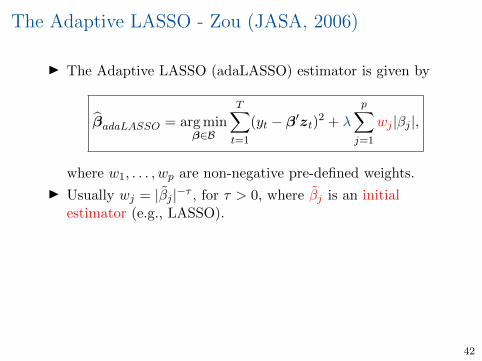
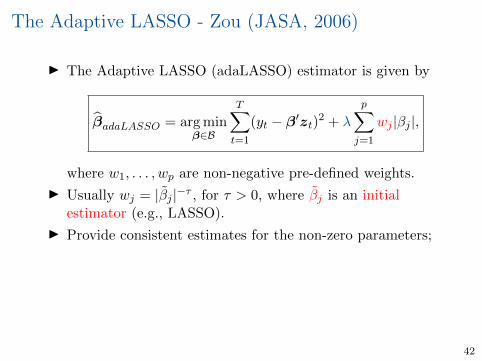
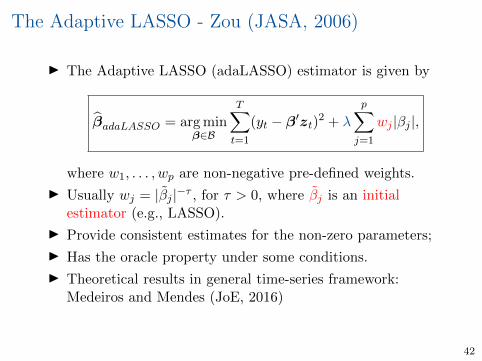
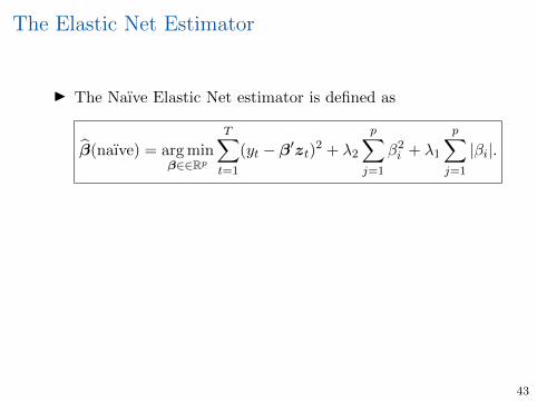
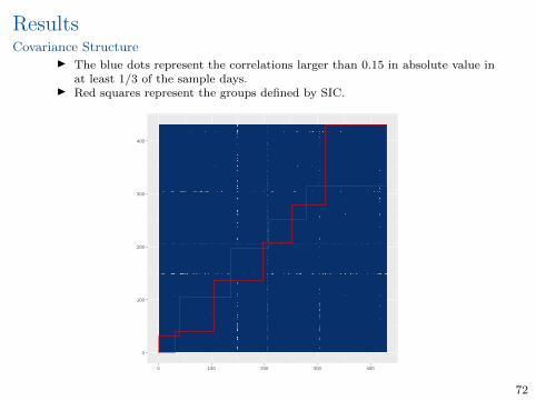
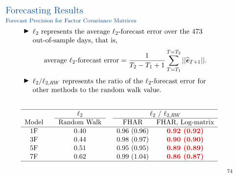
Transcript
Machine Learning Methodsin Empirical Finance
Marcelo C. Medeiros
Departamento de EconomiaPontifıcia Universidade Catolica do Rio de Janeiro
Lecture 1XVIII Encontro Brasileiro de Financas
1
Introduction
2
IWhat is Machine Learning?
– What do we want to learn?– From what do we want tolearn?
– How do we want to learn?
3
IWhat is Machine Learning?– What do we want to learn?
– From what do we want tolearn?
– How do we want to learn?
3
IWhat is Machine Learning?– What do we want to learn?– From what do we want tolearn?
– How do we want to learn?
3
IWhat is Machine Learning?– What do we want to learn?– From what do we want tolearn?
– How do we want to learn?
3
What is Machine Learning (ML)?
I Automated computer algorithms/methods +statistical models to “learn” (discover) hidden patternsfrom data.
I Usually ML methods are used for prediction (predictionanalytics) but, more recently, they are also being applied tocausal inference.
I ML methods are receiving a lot of attention ineconometrics:
– Model selection in data-rich environments (big data) forprediction and causal inference;
– Nonlinear models.
– New inferential tools (post model selection).
I When ML methods are statistically sound they arecalled Statistical Learning (SL) methods.
4
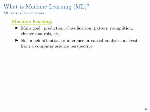
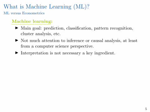
What is Machine Learning (ML)?ML versus Econometrics
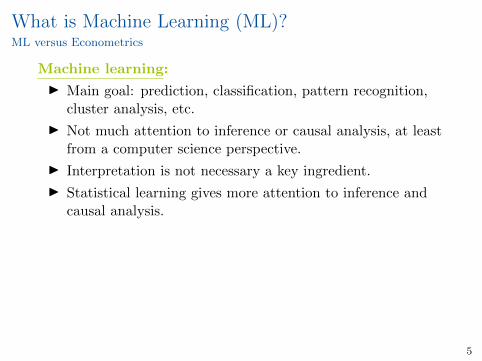
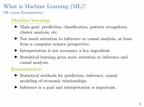
Machine learning:
I Main goal: prediction, classification, pattern recognition,cluster analysis, etc.
I Not much attention to inference or causal analysis, at leastfrom a computer science perspective.
I Interpretation is not necessary a key ingredient.
I Statistical learning gives more attention to inference andcausal analysis.
Econometrics:
I Statistical methods for prediction, inference, causalmodeling of economic relationships.
I Inference is a goal and interpretation is important.
I Causal inference is a goal for decision making.
5
What is Machine Learning (ML)?ML versus Econometrics
Machine learning:
I Main goal: prediction, classification, pattern recognition,cluster analysis, etc.
I Not much attention to inference or causal analysis, at leastfrom a computer science perspective.
I Interpretation is not necessary a key ingredient.
I Statistical learning gives more attention to inference andcausal analysis.
Econometrics:
I Statistical methods for prediction, inference, causalmodeling of economic relationships.
I Inference is a goal and interpretation is important.
I Causal inference is a goal for decision making.
5
A great matching:Machine learning
withBig Data
withEconometrics
6
A great matching:Machine learning
withBig Datawith
Econometrics
6
What is “Big Data”?
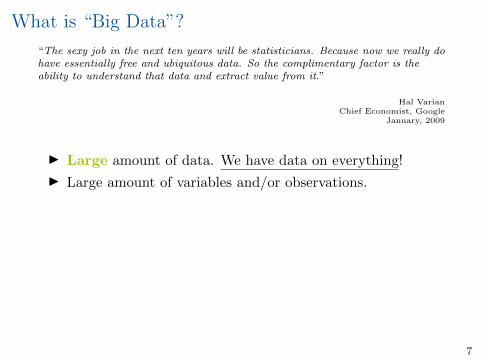
“The sexy job in the next ten years will be statisticians. Because now we really dohave essentially free and ubiquitous data. So the complimentary factor is theability to understand that data and extract value from it.”
Hal VarianChief Economist, Google
January, 2009
I Large amount of data. We have data on everything!
I Large amount of variables and/or observations.
I A quote from SAS (www.sas.comen us/insightsbig-datawhat-is-big-data.html):
“Big data is a term that describes the large volume of data – both
structured and unstructured – that inundates a business on a
day-to-day basis. But it’s not the amount of data that’s important.
It’s what organizations do with the data that matters. Big data can
be analyzed for insights that lead to better decisions and strategic
business moves.”
7
What is “Big Data”?
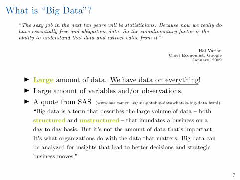
“The sexy job in the next ten years will be statisticians. Because now we really dohave essentially free and ubiquitous data. So the complimentary factor is theability to understand that data and extract value from it.”
Hal VarianChief Economist, Google
January, 2009
I Large amount of data. We have data on everything!
I Large amount of variables and/or observations.
I A quote from SAS (www.sas.comen us/insightsbig-datawhat-is-big-data.html):
“Big data is a term that describes the large volume of data – both
structured and unstructured – that inundates a business on a
day-to-day basis. But it’s not the amount of data that’s important.
It’s what organizations do with the data that matters. Big data can
be analyzed for insights that lead to better decisions and strategic
business moves.”
7
What is “Big Data”?
“The sexy job in the next ten years will be statisticians. Because now we really dohave essentially free and ubiquitous data. So the complimentary factor is theability to understand that data and extract value from it.”
Hal VarianChief Economist, Google
January, 2009
I Large amount of data. We have data on everything!
I Large amount of variables and/or observations.
I A quote from SAS (www.sas.comen us/insightsbig-datawhat-is-big-data.html):
“Big data is a term that describes the large volume of data – both
structured and unstructured – that inundates a business on a
day-to-day basis. But it’s not the amount of data that’s important.
It’s what organizations do with the data that matters. Big data can
be analyzed for insights that lead to better decisions and strategic
business moves.”
7
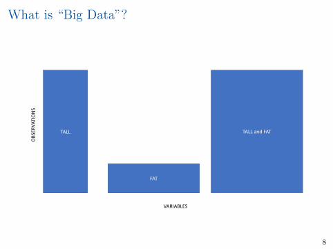
What is “Big Data”?
TALL
FAT
TALL and FAT
VARIABLES
OB
SER
VAT
ION
S
8
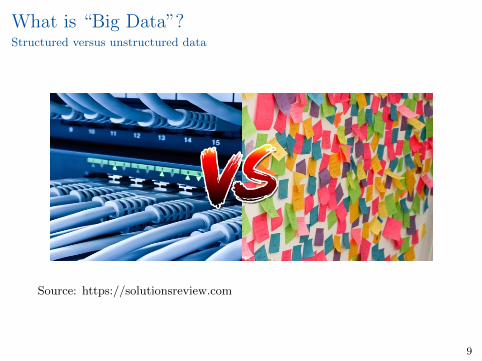
What is “Big Data”?Structured versus unstructured data
Source: https://solutionsreview.com
9
What is “Big Data”?Structured versus unstructured data
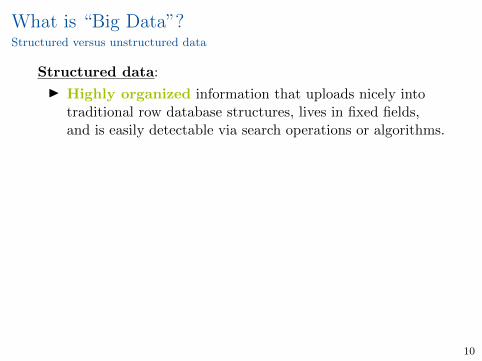
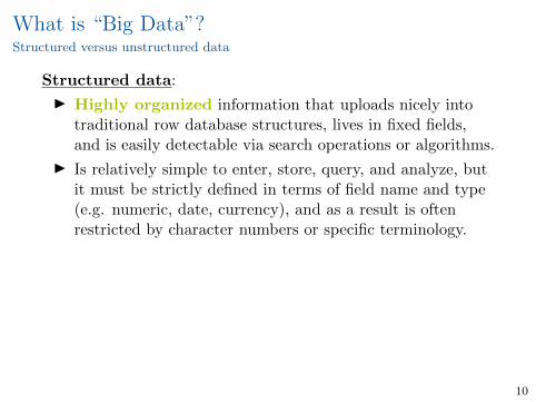
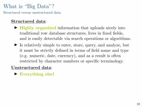
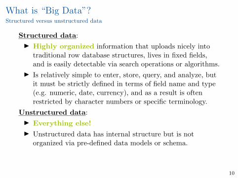
Structured data:
I Highly organized information that uploads nicely intotraditional row database structures, lives in fixed fields,and is easily detectable via search operations or algorithms.
I Is relatively simple to enter, store, query, and analyze, butit must be strictly defined in terms of field name and type(e.g. numeric, date, currency), and as a result is oftenrestricted by character numbers or specific terminology.
Unstructured data:
I Everything else!
I Unstructured data has internal structure but is notorganized via pre-defined data models or schema.
I Examples: text files, web pages, social media, email, etc...
10
What is “Big Data”?Structured versus unstructured data
Structured data:
I Highly organized information that uploads nicely intotraditional row database structures, lives in fixed fields,and is easily detectable via search operations or algorithms.
I Is relatively simple to enter, store, query, and analyze, butit must be strictly defined in terms of field name and type(e.g. numeric, date, currency), and as a result is oftenrestricted by character numbers or specific terminology.
Unstructured data:
I Everything else!
I Unstructured data has internal structure but is notorganized via pre-defined data models or schema.
I Examples: text files, web pages, social media, email, etc...
10
What is “Big Data”?From unstructured to structured data
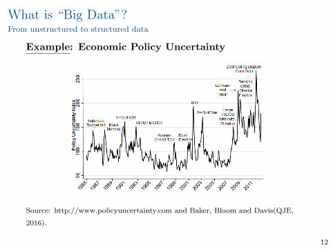
Example: Economic Policy UncertaintyBaker, Bloom and Davies (QJE, 2016)I Index from three types of underlying components:
1. First component quantifies newspaper coverage ofpolicy-related economic uncertainty.
2. A second component reflects the number of federal tax codeprovisions set to expire in future years.
3. The third component uses disagreement among economicforecasters as a proxy for uncertainty.
I From unstructured to structured data: The firstcomponent is an index of search results from 10 largenewspapers. Normalized index of the volume of newsarticles discussing economic policy uncertainty.
USA Today, the Miami Herald, the Chicago Tribune, theWashington Post, the Los Angeles Times, the Boston Globe, theSan Francisco Chronicle, the Dallas Morning News, the NewYork Times, and the Wall Street Journal.
11
What is “Big Data”?From unstructured to structured data
Example: Economic Policy Uncertainty
Source: http://www.policyuncertainty.com and Baker, Bloom and Davis(QJE,
2016).
12
What is “Big Data”?From unstructured to structured data
Example: News implied VIX (NVIX)Moreira and Manela (JFE, 2017)
I Text-based measure of uncertainty starting in 1890 usingfront-page articles of the Wall Street Journal.
I NVIX peaks during stock market crashes, times ofpolicy-related uncertainty, world wars, and financial crises.
I In US postwar data, periods when NVIX is high arefollowed by periods of above average stock returns, evenafter controlling for contemporaneous and forward-lookingmeasures of stock market volatility.
I NVIX is a key predictor of the equity premium.
I Methodology: ML regression of VIX on regressors based ontext data.
13
What is “Big Data”?From unstructured to structured data
Example: News implied VIX (NVIX)A. Manela, A. Moreira / Journal of Financial Economics 123 (2017) 137–162 141
Fig. 1. News implied volatility 1890–2009. Solid line is end-of-month Chicago Board Options Exchange volatility implied by options VIX t . Dots are news
implied volatility (NVIX), V IX t = w 0 + w · x t , where x t, i are appearances of n-gram i in month t scaled by total month t n-grams and w is estimated
with a support vector regression. The train subsample, 1996 to 2009, is used to estimate the dependency between news data and implied volatility. The
test subsample, 1986–1995, is used for out-of-sample tests of model fit. The predict subsample includes all earlier observations for which options data
and, hence, VIX are not available. Light-colored triangles indicate a nonparametric bootstrap 95% confidence interval around V IX using one thousand
randomizations. These show the sensitivity of the predicted values to randomizations of the train subsample.
Long-Term Capital Management (LTCM) crisis in August
1998, the US making clear in September 2002 that an Iraq
invasion was imminent, the abnormally low VIX from 2005
to 2007, and the financial crisis in 2008. In-sample fit is
good, with an R 2 ( train ) = 91% . The tight confidence inter-
val around ˆ v t suggests that the estimation method is not
sensitive to randomizations (with replacement) of the train
subsample. This gives us confidence that the methodology
uncovers a fairly stable mapping between word frequen-
cies and VIX, but with such a large feature space, one must
worry about over-fitting.
However, as reported in Table 1 , the model’s out-of-
sample fit over the test subsample is good, with RMSE ( test )
of 7.48 percentage points and R 2 ( test ) of 19%. In addition
to these statistics, we report results from a regression of
test subsample actual VIX values on news-based values. We
find that NVIX is a statistically powerful predictor of actual
VIX. The coefficient on ˆ v t is statistically greater than zero
( t = 4 . 01 ) and no different from one ( t = −0 . 88 ), which
supports our use of NVIX to extend VIX to the longer
sample.
2.2. NVIX is a reasonable proxy for uncertainty
NVIX captures well the fears of the average investor
over this long history. Noteworthy peaks in NVIX include
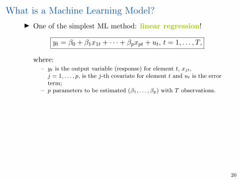
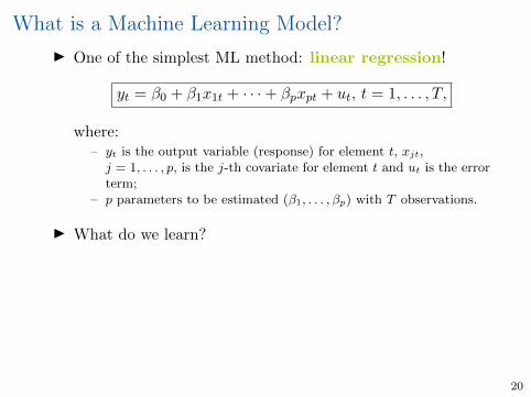
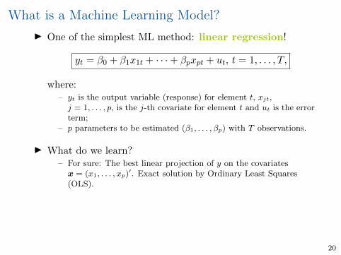
where:– yt is the output variable (response) for element t, xjt,j = 1, . . . , p, is the j-th covariate for element t and ut is the errorterm;
– p parameters to be estimated (β1, . . . , βp) with T observations.
I What do we learn?– For sure: The best linear projection of y on the covariatesx = (x1, . . . , xp)
′. Exact solution by Ordinary Least Squares(OLS).
– Under some assumptions: The E(y|x) or even the causal effectsof changes in x on y
I Linear regression is a GREAT ML method!
20
What is a Machine Learning Model?
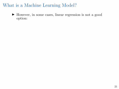
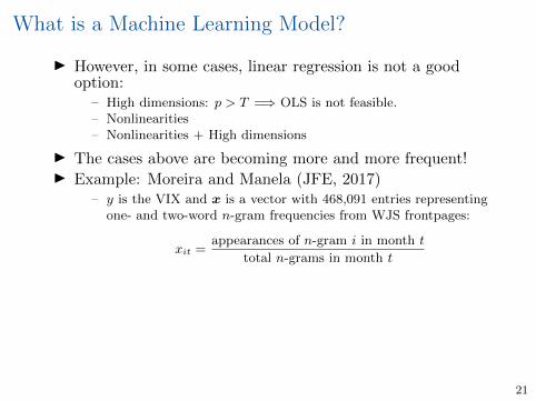
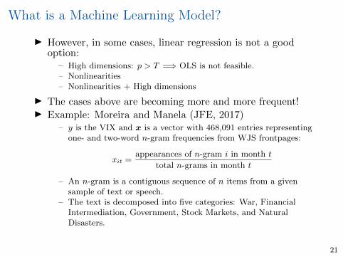
I However, in some cases, linear regression is not a goodoption:
– High dimensions: p > T =⇒ OLS is not feasible.– Nonlinearities– Nonlinearities + High dimensions
I The cases above are becoming more and more frequent!I Example: Moreira and Manela (JFE, 2017)
– y is the VIX and x is a vector with 468,091 entries representingone- and two-word n-gram frequencies from WJS frontpages:
xit =appearances of n-gram i in month t
total n-grams in month t
– An n-gram is a contiguous sequence of n items from a givensample of text or speech.
– The text is decomposed into five categories: War, FinancialIntermediation, Government, Stock Markets, and NaturalDisasters.
21
What is a Machine Learning Model?
I However, in some cases, linear regression is not a goodoption:
– High dimensions: p > T =⇒ OLS is not feasible.
– Nonlinearities– Nonlinearities + High dimensions
I The cases above are becoming more and more frequent!I Example: Moreira and Manela (JFE, 2017)
– y is the VIX and x is a vector with 468,091 entries representingone- and two-word n-gram frequencies from WJS frontpages:
xit =appearances of n-gram i in month t
total n-grams in month t
– An n-gram is a contiguous sequence of n items from a givensample of text or speech.
– The text is decomposed into five categories: War, FinancialIntermediation, Government, Stock Markets, and NaturalDisasters.
21
What is a Machine Learning Model?
I However, in some cases, linear regression is not a goodoption:
– High dimensions: p > T =⇒ OLS is not feasible.– Nonlinearities
– Nonlinearities + High dimensions
I The cases above are becoming more and more frequent!I Example: Moreira and Manela (JFE, 2017)
– y is the VIX and x is a vector with 468,091 entries representingone- and two-word n-gram frequencies from WJS frontpages:
xit =appearances of n-gram i in month t
total n-grams in month t
– An n-gram is a contiguous sequence of n items from a givensample of text or speech.
– The text is decomposed into five categories: War, FinancialIntermediation, Government, Stock Markets, and NaturalDisasters.
21
What is a Machine Learning Model?
I However, in some cases, linear regression is not a goodoption:
– High dimensions: p > T =⇒ OLS is not feasible.– Nonlinearities– Nonlinearities + High dimensions
I The cases above are becoming more and more frequent!I Example: Moreira and Manela (JFE, 2017)
– y is the VIX and x is a vector with 468,091 entries representingone- and two-word n-gram frequencies from WJS frontpages:
xit =appearances of n-gram i in month t
total n-grams in month t
– An n-gram is a contiguous sequence of n items from a givensample of text or speech.
– The text is decomposed into five categories: War, FinancialIntermediation, Government, Stock Markets, and NaturalDisasters.
21
What is a Machine Learning Model?
I However, in some cases, linear regression is not a goodoption:
– High dimensions: p > T =⇒ OLS is not feasible.– Nonlinearities– Nonlinearities + High dimensions
I The cases above are becoming more and more frequent!
I Example: Moreira and Manela (JFE, 2017)
– y is the VIX and x is a vector with 468,091 entries representingone- and two-word n-gram frequencies from WJS frontpages:
xit =appearances of n-gram i in month t
total n-grams in month t
– An n-gram is a contiguous sequence of n items from a givensample of text or speech.
– The text is decomposed into five categories: War, FinancialIntermediation, Government, Stock Markets, and NaturalDisasters.
21
What is a Machine Learning Model?
I However, in some cases, linear regression is not a goodoption:
– High dimensions: p > T =⇒ OLS is not feasible.– Nonlinearities– Nonlinearities + High dimensions
I The cases above are becoming more and more frequent!I Example: Moreira and Manela (JFE, 2017)
– y is the VIX and x is a vector with 468,091 entries representingone- and two-word n-gram frequencies from WJS frontpages:
xit =appearances of n-gram i in month t
total n-grams in month t
– An n-gram is a contiguous sequence of n items from a givensample of text or speech.
– The text is decomposed into five categories: War, FinancialIntermediation, Government, Stock Markets, and NaturalDisasters.
21
What is a Machine Learning Model?
I However, in some cases, linear regression is not a goodoption:
– High dimensions: p > T =⇒ OLS is not feasible.– Nonlinearities– Nonlinearities + High dimensions
I The cases above are becoming more and more frequent!I Example: Moreira and Manela (JFE, 2017)
– y is the VIX and x is a vector with 468,091 entries representingone- and two-word n-gram frequencies from WJS frontpages:
xit =appearances of n-gram i in month t
total n-grams in month t
– An n-gram is a contiguous sequence of n items from a givensample of text or speech.
– The text is decomposed into five categories: War, FinancialIntermediation, Government, Stock Markets, and NaturalDisasters.
21
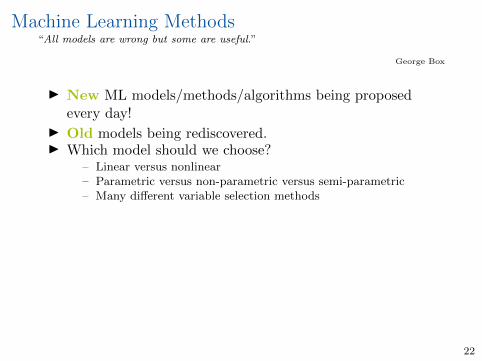
Machine Learning Methods“All models are wrong but some are useful.”
George Box
I New ML models/methods/algorithms being proposedevery day!
I Old models being rediscovered.I Which model should we choose?
– Linear versus nonlinear– Parametric versus non-parametric versus semi-parametric– Many different variable selection methods– High risk of cherry picking!!! Data-mining in the bad sense of the
– Models: linear regression, additive models, regression trees,random forests, neural networks, deep learning, kernel regression,series regression, splines.
22
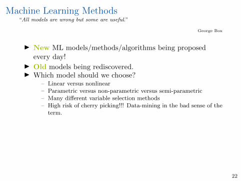
Machine Learning Methods“All models are wrong but some are useful.”
George Box
I New ML models/methods/algorithms being proposedevery day!
I Old models being rediscovered.
I Which model should we choose?
– Linear versus nonlinear– Parametric versus non-parametric versus semi-parametric– Many different variable selection methods– High risk of cherry picking!!! Data-mining in the bad sense of the
– Models: linear regression, additive models, regression trees,random forests, neural networks, deep learning, kernel regression,series regression, splines.
22
Machine Learning Methods“All models are wrong but some are useful.”
George Box
I New ML models/methods/algorithms being proposedevery day!
I Old models being rediscovered.I Which model should we choose?
– Linear versus nonlinear– Parametric versus non-parametric versus semi-parametric– Many different variable selection methods– High risk of cherry picking!!! Data-mining in the bad sense of the
– Models: linear regression, additive models, regression trees,random forests, neural networks, deep learning, kernel regression,series regression, splines.
22
Machine Learning Methods“All models are wrong but some are useful.”
George Box
I New ML models/methods/algorithms being proposedevery day!
I Old models being rediscovered.I Which model should we choose?
– Linear versus nonlinear
– Parametric versus non-parametric versus semi-parametric– Many different variable selection methods– High risk of cherry picking!!! Data-mining in the bad sense of the
– Models: linear regression, additive models, regression trees,random forests, neural networks, deep learning, kernel regression,series regression, splines.
22
Machine Learning Methods“All models are wrong but some are useful.”
George Box
I New ML models/methods/algorithms being proposedevery day!
I Old models being rediscovered.I Which model should we choose?
– Linear versus nonlinear– Parametric versus non-parametric versus semi-parametric– Many different variable selection methods– High risk of cherry picking!!! Data-mining in the bad sense of the
– Models: linear regression, additive models, regression trees,random forests, neural networks, deep learning, kernel regression,series regression, splines.
22
Machine Learning Methods“All models are wrong but some are useful.”
George Box
I New ML models/methods/algorithms being proposedevery day!
I Old models being rediscovered.I Which model should we choose?
– Linear versus nonlinear– Parametric versus non-parametric versus semi-parametric– Many different variable selection methods– High risk of cherry picking!!! Data-mining in the bad sense of the
– Models: linear regression, additive models, regression trees,random forests, neural networks, deep learning, kernel regression,series regression, splines.
22
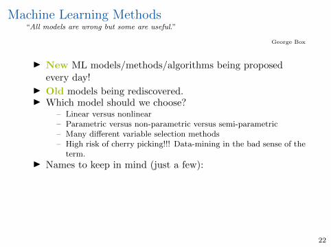
Machine Learning Methods“All models are wrong but some are useful.”
George Box
I New ML models/methods/algorithms being proposedevery day!
I Old models being rediscovered.I Which model should we choose?
– Linear versus nonlinear– Parametric versus non-parametric versus semi-parametric– Many different variable selection methods– High risk of cherry picking!!! Data-mining in the bad sense of the
term.
I Names to keep in mind (just a few):– Variable selection methods: Bagging, Boosting, LASSO,
– Models: linear regression, additive models, regression trees,random forests, neural networks, deep learning, kernel regression,series regression, splines.
22
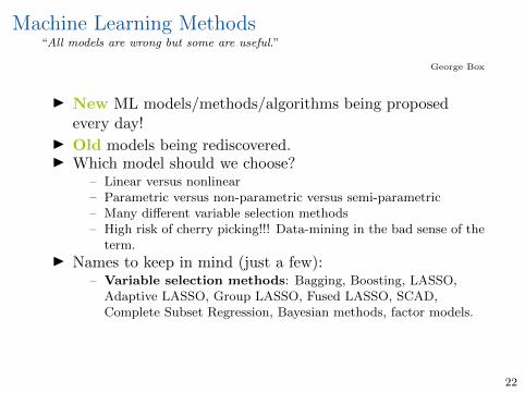
Machine Learning Methods“All models are wrong but some are useful.”
George Box
I New ML models/methods/algorithms being proposedevery day!
I Old models being rediscovered.I Which model should we choose?
– Linear versus nonlinear– Parametric versus non-parametric versus semi-parametric– Many different variable selection methods– High risk of cherry picking!!! Data-mining in the bad sense of the
term.
I Names to keep in mind (just a few):– Variable selection methods: Bagging, Boosting, LASSO,
– Models: linear regression, additive models, regression trees,random forests, neural networks, deep learning, kernel regression,series regression, splines.
22
Machine Learning Models
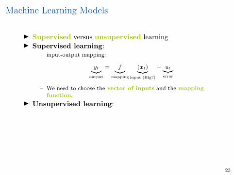
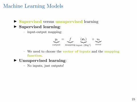
I Supervised versus unsupervised learning
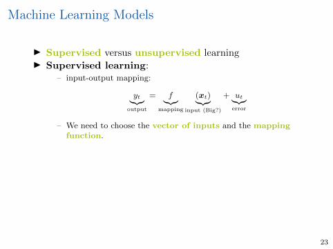
I Supervised learning:
– input-output mapping:
yt︸︷︷︸output
= f︸︷︷︸mapping
(xt)︸︷︷︸input (Big?)
+ ut︸︷︷︸error
– We need to choose the vector of inputs and the mappingfunction.
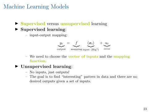
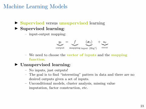
I Unsupervised learning:
– No inputs, just outputs!– The goal is to find “interesting” patters in data and there are no
desired outputs given a set of inputs.– Unconditional models, cluster analysis, missing value
imputation, factor construction, etc.
23
Machine Learning Models
I Supervised versus unsupervised learningI Supervised learning:
– input-output mapping:
yt︸︷︷︸output
= f︸︷︷︸mapping
(xt)︸︷︷︸input (Big?)
+ ut︸︷︷︸error
– We need to choose the vector of inputs and the mappingfunction.
I Unsupervised learning:– No inputs, just outputs!
– The goal is to find “interesting” patters in data and there are nodesired outputs given a set of inputs.
– Unconditional models, cluster analysis, missing valueimputation, factor construction, etc.
23
Machine Learning Models
I Supervised versus unsupervised learningI Supervised learning:
– input-output mapping:
yt︸︷︷︸output
= f︸︷︷︸mapping
(xt)︸︷︷︸input (Big?)
+ ut︸︷︷︸error
– We need to choose the vector of inputs and the mappingfunction.
I Unsupervised learning:– No inputs, just outputs!– The goal is to find “interesting” patters in data and there are no
desired outputs given a set of inputs.
– Unconditional models, cluster analysis, missing valueimputation, factor construction, etc.
23
Machine Learning Models
I Supervised versus unsupervised learningI Supervised learning:
– input-output mapping:
yt︸︷︷︸output
= f︸︷︷︸mapping
(xt)︸︷︷︸input (Big?)
+ ut︸︷︷︸error
– We need to choose the vector of inputs and the mappingfunction.
I Unsupervised learning:– No inputs, just outputs!– The goal is to find “interesting” patters in data and there are no
desired outputs given a set of inputs.– Unconditional models, cluster analysis, missing value
imputation, factor construction, etc.
23
Model SelectionI Back to the question: How should we choose a model?
– Old forecasting school: choose the model with the bestout-of-sample (OOS) performance.
– Ensamble (forecast combination): use them all.– Ensamble 2.0: use a subset of models.
I This is still an open question!I No free-lunch theorem (Wolpert, 1996): there is NO
universal best model.
– The set of assumptions that works in one domain may workpoorly in another.
I Prediction versus causality.
Big Data + Big Models + Big Set of Models
=
BIG PROBLEM!!!!
24
Model SelectionI Back to the question: How should we choose a model?
– Old forecasting school: choose the model with the bestout-of-sample (OOS) performance.
– Ensamble (forecast combination): use them all.
– Ensamble 2.0: use a subset of models.
I This is still an open question!I No free-lunch theorem (Wolpert, 1996): there is NO
universal best model.
– The set of assumptions that works in one domain may workpoorly in another.
I Prediction versus causality.
Big Data + Big Models + Big Set of Models
=
BIG PROBLEM!!!!
24
Model SelectionI Back to the question: How should we choose a model?
– Old forecasting school: choose the model with the bestout-of-sample (OOS) performance.
– Ensamble (forecast combination): use them all.– Ensamble 2.0: use a subset of models.
I This is still an open question!I No free-lunch theorem (Wolpert, 1996): there is NO
universal best model.
– The set of assumptions that works in one domain may workpoorly in another.
I Prediction versus causality.
Big Data + Big Models + Big Set of Models
=
BIG PROBLEM!!!!
24
Model SelectionI Back to the question: How should we choose a model?
– Old forecasting school: choose the model with the bestout-of-sample (OOS) performance.
– Ensamble (forecast combination): use them all.– Ensamble 2.0: use a subset of models.
I This is still an open question!
I No free-lunch theorem (Wolpert, 1996): there is NOuniversal best model.
– The set of assumptions that works in one domain may workpoorly in another.
I Prediction versus causality.
Big Data + Big Models + Big Set of Models
=
BIG PROBLEM!!!!
24
Model SelectionI Back to the question: How should we choose a model?
– Old forecasting school: choose the model with the bestout-of-sample (OOS) performance.
– Ensamble (forecast combination): use them all.– Ensamble 2.0: use a subset of models.
I This is still an open question!I No free-lunch theorem (Wolpert, 1996): there is NO
universal best model.
– The set of assumptions that works in one domain may workpoorly in another.
I Prediction versus causality.
Big Data + Big Models + Big Set of Models
=
BIG PROBLEM!!!!
24
Model SelectionI Back to the question: How should we choose a model?
– Old forecasting school: choose the model with the bestout-of-sample (OOS) performance.
– Ensamble (forecast combination): use them all.– Ensamble 2.0: use a subset of models.
I This is still an open question!I No free-lunch theorem (Wolpert, 1996): there is NO
universal best model.– The set of assumptions that works in one domain may work
poorly in another.
I Prediction versus causality.
Big Data + Big Models + Big Set of Models
=
BIG PROBLEM!!!!
24
Prediction and Inference after Model SelectionI Conducting inference with respect a set of parameters after
model selection is a challenging task.
I Finite sample inference is very complicated and theasymptotic results are usually not uniform over a wideclass of probability distributions ⇒ asymptoticdistributions depend on the values of the true parameter.
I Difficult to distinguish among smallish coefficients and zero.I Inferential procedures must be adapted and conducting
standard test ignoring model selection is wrong. Solutionavailable for cross-section (see Victor Chernozhukov’spapers). For time-series, solutions available only for specificsettings; see Carvalho, Masini and Medeiros (JoE, in press).
I The lack of uniform convergence is not a problem of BigData (high-dimensions) and it is due to the model searchmethods that are applied before inference is conducted.
I On the other hand, prediction (forecasting) after modelselection is a much easier task.
25
Prediction and Inference after Model SelectionI Conducting inference with respect a set of parameters after
model selection is a challenging task.I Finite sample inference is very complicated and the
asymptotic results are usually not uniform over a wideclass of probability distributions ⇒ asymptoticdistributions depend on the values of the true parameter.
I Difficult to distinguish among smallish coefficients and zero.
I Inferential procedures must be adapted and conductingstandard test ignoring model selection is wrong. Solutionavailable for cross-section (see Victor Chernozhukov’spapers). For time-series, solutions available only for specificsettings; see Carvalho, Masini and Medeiros (JoE, in press).
I The lack of uniform convergence is not a problem of BigData (high-dimensions) and it is due to the model searchmethods that are applied before inference is conducted.
I On the other hand, prediction (forecasting) after modelselection is a much easier task.
25
Prediction and Inference after Model SelectionI Conducting inference with respect a set of parameters after
model selection is a challenging task.I Finite sample inference is very complicated and the
asymptotic results are usually not uniform over a wideclass of probability distributions ⇒ asymptoticdistributions depend on the values of the true parameter.
I Difficult to distinguish among smallish coefficients and zero.I Inferential procedures must be adapted and conducting
standard test ignoring model selection is wrong. Solutionavailable for cross-section (see Victor Chernozhukov’spapers). For time-series, solutions available only for specificsettings; see Carvalho, Masini and Medeiros (JoE, in press).
I The lack of uniform convergence is not a problem of BigData (high-dimensions) and it is due to the model searchmethods that are applied before inference is conducted.
I On the other hand, prediction (forecasting) after modelselection is a much easier task.
25
Prediction and Inference after Model SelectionI Conducting inference with respect a set of parameters after
model selection is a challenging task.I Finite sample inference is very complicated and the
asymptotic results are usually not uniform over a wideclass of probability distributions ⇒ asymptoticdistributions depend on the values of the true parameter.
I Difficult to distinguish among smallish coefficients and zero.I Inferential procedures must be adapted and conducting
standard test ignoring model selection is wrong. Solutionavailable for cross-section (see Victor Chernozhukov’spapers). For time-series, solutions available only for specificsettings; see Carvalho, Masini and Medeiros (JoE, in press).
I The lack of uniform convergence is not a problem of BigData (high-dimensions) and it is due to the model searchmethods that are applied before inference is conducted.
I On the other hand, prediction (forecasting) after modelselection is a much easier task.
25
Model Selection in High-Dimensions
I High-Dimensional Models:
– Relatively High-Dimension: Models with many candidatevariables p compared to the sample size n (or T ), but usuallyless than n.
– Moderately High-Dimension: Models with candidatevariables proportional to the sample size, usually greater thanthe sample size.
– High-Dimension: Models with more candidate variables thanobservations, and the number of candidate variables growspolynomially or exponentially with n (or T ).
26
Model Selection in High-Dimensions: Challenges
1. Prediction, oracle properties.Same prediction performance as the “true” model.
2. Variable (Model) selection.Select only the correct set of relevant variables.
3. Variable screening.Select at least the correct set of variables.
4. Inference.Distribution of the estimates.
27
Model Selection in High-Dimensions
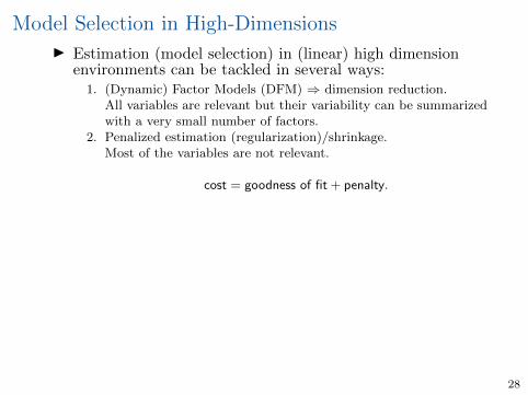
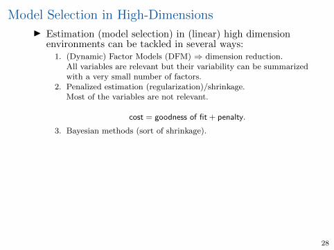
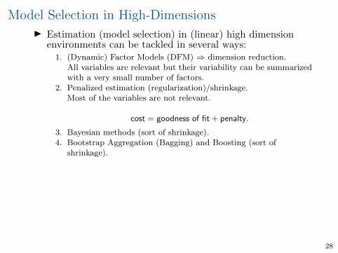
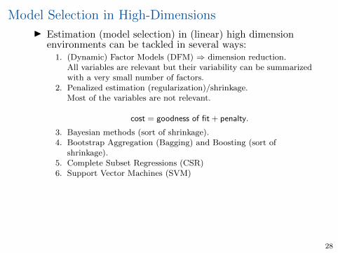
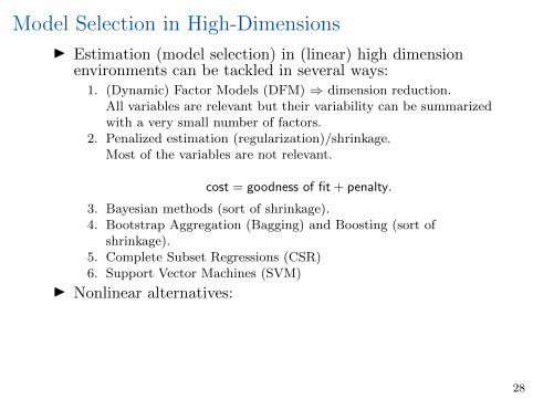
I Estimation (model selection) in (linear) high dimensionenvironments can be tackled in several ways:
1. (Dynamic) Factor Models (DFM) ⇒ dimension reduction.All variables are relevant but their variability can be summarizedwith a very small number of factors.
2. Penalized estimation (regularization)/shrinkage.Most of the variables are not relevant.
cost = goodness of fit + penalty.
3. Bayesian methods (sort of shrinkage).4. Bootstrap Aggregation (Bagging) and Boosting (sort of
shrinkage).5. Complete Subset Regressions (CSR)6. Support Vector Machines (SVM)
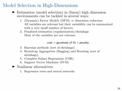
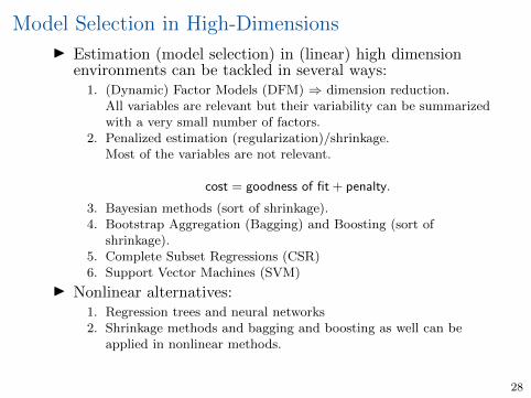
I Nonlinear alternatives:
1. Regression trees and neural networks2. Shrinkage methods and bagging and boosting as well can be
applied in nonlinear methods.3. Bayesian methods.
28
Model Selection in High-Dimensions
I Estimation (model selection) in (linear) high dimensionenvironments can be tackled in several ways:
1. (Dynamic) Factor Models (DFM) ⇒ dimension reduction.All variables are relevant but their variability can be summarizedwith a very small number of factors.
2. Penalized estimation (regularization)/shrinkage.Most of the variables are not relevant.
cost = goodness of fit + penalty.
3. Bayesian methods (sort of shrinkage).4. Bootstrap Aggregation (Bagging) and Boosting (sort of
shrinkage).5. Complete Subset Regressions (CSR)6. Support Vector Machines (SVM)
I Nonlinear alternatives:
1. Regression trees and neural networks2. Shrinkage methods and bagging and boosting as well can be
applied in nonlinear methods.3. Bayesian methods.
28
Model Selection in High-Dimensions
I Estimation (model selection) in (linear) high dimensionenvironments can be tackled in several ways:
1. (Dynamic) Factor Models (DFM) ⇒ dimension reduction.All variables are relevant but their variability can be summarizedwith a very small number of factors.
2. Penalized estimation (regularization)/shrinkage.Most of the variables are not relevant.
cost = goodness of fit + penalty.
3. Bayesian methods (sort of shrinkage).
4. Bootstrap Aggregation (Bagging) and Boosting (sort ofshrinkage).
5. Complete Subset Regressions (CSR)6. Support Vector Machines (SVM)
I Nonlinear alternatives:
1. Regression trees and neural networks2. Shrinkage methods and bagging and boosting as well can be
applied in nonlinear methods.3. Bayesian methods.
28
Model Selection in High-Dimensions
I Estimation (model selection) in (linear) high dimensionenvironments can be tackled in several ways:
1. (Dynamic) Factor Models (DFM) ⇒ dimension reduction.All variables are relevant but their variability can be summarizedwith a very small number of factors.
2. Penalized estimation (regularization)/shrinkage.Most of the variables are not relevant.
cost = goodness of fit + penalty.
3. Bayesian methods (sort of shrinkage).4. Bootstrap Aggregation (Bagging) and Boosting (sort of
shrinkage).
5. Complete Subset Regressions (CSR)6. Support Vector Machines (SVM)
I Nonlinear alternatives:
1. Regression trees and neural networks2. Shrinkage methods and bagging and boosting as well can be
applied in nonlinear methods.3. Bayesian methods.
28
Model Selection in High-Dimensions
I Estimation (model selection) in (linear) high dimensionenvironments can be tackled in several ways:
1. (Dynamic) Factor Models (DFM) ⇒ dimension reduction.All variables are relevant but their variability can be summarizedwith a very small number of factors.
2. Penalized estimation (regularization)/shrinkage.Most of the variables are not relevant.
cost = goodness of fit + penalty.
3. Bayesian methods (sort of shrinkage).4. Bootstrap Aggregation (Bagging) and Boosting (sort of
shrinkage).5. Complete Subset Regressions (CSR)
6. Support Vector Machines (SVM)
I Nonlinear alternatives:
1. Regression trees and neural networks2. Shrinkage methods and bagging and boosting as well can be
applied in nonlinear methods.3. Bayesian methods.
28
Model Selection in High-Dimensions
I Estimation (model selection) in (linear) high dimensionenvironments can be tackled in several ways:
1. (Dynamic) Factor Models (DFM) ⇒ dimension reduction.All variables are relevant but their variability can be summarizedwith a very small number of factors.
2. Penalized estimation (regularization)/shrinkage.Most of the variables are not relevant.
cost = goodness of fit + penalty.
3. Bayesian methods (sort of shrinkage).4. Bootstrap Aggregation (Bagging) and Boosting (sort of
shrinkage).5. Complete Subset Regressions (CSR)6. Support Vector Machines (SVM)
I Nonlinear alternatives:
1. Regression trees and neural networks2. Shrinkage methods and bagging and boosting as well can be
applied in nonlinear methods.3. Bayesian methods.
28
Model Selection in High-Dimensions
I Estimation (model selection) in (linear) high dimensionenvironments can be tackled in several ways:
1. (Dynamic) Factor Models (DFM) ⇒ dimension reduction.All variables are relevant but their variability can be summarizedwith a very small number of factors.
2. Penalized estimation (regularization)/shrinkage.Most of the variables are not relevant.
cost = goodness of fit + penalty.
3. Bayesian methods (sort of shrinkage).4. Bootstrap Aggregation (Bagging) and Boosting (sort of
shrinkage).5. Complete Subset Regressions (CSR)6. Support Vector Machines (SVM)
I Nonlinear alternatives:1. Regression trees and neural networks
2. Shrinkage methods and bagging and boosting as well can beapplied in nonlinear methods.
3. Bayesian methods.
28
Model Selection in High-Dimensions
I Estimation (model selection) in (linear) high dimensionenvironments can be tackled in several ways:
1. (Dynamic) Factor Models (DFM) ⇒ dimension reduction.All variables are relevant but their variability can be summarizedwith a very small number of factors.
2. Penalized estimation (regularization)/shrinkage.Most of the variables are not relevant.
cost = goodness of fit + penalty.
3. Bayesian methods (sort of shrinkage).4. Bootstrap Aggregation (Bagging) and Boosting (sort of
shrinkage).5. Complete Subset Regressions (CSR)6. Support Vector Machines (SVM)
I Nonlinear alternatives:1. Regression trees and neural networks2. Shrinkage methods and bagging and boosting as well can be
applied in nonlinear methods.
3. Bayesian methods.
28
Model Selection in High-Dimensions
I Estimation (model selection) in (linear) high dimensionenvironments can be tackled in several ways:
1. (Dynamic) Factor Models (DFM) ⇒ dimension reduction.All variables are relevant but their variability can be summarizedwith a very small number of factors.
2. Penalized estimation (regularization)/shrinkage.Most of the variables are not relevant.
cost = goodness of fit + penalty.
3. Bayesian methods (sort of shrinkage).4. Bootstrap Aggregation (Bagging) and Boosting (sort of
shrinkage).5. Complete Subset Regressions (CSR)6. Support Vector Machines (SVM)
I Nonlinear alternatives:1. Regression trees and neural networks2. Shrinkage methods and bagging and boosting as well can be
applied in nonlinear methods.3. Bayesian methods.
28
The Road Map
Lecture 1:
I Linear models with shrinkage
I Applications to covariance matrix forecasting
Lecture 2:
I Nonlinear models
I Applications to equity premium forecasting
29
Shrinkage in Linear Models:Ridge, LASSO, Adaptive LASSO, Elastic
NetWhat happens when p >> T in linear regressions?
30
Framework: Linear Regression Model
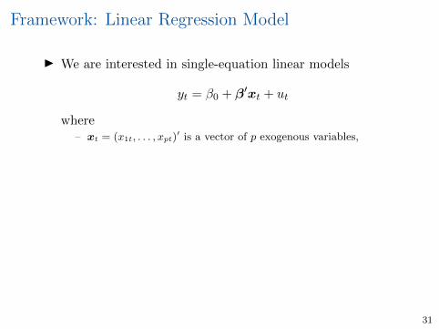
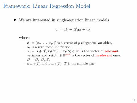
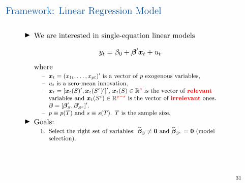
I We are interested in single-equation linear models
yt = β0 + β′xt + ut
where
– xt = (x1t, . . . , xpt)′ is a vector of p exogenous variables,
– ut is a zero-mean innovation,– xt = [xt(S)′,xt(S
c)′]′, xt(S) ∈ Rs is the vector of relevantvariables and xt(S
c) ∈ Rp−s is the vector of irrelevant ones.β = [β′S ,β
′Sc ]′.
– p ≡ p(T ) and s ≡ s(T ). T is the sample size.
I Goals:
1. Select the right set of variables: βS 6= 0 and βSc = 0 (modelselection).
2. Estimate βS as if the correct set of variables is known to theeconometrician.
31
Framework: Linear Regression Model
I We are interested in single-equation linear models
yt = β0 + β′xt + ut
where– xt = (x1t, . . . , xpt)
′ is a vector of p exogenous variables,
– ut is a zero-mean innovation,– xt = [xt(S)′,xt(S
c)′]′, xt(S) ∈ Rs is the vector of relevantvariables and xt(S
c) ∈ Rp−s is the vector of irrelevant ones.β = [β′S ,β
′Sc ]′.
– p ≡ p(T ) and s ≡ s(T ). T is the sample size.
I Goals:
1. Select the right set of variables: βS 6= 0 and βSc = 0 (modelselection).
2. Estimate βS as if the correct set of variables is known to theeconometrician.
31
Framework: Linear Regression Model
I We are interested in single-equation linear models
yt = β0 + β′xt + ut
where– xt = (x1t, . . . , xpt)
′ is a vector of p exogenous variables,– ut is a zero-mean innovation,
– xt = [xt(S)′,xt(Sc)′]′, xt(S) ∈ Rs is the vector of relevant
variables and xt(Sc) ∈ Rp−s is the vector of irrelevant ones.
β = [β′S ,β′Sc ]′.
– p ≡ p(T ) and s ≡ s(T ). T is the sample size.
I Goals:
1. Select the right set of variables: βS 6= 0 and βSc = 0 (modelselection).
2. Estimate βS as if the correct set of variables is known to theeconometrician.
31
Framework: Linear Regression Model
I We are interested in single-equation linear models
yt = β0 + β′xt + ut
where– xt = (x1t, . . . , xpt)
′ is a vector of p exogenous variables,– ut is a zero-mean innovation,– xt = [xt(S)′,xt(S
c)′]′, xt(S) ∈ Rs is the vector of relevantvariables and xt(S
c) ∈ Rp−s is the vector of irrelevant ones.β = [β′S ,β
′Sc ]′.
– p ≡ p(T ) and s ≡ s(T ). T is the sample size.
I Goals:
1. Select the right set of variables: βS 6= 0 and βSc = 0 (modelselection).
2. Estimate βS as if the correct set of variables is known to theeconometrician.
31
Framework: Linear Regression Model
I We are interested in single-equation linear models
yt = β0 + β′xt + ut
where– xt = (x1t, . . . , xpt)
′ is a vector of p exogenous variables,– ut is a zero-mean innovation,– xt = [xt(S)′,xt(S
c)′]′, xt(S) ∈ Rs is the vector of relevantvariables and xt(S
c) ∈ Rp−s is the vector of irrelevant ones.β = [β′S ,β
′Sc ]′.
– p ≡ p(T ) and s ≡ s(T ). T is the sample size.
I Goals:1. Select the right set of variables: βS 6= 0 and βSc = 0 (model
selection).
2. Estimate βS as if the correct set of variables is known to theeconometrician.
31
Framework: Linear Regression Model
I We are interested in single-equation linear models
yt = β0 + β′xt + ut
where– xt = (x1t, . . . , xpt)
′ is a vector of p exogenous variables,– ut is a zero-mean innovation,– xt = [xt(S)′,xt(S
c)′]′, xt(S) ∈ Rs is the vector of relevantvariables and xt(S
c) ∈ Rp−s is the vector of irrelevant ones.β = [β′S ,β
′Sc ]′.
– p ≡ p(T ) and s ≡ s(T ). T is the sample size.
I Goals:1. Select the right set of variables: βS 6= 0 and βSc = 0 (model
selection).2. Estimate βS as if the correct set of variables is known to the
econometrician.
31
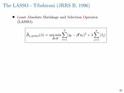
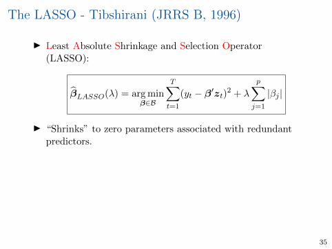
Penalized Least Squares
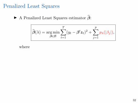
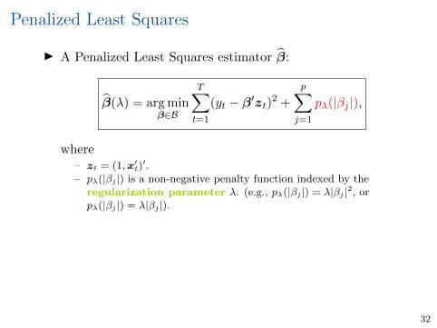
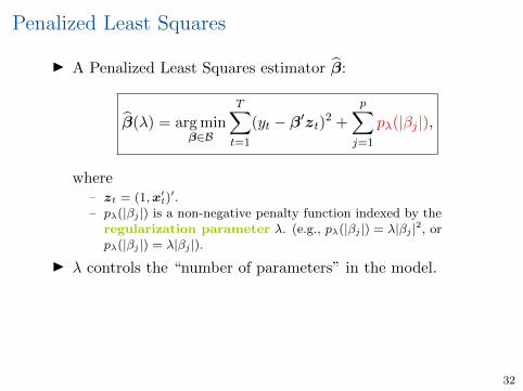
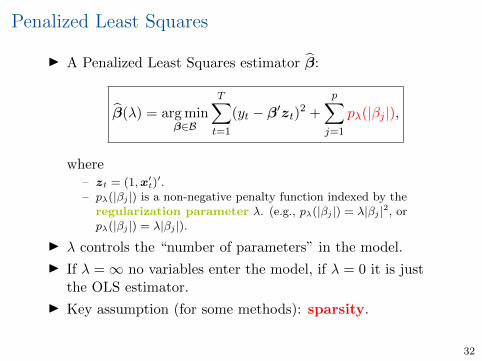
I A Penalized Least Squares estimator β:
β(λ) = arg minβ∈B
T∑t=1
(yt − β′zt)2 +
p∑j=1
pλ(|βj |),
where
– zt = (1,x′t)′.
– pλ(|βj |) is a non-negative penalty function indexed by theregularization parameter λ. (e.g., pλ(|βj |) = λ|βj |2, orpλ(|βj |) = λ|βj |).
I λ controls the “number of parameters” in the model.
I If λ =∞ no variables enter the model, if λ = 0 it is justthe OLS estimator.
I Key assumption (for some methods): sparsity.
32
Penalized Least Squares
I A Penalized Least Squares estimator β:
β(λ) = arg minβ∈B
T∑t=1
(yt − β′zt)2 +
p∑j=1
pλ(|βj |),
where– zt = (1,x′t)
′.
– pλ(|βj |) is a non-negative penalty function indexed by theregularization parameter λ. (e.g., pλ(|βj |) = λ|βj |2, orpλ(|βj |) = λ|βj |).
I λ controls the “number of parameters” in the model.
I If λ =∞ no variables enter the model, if λ = 0 it is justthe OLS estimator.
I Key assumption (for some methods): sparsity.
32
Penalized Least Squares
I A Penalized Least Squares estimator β:
β(λ) = arg minβ∈B
T∑t=1
(yt − β′zt)2 +
p∑j=1
pλ(|βj |),
where– zt = (1,x′t)
′.– pλ(|βj |) is a non-negative penalty function indexed by the
I λ controls the “number of parameters” in the model.
I If λ =∞ no variables enter the model, if λ = 0 it is justthe OLS estimator.
I Key assumption (for some methods): sparsity.
32
Sparse Models
I We say a model is sparse if the true parameter vector β issparse, i.e., most elements in β are either zero ornegligibly small (compared to the sample size).
I In some cases (for example, linear models for theconditional mean) it is equivalent to say that the numberof relevant variables is small compared to the number ofcandidate variables.
I Sparse modeling has been successfully used to deal withhigh-dimensional models and is a crucial condition foridentifiability.
33
The Ridge Regression
I The Ridge estimator is defined as follows:
βRidge(λ) = arg minβ∈B
T∑t=1
(yt − β′zt)2 + λ
p∑j=0
β2j
I “Shrinks” towards zero parameters associated withredundant predictors (not exactly).
I λ is a shrinkage parameter to be chosen;
I The Ridge solution is not sparse.
I The solution βRidge is easy to find as the problem remainsquadratic in β:
βRidge (λ) =(Z ′Z + λI
)−1Z ′y.
I Good for prediction but not for variable selection.
34
The LASSO - Tibshirani (JRRS B, 1996)
I Least Absolute Shrinkage and Selection Operator(LASSO):
βLASSO(λ) = arg minβ∈B
T∑t=1
(yt − β′zt)2 + λ
p∑j=1
|βj |
I “Shrinks” to zero parameters associated with redundantpredictors.
I The regularization path can be efficiently estimated.
I Can handle (many) more variables than observations(p >> T ).
I Under some conditions can select the correct subset ofrelevant variables.
35
LASSO versus Ridge
7
Picture of Lasso and Ridge regression
β^ β^2. .β
1
β2
β1β
36
LASSO and Model SelectionConsistency
Estimation Consistency
β − β0 p−→ 0, asT −→∞.
Model Selection Consistency
P
({i : β 6= 0
}={i : β0 6= 0
})−→ 1, asT −→∞.
Sign Consistency
P(β
s= β0
)−→ 1 asT −→∞
whereβ
s= β0 ⇐⇒ sign
(β)
= sign(β0)
37
LASSO and Model SelectionThe sign Function
The sign function is defined as
sign(x) =
1 ifx > 0
0 ifx = 0
−1 ifx < 0
38
Sign ConsistencyDefinitions
Strong Sign Consistency
The LASSO estimator is strongly sign consistent if∃λT = f(T ) such that
limT→∞
P(β(λT )
s= β0
)= 1
General Sign Consistency
The LASSO estimator is general sign consistent if
limT→∞
P(∃λ, β(λ)
s= β0
)= 1
I Strong sign consistency implies general sign consistency
39
LASSO and Model SelectionSign Consistency
General Sign Consistency versus Strong Sign Consistency
I Strong Sign Consistency implies one can use apre-selected λ to achieve consistent model selection via theLASSO.
I General Sign Consistency means for a randomrealization there exists a correct amount of regularizationthat selects the true model.
40
LASSO and Model SelectionIrrepresentable Condition
Strong Irrepresentable Condition
∃η > 0 such that ∣∣∣∣ΣScSΣ−1
SSsign(β0S
)∣∣∣∣ ≤ 1− η
Weak Irrepresentable Condition∣∣∣∣ΣScSΣ−1
SSsign(β0S
)∣∣∣∣ < 1
I 1 ∈ R(p−s) is a vector of ones, and the inequality holdselement-wise.
I The Irrepresentable Condition is a key condition for modelselection consistency of the LASSO!
I This is a too strong condition!
41
LASSO and Model SelectionIrrepresentable Condition
Strong Irrepresentable Condition
∃η > 0 such that ∣∣∣∣ΣScSΣ−1
SSsign(β0S
)∣∣∣∣ ≤ 1− η
Weak Irrepresentable Condition∣∣∣∣ΣScSΣ−1
SSsign(β0S
)∣∣∣∣ < 1
I 1 ∈ R(p−s) is a vector of ones, and the inequality holdselement-wise.
I The Irrepresentable Condition is a key condition for modelselection consistency of the LASSO!
I This is a too strong condition! 41
The Adaptive LASSO - Zou (JASA, 2006)
I The Adaptive LASSO (adaLASSO) estimator is given by
βadaLASSO = arg minβ∈B
T∑t=1
(yt − β′zt)2 + λ
p∑j=1
wj |βj |,
where w1, . . . , wp are non-negative pre-defined weights.
I Usually wj = |βj |−τ , for τ > 0, where βj is an initialestimator (e.g., LASSO).
I Provide consistent estimates for the non-zero parameters;
I Has the oracle property under some conditions.
I Theoretical results in general time-series framework:Medeiros and Mendes (JoE, 2016)
42
The Elastic Net Estimator
I The Naıve Elastic Net estimator is defined as
β(naıve) = arg minβ∈∈Rp
T∑t=1
(yt − β′zt)2 + λ2
p∑j=1
β2i + λ1
p∑j=1
|βi|.
I The Elastic Net estimator is given by
β = (1 + λ2)β(naıve).
I The naıve EL-Net estimator selects the same model as theEL-Net version.
43
The Elastic Net Estimator
I The Naıve Elastic Net estimator is defined as
β(naıve) = arg minβ∈∈Rp
T∑t=1
(yt − β′zt)2 + λ2
p∑j=1
β2i + λ1
p∑j=1
|βi|.
I The Elastic Net estimator is given by
β = (1 + λ2)β(naıve).
I The naıve EL-Net estimator selects the same model as theEL-Net version.
43
The Elastic Net Estimator
I The Naıve Elastic Net estimator is defined as
β(naıve) = arg minβ∈∈Rp
T∑t=1
(yt − β′zt)2 + λ2
p∑j=1
β2i + λ1
p∑j=1
|βi|.
I The Elastic Net estimator is given by
β = (1 + λ2)β(naıve).
I The naıve EL-Net estimator selects the same model as theEL-Net version.
43
The Elastic Net EstimatorThe Geometry of the Elastic Net
ElasticNet Hui Zou, Stanford University 10
Geometry of the elastic net
β1
β2
RidgeLassoElastic Net
2-dimensional illustration α = 0.5
The elastic net penalty
J(β) = α‖β‖2+(1−α)‖β‖1
(with α = λ2
λ2+λ1)
minβ
‖y−Xβ‖2 s.t. J(β) ≤ t.
• Singularities at the
vertexes (necessary for
sparsity)
• Strict convex edges.
The strength of con-
vexity varies with α
(grouping)
44
To Learn More about Shrinkage
45
Empirical Example:Forecasting Large Dimensional Realized
Covariance Matrices
Callot, Laurent, Anders B. Kock and Marcelo C. Medeiros (2017). Modeling and
Forecasting Large Realized Covariance Matrices and Portfolio Choice. Journal
of Applied Econometrics, 32, 140-158.
46
Dataset
I 30 stocks from the Dow Jones index from 2006 to 2012with a total of 1474 daily observations.
I Daily realized covariances are constructed from 5 minutesreturns by the method of Lunde, Shephard, Sheppard(2013).
I The stocks can be classified in 8 broad categories.
where:– f1,t, · · · , fK,t are the excess returns of K factors;– βik,t, k = 1, . . . ,K, are factor loadings for asset i;– εi,t is the idiosyncratic error term.
I Factors are linear combinations of returns: long-short stockportfolios where stocks are sorted on firm characteristics:
I The dynamics for ysε,t = vech[logM(Σsε,t)],s ∈ {1, 2, . . . , S}:
ysε,t = ωsε + ΦsΛsε,t−1 + usε,t,
where Λsε,t−1 = diag[logM(Σs
ε,t−1)].
I LASSO/adaLASSO estimation equation by equation.
68
DataRealized Covariance Matrices
I The data consists of daily realized covariance matrices ofreturns for constituents of the S&P 500 index
I We consider companies that remained in the index and hadbalance sheet data for the full sample period, totaling 430stocks
I These matrices were constructed from 5-minute returns bycomposite realized kernel (Lunde et al, 2016 JBES)
I Sample period: January 2006 - December 2011 (1495 days).Estimation windows with 1,000 observations.
I Data cleaning: merges and splits.
69
DataFactors and Sector Classification
I 6 factors + market are considered: Size (SMB), Value(HML), Gross Profitability, Investment, Asset Growth andAccruals (CRSP/Compustat database)
I 4 different combinations: 1F(Market), 3F(1F + Sizeand Value), 5F(3F + Gross Profitability and Investment),and 7F(5F + Asset Growth and Accruals)
I Standard Industrial Classification (SIC): 10 sectors
70
DataNumber of Stocks per Sector
Sector Number of Stocks
Consumer Non-Durables 31Consumer Durables 8Manufacturing 65Oil, Gas, and Coal Extraction 32Business Equipment 61Telecommunications 10Wholesale and Retail 45Health Care, Medical Equipments, and Drugs 26Utilities 36Others 116
71
ResultsCovariance Structure
I The blue dots represent the correlations larger than 0.15 in absolute value inat least 1/3 of the sample days.
I Red squares represent the groups defined by SIC.
0
100
200
300
400
0 100 200 300 400
72
ResultsFactor Decomposition and Residual Covariance
73
Forecasting ResultsForecast Precision for Factor Covariance Matrices
I `2 represents the average `2-forecast error over the 473out-of-sample days, that is,
average `2-forecast error =1
T2 − T1 + 1
T=T2∑T=T1
||εT+1||.
I `2/`2,RW represents the ratio of the `2-forecast error forother methods to the random walk value.
`2 `2 / `2,RWModel Random Walk FHAR FHAR, Log-matrix