92
Machine learning solutions to visual recognition problems Jakob Verbeek Synth` ese des travaux scientifiques pour obtenir le grade de Habilitation ` a Diriger des Recherches.

Machine learning solutionsto visual recognition problems
Jakob Verbeek
Synthese des travaux scientifiques pour obtenir le grade deHabilitation a Diriger des Recherches.
Summary
This thesis gives an overview of my research since my arrival in December2005 as a postdoctoral fellow at the in the LEAR team at INRIA Rhone-Alpes. After a general introduction in Chapter 1, the contributions are pre-sented in chapters 2–4 along three themes. In each chapter we describe thecontributions, their relation to related work, and highlight two contribu-tions with more detail.
Chapter 2 is concerned with contributions related to the Fisher vec-tor representation. We highlight an extension of the representation basedon modeling dependencies among local descriptors (Cinbis et al., 2012,2016a). The second highlight is on an approximate normalization schemewhich speeds-up applications for object and action localization (Oneataet al., 2014b).
In Chapter 3 we consider the contributions related to metric learning.The first contribution we highlight is a nearest-neighbor based image an-notation method that learns weights over neighbors, and effectively de-termines the number of neighbors to use (Guillaumin et al., 2009a). Thesecond contribution we highlight is an image classification method basedon metric learning for the nearest class mean classifier that can efficientlygeneralize to new classes (Mensink et al., 2012, 2013b).
The third set of contributions, presented in Chapter 4, is related to learn-ing visual recognition models from incomplete supervision. The first high-lighted contribution is an interactive image annotation method that ex-ploits dependencies across different image labels, to improve predictionsand to identify the most informative user input (Mensink et al., 2011, 2013a).The second highlighted contribution is a multi-fold multiple instance learn-ing method for learning object localization models from training imageswhere we only know if the object is present in the image or not (Cinbiset al., 2014, 2016b).
Finally, Chapter 5 summarizes the contributions, and presents future re-search directions. A curriculum vitae with a list of publications is availablein Appendix A.
i

Resume
Cette these donne un apercu de mes recherches depuis mon arrivee endecembre 2005 en tant que postdoctorat au sein de l’equipe LEAR a l’INRIARhone-Alpes. Apres une introduction generale au Chapitre 1, les contribu-tions seront presentees dans les chapitres 2–4. Chaque chapitre decrira lescontributions lies a un theme et leur relation avec les travaux y afferent.Deux contributions seront egalement mise en exergue.
Le Chapitre 2 concernera les contributions liees a la representation vec-torielle de Fisher. Nous mettons en avant une extension de cette representa-tion basee sur la modelisation des dependances parmi les descripteurs lo-caux (Cinbis et al., 2012, 2016a). La deuxieme contribution presentee endetail est un ensemble d’approximations des normalisations du vecteur deFisher, qui permettent une acceleration dans des applications de localisa-tion d’objets et d’actions (Oneata et al., 2014b).
Dans le Chapitre 3, nous considererons les contributions liees a l’ap-prentissage de metrique. La premiere contribution que nous detailleronsest une methode d’annotation d’image type plus proche voisin. Cette meth-ode permet d’affecter des poids aux voisins et de determiner le nombre devoisins a utiliser (Guillaumin et al., 2009a). La deuxieme contribution quenous mettrons en valeur est une methode de classification d’image baseesur l’apprentissage de metrique qui permet de generaliser a de nouvellesclasses (Mensink et al., 2012, 2013b).
La troisieme serie de contributions, presentees dans le Chapitre 4, sontliees a l’apprentissage de modeles de reconnaissance visuelle avec des don-nees incompletes. La contribution mise en valeur est une methode d’anno-tation d’image interactive qui exploite les dependances entre les differentesetiquettes d’image, pour ameliorer les previsions et optimiser les interac-tions avec l’utilisateur (Mensink et al., 2011, 2013a). La deuxieme contri-bution majeure est une methode d’appentissage a multiple-instances pourapprendre des modeles de localisation d’objet a partir d’images pour les-quelles nous savons seulement si l’objet est present dans l’image ou non(Cinbis et al., 2014, 2016b).
Enfin, le Chapitre 5 resume les contributions et presente des pistes pourde futures recherches. Une curriculum vitae avec une liste des publicationsest disponible en Annexe A.
ii

Contents
1 Introduction 11.1 Context . . . . . . . . . . . . . . . . . . . . . . . . . . . . . . . 11.2 Contents of this document . . . . . . . . . . . . . . . . . . . . 3
2 The Fisher vector representation 62.1 The Fisher vector image representation . . . . . . . . . . . . 72.2 Modeling local descriptor dependencies . . . . . . . . . . . . 122.3 Approximate Fisher vector normalization . . . . . . . . . . . 172.4 Summary and outlook . . . . . . . . . . . . . . . . . . . . . . 22
3 Metric learning approaches 243.1 Contributions and related work . . . . . . . . . . . . . . . . . 253.2 Image annotation with TagProp . . . . . . . . . . . . . . . . . 283.3 Metric learning for distance-based classification . . . . . . . 343.4 Summary and outlook . . . . . . . . . . . . . . . . . . . . . . 39
4 Learning with incomplete supervision 414.1 Contributions and related work . . . . . . . . . . . . . . . . . 424.2 Interactive annotation using label dependencies . . . . . . . 474.3 Weakly supervised learning for object localization . . . . . . 524.4 Summary and outlook . . . . . . . . . . . . . . . . . . . . . . 58
5 Conclusion and perspectives 595.1 Summary of contributions . . . . . . . . . . . . . . . . . . . . 595.2 Long-term research directions . . . . . . . . . . . . . . . . . . 62
Bibliography 66
A Curriculum vitae 81
iii
Chapter 1
Introduction
In this chapter we briefly sketch the context of the work presented in thisdocument in Section 1.1. Then, in Section 1.2 and briefly describe the con-tent of the rest of the document.
1.1 Context
In the last decade we have witnessed an explosion in the amount of im-ages and videos that are digitally available, e.g . in broadcasting archives,social media sharing websites, and personal collections. The following twostatistics clearly underline this observation. According to Business Insider1
Facebook had 350 million photo uploads per day in 2013. The world leaderin internet infrastructure Cisco estimates that “Globally, IP video traffic willbe 80% of all IP traffic (both business and consumer) by 2019, up from 67%in 2014.” (cis, 2015). These unprecedented large quantities of visual datamotivate the need for computer vision techniques to assist retrieval, anno-tation, and navigation of visual content.
Arguably, the ultimate goal of computer vision as a scientific and en-gineering discipline is to be able to build general purpose “intelligent” vi-sion systems. Such a system should be able to “represent” (store in an in-ternally useful format), “interpret” (map input to this format), and “un-derstand” (infer facts about the input based on the representation) at ahigh semantic level the scene depicted in an image, or a dynamic scenethat unfolds in a video. Let us try to clarify these desiderata by givingmore concrete examples. Scene understanding involves determining whichtype of objects are present in a scene, where they are, how they interactwith each other, etc . These questions require high-level semantic interpre-tation of the scene, which abstracts away from many of the physical geo-metric and photometric properties such as viewpoint, illumination, blur,
1See http://www.businessinsider.com
1

CHAPTER 1. INTRODUCTION 2
etc .2 High-level scene understanding is of central interest to the computervision research community since it supports a large variety of applica-tions, including text-based image and video retrieval, annotation and fil-tering of image and video archives, surveillance, visual recommendationsystems (query by image), object and event localization (possibly embed-ded in (semi-)autonomous vehicles and drones), etc .
Scene understanding can be formulated using representations at dif-ferent levels of detail, which leads to different well defined tasks that arestudied in the research community. Restricting the scene interpretation tothe level of object categories, we can for example distinguish the followingtasks. Image categorization gives a very coarse interpretation of the scene:the goal is to determine if an image contains one or more objects of a certaincategory, e.g . cars, or not. In essence a single bit of information is predictedfor the image. In object localization the task is to predict the number and lo-cation of instances of the category of interest, typically by means of a tightenclosing bounding boxes of the objects. Finally, semantic segmentationgives the most detailed interpretation, and assigns a category label to eachpixel in the image, or classifies it as background.
These three tasks have been in a way the “canonical” tasks to studyscene understanding. They have been heavily studied over the last decade,and tremendous progress has since then been made. Important benchmarkdatasets to track this progress are the PASCAL Visual Object Classes chal-lenge (yearly 2005–2012) (Everingham et al., 2010), and ImageNet challenge(yearly since 2010) (Deng et al., 2009). In the video domain the correspond-ing canonical tasks at the level of action categories are video categorization(does the video contain an action of interest), temporal localization (whereare the action instances located in time), and spatio-temporal localization(each action instance is captured by a sequence of bounding boxes acrossits temporal extent). In the video domain there has been a rapid successionof benchmark datasets, as performance on earlier datasets saturated. TheTRECVID multimedia event detection (yearly since 2010) (Over et al., 2012)and THUMOS action recognition challenges (yearly since 2013) (Jiang et al.,2014) are currently among the most important benchmarks.
The rapid progress at category-level recognition was triggered by pre-ceding progress in instance-level recognition (recognizing the very sameobject under different imaging conditions) based on invariant local descrip-tors, e.g . (Schmid and Mohr, 1997; Lowe, 1999), and machine learning meth-ods, e.g . (Cortes and Vapnik, 1995; Jordan, 1998). Ensembles of local invari-ant descriptors delivered a rich representation, robust to partial occlusion
2Modeling and understanding such physical properties has of course its own uses, e.g .to correct for artefacts such as blur, but can also be useful to obtain invariance to such prop-erties to facilitate high-level interpretation. Examples include illuminant invariant colordescriptors for object recognition (Khan et al., 2012), and using 3D scene geometry to con-strain object detectors by expected object sizes (Hoiem et al., 2008).

CHAPTER 1. INTRODUCTION 3
and changes in viewpoint and illumination. Machine learning tools provedeffective to learn the structural patterns in such ensembles of local descrip-tors across instances of an object and scene categories, replacing earliermanually specified rule-based systems (Ohta et al., 1978). The combinationof (i) local descriptors, (ii) unsupervised learning to aggregate these intoglobal image descriptors, and (iii) linear classifiers, has been the dominantparadigm in most of scene understanding research for almost a decade.In particular local SIFT (Lowe, 2004) and HOG (Dalal and Triggs, 2005)descriptors aggregated into bag-of-visual word histograms (Sivic and Zis-serman, 2003; Csurka et al., 2004) or Fisher vectors (Perronnin and Dance,2007), and then classified using support vector machines (Cortes and Vap-nik, 1995) have proven extremely effective.
The recent widespread adoption of deep convolutional neural networks(CNNs) (LeCun et al., 1989), following the success of Krizhevsky et al . inthe ImageNet challenge in 2012 (Krizhevsky et al., 2012), is a second im-portant step in the same data-driven direction where supervised machinelearning is used to obtain better recognition models. CNNs replace the localdescriptors with a layered processing pipeline that takes the image pixelsas input and maps these to the target output, e.g . an object category label.In contrast to the use of fixed local descriptors in previous methods, theparameters of each processing layer in the CNN can be learned from datain a coherent framework.
It is probably fair to say that machine learning has been one of the keyingredients in the tremendous progress made in the last decade on com-puter vision problems such as automatic object recognition and scene un-derstanding. Given the current proliferation of ever more powerful com-pute hardware and large image and video collections, we expect that ma-chine learning will continue to play a central role in computer vision. Inparticular we expect that hybrid techniques that combine deep neural net-works, (non-parametric) hierarchical Bayesian latent variable models, andapproximate inference may prove to be extremely versatile to further ad-vance the state of the art.
1.2 Contents of this document
The following chapters give an overview of our contributions on learningvisual recognition models. We organize these across three topics: the Fishervector image representation, metric learning techniques, and learning withincomplete supervision. Each of these will be the subject of one of the fol-lowing three chapters.
In Chapter 2 we give a brief introduction to the Fisher vector represen-tation, which aggregates local descriptors into a high dimensional vectorof local first and second order statistics. Our contributions in this area in-
CHAPTER 1. INTRODUCTION 4
clude extensions based on modeling inter-dependencies among local im-age descriptors (Cinbis et al., 2012, 2016a), and spatial layout informationrespectively (Krapac et al., 2011). We present an approximate normaliza-tion scheme which speed-up applications for object and action localization(Oneata et al., 2014b), and discuss an application to object localization inwhich we weight the contribution of local descriptors based on approxi-mate segmentation masks (Cinbis et al., 2013).
In Chapter 3 we consider metric learning techniques, which learn a taskdependent distance metric that can be used to compare images of objectsor scenes based on supervised training data. Our contributions include anapproach to learn Mahalanobis metrics using logistic discriminant classi-fiers, and a non-parametric method based on nearest neighbors (Guillau-min et al., 2009b). We present a nearest-neighbor based image annotationmethod that learns weights over neighbors, and effectively determines thenumber of neighbors to use (Guillaumin et al., 2009a). We also present animage classification method based on metric learning for the nearest class-mean classifier that can efficiently generalize to new classes (Mensink et al.,2012, 2013b).
The third topic, presented in Chapter 4, is related to learning modelsfrom incomplete supervision. These include an image re-ranking modelthat can be applied to new queries not seen at training time(Krapac et al.,2010), and a semi-supervised image classification approach that leveragesuser provided tags that are only available at training time (Guillauminet al., 2010a). Other contributions are related to the problem of associat-ing names and faces in captioned news images (Guillaumin et al., 2008;Mensink and Verbeek, 2008; Guillaumin et al., 2012, 2010b; Cinbis et al.,2011), and learning semantic image segmentation models from partially-labeled training images or image-wide labels only (Verbeek and Triggs,2007, 2008). For interactive image annotation we developed a method thatmodels dependencies across different image labels, which improves predic-tions and helps to identify the most informative user input (Mensink et al.,2011, 2013a). We present a multi-fold multiple instance learning methodto improve the learning of object localization models from training imageswhere we only know if the object is present in the image or not (Cinbiset al., 2014).
Chapter 5 summarizes the contributions, and presents several direc-tions for future research. A curriculum vitae with a list of patents and pub-lications is included in Appendix A. All of my publications are publiclyavailable online via my webpage.3 Estimates of the number of citations(total 5493) and h-index (34) can be obtained from Google Scholar.4
3http://lear.inrialpes.fr/˜verbeek4 http://scholar.google.com/citations?hl=en&user=oZGA-rAAAAAJ
CHAPTER 1. INTRODUCTION 5
Acknowledgement
The material presented here is by no means the result of only my own work.Over the years I have had the pleasure to work with excellent colleagues,and I would like to take the opportunity here to thank them all for thesegreat collaborations. In particular I would like to thank my (former) PhDstudents Matthieu, Josip, Thomas, Gokberk, Dan, Shreyas, and Pauline.

Chapter 2
The Fisher vectorrepresentation: extensions andapplications
The Fisher vector (FV) image representation (Perronnin and Dance, 2007),is an extension of the bag-of-visal-word (BoV) representation (Csurka et al.,2004; Leung and Malik, 2001; Sivic and Zisserman, 2003). Both represen-tations characterize the distribution of local low-level descriptors such asSIFT (Lowe, 2004) extracted from an image. The BoV does so by using apartition of the descriptor space, and characterizing the image with a his-togram that counts how many local descriptors fall into each cell of the par-tition. The FV extends this by also recording the mean and variance of thedescriptors in each cell. This has two benefits: (i) the FV computes a moredetailed representation per cell, therefore for a given representation dimen-sionality the FV is computationally more efficient than the BoV, and (ii) theFV is a smooth (linear and quadratic) function of the descriptors withina cell, therefore a learned classification function will inherit this smooth-ness which may lead to better generalization performance, as compared toa finer quantization that could be used to improve the BoV.
Contents of this chapter. In Section 2.1 we recall the Fisher kernel princi-ple that underlies the FV, and discuss our related contributions. We presenttwo contributions in more detail. In Section 2.2 we present an extensionof the generative model underlying the FV to account for the dependen-cies among local image descriptors, which explains the effectiveness of thepower normalization of the FV. In Section 2.3 we present approximate ver-sions of the power and `2 normalization. This approximation is useful forobject and action localization, where classification scores need to be eval-uated over many candidate detection windows. Using the approximationthese can be efficiently computed using integral images. Section 2.4 con-
6

CHAPTER 2. THE FISHER VECTOR REPRESENTATION 7
cludes this chapter with a summary and some perspectives.
2.1 The Fisher vector image representation
The main idea of the Fisher kernel principle (Jaakkola and Haussler, 1999)is to use a generative probabilistic model to obtain a vectorial data repre-sentation of non-vectorial data. Examples of such data include time-seriesof varying lengths, or sets of vectors. Using generative models for suchdata with a finite set of parameters, the data is represented by the gradientof the log-likelihood of the data w.r.t. the model parameters.
More formally, let X ∈ X be an element of a space X , and p(X|θ) be aprobability distribution or density over this space, where θ = (θ1, . . . , θH)>
is a vector that contains all H parameters of the probabilistic model. Wethen define the Fisher score vector of X w.r.t. θ as the gradient of the log-likelihood of X w.r.t. the model parameters: GXθ ≡ ∇θln p(X). Clearly,GXθ ∈ IRH provides a finite dimensional vectorial representation of X ,which essentially encodes in which way the parameters of the model shouldchange in order to better fit the data X that should be encoded.
It is easy to see that the Fisher score vector depends on the parametriza-tion of the model. For example, if we define θ′ = 2θ then GXθ′ = 2GXθ . Thedot-product between Fisher score vectors can be made invariant for generalinvertible re-parametrization by normalizing it with the inverse Fisher in-formation matrix (FIM) (Jaakkola and Haussler, 1999). The normalized dot-product GXθ
>F−1θ GYθ is referred to as the Fisher kernel. Since Fθ is positive
definite, we can decompose its inverse as F−1θ = L>θ Lθ, and write the Fisherkernel as dot-product between normalized score vectors GXθ = LθG
Xθ . The
normalized score vectors are referred to as Fisher vectors.Perronnin and Dance (Perronnin and Dance, 2007) used the Fisher ker-
nel principle to derive and image representation based on an i.i.d. Gaussianmixture model (GMM) over local image descriptors, such as SIFT (Lowe,2004). In this caseX = {x1, . . . , xN} is a set ofN local descriptors xn ∈ IRD.The FV is given by the concatenation of the normalized gradients w.r.t. themixing weights πk, means µk, and standard deviations σk that characterizethe GMM:
GXαk=
1√πk
N∑n=1
(qnk − πk), (2.1)
GXµk =1√πk
N∑n=1
qnk
(xn − µkσk
), (2.2)
GXσk =1√πk
N∑n=1
qnk1√2
((xn − µk)2
σ2k− 1
), (2.3)
CHAPTER 2. THE FISHER VECTOR REPRESENTATION 8
where qnk = πkN (xn;µk,σk)p(xn)
denotes the posterior probability that xn wasgenerated by the k-th mixture component. Equation (2.1) and (2.3) apply inthe one-dimensional case, but also per-dimension in the multidimensionalcase if the Gaussian covariance matrices are diagonal.
The FV extends the bag-of-visual-words (BoV) image representation(Csurka et al., 2004; Leung and Malik, 2001; Sivic and Zisserman, 2003),which was the dominant image representation for image classification, re-trieval, and object detection over the last decade. The components of theFV capture the zero, first, and second order moment of the data associ-ated with each Gaussian component. The zero-order statistics in Eq. (2.1)can be seen as a normalized version of the soft-assign BoV representation(van Gemert et al., 2010). The normalization ensures that the representa-tion has zero-mean and unit covariance. We refer to (Sanchez et al., 2013)for a more detailed presentation, and comparisons to other recent imagerepresentations. This paper we also include a detailed derivation of the di-agonal approximation of the FIM for the Gaussian mixture case, which isparticularly interesting for the mixing weights.
Perronnin et al . (Perronnin et al., 2010b) proposed two normalizationsto improve the performance of the FV image representation. First, thepower normalization consists in taking a signed power, z ← sign(z)abs(z)ρ,on each dimension separately, where typically ρ = 1/2. Second, the `2 nor-malization scales the FV to have unit `2 norm. The power normalizationleads to a discounting of the effect of large values in the FV. This is useful tocounter the burstiness effect of local visual descriptors, which is due to thelocally repetitive structure of images. Winn et al . (Winn et al., 2005) appliedsquare-root transformation to model BoV histograms in a generative clas-sification model motivated as a variance stabilizing transformation. Jegouet al . (Jegou et al., 2009) applied square-root transformation to BoV his-tograms to counter burstiness and improve image retrieval performance.Similarly, the square-root transform has also proven to be effective to nor-malize histogram-based SIFT features SIFT (Arandjelovic and Zisserman,2012) which exhibit similar burstiness effects. The power normalizationhas also been applied to VLAD representations (Jegou et al., 2012), whichis a simplified version of the FV based on k-means instead of GMM cluster-ing, and only uses the first-order statistics of the assigned descriptors. In(Kobayashi, 2014) Kobayashi models BoV histograms and SIFT descriptorsusing Dirichlet (mixture) distributions, which yields logarithmic transfor-mations with a similar effect as power normalization.
In (Cinbis et al., 2012) we address the burstiness effect in a differentmanner. Our observation is that the GMM and multinomial model over lo-cal descriptors that underlie the FV and BoV are i.i.d., which is does not re-flect the (locally) repetitive nature of local image descriptors. We thereforedefine models in which the local descriptors are no longer i.i.d. By treat-
CHAPTER 2. THE FISHER VECTOR REPRESENTATION 9
ing the parameters of the original generative models as latent variables,we render the local descriptors mutually dependent. This builds a bursti-ness effect in the data that is sampled from the model. We show that theFV of such non-i.i.d. models naturally exhibit similar discounting effectsas otherwise obtained using power normalization. Experimentally, we alsoobserve similar performance improvements as obtained using power nor-malization. We present this work in more detail in Section 2.2.
Localization of objects in images, and actions in video, is often for-mulated as a large-scale classification problem, where many possible de-tection regions are scores, and the region with maximum response is re-tained (Dalal and Triggs, 2005; Felzenszwalb et al., 2010). Efficient local-ization techniques often rely on the additivity of the region representa-tion over local descriptors (Chen et al., 2013a; Lampert et al., 2009a; Violaand Jones, 2004). For example, when combining additive representationswith linear score functions, scores can be computed per local descriptorand integrated over arbitrarily large regions in constant time using inte-gral images (Chen et al., 2013a). While power and `2 normalization im-prove the performance of the FV representation, they make the represen-tation non-additive over the local descriptors. In (Oneata et al., 2014b) wepresent approximate versions of the power and `2 normalization which al-low us to efficiently compute linear score functions of the normalized FV.The approximations allow the use of integral images to efficiently com-pute sums of scores, assignments, and norms of local descriptors per visualword. We also show how our approximations can be used in branch-and-bound search (Lampert et al., 2009a) to further speed-up the localizationprocess. Experimentally we find that the approximation have only a lim-ited impact on the localization performance, but lead to more than an or-der of magnitude speed-up. We present this work in more detail in Sec-tion 2.3. Although not experimentally explored, this approach can also beused in combination with our supervoxel-based spatio-temporal detectionproposal method presented in (Oneata et al., 2014a). In that case, however,integral images cannot be used due to the irregular supervoxel structure.
The FV and most other local image descriptor aggregation methods likeBoV and VLAD, are invariant for the spatial arrangement of local image de-scriptors. This invariance is beneficial in the sense of making the represen-tation robust, e.g . to deformation of articulated objects, or re-arrangementof objects in a scene. In certain cases some degree of spatial layout informa-tion is useful however, e.g . to accurately localize objects in a scene (no effectof re-arrangements) (Cinbis et al., 2013), or to recognize rigid objects (no ef-fects of articulation) (Simonyan et al., 2013). The spatial pyramid (SPM)approach (Lazebnik et al., 2006) is one of the most basic methods to capturespatial layout. It concatenates representations of several image regions atdifferent positions and scales. The disadvantage of this approach —in par-ticular for high dimensional representation like the FV— is that the size

CHAPTER 2. THE FISHER VECTOR REPRESENTATION 10
Figure 2.1 – Segmentation masks for two detection windows. The first threecolumns show the window, our weighted mask, and the masked window.The eight images on the right show the individual binary masks of super-pixels lying fully inside the window, for each of eight segmentations.
of the representation grows linearly with the number of regions. In (Kra-pac et al., 2011) we proposed an alternative approach where we insteadmodel layout using a “spatial FV” over the 2D spatial positions of the lo-cal descriptors assigned to each visual word. Since the local descriptorsare typically higher dimensional, e.g . 128 dim. for SIFT, modeling the 2Dspatial coordinates increases the representation size only marginally, as op-posed to the SPM which multiplies the representation size by the numberof cells. Sanchez et al . (Sanchez et al., 2012) developed a related approach,which consists in appending the position coordinates to local descriptors,and encoding these with a usual FV representation. The spatial FV andSPM are complementary techniques that can be combined by concatenat-ing the spatial FV representation computed over several image regions. In(Wang et al., 2015) we found this combination to be most effective to en-code the layout of local spatio-temporal features (Wang and Schmid, 2013)for action recognition and localization in video.
In (Cinbis et al., 2013) we presented a refined FV representation whichreduces the detrimental effect of background clutter to improve object lo-calization. We use an approximate segmentation mask with which weweight the contribution of local descriptors in the FV: each term in equa-tions (2.1)—(2.3) is multiplied by the corresponding value in the mask. Tocompute our masks we rely on superpixels, which tend to align with ob-ject boundaries. If superpixels traverse the window boundary, then it islikely to be either part of a background object that enters into the detec-tion window, or to be a part of an object of interest which extends outsidethe window. In both cases we would like to suppress such regions, eitherbecause it introduces clutter, or because the window is to small w.r.t. theobject. Based on this observation, we compute a binary segmentation maskfor a detection window, by masking out any superpixel that is not fully in-side the detection window. Since we cannot expect the superpixel segmen-tation to perfectly align with object boundaries, we compute a weightedsegmentation mask by averaging over binary masks obtained using super-

CHAPTER 2. THE FISHER VECTOR REPRESENTATION 11
pixels of several granularities, and based on different color channels. Theway we derive our masks is related to the superpixel straddling score thatthat was used in (Alexe et al., 2012) to find high-recall candidate detectionwindows for generic object categories. See Figure 2.1 for an illustration ofthese masks.
Associated publications. Here, we list the most important publicationsassociated with the contributions presented in this chapter, together withthe number of citations they have received.
• (Cinbis et al., 2016a) G. Cinbis, J. Verbeek, C. Schmid. ApproximateFisher kernels of non-iid image models for image categorization. IEEETransactions on Pattern Analysis and Machine Intelligence, to appear,2015. Citations: 2
• (Wang et al., 2015) H. Wang, D. Oneata, J. Verbeek, C. Schmid. Arobust and efficient video representation for action recognition. In-ternational Journal of Computer Vision, to appear, 2015. Citations:7
• (Sanchez et al., 2013) J. Sanchez, F. Perronnin, T. Mensink, J. Verbeek.Image classification with the Fisher vector: theory and practice. In-ternational Journal of Computer Vision 105 (3), pp. 222–245, 2013. Ci-tations: 332
• (Oneata et al., 2014b) D. Oneata, J. Verbeek, C. Schmid. EfficientAction Localization with Approximately Normalized Fisher Vectors.Proceedings IEEE Conference on Computer Vision and Pattern Recog-nition, June 2014. Citations: 18
• (Cinbis et al., 2013) G. Cinbis, J. Verbeek, C. Schmid. SegmentationDriven Object Detection with Fisher Vectors. Proceedings IEEE Inter-national Conference on Computer Vision, December 2013. Citations:63
• (Oneata et al., 2013) D. Oneata, J. Verbeek, C. Schmid. Action andEvent Recognition with Fisher Vectors on a Compact Feature Set. Pro-ceedings IEEE International Conference on Computer Vision, Decem-ber 2013. Citations: 132
• (Cinbis et al., 2012) G. Cinbis, J. Verbeek, C. Schmid. Image catego-rization using Fisher kernels of non-iid image models. ProceedingsIEEE Conference on Computer Vision and Pattern Recognition, June2012. Citations: 36

CHAPTER 2. THE FISHER VECTOR REPRESENTATION 12
• (Krapac et al., 2011) J. Krapac, J. Verbeek, F. Jurie. Modeling spa-tial layout with Fisher vectors for image categorization. ProceedingsIEEE International Conference on Computer Vision, November 2011.Citations: 124
2.2 Modeling local descriptor dependencies
The use of non-linear feature transformations in bag-of-visualword (BoV)histograms has been widely recognized to be beneficial for image catego-rization. Popular examples include the use of chi-square kernels (Leungand Malik, 2001; Zhang et al., 2007), or taking the square-root of histogramentries (Perronnin et al., 2010a,b), also referred to as the Hellinger kernel(Vedaldi and Zisserman, 2010). The effect of these is similar. Both trans-form the features such that the first few occurrences of visual words willhave a more pronounced effect on the classifier score than if the count is in-creased by the same amount but starting at a larger value. This is desirable,since now the first patches providing evidence for an object category cansignificantly impact the score, e.g . making it easier to detect small objects.
In this section we will re-consider the i.i.d. assumption that underliesthe FV image representation (Perronnin and Dance, 2007; Sanchez et al.,2013). In particular we consider exchangeable models that treat the param-eters of the i.i.d. models as latent variables, and integrate these out to ob-tain a non-i.i.d. model. It turns out that non-linear feature transformationssimilar to those that have been found effective in the past arise naturallyfrom our latent variable models. This suggests that such transformationsare successful because they correspond to a more realistic non-i.i.d. model.
More technical details and experimental results can be found in theoriginal CVPR’12 paper (Cinbis et al., 2012) and the forthcoming extendedPAMI paper (Cinbis et al., 2016a). An electronic version of the latter is avail-able at https://hal.inria.fr/hal-01211201/file/paper.pdf
2.2.1 Interpreting the BoV representation as a Fisher vector
We will first re-interpret the popular BoV representation as a FV of a simplemultinomial model over the visual words extracted from an image. Letus use w1:N = {w1, . . . , wN}, with wn ∈ {1, . . . ,K}, to denote the set ofdiscrete visual word indices assigned to the N local descriptors extractedfrom an image. We model w1:N as being i.i.d. distributed according to a

CHAPTER 2. THE FISHER VECTOR REPRESENTATION 13
Figure 2.2 – The visible imagepatches are assumed to be un-informative on the masked onesby the independence assumption.Clearly, local image patches arenot i.i.d.: one can predict withhigh confidence the appearanceof the hidden image patches fromthe visible ones.
multinomial distribution:
p(w1:N ) =
N∏n=1
p(wn) =
N∏n=1
πwn , (2.4)
πk =exp(αk)∑K
k′=1 exp(αk′). (2.5)
The k-th element of the Fisher score vector for this model then equals:
∂ ln p(w1:N )
∂αk=
N∑n=1
[[wn = k]]−Nπk, (2.6)
where [[·]] is the Iverson bracket notation that equals one if the expression inits argument is true, and zero otherwise. The first term counts the numberof occurrences of visual word k. Concatenating the partial derivatives weobtain the Fisher score vector as ∇α ln p(w1:N ) = h−Nπ, where h ∈ IRK isthe histogram of visual word counts, and π ∈ IRK is the vector of the multi-nomial probabilities. Note that this is just a shifted version of the visualword histogram h, which centers the representation at zero; the constantshift by Nπ is irrelevant for most classifiers.
The sum in Eq. (2.6), and therefore the observed histogram form, is animmediate consequence of the i.i.d. assumption in the model. To underlinethe boldness of this assumption, consider Figure 2.2 where visible imagepatches are assumed to be uninformative on the masked ones by the inde-pendence assumption.
2.2.2 A non-i.i.d. BoV model
We will now define an alternative non-i.i.d. model for visual word indices,which maintains exchangeability among the variables, i.e . the ordering ofthe visual word indices is irrelevant as in the i.i.d. model. To this end,we define the multinomial π to be a latent variable per image, and drawnthe visual word indices i.i.d. from this mulitinomial. This construction ties

CHAPTER 2. THE FISHER VECTOR REPRESENTATION 14
0 10 20 30 40 50 60 70 80 90 1000
0.1
0.2
0.3
0.4
0.5
0.6
0.7
0.8
0.9
1
α = 1.0e−02α = 1.0e−01α = 1.0e+00α = 1.0e+01α = 1.0e+02α = 1.0e+03square−root
Figure 2.3 – Digamma func-tions ψ(α + h), for various α,and√h as a function of n. All
functions have been re-scaledto the range [0, 1].
all visual word indices together, since knowing some visual word indicesgives information on the unknown π, which in turn influences predictionson other visual word indices. We assume a conjugate Dirichlet prior distri-bution over the multinomial π. Formally, this model is defined as
p(π) = D(π|α), (2.7)
p(w1:N ) =
∫πp(π)
N∏n=1
p(wn|π) =Γ(α)
Γ(N + α)
∏k
Γ(hk + αk)
Γ(αk), (2.8)
where Γ(·) is the Gamma function, α =∑
k αk, and hk is the count of visualword k among w1:N . This model is known as the compound Dirichlet-multinomial distribution, or multivariate Polya distribution.
To better understand the dependency structure implied by this model,it is instructive to consider the conditional probability of a new index givena number of preceding indices:
p(w = k|w1:N ) =
∫πp(w = k)p(π|w1:N ) =
hk + αkN + α
. (2.9)
The model predicts an index k with probability proportional αk plus itscount hk among preceding indices. Therefore, the smaller the αk are, thestronger the conditional dependence becomes.
The partial derivative of the log-likelihood of the model w.r.t. αk is
∂ ln p(w1:N )
∂αk= ψ(αk+nk) + const. (2.10)
where ψ(x) = ∂ ln Γ(x)/∂x is the digamma function, and the constant doesnot depend onw1:N . Therefore, the Fisher score is determined by ψ(αk+hk)up to additive constants, i.e . it is given by a transformation of the visualword counts nk. Figure 2.3 shows the transformation ψ(α + h) for vari-ous values of α, along with the square-root function for reference. We seethat, depending on the value of α, the digamma function produces a quali-tatively similar monotone-concave transformation of the histogram entriesas the square-root.

CHAPTER 2. THE FISHER VECTOR REPRESENTATION 15
2.2.3 Extension to GMM data models
The same principle, that we used above to obtain an exchangeable non-i.i.d.model on the basis of a multinomial model, can also be applied the i.i.d.GMM data model that is typically used in FV representations. We againtreat the model parameters as latent variables and place conjugate priorson the GMM parameters: a Dirichlet prior on the mixing weights, and acombined Normal-Gamma prior on the means µk and precisions λk = σ−1k :
p(λk) = G(λk|ak, bk), (2.11)p(µk|λk) = N (µk|mk, (βkλk)
−1). (2.12)
The distribution on the descriptors x1:N in an image is obtained by inte-grating out the latent GMM parameters:
p(x1:N ) =
∫π,µ,λ
p(π)p(µ, λ)
N∏i=1
p(xi|π, µ, λ), (2.13)
p(xi|π, µ, λ) =∑k
πkN (xi|µk, λ−1k ), (2.14)
where p(wi = k|π) = πk, and p(xi|wi = k, λ, µ) =N (xi|µk, λ−1k ) is the Gaus-sian corresponding to the k-th visual word.
Unfortunately, computing the log-likelihood in this model is intractable,and so is the computation of its gradient required for hyper-parameterlearning and extracting the FV representation. To overcome this problemwe propose to approximate the log-likelihood by means of a variationallower bound (Jordan et al., 1999). We optimize this bound to learn themodel, and compute its gradients as an approximation to the true Fisherscore for this model. Our use of variational free-energies to derive Fisherkernels differs from (Perina et al., 2009b,a), which define an alternative en-coding based consisting of a vector of summands of the free-energy of agenerative model.
2.2.4 Experimental validation
We validate the latent variable models proposed above with image cate-gorization experiments using the PASCAL VOC 2007 dataset (Everinghamet al., 2010). We use the standard evaluation protocol and report the meanaverage precision (mAP) across the 20 object categories. As a baseline, wefollow the experimental setup described in evaluation study of Chatfieldet al . (Chatfield et al., 2011). We compare global image representations,and representations that capture spatial layout by concatenating the signa-tures computed over eight spatial cells as in the spatial pyramid matching(SPM) method (Lazebnik et al., 2006). We use linear SVM classifiers, andwe cross-validate the regularization parameter.

CHAPTER 2. THE FISHER VECTOR REPRESENTATION 16
64 128 256 512 102420
25
30
35
40
45
50
Vocabulary Size
mA
P
BoWSqrtBoWLatBoWSPM+BoWSPM+SqrtBoWSPM+LatBoW
32 64 128 256 512 1024
50
52
54
56
58
60
Vocabulary Size
mA
P
MoGSqrtMoGLatMoGSPM+MoGSPM+SqrtMoGSPM+LatMoG
Figure 2.4 – Comparison of BoV (left) and GMM (right) representations: notransformation (red), signed square-root (green) and latent variable model(blue). With SPM (solid) and without (dashed).
Before training the classifiers we apply two normalizations to the rep-resentations. First, we whiten the representations so that each dimension iszero-mean and has unit-variance across images, this corresponds to an ap-proximate normalization with the inverse Fisher information matrix (Kra-pac et al., 2011). Second, following (Perronnin et al., 2010b), we apply `2normalization.
In the left panel of Figure 2.4 we compare the results obtained usingstandard BoV histograms, square-rooted histograms, and the Polya model.Overall, we see that the spatial information of SPM is useful, and that largervocabularies increase performance. We observe that square-rooting andthe Polya model both consistently improve the BoW representation. Fur-thermore, the Polya model generally leads to larger improvements thansquare-rooting. These results confirm the observation made above thatthe non-i.i.d. Polya model generates similar transformations on BoW his-tograms as square-rooting does, providing a model-based explanation ofwhy square-rooting is beneficial.
In the right panel of Figure 2.4 we compare image representations basedon Fisher vectors computed over GMM models, their square-rooted ver-sion, and the latent GMM model. We can observe that the GMM represen-tations lead to better performance than the BoV ones while using smallervocabularies. Furthermore, the discounting effect of our latent model andsquare rooting has a much more pronounced effect here than it has for BoVmodels, improving mAP scores by around 4 points. Also here our latentmodels lead to improvements that are comparable and often better thanthose obtained by square-rooting. So again, the benefits of square-rootingcan be explained by using non-i.i.d. latent variable models that generatesimilar representations.

CHAPTER 2. THE FISHER VECTOR REPRESENTATION 17
2.2.5 Summary
We have presented latent variable models for local image descriptors, whichavoid the common but unrealistic i.i.d. assumption. The Fisher vectorsof our non-i.i.d. models are functions computed from the same sufficientstatistics as those used to compute Fisher vectors of the corresponding i.i.d.models. These functions are similar to transformations that have been usedin earlier work in an ad hoc manner, such as the power normalization, orsigned-square-root. Our models provide an explanation of the success ofsuch transformations, since we derive them here by removing the unreal-istic i.i.d. assumption from the popular BoW and MoG models. The Fishervectors for the proposed intractable latent MoG model can be successfullyapproximated using the variational Fisher vector framework. In (Cinbiset al., 2016a) we further show that the FV of our non-i.i.d. MoG model overCNN image region descriptors is also competitive with state-of-the-art fea-ture aggregation representations based on i.i.d. models.
2.3 Approximate Fisher vector normalization
The recognition and localization of human actions and activities is an im-portant topic in automatic video analysis. State-of-the-art temporal actionlocalization (Oneata et al., 2013) is based on Fisher vector (FV) encoding oflocal dense trajectory features (Wang and Schmid, 2013). Recent state-of-the-art action recognition results of (Fernando et al., 2015; Peng et al., 2014)are also based on extensions of this basic approach. The power and `2 nor-malization of the FV, introduced in (Perronnin et al., 2010b), significantlycontribute to its effectiveness. The normalization, however, also rendersthe representation non-additive over local descriptors. Combined with itshigh dimensionality, this makes the FV computationally costly when usedfor localization tasks. In this section we present an approximate normal-ization scheme, which significantly reduces the computational cost of theFV when used for localization, while only slightly compromising the per-formance.
For more technical details and experimental results we refer to the CVPRpaper (Oneata et al., 2014b), which is available at https://hal.inria.fr/hal-00979594/file/efficient_action_localization.pdf
2.3.1 Efficient action localization in video
Localization of actions in video, and similarly objects in images, can be con-sidered as a large-scale classification problem, where we want to find thehighest scoring windows in a video or image w.r.t. a classification modelof the category of interest. Unlike generic large-scale image classification,however, the problem is highly structured in this case, in the sense that all
CHAPTER 2. THE FISHER VECTOR REPRESENTATION 18
windows are crops of the same video or image under consideration. Thisstructure has been extensively exploited in the past. In particular, when thefeatures for a detection window are obtained as sums of local features, inte-gral images can be used to pre-compute cumulative feature sums. Once theintegral images are computed, these can be used to compute the sums oflocal features in constant-time w.r.t. the window size. Viola and Jones (Vi-ola and Jones, 2004) used this idea to efficiently compute Haar filters forface detection. Recently, Chen et al . (Chen et al., 2013a) used the same ideato aggregate scores of local features in an object detection system based ona non-normalized FV representation. Another way to exploit the structureof the localization problem is to use branch-and-bound search, as e.g . usedby Lampert et al . (Lampert et al., 2009a) for object localization in images,and by Yuan et al . (Yuan et al., 2009) for spatio-temporal action localiza-tion in video. Instead of evaluating the score of one window at a time,they hierarchically decompose the set of detection windows and considerupper-bounds on the score of sets of windows to explore the most promis-ing ones first. For linear classifiers, such bounds can again be efficientlycomputed using integral image representations.
While power and `2 normalization have proven effective to improve theperformance of the FV (Oneata et al., 2013; Perronnin et al., 2010b), the re-sulting normalized FV is no longer additive over local features. Therefore,these FV normalizations prevent the use of integral image techniques to ef-ficiently aggregate local features or scores when assessing larger windows.As a result, most of the recent work that uses FV representations for objectand action localization, and semantic segmentation, either uses efficient —but performance-wise limited— additive non-normalized FVs (Chen et al.,2013a; Csurka and Perronnin, 2011) or explicitly computes normalized FVsfor all considered windows (Cinbis et al., 2013; Oneata et al., 2013). Therecent work of Li et al . (Li et al., 2013) is an exception to this trend; theypresent an efficient approach to incorporate exact `2 normalization. Theirapproach, however does not provide an efficient approach to incorporatethe power-normalization, which they therefore only apply locally.
Approximate power normalization. In (Cinbis et al., 2012), see Section 2.2,we have argued that the power normalization corrects for the indepen-dence assumption that is made in the GMM model that underpins the FVrepresentation. We presented latent variable models which do not makethis independence assumption, and experimentally found that such mod-els lead to similar performance improvements as the power-normalization.In particular, we showed that the gradients w.r.t. the mixing weights inthe non-i.i.d. model take the form a BoV histogram transformed by the di-gamma function, which —like the power-normalization— is concave andmonotonically increasing function. The components of the FV of the non-
CHAPTER 2. THE FISHER VECTOR REPRESENTATION 19
i.i.d. model corresponding to the means and variances can also be shownto be related to the FV of the i.i.d. model by a monotone concave functionthat is constant per visual word. Based on this analysis, we propose andapproximate version of the power normalization.
Recall that the components of the FV that correspond to the gradientsw.r.t. the means and variances take the form of weighted sums, see equa-tions (2.2) and (2.3). Let us write these in a more compact and abstractmanner as:
Gk =∑n
qnkgnk =
(∑n
qnk
)∑n
qnkgnk∑m qmk
, (2.15)
where qnk and gnk denote the weight and gradient contribution of the n-thlocal descriptor for the k-th Gaussian. The right-most form in Eq. (2.15) re-interprets the FV as a weighted average of local contributions, multipliedby the sum of the weights. The power-normalization is computed as anelement-wise signed-power ofGk. In our approximation we, instead, applythe power only to the positive scalar given by the sum of weights:
Gk =
(∑n
qnk
)ρ∑n
qnkgnk∑m qmk
. (2.16)
Our approximate power normalization does not affect the orientation ofthe FV, but only modifies its magnitude, which grows sub-linearly with thesum of weights to account for the burtiness of local descriptors.
We concatenate the Gk for all Gaussians to form the normalized FVG = [G1, . . . ,GK ]. Using our approximate power-normalization, a linear(classification) function can be computed by aggregating local scores. For aweight vector w = [w1, . . . , wK ] we have:
〈w,G〉 =∑k
(∑n
qnk
)ρ∑n
qnk 〈wk, gnk〉∑n qnk
(2.17)
=∑k
(∑n
qnk
)ρ−1∑n
snk, (2.18)
where the snk = qnk 〈wk, gnk〉 denote the scores of the local non-normalizedFV. These scores can be pre-computed, and added over detection windowsin constant time using integral images.
Approximate `2 normalization. We now proceed with an approximationof the `2 norm of G. The squared `2 norm is a sum of squared norms perGaussian component: ||G||22 =
∑k G>k Gk. From Eq. (2.16) we have
G>k Gk =
(∑n
qnk
)2(ρ−1)∑n,m
qnkqmk 〈gnk, gmk〉 . (2.19)

CHAPTER 2. THE FISHER VECTOR REPRESENTATION 20
Figure 2.5 – Visualizationof dot-products betweenframe-level FVs summedin Eq. (2.19) (left). Mostlarge values lie near thediagonal due to local tem-poral self-similarity, whichmotivates a block diagonalapproximation (right).
We approximate the double sum over dot products of local gradient contri-butions by assuming that most of the local gradients will be near orthogo-nal for high-dimensional FVs. This leads to an approximation L(Gk) of thesquared `2 norm of Gk computed from sums of local quantities:
L(Gk) =
(∑n
qnk
)2(ρ−1)∑n
q2nklnk, (2.20)
where lnk = 〈gnk, gnk〉 is the local squared `2 norm. Summing these overthe visual words, we approximate ||G||22 with L(G) =
∑k L(Gk).
Figure 2.5 visualizes for a typical video the dot-products between frame-level FVs gnk; where the frame-level FVs are computed using Eq. (2.15).Instead of dropping all off-diagonal terms, we can make a block-diagonalapproximation by first aggregating the frame-level descriptors over severalframes, and using these the local FVs. In particular, if for action localiza-tion we use a temporal stride of s frames, then we aggregate local featuresacross blocks of s frames into a single FV.
We now combine the above approximations to compute a linear func-tion of our approximately normalized FV as
f(G;w) =⟨w,G/
√L(G)
⟩= 〈w,G〉
/√L(G). (2.21)
To efficiently compute f(G;w) over many windows of various sizes andpositions, we can use integral images. We need to compute 3K integral im-ages: one for the assignments qnk, scores snk, and norms lnk of each visualword. The cost to compute the integral images is O(Kd), for K Gaussiancomponents and d dimensional local descriptors. Using these integral im-ages, the cost to score an arbitrarily large window is O(K). In comparison,when using exact normalization we need to compute 2Kd integral images,which costsO(Kd), after which we can score arbitrarily large windows at acost O(Kd). Thus our approximation leads to the following advantages: (i)it requires us to compute and store a factor 2d/3 less integral images (butthe computational complexity is the same), and (ii) it allows us to scorewindows with an O(d) speed-up, once the integral images are computed.

CHAPTER 2. THE FISHER VECTOR REPRESENTATION 21
Integration with branch-and-bound search Our approximations can beused to speed-up sliding window localization for actions in video, or forobjects in still images. Our approximations can also be used for localiza-tion with branch-and-bound search instead of exhaustive sliding windowsearch. We follow the approach of Lampert et al . (Lampert et al., 2009a)to structure the search space into sets of windows by defining intervals foreach of the boundaries of the search window, and branching the space bysplitting these intervals. We can derive upperbounds on linear score func-tions of the approximately normalized FV for such sets of windows. Thesebounds can be efficiently evaluated using integral images over the scores,weights, and norms of the local FVs. For sake of brevity we do not presentthem here, and refer to (Oneata et al., 2014b) instead.
2.3.2 Experimental evaluation
We present results of action localization experiments to evaluate the impactof our approximate FV normalizations on localization accuracy and speed.1
In our experiments we use the common setting of ρ = 12 , see e.g . (Chatfield
et al., 2011; Sanchez et al., 2013), which corresponds to a signed square-root.We use two datasets extracted from feature lenght movies. The Coffee
and Cigarettes dataset (Laptev and Perez, 2007) is annotated with instancesof two actions: drinking and smoking. The Duchene dataset (Duchenneet al., 2009) is annotated with the actions open door and sit down. To eval-uate localization we follow the standard protocol (Duchenne et al., 2009;Laptev and Perez, 2007), and report the average precision (AP), using a20% intersection-over-union threshold. For localization we consider a slid-ing temporal window approach with lengths from 20 to 180 frames, withincrements of 5 frames. We use a stride of five frames to locate the win-dows on the video. As in (Oneata et al., 2013), we use zero-overlap non-maximum suppression, and re-scale the window scores by the duration.
We use the dense trajectory features of Wang et al . (Wang et al., 2013),and encode them in a 16K dimensional FV using a GMM with K = 128components and MBH features projected to d = 64 dimensions with PCA.We use linear SVM classifiers for our detectors, and cross-validate the reg-ularization parameter and the class balancing weight.
In Table 2.1 we assess the effect of exact and approximate normaliza-tion in terms of localization performance and speed. For all four actionsthe power and `2 normalization improve the results dramatically, improv-ing the mean AP from 16.4% to 41.9%. This improvement, however, comesat a 64 fold increase in the computation time. Using our approximate nor-malization we obtain a mean AP of 37.7%, which is relatively close to the
1Results are taken from (Oneata, 2015), which differ from those in (Oneata et al., 2014b)in the used features, but include results for the Duchenne dataset (Duchenne et al., 2009)not reported in (Oneata et al., 2014b).

CHAPTER 2. THE FISHER VECTOR REPRESENTATION 22
Normalization Dri
nkin
g
Smok
ing
Ope
nD
oor
SitD
own
mea
nA
P
Spee
d-up
None 34.0 15.6 10.3 5.9 16.4 64×Approximate 67.1 52.0 18.1 13.6 37.7 16×Exact 64.8 55.4 28.4 19.0 41.9 1×
Table 2.1 – Actionlocalization perfor-mance using either no,exact, or approximatenormalization.
41.9% using exact normalization, while being 16 times faster to computethat exact normalization.
2.3.3 Summary
We have presented approximate versions of the power and `2 normaliza-tion of the Fisher vector representation. These approximations allow effi-cient evaluation of linear score functions for localization applications, bycaching local per visual word sums of scores, assignments, and norms. In(Oneata et al., 2014b) we also derive efficient bounds on the score that per-mit the use of our approximations in branch-and-bound search. Experi-mental results for action classification and localization show that these ap-proximations only have a limited impact on performance, while yieldingspeedups of at least one order of magnitude.
The efficient localization techniques presented here are directly appli-cable to other localization tasks, such as object localization in still images,and spatio-temporal action localization. Since these tasks consider higherdimensional search spaces, we expect the speedup of our approximations,as well as branch-and-bound search, to be even larger than for temporallocalization task that we considered in this paper.
2.4 Summary and outlook
This chapter presented our contributions related to the Fisher vector im-age representation, and highlighted two contributions. The first derivesa representation based on exchangeable non-iid models, which gives riseto discounting effects that are usually ensured via transformations such aspower-normalization. The second contribution is an approximate normal-ization scheme that allows significant speedups when using Fisher vectorsfor localization tasks.
While recently CNNs have replaced methods based on local featuresand FV-pooling in state-of-the-art object recognition and detection systems,we believe that the Fisher kernel will remain a relevant technique. First, indomains where training data is scarce (e.g . using imagery from a-typical

CHAPTER 2. THE FISHER VECTOR REPRESENTATION 23
spectral bands such as infra-red, or in unusual conditions such as sub-marine imagery), it might not be feasible to effectively learn deep archi-tectures with millions of parameters (due to the lack of data to even pre-train the model). Second, FV-type feature pooling can be used as a com-ponent of end-to-end trainable CNNs as an alternative or in addition tothe commonly used max-pooling, see e.g . (Arandjelovic et al., 2015). Third,the Fisher kernel principle may prove useful to derive representations frompowerful deep generative latent variable image models (Gregor et al., 2015),which can be trained with little or no supervision.

Chapter 3
Metric learning approaches forvisual recognition
Notions of similarity or distance to compare images, videos, or fragmentsof these, are pervasive in computer vision problems. Examples includecomparing local image descriptors (e.g . for dictionary learning), comput-ing distances among full-image descriptors (e.g . for image retrieval), andspecific object descriptors (e.g . for face verification: are two face images ofthe same person or not?). More indirect examples include nearest neigh-bor classification to propagate annotations from training examples to newvisual content, and the use of distances to define contrast sensitive pair-wise potentials in vision problems that are cast as optimization problemsin random fields. Metric learning techniques are used to acquire measuresof similarity or distances to compare images or other objects, based on su-pervised training data. By learning the metric from representative trainingdata, a problem specific metric can be learned which is generally more ef-fective, since it can be trained to ignore irrelevant features and emphasizeothers.
Contents of this chapter. In Section 3.1 we give an overview of our con-tributions in this area in the context of related work in the literature. Afterthat, we present two contributions in more detail. In Section 3.2 we presenta nearest neighbor image annotation method that annotates new images bypropagating the annotation keywords of the most similar training images.We use a probabilistic formulation to learn the weights by which the near-est neighbors are taken into account. In Section 3.3 we consider learningof metrics for nearest-mean classifiers. Such classifiers are attractive in set-tings where images of new and existing classes arrive continuously, sincethey only require computing the mean of the image signatures associatedwith a class. In Section 3.4 we briefly summarize the contributions fromthis chapter.
24
CHAPTER 3. METRIC LEARNING APPROACHES 25
3.1 Contributions and related work
One of the most prevalent forms of metric learning aims to find Maha-lanobis metrics. These metrics generalize the Euclidean distance, and takethe form dM (xi, xj) = (xi − xj)>M(xi − xj), where M is a positive definitematrix, which can be decomposed as M = L>L. Due to this decomposi-tion, we can write the Mahalanobis distance in terms of L as: dM (xi, xj) =||L(xi − xj)||22. Which shows that we can interpret the Mahalanobis dis-tance as the squared Euclidean distance after a linear transformation of thedata. Most supervised Mahalanobis metric learning methods are based onloss functions defined over pairs or triplets of data points, see e.g . (Daviset al., 2007; Globerson and Roweis, 2006; Guillaumin et al., 2009b; Kostingeret al., 2012; Mignon and Jurie, 2012; Wang et al., 2014b; Weinberger andSaul, 2009). We refer the reader to recent survey papers (Bellet et al., 2013;Kulis, 2012) for a detailed review of these. Methods based on pairwise lossterms, such as e.g . (Davis et al., 2007), learn a metric so that positive pairs(e.g . points having the same class label) have a distance that is smaller thannegative pairs (e.g . points with different class labels). Triplet-based ap-proaches, such as LMNN (Weinberger and Saul, 2009), do not require thatall distances between positive pairs are smaller than those between neg-ative pairs. Instead, they consider triplets, where xi is an ‘anchor point’for which the nearest points from the same class should be closer than anypoints form different classes.
In (Guillaumin et al., 2009b) we presented two metric learning meth-ods. The first is based on treating the pairwise metric learning problem asa classification problem, where a pair is classified as positive or negativebased on the Mahalanobis distance. By observing that the Mahalanobisdistance is linear in the entries of M , this leads to a linear classification for-mulation over pairs. We learn the metric by maximizing the log-likelihoodof a logistic discriminant classifier. In (Guillaumin et al., 2010b) insteadof M we learn a factorization L, which renders the optimization problemnon-convex, but allows to control the number of parameters by learning arectangular matrix L of size d×D, with d� D. This is important in case ofhigh-dimensional data, where otherwise we would need e.g . a PCA projec-tion to reduce the data dimension, which is sub-optimal since PCA is un-supervised and could discard important data dimensions. A similar metricapproach was presented by Mignon and Jurie (Mignon and Jurie, 2012),using a variant of the logistic loss. They showed how to efficiently learnMahanalobis metrics when the data is represented using kernels. The sec-ond method we presented in (Guillaumin et al., 2009b) is a non-parametricmethod, mKNN, obtained by marginalizing a nearest neighbor classifier.Suppose that we have a training dataset with labeled samples of C classes.We use a k-nearest neighbor classifier to compute the probability that a testsample xi belongs to class c as p(yi = c) = nic/k, where nic is the number

CHAPTER 3. METRIC LEARNING APPROACHES 26
A
B
C
xi
xj12 pairs
6 pairs6 pairs
24 pairsA
CB
Figure 3.1 – Left: mKNN measures similarity between xi and xj by count-ing the pairs of neighbors with the same class labels. Right: Examples ofpositive pairs correctly classified using the mKNN classifier with LMNNas a base metric, but wrongly classified using the LMNN metric alone.
of neighbors of xi of class c. The probability that two samples belong to thesame class is then computed by marginalizing over the possible classes thatboth samples belong to, and given by p(yi = yj) = k−2
∑c nicnjc. Thus, to
be similar points do not need to be nearby, as long as they have neigh-bors of the same classes. In our face verification experiments, this helpsin cases where there are extreme pose and expression differences. See Fig-ure 3.1 for an illustration. In (Guillaumin et al., 2010b; Cinbis et al., 2011)we showed how Mahalanobis metrics can also be learned from weakly su-pervised data, see Section 4.1.
Nearest neighbor prediction models are used in a variety of computervision problems, including among many others: image location prediction(Hays and Efros, 2008), semantic image segmentation (Tighe and Lazebnik,2013), and image annotation (Makadia et al., 2010). In nearest neighborprediction the output is predicted to be one of the outputs associated witheach of the neighbors with equal probability. The two hyper-parametersto define are (i) what is the distance measure to define the neighbors, and(ii) how many neighbors to use. In (Guillaumin et al., 2009a) we presenta probabilistic nearest neighbor prediction model in which we learn howto weight neighbors, and according to which distance measure to definethe neighbors. We will discuss this approach in more detail, and present aselection of experimental results in Section 3.2.
Our model is closely related to the “metric learning by collapsing classes”approach of Globerson & Roweis (Globerson and Roweis, 2006) and the“Large margin nearest neighbor” approach of Weinberger et al . (Wein-berger et al., 2006). Let us denote the weights over neighbors xj of a fixedxi as πij ∝ exp−d(xi, xj). When deriving an EM-algorithm for our model,we find an objective function in the M-step that is a KL-divergence betweenweights πij and a set of target weights ρij computed in the E-step. The ρijare large for the xj nearest to xi that predict well the output (e.g . class label)for xi. The objective function in (Globerson and Roweis, 2006) is similar but

CHAPTER 3. METRIC LEARNING APPROACHES 27
uses fixed target weights that are uniform for all pairs (i, j) from the sameclass, and zero for other pairs. The target neighbors in (Weinberger et al.,2006) are defined as the k nearest neighbors of the same class, but they arenot updated during learning as the target weights ρij in our model.
Many real-life large-scale data collections that can be used to learn im-age annotation models, such as those constituted by user generated contentwebsites like Flick and Facebook, are open-ended and dynamic: new im-ages are continuously added to existing classes, new classes appear overtime, and the semantics of existing classes might evolve too. Most large-scale image annotation and classification techniques rely on efficient linearclassification techniques, such as SVM classifiers (Deng et al., 2010; Sanchezand Perronnin, 2011; Lin et al., 2011), and more recently deep convolutionalneural networks (Krizhevsky et al., 2012; Simonyan and Zisserman, 2015).To further speed-up the classification, joint dimension reduction and clas-sification techniques have been proposed (Weston et al., 2011), hierarchicalclassification approaches (Bengio et al., 2011; Gao and Koller, 2011), anddata compression techniques (Sanchez and Perronnin, 2011). A drawbackof these methods, however, is that when new images become available theclassifiers have to be re-trained, or trained from scratch when images ofnew classes are added.
Distance-based classifiers such as k-nearest neighbors are interesting inthis respect, since they enable the addition of new classes and new im-ages to existing classes at negligible computational cost. In (Mensink et al.,2013b) we present a metric learning method for the nearest class mean(NCM) classifier, which avoids the costly neighbor lookup but is a less flex-ible, linear, classifier as compared to the non-parametric nearest neighborclassifier. We also consider an intermediate approach that represents eachclass with several centroids, which can represent different sub-classes. Arelated approach to disambiguate different word senses for keyword basedimage retrieval was presented in (Lucchi and Weston., 2012). In their workthey learn a score function for each query term defined as the maximumover several linear score functions. In our work we learn the centroids in anunsupervised manner, and train a metric used to compute distances to thecentroids of all classes. We present this work in more detail in Section 3.3.
Associated publications. We list the most important publications associ-ated with the contributions presented in this chapter here, together withthe number of citations they have received.
• (Mensink et al., 2013b) T. Mensink, J. Verbeek, F. Perronnin, G. Csurka.Distance-based image classification: generalizing to new classes atnear-zero cost. IEEE Transactions on Pattern Analysis and MachineIntelligence 35 (11), pp. 2624–2637, 2013. Citations: 38

CHAPTER 3. METRIC LEARNING APPROACHES 28
• (Mensink et al., 2012) T. Mensink, J. Verbeek, F. Perronnin, G. Csurka.Metric learning for large scale image classification: generalizing tonew classes at near-zero cost. Proceedings European Conference onComputer Vision, October 2012. Citations: 68
• (Guillaumin et al., 2010b) M. Guillaumin, J. Verbeek, C. Schmid. Mul-tiple instance metric learning from automatically labeled bags of faces.Proceedings European Conference on Computer Vision, September2010. Citations: 78
• (Guillaumin et al., 2009a) M. Guillaumin, T. Mensink, J. Verbeek, C.Schmid. TagProp: Discriminative metric learning in nearest neighbormodels for image auto-annotation. Proceedings IEEE InternationalConference on Computer Vision, September 2009. Citations: 361
• (Guillaumin et al., 2009b) M. Guillaumin, J. Verbeek, C. Schmid. Isthat you? Metric learning approaches for face identification. Proceed-ings IEEE International Conference on Computer Vision, September2009. Citations: 394
• (Saxena and Verbeek, 2015) S. Saxena, and J. Verbeek. CoordinatedLocal Metric Learning. ICCV ChaLearn Looking at People workshop,December 2015.
3.2 Image annotation with TagProp
In image auto-annotation the goal is to develop methods that can predictfor a new image the relevant keywords from an annotation vocabulary(Grangier and Bengio, 2008; Li and Wang, 2008; Liu et al., 2009; Mei et al.,2008). These keyword predictions can be used either to propose tags foran image, or to propose images for a tag or a combination of tags. Non-parametric nearest neighbor like methods have been found to be quite suc-cessful for tag prediction (Feng et al., 2004; Jeon et al., 2003; Lavrenko et al.,2003; Makadia et al., 2008; Pan et al., 2004; Zhang et al., 2006; Deng et al.,2010; Weston et al., 2011). This is mainly due to the high ‘capacity’ of suchmodels: they can adapt flexibly to the patterns in the data as more datais available, without making restrictive linear separability assumptions, ase.g . in SVMs. Existing nearest neighbor type methods, however, do not al-low for integrated learning of the metric that defines the nearest neighborsin order to maximize the predictive performance of the model. Either afixed metric (Feng et al., 2004; Zhang et al., 2006) or adhoc combinations ofseveral metrics (Makadia et al., 2008) are used.
In this section we present TagProp, short for “tag propagation”, a near-est neighbor image annotation model that predicts tags via weighted pre-dictions from similar training images. The weights are determined either

CHAPTER 3. METRIC LEARNING APPROACHES 29
by the neighbor rank or its distance, and learned via maximum likelihoodestimation. This formulation is easily extended to combine several distancefunctions, e.g . based on different features. We also introduce word-specificlogistic discriminant models to boost or suppress the tag presence proba-bilities for very frequent or rare words. This results in a significant increasein the number of words that are predicted for at least one test image.
This work was published in the ICCV’09 paper (Guillaumin et al., 2009a),available here https://hal.inria.fr/inria-00439276/file/GMVS09.pdf.
3.2.1 Weighted nearest neighbor tag prediction
Our goal is to predict the relevance of annotation tags for images. We as-sume that some visual similarity or distance measures between images aregiven, abstracting away from their precise definition.
To model image annotations, we use Bernoulli models for each key-word to predict its presence or absence. The dependencies between key-words in the training data are not explicitly modeled, but are implicitly ex-ploited in our model. We use yiw ∈ {−1,+1} to denote the absence/presenceof keyword w for image i. The tag presence prediction p(yiw = +1) for im-age i is a weighted sum over the training images, indexed by j:
p(yiw = +1) =∑j
πijp(yiw = +1|j), (3.1)
p(yiw = +1|j) =
{1− ε if yjw = +1,
ε otherwise,(3.2)
where πij denotes the weight of image j for predicting the tags of imagei. We require that πij ≥ 0, and
∑j πij = 1. We use ε = 10−5 to avoid
zero prediction probabilities. To estimate the parameters that control theweights πij we maximize the log-likelihood of the predictions of trainingannotations.
We consider two methods to set the weights for the neighbors: eitherbased on their ranking among the neighbors based on their distance, ordirectly using the distances instead of the ranks.
Rank-based weights. In the case of rank-based weights over K neigh-bors we set πij = γk if j is the k-th nearest neighbor of i. The data log-likelihood is concave in the parameters γk, which can be estimated usingan EM-algorithm, or a projected-gradient algorithm. The number of pa-rameters equals the neighborhood size K. We refer to this variant as RK,for “rank-based”.

CHAPTER 3. METRIC LEARNING APPROACHES 30
This formulation can be easily extended in two ways that are not con-sidered in (Guillaumin et al., 2009a). First, we can exploit multiple similar-ity measures, e.g . based on different features, i.e . by defining weights foreach combination of rank and similarity measure. Second, the weights canbe constrained to be non-increasing with the rank can easily incorporated,since these are linear constraints.
Distance-based weights. Defining the weights directly using distanceshas the advantage that the weights depend smoothly on the distance, whichis important if the distance is to be learned during training. The weights oftraining images j w.r.t. an image i are in this case defined as:
πij =exp(−dθ(i, j))∑j′ exp(−dθ(i, j′))
, (3.3)
where dθ is a distance metric with parameters θ that we want to optimize.Choices for dθ include Mahalanobis distances, or positive linear distancecombinations of the form dθ(i, j) = θ>dij where dij is a vector of base dis-tances between image i and j, and the vector θ contains the positive coeffi-cients of the linear distance combination. In our experiments we considerthe latter case, in which the number of parameters equals the number ofbase distances that are combined. When we use a single distance, referredto as the SD variant, θ is a scalar that controls the decay of the weightswith distance, and it is the only parameter of the model. When multipledistances are used, the variant is referred to as ML, for “metric learning”.We maximize the log-likelihood using a projected gradient algorithm to en-force positivity constraints on the elements of θ. This approach can also beextended to learn Mahalanobis distances, but we did not consider this inour experiments.
Word-specific Logistic Discriminant Models. Weighted nearest neigh-bor approaches tend to have relatively low recall scores, which is under-stood as follows. In order to receive a high probability for the presenceof a tag, it needs to be present among most neighbors with a significantweight. This is however unlikely to be the case for rare tags, even if someof the neighbors are annotated with the tag, frequent tags are likely to bepredicted more strongly.
To overcome this, we introduce word-specific logistic discriminant mod-els that can boost the probability for rare tags and decrease it for veryfrequent ones. The logistic model uses weighted neighbor predictions bydefining
p(yiw = +1) = σ(αwxiw + βw), (3.4)
xiw =∑j
πijyjw, (3.5)
CHAPTER 3. METRIC LEARNING APPROACHES 31
where σ(z) = (1 + exp(−z))−1 and xiw is the weighted average of annota-tions for tag w among the neighbors of i, which is equivalent to Eq. (3.1)up to an affine transformation. The word-specific models add two param-eters to estimate for each annotation term. We estimate the parameters ofthe logistic model, and those that determine the neighbor weights in analternating fashion. We observe rapid convergence, typically after threealternations.
3.2.2 Experimental evaluation
Data sets and experimental setup. We experimented with three publiclyavailable data sets that have been used in previous work, and allow fordirect comparison: Corel 5k, ESP Game, and IAPR TC 12. Below we showexperimental results for the Corel 5k dataset, and refer to (Guillaumin et al.,2009a) for the results on the other datasets.
We extract different types of features commonly used for image searchand categorisation. We use two types of global image descriptors: Gist(Oliva and Torralba, 2001), and color histograms for RGB, LAB, HSV rep-resentations. Local features include SIFT (Lowe, 2004) as well as a robusthue descriptor (van de Weijer and Schmid, 2006). By using different colorspaces, sampling grids, and possibly including spatial pyramids (Lazebniket al., 2006), we obtain a total of 15 different image descriptors. For each ofthese we compute an appropriate distance measure.
We evaluate our models with standard performance measures whichevaluate retrieval performance per keyword, and then average over key-words (Carneiro et al., 2007; Feng et al., 2004). Each image is annotatedwith the 5 most relevant keywords. Then, the mean precision P and re-call R over keywords are computed. N+ is used to denote the numberof keywords with non-zero recall value. In addition we evaluate precisionat different levels of recall as in (Grangier and Bengio, 2008), using meanaverage precision ( mAP) and break-even point precision ( BEP).
Experimental results. In our first experiment we compare different vari-ants of TagProp and compare them to the results of the “joint equal con-tribution” (JEC) model of (Makadia et al., 2008). The latter is essentially aone-nearest-neighbor method that was shown to yield state-of-the-art per-formance. It determines nearest neighbors using the average of distancescomputed from different visual features. We re-implemented their methodusing our own features, referred ot as JEC-15, where we use the average ofour 15 normalized base distances to define image similarity.
From the results in Table 3.1 we can make several observations. First,using the tag transfer method proposed in (Makadia et al., 2008) with ourown features we obtain similar results. Our rank-based (RK) and distance-based (SD) models that use this fixed distance combination perform com-

CHAPTER 3. METRIC LEARNING APPROACHES 32
Previsously reported results TagProp (ours)
CR
M(L
avre
nko
etal
.,20
03)
InfN
et(M
etzl
eran
dM
anm
atha
,200
4)
NPD
E(Y
avlin
sky
etal
.,20
05)
SML
(Car
neir
oet
al.,
2007
)
MBR
M(F
eng
etal
.,20
04)
TGLM
(Liu
etal
.,20
09)
JEC
(Mak
adia
etal
.,20
08)
JEC
-15
(our
s)
RK
SD ML
σM
LP 16 17 18 23 24 25 27 28 28 30 31 33R 19 24 21 29 25 29 32 33 32 33 37 42N+ 107 112 114 137 122 131 139 140 136 136 146 160
Table 3.1 – Performance on Corel 5k in terms of P ,R, and N+ of our models(using K=200), and those reported in a selection of earlier work. We showresults for our variants: RK and SD using the equal distance combination,and ML which integrates metric learning, and σML which further adds thelogistic model.

CHAPTER 3. METRIC LEARNING APPROACHES 33
All-
mA
P
Sing
le
Mul
ti
Easy
Diffi
cult
All-
BEP
PAMIR 26 34 26 43 22 17
TagP
rop SD 32 40 31 49 28 24
σSD 31 41 30 49 27 23ML 36 43 35 53 32 27σML 36 46 35 55 32 27
Table 3.2 – Comparison ofTagProp variants (using K =200) and PAMIR in terms ofmAP and BEP. The mAP
performance is also brokendown over single-word andmulti-word queries, easy anddifficult ones.
parably. When learning the distance combination weights using the MLmodel significant improvements are obtained, in particular when usingthe word-specific logistic models (σML). Compared to JEC-15, we obtainmarked improvements of 5% in precision, 9% in recall, and count 20 morewords with positive recall. This result shows clearly that nearest neighbortype tag prediction can benefit from metric learning.
Above, as most related work, we looked at image retrieval performancefor single keywords. Any realistic image retrieval system should, however,support multi-word queries as well. Therefore, we present performancein terms of BEP and mAP on the Corel 5k dataset for both single andmulti-word queries. To allow for direct comparison, we follow the setupof (Grangier and Bengio, 2008). Images are considered relevant for a querywhen they are annotated with all words. The queries are divided into 1,820‘difficult’ ones for which there are only one or two relevant images, and 421‘easy’ ones with three or more relevant images.
To predict relevance of images for a multi-word query we compute theprobability to observe all keywords in the query as the product over thesingle keyword relevance probabilities according to our model. In Table 3.2we summarize our results, and compare to those of PAMIR (Grangier andBengio, 2008) which is a ranking SVM model trained in an online manner.We find that also in this scenario, and for all query types, metric learningimproves the results. The word-specific logistic discriminant models areless important in this case, since here we are ranking images for (multi-word) keyword queries, rather than ranking keywords for images. Overall,we gain 10 points in terms of mAP and BEP as compared to PAMIR, whichitself was found in (Grangier and Bengio, 2008) to outperform a number ofalternative approaches.
3.2.3 Summary
We presented an image annotation model that combines a nearest-neighborapproach with discriminative metric learning. We showed that word-specificlogistic discriminant modulation can compensate for varying word fre-

CHAPTER 3. METRIC LEARNING APPROACHES 34
quencies in a data-driven manner. Experimental results show significantimprovements over the same model applied to uniformly combined dis-tances. This contrasts with earlier attempts to use metric learning in nearestneighbor image annotation, see e.g . (Makadia et al., 2008), that were unsuc-cessful because the metric was not learned with a method that is coherentwith how the metric is used for prediction.
3.3 Metric learning for distance-based classification
In this section we consider large-scale multi-class image classification. Weare in particular interested in two distance-based classifiers which enablethe addition of new classes and new images to existing classes at neg-ligible computational cost. The k-nearest neighbor (k-NN) classifier is anon-parametric approach that has shown competitive performance for im-age classification, see Section 3.2 and e.g . (Deng et al., 2010). New im-ages (of new classes) are simply added to the dataset, and can be used forclassification without further processing. The nearest class mean classifier(NCM) represents classes by their mean feature vector of its elements, seee.g . (Webb, 2002). Contrary to the k-NN classifier, which requires (approx-imate) nearest neighbor look-ups, NCM is an efficient linear classifier. Toincorporate new images (of new classes), the relevant class means have tobe updated or added to the set of class means.
The success of these methods critically depends on the used distancefunctions. In our k-NN experiments we use the Large Margin NearestNeighbor (LMNN) approach (Weinberger et al., 2006) to learn the metric.For the NCM classifier, we propose a novel metric learning algorithm basedon multi-class logistic discriminant. Interestingly, in our experiments theNCM classifier is not only more efficient, but also yields better classifica-tion accuracy than the k-NN classifier.
The work in this section was first presented in ECCV’12 (Mensink et al.,2012), and an extended version appeared in PAMI (Mensink et al., 2013b).An electronic version of the latter can be found here https://hal.inria.fr/hal-00817211/file/mensink13pami.pdf.
3.3.1 Metric learning for the nearest class mean classifiers
We now present our NCM metric learning approach, and an extension touse multiple centroids per class, which transforms the NCM into a moreflexible non-linear classifier.
The nearest class mean (NCM) classifier assigns an image to the class c∗
with the closest mean: c∗ = argminc dM (x, µc), where dM (x, µc) is a Maha-lanobis distance between an image x and the class mean µc. The positivedefinite matrix M defines the distance metric, and we focus on low-rank

CHAPTER 3. METRIC LEARNING APPROACHES 35
metrics with M = W>W and W ∈ IRd×D, where the rank d � D acts asregularizer and reduces the costs of computation and storage. It is easyto verify that this is a linear classifier since, c∗ = argminc x
>w + b, withw = −2W>Wµc and b = µ>c W
>Wµc.We formulate the NCM classifier using a probabilistic model based on
multi-class logistic regression and define the probability for a class label cgiven an feature vector x as:
p(c|x) ∝ exp(− 1
2dW (x, µc)). (3.6)
This definition may be interpreted as giving the posterior probabilities ofa generative model where p(c) is uniform over all classes, and p(xi|c) =N (xi;µc,Σ) is a Gaussian with mean µc, and a covariance matrix Σ =(W>W
)−1, which is shared across all classes1.To learn the projection matrix W , we maximize the log-likelihood of
predicting the correct class labels yi of the training images xi:
L =N∑i=1
ln p(yi|xi). (3.7)
The gradient of this objective function can be written in a simple form as:
∇WL = W
N∑i=1
C∑c=1
αiczicz>ic , (3.8)
where zic = xi − µc, and αic = p(c|xi) − [[yi = c]]. The gradient can beinterpreted as modifying W to bring the xi closer to the center of its ownclass and farther away from the centers of other classes. The scalar weightsαic modulate the terms in the gradient such that most emphasis is on thedata points for which the true class is poorly predicted.
Non-linear NCM with multiple centroids per class. To allow for a moreexpressive model, we can represent each class by a set of centroids, insteadof only the class mean. The different centroids per class can be thoughtof as representing different sub-classes. Let {mcj}kj=1 denote the set of kcentroids for each class c. We define the posterior probability for a centroidmcj as:
p(mcj |x) =1
Zxexp
(− 1
2dW (x,mcj)), (3.9)
where Zx =∑
c
∑j exp
(− 1
2dW (x,mcj))
is the normalizer. The posteriorprobability for class c is then given by:
p(c|x) =k∑j=1
p(mcj |x). (3.10)
1 Strictly speaking, the covariance matrix is ill defined, since the low-rank matrix W>Wis non-invertible.

CHAPTER 3. METRIC LEARNING APPROACHES 36
This model corresponds to a generative model where the probability fora feature vector x, to be generated by class c, is given by a Gaussian mixturedistribution:
p(x|c) =k∑j=1
πcj N (xi;mcj ,Σ) , (3.11)
with equal mixing weights πcj = 1/k, and the covariance matrix Σ sharedamong all sub-classes. We refer to this method as the nearest class multiplecentroids (NCMC) classifier.
To learn the projection matrix W , we again maximize the log-likelihoodof correct classification. For this model the gradient w.r.t. W is given by:
∇WL = W∑i,c,j
αicjzicjz>icj , (3.12)
zicj = xi −mcj , (3.13)
αicj = p(mcj |xi)− [[c = yi]]p(mcj |xi)∑j′ p(mcj′ |xi)
. (3.14)
The gradient has a similar interpretation as the one derived above for theNCM classifier.
To obtain the centroids of each class, we apply k-means clustering onthe features x belonging to that class, using the `2 distance. The value koffers a transition between NCM (k = 1), and a weighted k-NN (k equalsthe number of images per class), where the weight of each neighbor is de-fined by the soft-min of its distance, c.f . Eq. (3.9). In the limit of large k thismodel for is similar to TagProp, presented in Section 3.2. The differencein the loss function is that here we consider multi-class image classifica-tion, and TagProp (Guillaumin et al., 2009a) was developed for multi-labelimage annotation.
Large-scale training. For our NCM metric learning approaches, as well asfor LMNN, we use SGD training (Bottou, 2010) and sample at each iterationa fixed number of m training images to estimate the gradient. Following(Bai et al., 2010) , we use a fixed learning rate and do not include an explicitregularization term, but rather use the projection dimension d, as well asthe number of iterations as an implicit form of regularization.
3.3.2 Experimental evaluation
Datasets, image features, and evaluation measure. In our experimentsbelow we use the dataset of the ImageNet Large Scale Visual Recognition2010 challenge (ILSVRC’10). To assess performance we report the flat top-5error rate (lower is better). We extract 4K dimensional Fisher vector (FV)

CHAPTER 3. METRIC LEARNING APPROACHES 37
Projection dim. 32 64 128 256 512 1024 `2
k-NN 47.2 42.2 39.7 39.0 39.4 42.4 55.7NCM 49.1 42.7 39.0 37.4 37.0 37.0 68.0NCMC (k = 10) 35.8 34.8 34.6WSABIE 51.9 45.1 41.2 39.4 38.7 38.5
Table 3.3 – Performance of NCM classifiers, as well as k-NN and WSABIE.
(Perronnin et al., 2010b) features computed from local SIFT and color de-scriptors.
For the k-NN baseline we tune hyper-parameters on the validation set:the number of neighbors, the number of target neighbors in LMNN train-ing, SGD learning rate, and the number of iterations. We also determine thetarget neighbors of LMNN dynamically in each SGD iteration, which givesan important reduction in the achieved top-5 error rate: e.g . from 50.6% to39.7% when learning a rank 128 metric. For the SVM baseline we followthe one-vs-rest SVM approach of (Perronnin et al., 2012). The top-5 errorfor the SVM baseline is 38.2%.
Experimental results. In Table 3.3 we show the results obtained with NCMand the related methods for various projection dimensionalities. For boththe k-NN and NCM classifiers, using the learned metric outperforms usingthe `2 distance by a considerable margin. For k-NN the error rate dropsfrom 55.7% to 39.0%, and for NCM it drops from 68.0% to 37.0%. Per-haps unexpectedly, we observe that our NCM classifier (37.0) outperformsthe more flexible k-NN classifier (39.0), as well as the SVM baseline (38.2)when projecting to 256 dimensions or more. Our implementation of WSA-BIE (Weston et al., 2011) scores slightly worse (38.5), and more importantlyit does not generalize to new classes without retraining.
The NCMC classifier that uses multiple centroids per class reduces theerror rate further. In Table 3.3 we give results using k = 10 centroids perclass, which outperforms all other methods (with error 34.6), giving an im-provement of 2.4 points over the NCM classifier (37.0), and 3.6 points overSVM classification (38.2).
In (Mensink et al., 2013b) we present experiments with higher dimen-sional FV features, and comparison to more methods that can generalizeto new classes without re-training, including ridge-regression and NCMvariants with metrics learned via Fisher linear discriminant analysis and inunsupervised ways. All of these alternatives perform worse than our NCMmodels evaluated here.
In the second experiment that we highlight here, we use approximately1M images corresponding to 800 random classes to learn metrics, and eval-uate the generalization performance on 200 held-out classes. The error is

CHAPTER 3. METRIC LEARNING APPROACHES 38
k-NN NCMProjection dim. 128 256 128 256 512 1024
Trained on 800 42.2 42.4 42.5 40.4 39.9 39.6Trained on all 39.0 38.4 38.6 36.8 36.4 36.5
Table 3.4 – Classification error on images of the 200 classes not used formetric learning, and control setting with metric learning using all classes.
GondolaL2 4.4% - Mah. 99.7%
shopping cart 1.07% unicycle 0.84% covered wagon 0.83% garbage truck 0.79% forklift 0.78%
L2
dock 0.11% canoe 0.03% fishing rod 0.01% bridge 0.01% boathouse 0.01%
Mah
.
PalmL2 6.4% - Mah. 98.1%
crane 0.87% stupa 0.83% roller coaster 0.79% bell cote 0.78% flagpole 0.75%
L2
cabbage tree 0.81% pine 0.30% pandanus 0.14% iron tree 0.07% logwood 0.06%
Mah
.
Figure 3.2 – The five nearest classes for two reference classes using the the`2 distance and a learned metric. See text for details.
evaluated in a 1,000-way classification task, and computed over the 30K im-ages in the test set of the held-out classes. In Table 3.4 we show the perfor-mance of NCM and k-NN classifiers, and compare it to the control settingwhere the metric is trained on all 1,000 classes. For comparison, the one-vs-rest SVM baseline obtains an error of 37.6 on these 200 classes. The resultsshow that both classifiers generalize remarkably well to new classes. For1024 dimensional projections of the features, the NCM classifier achievesan error of 39.6 over classes not seen during training, as compared to 36.5when using all classes for training.
Finally, in Figure 3.2, we illustrate the difference between the `2 anda learned Mahalanobis distance. For two reference classes we show thefive nearest classes, based on the distance between class means. We alsoshow the posterior probabilities on the reference class and its five neighborclasses according to Eq. (3.6). The feature vector x is set as the mean ofthe reference class, i.e . a simulated perfectly typical image of this class. Wefind that the learned metric leads to more visually and semantically relatedneighbor classes, and much more certain classifications.

CHAPTER 3. METRIC LEARNING APPROACHES 39
3.3.3 Summary
In this section we considered large-scale distance-based image classifica-tion, which allow integration of new data and possibly of new classes ata negligible cost. This is not possible with the popular one-vs-rest SVMapproach, but is essential when dealing with real-life open-ended datasets.We have introduced a metric learning method for the linear NCM classifier,and presented a non-linear extension based on using multiple centroidsper class. We have experimentally validated our models and comparedto a state-of-the-art one-vs-rest SVM baseline. Surprisingly we found thatthe NCM outperforms the more flexible k-NN and that its performance iscomparable to a SVM baseline, while projecting the data to as few as 256 di-mensions. In (Mensink et al., 2013b) we also present zero-shot learning ex-periments where we exploit the imagenet class hierarchy to estimate classcentroids, and show that NCM provides a unified way to treat classificationand retrieval problems.
3.4 Summary and outlook
In this chapter we presented contributions related to metric learning. Wehighlighted two particular contributions. Our probabilistic weighted near-est neighbor model TagProp offers the advantage that neighbors are notweighted equally, and thus the choice of the number of neighbors is notcritical, since far-away neighbors can simply be downweighted so as notto perturb the predictions. The second contribution is a metric learning ap-proach for nearest mean classifier. This classifier predicts class membershipbased on the distance of a sample to the class mean, using a learned metric.This approach offers improved efficiency w.r.t. a nearest neighbor classifierat test time. In addition, it allows new classes to be added to the model bysimply computing the mean of the samples which can be done “on the fly”at negligible cost in practice.
As noted in the introduction of this chapter, similarity and distancemeasures are of interest for a wide variety of computer vision and otherapplications. The basic ideas (pairwise and triplet loss functions, basedon Euclidean and cosine distances) underlying metric learning can also beapplied more or less straightforwardly in the case of deep (convolutional)models, see e.g . (Chopra et al., 2005; Schroff et al., 2015). An exiting direc-tion of research, with a significant history in generative modeling see e.g .(Hinton et al., 1995; Olshausen and Field, 1997), is to what extent naturalimage and video structure can be used to learn visual representations withcorresponding metrics with supervised learning techniques. For examplespatial or temporal proximity (Doersch et al., 2015; Isola et al., 2016; Wangand Gupta, 2015) can be used to define notions of relatedness, which can

CHAPTER 3. METRIC LEARNING APPROACHES 40
be used to learn (deep) visual representations and metrics. While model-ing such relations may be of interest by itself, it may also prove useful asan auxiliary task to regularize learning problems with limited supervisedtraining data but very high dimensional parameter space, such as CNNs.Such an approach may be seen as an alternative to the common practiceof pre-training on a large supervised dataset, and fine-tuning on the tar-get data (Dosovitskiy et al., 2014; Girshick et al., 2014). In particular, un-like manual supervision, labeling based on spatio-temporal proximity mayeasily be derived even for non-standard (imaging) sensors, and in muchlarger quantities even for standard sensors. Moreover, these approachesusing unsupervised and supervised data are not mutually exclusive.

Chapter 4
Learning with incompletesupervision
Over the last decade we have witnessed an explosive growth of image andvideo data available both on-line and off-line. This resulted in the needfor tools that automatically analyze the visual content and enrich it withsemantically meaningful annotations. Due to the dynamic nature of sucharchives —new data is added every day— traditional fully supervised ma-chine learning techniques are less suitable. These would require a suffi-ciently large set of hand-labeled examples of each semantic concept thatshould be recognized from the low-level visual features. Instead, meth-ods are needed that require less explicit supervision, ideally avoiding anymanual labeling of images, and making use of implicit forms of annota-tion. Examples of implicit annotations are image captions, text associatedimages on web pages, or scripts, subtitles, or speech transcripts for videos.Such methods offer the hope to leverage the wealth of online visual data tolearn visual recognition models. While doing without any manual super-vision is a long-term target, in several concrete application areas progressin this direction has been made in recent years.
Contents of this chapter. In Section 4.1 we give a short overview of ourcontributions in this area in the context of related work in the literature.In Section 4.2 and Section 4.3 we highlight two of our contributions, onstructured models for interactive image annotation, and weakly supervisedlearning for object localization respectively. In Section 4.4 we briefly sum-marize the contributions from this chapter.
41

CHAPTER 4. LEARNING WITH INCOMPLETE SUPERVISION 42
4.1 Contributions and related work
Learning from weaker forms of supervision has become an active and broadline of research, see e.g . (Barnard et al., 2003; Fergus et al., 2005; Bekkermanand Jeon, 2007; Li et al., 2007; Papandreou et al., 2015; Pathak et al., 2015;Cinbis et al., 2016b). The crux is to infer the correlations between input dataand the missing explicit annotation, based on implicit forms of annotation,e.g . from text associated with images, or from subtitles or scripts associatedwith video (Barnard et al., 2003; Everingham et al., 2006; Satoh et al., 1999;Sivic et al., 2009; Verbeek and Triggs, 2007). The relations that are automat-ically inferred are necessarily less accurate, than if they were provided byexplicit manual annotation efforts. However, weak forms of supervisionoften comes at a much lower or negligible cost, and therefore typically inmuch larger volumes. The larger quantity of training data may in practiceoutweigh the higher quality of fully supervised information.
One of the most used forms of weakly supervised learning has been toexploit the text associated with images on the web. The appearance of webimage search engines like Google Images, was rapidly recognized as a wayto obtain noisy training examples to learn object recognition models (Bergand Forsyth, 2006; Fergus et al., 2005, 2004). Recently Chatfield et al . (Chat-field et al., 2015) have shown that object recognition models can be learnedfrom image search engine results, and applied to retrieve images from col-lections with millions of images, in a matter of seconds, with low memoryfootprint, and with high accuracy.
In (Krapac et al., 2010) we developed a model to re-rank web imagesreturned by a visual search engine based on visual and textual consistency,without the need to train a model for every specific query. To enable this welearn a score function over query-relative features, based on training datafrom a set of diverse queries. Some of these features, for example, indi-cate whether the query terms appear in various meta-data fields associatedwith the image, such as in the file name, the web-page title, etc . Similarly,visual query-relative features are defined, based on co-occurrence statisticsof visual words.
In (Guillaumin et al., 2010a) we developed a semi-supervised methodto learn object recognition models from images with user tags, as e.g . foundon image sharing websites like Flickr. The idea is to learn a strong classifierbased on both visual features and tags from a set of labeled images. Thisstrong classifier is then used to assess unlabeled images that also come withtags. Finally, a visual-only classifier is learned from both the labeled andunlabeled images. This improves the performance of the final classifier ascompared to using only the labeled images, since the tag information isleveraged at training time to indentify additional unlabeled examples.
A related line of research considers interactive learning and classificatinmethods to maximally exploit a small amount of manual annotation ef-

CHAPTER 4. LEARNING WITH INCOMPLETE SUPERVISION 43
fort. Active learning methods, see e.g . (Settles, 2009; Vijayanarasimhanand Grauman, 2011), interleave model updates with requesting users toannotate images which, given the current model, are likely to be the mosteffective to improve the model. Others have considered to use user inter-action to improve automatic predictions for difficult fine-grained classifica-tion problems, such as recognizing bird species (Branson et al., 2010). Theobservation is that while recognizing the bird species might be difficult, it iseasy for users to give input on visual attributes (e.g ., the color of the beak).The user-provided attributes are then used to narrow-down the possibletaget classes.
In our own work (Mensink et al., 2011, 2013a) we considered a similarproblem of interactive image annotation, where the goal is to optimallypredict all relevant image labels from a minimum amount of user input. Byusing a structured model over the image labels the user input of one labelcan be propagated to better predict other labels, and to identify the mostuseful labels for further user input. We present this work in more detail inSection 4.2.
Another example of weakly supervised learning is the learning facerecognition models from image captions (Berg et al., 2004), or subtitle andscript information (Everingham et al., 2009). In the case of still images, facedetections are associated with names that are detected in image captions.Similarly in video, detected faces are tracked over time, and the face tracksare associated with speaker names indicated in the script. The script canbe temporally aligned with the video by relying on subtitles which, un-like scripts, have a precise temporal anchoring in the video. In both casesthe problem is formulated as a matching problem between a set of tenta-tive names for a set of detected faces. The main difficulty is to overcomethe appearance variability of the same person due to changes in viewpoint,lighting, and expression.
In (Guillaumin et al., 2008; Mensink and Verbeek, 2008; Guillauminet al., 2012) we developed matching methods based on similarity graphs(maximizing the weight of edges among nodes assigned to the same per-son), and using classifiers (interleaving training the classifiers and assign-ing faces to the mostly likely classes). To obtain an effective measure offace similarity despite the chalenges metioned above, we used our logis-tic discriminant metic learning approach (Guillaumin et al., 2009b) to learna Mahalanobis metric. To learn the metric, however, requires labeled faceimages. In (Guillaumin et al., 2010b) we consider learning such metrics di-rectly from weakly supervised captioned images using a multiple instancelearning approach. In (Cinbis et al., 2011) we use temporal constraints tolearn a metric from unsupervised face tracks obtained from video. To formpositive and negative face pairs for metric learning, we use the fact that allfaces in a track belong to the same person, and that face tracks that occursimultaneously in time depict different people.
CHAPTER 4. LEARNING WITH INCOMPLETE SUPERVISION 44
For object localization, weakly supervised learning from image-widelabels that indicate the presence of instances of a category in images has re-cently been intensively studied as a way to remove the need for boundingbox annotations, see e.g . (Bagon et al., 2010; Chum and Zisserman, 2007;Crandall and Huttenlocher, 2006; Deselaers et al., 2012; Pandey and Lazeb-nik, 2011; Prest et al., 2012; Russakovsky et al., 2012; Shi et al., 2013; Sivaet al., 2012; Siva and Xiang, 2011; Song et al., 2014a,b; Bilen et al., 2014;Wang et al., 2014a). While earlier work was based on datasets where theviewpoint changes were controlled, e.g . the training images consisted onlyof sideviews of cars (Deselaers et al., 2010), more recent work has moved tomore challenging datasets which are not viewpoint constrained (Siva andXiang, 2011). Most of the existing work takes a multiple instance learning(MIL) approach, where learning the detector is interleaved with inferringthe most likely object location in each positive training image.
In (Cinbis et al., 2014) we proposed a novel MIL learning approachwhich avoids some of the poor local optima that are recovered by standardMIL training. This is particularly important when using high-dimensionalimage representations such as the Fisher vector. Moreover, we also proposea window refinement procedure, which encourages the object hypothe-ses to better align with full object outligns rather than with discriminativeparts. In Section 4.3 we will present this work in more detail.
Weakly supervised object localization has also been studied in the videodomain. For example, Prest et al . (Prest et al., 2012) propose to learn ob-ject recognition models from weakly supervised videos. They cluster long-term optical flow based trajectories to segment the video in several partsof coherent motion (Brox and Malik, 2010), which are used as candidatelocations for object localization. In (Oneata et al., 2014a) we proposed a dif-ferent method to generate object localization candidates in video based onhierarchical supervoxel video segmentations.
Closely related to weakly supervised object localization are the tasks ofco-segmentation (Joulin et al., 2010) and co-localization (Joulin et al., 2014),where only a set of positive images that contain the object class of interestis used to jointly localize the object instances across the images in termsof a segmentation or bounding-box localization. Recent work has reportedencouraging results in an even more challenging scenario (Cho et al., 2015),where the training set consists of images that contain instances of mul-tiple object categories, without supervised information which category ispresent in which image.
Another area where weakly supervised learning is attractive is seman-tic image segmentation (Shotton et al., 2006). Here the goal is to label eachimage pixel with a category label. Clearly, obtaining training images withcomplete pixel-level labelings is a time comsuming process. To alleviate thelabeling effort, we have developed sematic segmentation models that canbe trained either from images where only a subset of the pixels is labeled

CHAPTER 4. LEARNING WITH INCOMPLETE SUPERVISION 45
20 30 40 50 60 70
60
65
70
75
80
85
Percentage of pixels labeled
Acc
ura
cy
disc 0
disc 10
disc 20
CRFσ loc+gloIND loc+glo
Figure 4.1 – Per-pixel recognition accuracy when learning from increasinglyeroded label maps (left). Example image with its original label map, anderosions thereof with disk of size 10 and 20 (right). The missing labels areinferred using loopy belief propagation during training. The CRF modelgives significantly better accuracy than the “IND” model that predicts la-bels independently.
(notably without any labeled pixels at the category boundaries) (Verbeekand Triggs, 2008), and when using only image-wide labels that indicatewhich categories are present in the image (Verbeek and Triggs, 2007). Weused generative and discriminative random field models that use unarypotentials to guide the local category recognition, and pairwise potentialsto ensure spatial contiguity of the labeling. In addition, in (Verbeek andTriggs, 2007), we used a global potential in the form of a sparse Dirichleprior, that encourages the labeling to be sparse in the sense that in each im-age only a small number of all posible categories are used in the labeling.See Figure 4.1 for an illustration of results we obtained when learning fromincomplete label maps in (Verbeek and Triggs, 2008). Very recently (Papan-dreou et al., 2015; Pathak et al., 2015) significant progress has been madeon this problem, by learning CNN models for semantic segmentation fromimage-level labels. The main contribution in these works is the use of con-straints that force that at least a certain fraction of the pixels in an image islabeled with each of the image-wide labels.
Associated publications. We list our most important publications asso-ciated with the contributions presented in this chapter here, together withthe number of citations they have received.
• (Cinbis et al., 2016b) G. Cinbis, J. Verbeek, C. Schmid. Weakly super-vised object localization with multi-fold multiple instance learning.IEEE Transactions on Pattern Analysis and Machine Intelligence, toappear, 2016. Citations: 2

CHAPTER 4. LEARNING WITH INCOMPLETE SUPERVISION 46
• (Mensink et al., 2013a) T. Mensink, J. Verbeek, G. Csurka. Tree-structuredCRF models for interactive image labeling. IEEE Transactions on Pat-tern Analysis and Machine Intelligence 35 (2), pp. 476–489, 2013. Ci-tations: 20
• (Guillaumin et al., 2012) M. Guillaumin, T. Mensink, J. Verbeek, C.Schmid. Face recognition from caption-based supervision. Interna-tional Journal of Computer Vision, 96(1), pp. 64–82, January 2012. Ci-tations: 54
• (Cinbis et al., 2014) G. Cinbis, J. Verbeek, C. Schmid. Multi-fold MILTraining for Weakly Supervised Object Localization. Proceedings IEEEConference on Computer Vision and Pattern Recognition, June 2014.Citations: 30
• (Cinbis et al., 2011) G. Cinbis, J. Verbeek, C. Schmid. Unsupervisedmetric learning for face identification in TV video. Proceedings IEEEInternational Conference on Computer Vision, November 2011. Cita-tions: 69
• (Mensink et al., 2011) T. Mensink, J. Verbeek, G. Csurka. Learningstructured prediction models for interactive image labeling. Proceed-ings IEEE Conference on Computer Vision and Pattern Recognition,June 2011. Citations: 26
• (Guillaumin et al., 2010a) M. Guillaumin, J. Verbeek, C. Schmid. Mul-timodal semi-supervised learning for image classication. ProceedingsIEEE Conference on Computer Vision and Pattern Recognition, June2010. Citations: 241
• (Krapac et al., 2010) J. Krapac, M. Allan, J. Verbeek, F. Jurie. Improv-ing web image search results using query-relative classifiers. Pro-ceedings IEEE Conference on Computer Vision and Pattern Recogni-tion, June 2010. Citations: 86
• (Guillaumin et al., 2008) M. Guillaumin, T. Mensink, J. Verbeek, C.Schmid. Automatic face naming with caption-based supervision. Pro-ceedings IEEE Conference on Computer Vision and Pattern Recogni-tion, pp. 1–8, June 2008. Citations: 77
• (Mensink and Verbeek, 2008) T. Mensink, and J. Verbeek. Improv-ing people search using query expansions: How friends help to findpeople. Proceedings European Conference on Computer Vision, pp.86–99, October 2008. Citations: 38
• (Verbeek and Triggs, 2008) J. Verbeek and B. Triggs. Scene segmen-tation with CRFs learned from partially labeled images. Advances

CHAPTER 4. LEARNING WITH INCOMPLETE SUPERVISION 47
in Neural Information Processing Systems 20, pp. 1553–1560, January2008. Citations: 121
• (Verbeek and Triggs, 2007) J. Verbeek and B. Triggs. Region classifica-tion with Markov field aspect models. Proceedings IEEE Conferenceon Computer Vision and Pattern Recognition, pp. 1–8, June 2007. Ci-tations: 241
4.2 Interactive annotation using label dependencies
Most existing systems address image annotation either fully manually (e.g .stock photo sites as Getty images, http://www.gettyimages.com) orfully automatically (where image labels are automatically predicted with-out any user interaction). In the latter case most commonly used are ei-ther classifiers, e.g . (Zhang et al., 2007), ranking models e.g . (Grangier andBengio, 2008), or nearest neighbor predictors (Guillaumin et al., 2009a).The vast majority of these methods do not explicitly model dependenciesamong the image labels.
In this section we consider structured models that explicitly take intoaccount the dependencies among image labels. We follow a semi-automaticlabeling scenario, where test images are annotated based on partial user in-put for a few image labels. This is, for example, useful when indexingimages for stock photography, where a high annotation quality is manda-tory, yet fully manually indexing is very expensive and suffers from lowthroughput. Label dependencies can be leveraged in two ways. First, totransfer the user input for one image label to more accurate predictions onother image labels. Second, to identify those image labels for user inputthat are most informative on the remaining image labels.
The material here appeared initially at CVPR’11 (Mensink et al., 2011)and later in extended form in PAMI (Mensink et al., 2013a). An reprintof the latter is available at https://hal.inria.fr/hal-00688143/file/MVC2012pami.pdf
4.2.1 Tree-structured image annotation models
Our goal is to model dependencies between image labels, but which allowsfor tractable inference. To this end, we define a tree-structured conditionalrandom field model, where each node represents a label from the annota-tion vocabulary, and edges between nodes represent interaction terms be-tween the labels. Let y = (y1, . . . , yL)> denote a vector of the L binary labelvariables, i.e . yi ∈ {0, 1}. We define the probability for a specific configura-tion y given the image x:
p(y|x) ∝ exp(− E(y,x)
), (4.1)
CHAPTER 4. LEARNING WITH INCOMPLETE SUPERVISION 48
where E(y,x) is an energy function scoring the compatibility between animage x and a label vector y.
The label tree is defined by a set of edges E = {e1, . . . , eL−1}, whereel = (i, j) indicates an edge between yi and yj . For a given tree structurethe energy for a configuration of labels y for an image x is given by:
E(y,x) =L∑i=1
ψi(yi,x) +∑
(i,j)∈E
ψij(yi, yj). (4.2)
For the unary terms we use generalized linear functions:
ψi(yi = l,x) = φi(x)>wli, (4.3)
where φi(x) is a feature vector for the image which may depend on thelabel index i, and wl
i is the weight vector for state l ∈ {0, 1}. In particular,we set φi(xn) = [si(xn), 1]>, where si(x) is the score of an SVM classifierfor label yi that is obtained using a method reminiscent of cross-validation.We also experimented with setting φi(x) to the FV features used by theSVMs, but found this to be less effective. See (Mensink et al., 2013a) fordetails.
The pairwise potentials, defined by a scalar parameter for each jointstate of the corresponding nodes, are independent of the image input:
ψij(yi = s, yj = t) = vstij . (4.4)
Given the tree structure, we learn the parameters of the unary and pair-wise potentials by the maximum likelihood criterion. As the energy func-tion is linear in the parameters, the log-likelihood function is concave andthe parameters can be optimized using gradient-based methods. Comput-ing the gradient requires evaluation of the marginal distributions on singlevariables and pairs of variables connected by edges in the tree. These canbe efficiently obtained in time linear in the number of image labels usingbelief propagation due to the tree structure (Pearl, 1982).
4.2.2 Obtaining the structure of the model
The interactions between the labels are defined by the structure of the tree.Finding the optimal tree structure for conditional models is generally in-tractable (Bradley and Guestrin, 2010), therefore we have to resort to ap-proximate methods to determine the structure of the tree. We use the opti-mal tree structure for a generative model instead, which can be found us-ing the Chow-Liu algorithm (Chow and Liu, 1968) as the maximum span-ning tree in a fully connected graph over the label variables with edgeweights given by the mutual information between the label variables. Asan alternative to the Chow-Liu algorithm, we experimented with a greedy

CHAPTER 4. LEARNING WITH INCOMPLETE SUPERVISION 49
Outdoor
Day
No Visual Time
Single Person
No Persons
Male
Portrait
Female
Adult
Motion Blur
Partly Blurred
No Blur
Landscape Nature
SkyClouds
PlantsFlowers
Trees
Summ
er
Winter
No Visual Season
Animals
DogBird
Overexposed
Underexposed
Neutral Illumination
Indoor
No Visual Place
Sunny
Water
RiverSea
Aesthetic Impression
Overall Q
uality
Fancy
VehicleCarShip
Visual Arts
Artificial
Natural
Family Friends
Small G
roup
Teenager
Still LifeFoodToy
CitylifeNight
Street
Park Garden
BoringCute
Building Sights
Architecture
Church
Partylife
Big Group
Musical Instrum
ent
Sunset Sunrise
Macro
Insect
SportsBicycle
Skateboard
BridgeTravel
Train
Graffiti
Painting
Abstract
DesertLake
Mountains
Work
Technical
Old Person
Out of Focus
Shadow
Bodypart
Beach Holidays
BabyChild
SnowSpring
Autumn
BirthdayCat
Airplane
RainHorseFish
Figure 4.2 – An example tree over compound nodes with k = 3 labels onthe 93 labels of the ImageCLEF data set. The edge width is proportional tothe mutual information between the linked nodes. The root of the tree hasbeen chosen as the vertex with highest degree.
maximum-likelihood method to learn the tree structure, but did not find itto give significantly better structures (Mensink et al., 2013a).
To allow for richer dependencies, we define trees over label groups in-stead of individual labels. To obtain the label groups, we perform agglom-erative clustering based on mutual information, fixing in advance a maxi-mum group size k. We determine a tree structure on the compound nodesas before using the Chow-Liu algorithm. In Figure 4.2 we show a tree withgroup size k = 3, which shows that semantically related concepts are oftengrouped together.
In order to be less dependent on a particular choice for the size of thelabel groups, we combine tree-structured models over label groups of dif-ferent sizes. The models are combined in a mixture, where each tree definesa mixture component which gives a joint distribution over the labels. Wetrain the trees independently, and mix their predictions using uniform mix-ing weights.
4.2.3 Label elicitation for image annotation
In the semi-automatic image annotation scenario, a user is asked to statefor one or more labels if they are relevant to the image. The question is:which are the most useful labels to be presented to the user? We proposea label selection strategy whose aim is to minimize the uncertainty of theremaining labels given the test image. This strategy resembles those usedfor query selection in active learning (Settles, 2009).
The uncertainty of the remaining labels given the value of yi can bequantified by the conditional entropy. Since the value of yi is not known
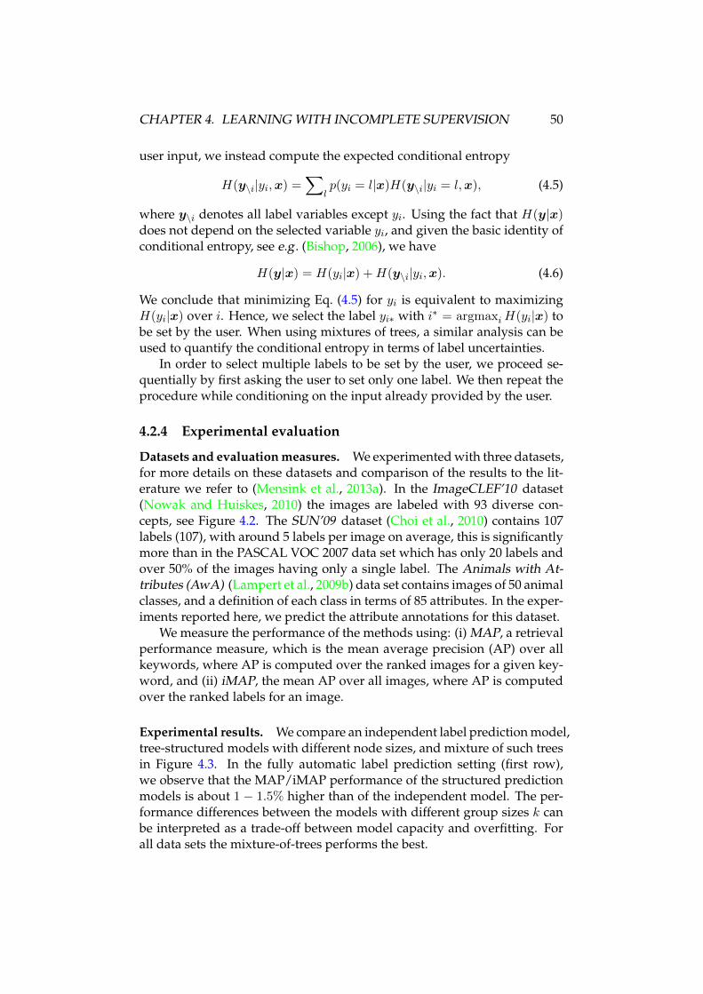
CHAPTER 4. LEARNING WITH INCOMPLETE SUPERVISION 50
user input, we instead compute the expected conditional entropy
H(y\i|yi,x) =∑
lp(yi = l|x)H(y\i|yi = l,x), (4.5)
where y\i denotes all label variables except yi. Using the fact that H(y|x)does not depend on the selected variable yi, and given the basic identity ofconditional entropy, see e.g . (Bishop, 2006), we have
H(y|x) = H(yi|x) +H(y\i|yi,x). (4.6)
We conclude that minimizing Eq. (4.5) for yi is equivalent to maximizingH(yi|x) over i. Hence, we select the label yi∗ with i∗ = argmaxiH(yi|x) tobe set by the user. When using mixtures of trees, a similar analysis can beused to quantify the conditional entropy in terms of label uncertainties.
In order to select multiple labels to be set by the user, we proceed se-quentially by first asking the user to set only one label. We then repeat theprocedure while conditioning on the input already provided by the user.
4.2.4 Experimental evaluation
Datasets and evaluation measures. We experimented with three datasets,for more details on these datasets and comparison of the results to the lit-erature we refer to (Mensink et al., 2013a). In the ImageCLEF’10 dataset(Nowak and Huiskes, 2010) the images are labeled with 93 diverse con-cepts, see Figure 4.2. The SUN’09 dataset (Choi et al., 2010) contains 107labels (107), with around 5 labels per image on average, this is significantlymore than in the PASCAL VOC 2007 data set which has only 20 labels andover 50% of the images having only a single label. The Animals with At-tributes (AwA) (Lampert et al., 2009b) data set contains images of 50 animalclasses, and a definition of each class in terms of 85 attributes. In the exper-iments reported here, we predict the attribute annotations for this dataset.
We measure the performance of the methods using: (i) MAP, a retrievalperformance measure, which is the mean average precision (AP) over allkeywords, where AP is computed over the ranked images for a given key-word, and (ii) iMAP, the mean AP over all images, where AP is computedover the ranked labels for an image.
Experimental results. We compare an independent label prediction model,tree-structured models with different node sizes, and mixture of such treesin Figure 4.3. In the fully automatic label prediction setting (first row),we observe that the MAP/iMAP performance of the structured predictionmodels is about 1 − 1.5% higher than of the independent model. The per-formance differences between the models with different group sizes k canbe interpreted as a trade-off between model capacity and overfitting. Forall data sets the mixture-of-trees performs the best.
CHAPTER 4. LEARNING WITH INCOMPLETE SUPERVISION 51
ImageCLEF’10 SUN09 AwA ImageCLEF’10 SUN09 AwAA
utom
atic
MA
P
I k1 k2 k3 k4 M40
41
42
43
44
45
I k1 k2 k3 k4 M25
30
35
I k1 k2 k3 k4 M55
60
65
iMA
P
I k1 k2 k3 k4 M75
76
77
78
79
80
I k1 k2 k3 k4 M70
71
72
73
74
75
I k1 k2 k3 k4 M70
71
72
73
74
75
nrQ
=5
MA
P
I k1 k2 k3 k4 M50
52
54
56
58
60
I k1 k2 k3 k4 M40
42
44
46
48
50
I k1 k2 k3 k4 M65
70
75
iMA
P
I k1 k2 k3 k4 M80
82
84
86
88
90
I k1 k2 k3 k4 M80
81
82
83
84
85
I k1 k2 k3 k4 M75
80
85
nrQ
=10
MA
P
I k1 k2 k3 k4 M55
60
65
70
I k1 k2 k3 k4 M45
50
55
60
I k1 k2 k3 k4 M70
75
80
85
iMA
P
I k1 k2 k3 k4 M85
90
95
I k1 k2 k3 k4 M85
86
87
88
89
90
I k1 k2 k3 k4 M80
82
84
86
88
90
Figure 4.3 – Performance for fully automated prediction (first row), andan interactive setting with 5 and 10 questions (second and third row). Foreach setting and dataset, we compare results of the independent model (I,blue), the trees with group sizes k from 1 to 4 (k1–k4, light-red), and themixture-of-trees (M, dark-red).
In the interactive image annotation scenario the system iteratively se-lects labels to be set by the user (set to the ground value in our experiments).For the independent model, the entropy-based selection procedure is alsoused, which results in setting the most uncertain labels. The annotation re-sults obtained after setting 5 respectively 10 labels are shown in the secondand third rows of Figure 4.3. Note the different vertical scales across the dif-ferent rows. As expected, in this setting the structured models benefit morefrom the user input, since they propagate the information provided by theuser to update the predictions on the remaining labels, and also avoids ask-ing input for multiple highly correlated labels. The mixture-of-trees againperforms optimal, or close to optimal, in all cases.
To assess the proposed label elicitation method we compare its perfor-mances to using a random strategy, we do so using the independent modeland the mixture-of-trees model For the random strategy we report the av-erage performance over ten experiments. The results in Figure 4.4 showthat with either elicitation mechanism, the structured model outperformsthe independent model. Furthermore, for both models the entropy-basedlabel elicitation mechanism is more effective than random selection.
4.2.5 Summary
In this section we presented tree-structured models to capture dependen-cies among image labels. We explored (i) different strategies to learn theunary potentials (pre-trained SVM classifiers and joint learning with the

CHAPTER 4. LEARNING WITH INCOMPLETE SUPERVISION 52
0 20 40 60 800.4
0.5
0.6
0.7
0.8
0.9
1
Nr Questions
MA
P
Indep − RandIndep − EntMixt − RandMixt − Ent
0 20 40 60 800.75
0.8
0.85
0.9
0.95
1
Nr Questions
iMA
P
Figure 4.4 – Comparison of the random and entropy-based label selectionfor the independent and the structured mixture-of-trees model using theImageCLEF’10 dataset.
pairwise potentials), (ii) various graphical structures (trees, trees over la-bel groups, and mixtures of trees), and (iii) methods to obtain these struc-tures (using mutual information and based on maximum likelihood). Wefind that best performance is obtained using a mixture-of-trees with differ-ent label group sizes, where the unary potentials are given by pre-trainedSVM classifiers. During training, the SVM scores are obtained in a cross-validation manner, to ensure that the quality of the SVM scores is repre-sentative of that of test images. The proposed models offer a moderate im-provement over independent baseline models in a fully automatic setting.Their main strength lies in improved predictions in an interactive imagelabeling setting.
4.3 Weakly supervised learning for object localization
For object detection, weakly supervised learning from image-wide labelsthat indicate the presence of instances of a category in images has recentlybeen intensively studied as a way to remove the need for bounding box an-notations, see e.g . (Bagon et al., 2010; Chum and Zisserman, 2007; Crandalland Huttenlocher, 2006; Deselaers et al., 2012; Pandey and Lazebnik, 2011;Prest et al., 2012; Russakovsky et al., 2012; Shi et al., 2013; Siva et al., 2012;Siva and Xiang, 2011; Song et al., 2014a,b; Bilen et al., 2014; Wang et al.,2014a). In this section, we present a method based on multiple instancelearning that interleaves training of the detector with re-localization of ob-ject instances on the positive training images. Following recent state-of-the-art work in fully supervised detection (Cinbis et al., 2013; Girshick et al.,2014; van de Sande et al., 2014), we represent tentative detection windowsusing high-dimensional Fisher vectors (140K dims.) (Sanchez et al., 2013)and convolutional neural network features (140K dims.) (Krizhevsky et al.,2012). When used in an MIL framework, the high-dimensionality of the

CHAPTER 4. LEARNING WITH INCOMPLETE SUPERVISION 53
window features makes MIL quickly convergence to poor local optima af-ter initialization. Our main contribution is a multi-fold training procedurefor MIL, which avoids this rapid convergence to poor local optima. In ad-dition, we propose a window refinement method that improves the weaklysupervised localization accuracy by incorporating a category-independentobjectness measure.
Part of this material was presented at CVPR’14 (Cinbis et al., 2014), anextended version of the paper will appear in PAMI (Cinbis et al., 2016b).The latter is available at https://hal.inria.fr/hal-01123482/file/paper_final.pdf.
4.3.1 Multi-fold training for weakly supervised localization
The majority of related work treats WSL for object detection as a multipleinstance learning (MIL) (Dietterich et al., 1997) problem. Each image is con-sidered as a “bag” of examples given by tentative object windows. Positiveimages are assumed to contain at least one positive object instance window,while negative images only contain negative windows. The object detectoris then obtained by alternating detector training, and using the detector toselect the most likely object instances in positive images.
In many MIL problems, e.g . such as those for weakly supervised facerecognition (Berg et al., 2004; Everingham et al., 2009), the number of ex-amples per bag is limited to a few dozen at most. In contrast, there is a vastnumber of examples per bag in the case of object detector training sincethe number of possible object bounding boxes is quadratic in the num-ber of image pixels. Object detection proposal methods, e.g . (Alexe et al.,2010; Gu et al., 2012; Uijlings et al., 2013; Zitnick and Dollar, 2014), can beused to make MIL approaches to WSL for object localization manageable,and make it possible to use powerful and computationally expensive ob-ject models. In our work we use the selective search method of Uijlings etal . (Uijlings et al., 2013), to generate a limited set of around 1,500 candidatewindows per image. Jointly selecting the objects across the retained win-dows across thousands of images, however, is still a challenging problemsince the number of choices is exponential in the number of images.
Note that in the MIL approach described above, the detector used forre-localization in positive images is trained using positive samples that areextracted from the very same images. Therefore, there is a bias towardsre-localizing on the same windows; in particular when high capacity clas-sifiers are used which are likely to separate the detector’s training data. Forexample, when a nearest neighbor classifier is used the re-localization willbe degenerate and not move away from its initialization, since the samewindow will be found as its nearest neighbor. The same phenomenon oc-curs when using powerful and high-dimensional image representations totrain linear classifiers. We illustrate this in the left panel of Figure 4.5, which

CHAPTER 4. LEARNING WITH INCOMPLETE SUPERVISION 54
0 0.2 0.4 0.6 0.8 10
0.2
0.4
0.6
0.8
1
Normalized Score
Fre
quen
cy
Below 50% overlapAbove 50% overlapTraining windows
−1 −0.5 0 0.5 10
0.2
0.4
0.6
0.8
High dimensional FV
Den
sity
Inner Product
Figure 4.5 – Left: distribution of the window scores in positive training im-ages during MIL training. Red: windows used for training. Green: otherwindows that overlap with them by more than 50%. Blue: windows thatoverlap less than 50%. Each curve is obtained by averaging all per-classscore distributions. The surrounding regions show the standard deviation.Right: distribution of inner products between Fisher vectors of pairs ofwindows, where each pair is sampled from within a single image.
shows the distribution of the window scores in a typical MIL iteration onVOC 2007 using Fisher vectors. We observe that the windows used in SVMtraining score significantly higher than the other ones, including those witha significant spatial overlap with the most recent training windows. As aresult, MIL typically results in degenerate re-localization.
This problem is related to the dimensionality of the window descrip-tors. We illustrate this in the right panel of Figure 4.5, where we showthe distribution of inner products between the descriptors of window pairswithin the same image. Almost all window descriptors are near orthogo-nal for the 140K dimensional FVs. Recall that the weight vector of a linearSVM classifier can be written as a linear combination of training samples,w =
∑i αixi, and the SVM score of a test sample is given by a linear com-
bination of inner products with training vectors. Therefore, the trainingwindows are likely to score significantly higher than the other windows inpositive images in the high-dimensional case, resulting in degenerate re-localization behavior.
Note that increasing regularization weight in SVM training does notremedy this problem. The `2 regularization term with weight λ restricts thelinear combination weights such that |αi| ≤ 1/λ. Therefore, although wecan reduce the influence of individual training samples via regularization,the resulting classifier remains biased towards the training windows sincethe classifier is a linear combination of the window descriptors.
To address this issue—without sacrificing the descriptor dimensional-

CHAPTER 4. LEARNING WITH INCOMPLETE SUPERVISION 55
ity, which would limit its descriptive power—we propose to train the de-tector using a multi-fold procedure, reminiscent of cross-validation, withinthe MIL iterations. We divide the positive training images into K disjointfolds, and re-localize the images in each fold using a detector trained us-ing windows from positive images in the other folds. In this manner there-localization detectors never use training windows from the images towhich they are applied. Once re-localization is performed in all positivetraining images, we train another detector using all selected windows. Thisdetector is used for hard-negative mining on negative training images, andreturned as the final detector.
The number of folds used in our multi-fold MIL training procedureshould be set to strike a trade-off between two competing factors. On theone hand, using more folds increases the number of training samples perfold, and is therefore likely to improve re-localization performance. On theother hand, using more folds increases the computational cost.
4.3.2 Window refinement
An inherent difficulty for weakly supervised object localization is that WSLlabels only permit to determine the most repeatable and discriminative pat-terns for each class. Therefore, even though the windows found by WSL arelikely to overlap with target object instances, they might not align with thefull object outline. We propose a window refinement method to update thelocalizations obtained by multi-fold training. The final detector is trainedbased on these refinements.
To explicitly take into account object boundaries, we use the edge-drivenobjectness measure of Zitnick and Dollar (Zitnick and Dollar, 2014). Themain idea of this approach is to score a given window based on the numberof contours that are fully contained inside the window, with an increasedweight on near-boundary edge pixels. Thus, windows that tightly encloselong contours are scored highly, whereas those with predominantly strad-dling contours are penalized. Additionally, in order to reduce the effect ofslight misalignments, the coordinates of a given window are updated usinga greedy local search procedure that aims to increase the objectness score.
In (Zitnick and Dollar, 2014), the objectness measure is used for gen-erating object proposals. We instead use the edge-driven objectness mea-sure to improve WSL outputs. For this purpose, we combine the objectnessmeasure with the detection scores given by multi-fold MIL. More specifi-cally, we first utilize the local search procedure in order to update and scorethe refined candidate detection windows based on the objectness measure,without updating the detection scores. To make the detection and object-ness scores comparable, we scale both scores to the range [0, 1] for all win-dows in the positive training images. We then average both scores, andselect the top detection in each image with respect to this combined score.

CHAPTER 4. LEARNING WITH INCOMPLETE SUPERVISION 56
Figure 4.6 – Illustration of window refinement. Dashed pink boxes showthe localization before refinement, and the solid yellow boxes show theresult after refinement. The right-most image in each pair shows the edgemap used to compute the objectness measure.
In order to avoid selecting the windows irrelevant for the target class, butwith a high objectness score, we restrict the search space to the top-N win-dows per image in terms of the detection score. While we use N = 10in all our experiments, we have empirically observed that the refinementmethod significantly improves the localization results for N ranging from1 to 50. The improvement is comparable for N ≥ 5.
In Figure 4.6, we show example images for the classes horse and dogtogether with the corresponding edge maps. In these images, the dashed(pink) boxes show the output of multi-fold MIL training and the solid (yel-low) boxes show the outputs of the window refinement procedure. Eventhough the initial windows are located on the object instances, they areevaluated as incorrect due to the low overlap ratios with the ground-truthones. The edge maps show that many contours, i.e . most object contours,straddle the initial window boundaries. In contrast, the refined windowshave higher percentages of fully contained contours, i.e . the contours rele-vant for the objects.
4.3.3 Experimental evaluation
For our experiments we used the PASCAL VOC 2007 dataset (Everinghamet al., 2010). We use linear SVM classifiers, and set the weight of the regular-ization term and the class weighting to fixed values based on preliminaryexperiments. We perform two hard-negative mining steps (Felzenszwalbet al., 2010) after each re-localization phase.
Following (Deselaers et al., 2012), we assess performance using twomeasures. First, we evaluate the fraction of positive training images inwhich we obtain correct localization (CorLoc). Second, we measure thefinal object detection performance on the test images using the standardprotocol (Everingham et al., 2010): average precision (AP) per class, sum-marized by the mean AP (mAP) across all 20 classes. For both measures, awindow is considered correct if it has an intersection-over-union ratio of atleast 50% with a ground-truth object.

CHAPTER 4. LEARNING WITH INCOMPLETE SUPERVISION 57
Corloc mAPFV CNN FV+CNN FV CNN FV+CNN
Standard MIL 29.7 41.2 34.4 15.5 24.3 22.0Multi-fold MIL 38.8 45.0 47.3 22.4 25.9 27.4
+Refinement 46.1 54.2 52.0 23.3 28.6 30.2
Table 4.1 – Comparison of standard and multi-fold MIL training, and theeffect of window refinement. Performance both in CorLoc on the positivetraining images (left), and in mAP on the test images. Results are averagedover the 20 object categories in PASCAL VOC’07.
In Table 4.1 we give a brief summary of the results of the extensive setof experiments we conducted, more details can be found in (Cinbis et al.,2016b). We report the CorLoc and mAP values across all classes for boththe FV and CNN features, as well as their combination. In all settings, andaccording to both measures, both the multi-fold training procedure and thewindow refinement bring significant improvements to the performance ofthe detectors. The improvement due to multi-fold training is more pro-nounced when using the 140K dimensional FV representation. The CNNdescriptors are only 4K dimensional, and are therefore to a lesser degreeaffected by the near-orthogonality of window descriptors observed in Fig-ure 4.5.
Our results are comparable to the current state of the art. For exampleBilen and Vedaldi (Bilen and Vedaldi, 2016) report 30.6% mAP and 51%CorLoc using a two-stream CNN approach based on the same detectionproposal windows, which finetune the CNN weights.
4.3.4 Summary
We presented a multi-fold multiple instance learning approach for weaklysupervised object detection. It improves localization performance by sep-arating the image sets for re-localization and model training. We also pre-sented a window refinement method, which improves the localization ac-curacy by using an edge-driven objectness prior.
We have evaluated our approach and compared it to state-of-the-artmethods using the VOC 2007 dataset. Our results show that multi-foldMIL effectively handles high-dimensional descriptors, which allows us toobtain results that are competitive with the state of the art by combiningFV and CNN features.
A detailed analysis of our results shows that, in terms of test set de-tection performance, multi-fold MIL attains 68% of the MIL performanceupper-bound, which we measure by selecting one correct training examplefrom each positive image, for the combined FV and CNN features.
CHAPTER 4. LEARNING WITH INCOMPLETE SUPERVISION 58
4.4 Summary and outlook
In this chapter we presented an overview of our contributions related tolearning visual models from incomplete supervision, and highlighted twoof them. In the first we model semantic image label dependencies, whichallows us to leverage user provided information on part of the labels tobetter predict the remaining unknown ones. The model also allows to inferwhich labels are most informative when given by the user. Experimentalresult demonstrate the effectiveness of this model for interactive image la-beling. The second contribution is a multi-fold multiple-instance learningframework, which we apply to learning object category localization modelsfrom weakly supervised data. In this case the training data only indicatesif an object category is present in an image, but now where.
While fully supervised methods to learn visual recognition models de-liver the best performance in general, they come with the important draw-back of requiring large and carefully annotated datasets. Collecting suchdatasets in practice is often time consuming, expensive, and not-trivial tosetup. As an example consider collecting annotations for semantic videosegmentation, where full supervision requires labeling each pixel in eachframe with a corresponding category label. Learning from incomplete formsof supervision is an important topic of research in computer vision andmachine learning in general, which can alleviate the costs of collectingsupervised datasets. The advent of deep visual recognition models onlyunderlines the importance of this issue, due to their large number of pa-rameters. Weakly supervised learning is most often expressed as learn-ing parameters of latent variable models, where the latent variables corre-spond to the missing supervision. Learning is then done with algorithmssuch as Expectation-Maximization (Dempster et al., 1977), or simple vari-ants such as multiple instance learning (Dietterich et al., 1997). Latent vari-able models beyond tree-structured factor graphs require approximate in-ference techniques, see e.g . (Verbeek and Triggs, 2008), and the effect of theprecise inference method on the learned model are relatively poorly under-stood (Kulesza and Pereira, 2008). Recent work (Zheng et al., 2015; Schwingand Urtasun, 2015) interprets variational mean-field inference as a recur-rent neural network through which error signals can be back-propagated.This ensures that the model parameters are learned directly to predict wellwhen combined with the chosen inference method. Generalization of thisprinciple is an interesting line for future work that could address the fol-lowing questions. How to re-formulate more powerful approximate infer-ence methods, such as generalized loopy belief propagation (Yedidia et al.,2002), or expectation propagation (Minka, 2001), as recurrent networks?How to incorporate higher-order potential functions in such approaches,beyond very specific restrictive classes (Arnab et al., 2015).

Chapter 5
Conclusion and perspectives
In this concluding chapter we summarize the contributions described in theprevious chapters in Section 5.1, and identify several long-term researchdirections in Section 5.2.
5.1 Summary of contributions
Below we briefly review the previous chapters, and discuss related direc-tions for future research.
Fisher vector representations. In Chapter 2 we discussed our contribu-tions around the Fisher vector (FV) image representation in the context ofrelated work. These include the derivation of the Fisher information ma-trix w.r.t. the mixing weights in (Sanchez et al., 2013), modeling the lay-out of local descriptors with a FV that represents the distribution of spatialcoordinates of each visual word (Krapac et al., 2011), and using approxi-mate segmentation masks to weight the contribution of local descriptors inthe FV for object localization (Cinbis et al., 2013). In (Cinbis et al., 2012,2016a) we presented models for local image descriptors that avoid the i.i.d.assumption that underlies the BoV and FV representations. These modelsnaturally lead to discounting effects and consequent performance improve-ments, which are comparable to those obtained using power normalization.Using our models we can interpret power-normalization as an approximatemanner to account for mutual dependencies of local descriptors. In (Oneataet al., 2014b) we presented approximations to the power and `2 normaliza-tions of the FV. Using these approximations linear score functions of thenormalized FV can be computed efficiently using integral images, since theinteraction of the weight vector with local descriptors is additive per visualword. Experimental results show that a speed-up of more than an order ofmagnitude is obtained, while having only a limited impact on localizationperformance.
59

CHAPTER 5. CONCLUSION AND PERSPECTIVES 60
The Fisher kernel framework has shown to be one of the most effec-tive methods to encode the distribution of local features in images andvideos (Chatfield et al., 2011; Oneata et al., 2013). Recently there has been amajor focus in computer vision on convolutional neural network (CNN)approaches following the success of such models at the 2012 ImageNetchallenge (Krizhevsky et al., 2012). Recent work also explored hybrid ap-proaches that combine aspects of local feature pooling and (convolutional)neural networks (Cimpoi et al., 2015; Perronnin and Larlus, 2015; Arand-jelovic et al., 2015). In particular, using a FV to aggregate local convolu-tional filters learned with a CNN, was shown in (Cimpoi et al., 2015) to im-prove over using higher-level CNN represenatations for transfer learningproblems. We believe that developing Fisher kernels for generative modelsthat capture more structural aspects is an interesting direction of future re-search. Recent examples in this direction include (Sun and Nevatia, 2013;Nagel et al., 2015), which uses a FV representation for video event recog-nition based on a hidden Markov models and Student-t distributions, and(Sanchez and Redolfi, 2015) which derives general exponential family FVrepresentations e.g . to model positive definite matrices, or binary data.
Metric learning approaches. We presented our contributions related tometric learning in Chapter 3. In (Guillaumin et al., 2009b) we presentedLDML, a logistic discriminant Mahanalobis metric learning approach, anda non-parametric marginalized nearest neighbor approach. We extendedLDML in (Guillaumin et al., 2010b) to learn low-rank Mahalanobis metrics,and to use it in combination with kernel functions. In (Guillaumin et al.,2009a) we presented a nearest neighbor image annotation model, whereinstead of using equal weights for a fixed number of neighbors, we use aweighted combination of predictions made by neighboring images. We setthe weights either based on the neighbor rank, or based on a learned com-bination of several distance metrics between images. In (Mensink et al.,2013b) we presented a Mahalanobis metric learning approach for the near-est class mean (NCM) classifier. Unlike the nearest neighbor (NN) clas-sifier, this is an efficient linear classifier. We also considered a non-linearextension where each class is represented with several centroids that canrepresent sub-classes. In our experiments we found NCM to outperformNN classification, while at the same time also being computationally moreefficient.
While most work on metric learning considers a supervised setting, itis also possible to learn metrics from unsupervised data. For example,in (Cinbis et al., 2011) we used face tracks in videos in combination withsimple temporal constraints to derive training examples for LDML metriclearning. Similarly, co-occurrence statistic have been used to learn vecto-rial word representations from unsupervised text corpora. For example,

CHAPTER 5. CONCLUSION AND PERSPECTIVES 61
the skip-gram model (Mikolov et al., 2013a,b) learns a word embedding sothat words that frequently occur nearby in text are also co-located in thelearned embedding. It is an interesting direction of future research to ex-plore similar approaches to learn metrics for visual representations. Forexample, we can learn a metric and corresponding data represenation sothat video frames that appear nearby in the same video tend to be closeaccording to the learned metric, and that frames of different videos tendto be far apart. We expect to be able to learn high-level semantic represen-tations in this manner, since even if the objects depicted in nearby videoframes might be completely disjoint, we still expect the visual content to besemantically related if they are sampled relatively nearby in time from thesame video. Recent examples of work along these lines include (Doerschet al., 2015; Isola et al., 2016; Wang and Gupta, 2015; Dosovitskiy et al., 2014;Zou et al., 2012). The motivation underlying these works is that natural vi-sual data exhibits many structural regularities, which may be exploited tolearn representations or to regularize supervised learning. This is a partic-ularly relevant line of work in the current era of powerful (convolutional)neural networks, which have extremely large numbers of parameters, andwhich are non-trivial to learn and regularize.
Learning with incomplete supervision. In Chapter 4 we presented ourcontributions related to learning from incomplete supervision. These in-clude image re-ranking models that generalize to new queries (Krapac et al.,2010), semi-supervised image classification models that leverage user pro-vided keywords for training (Guillaumin et al., 2010a), approaches to as-sociate names and faces in captioned news images and in videos (Guil-laumin et al., 2008; Mensink and Verbeek, 2008; Guillaumin et al., 2010b;Cinbis et al., 2011; Guillaumin et al., 2012), and semantic image segmenta-tion models that can be learned from incomplete supervision (Verbeek andTriggs, 2007, 2008). We developed tree-structured models over labels forinteractive image annotation (Mensink et al., 2011, 2013a) exploiting key-word dependencies to gather more informative user input and improvepredictions. Finally, we developed a multi-fold multiple instance learn-ing approach for weakly supervised object localization (Cinbis et al., 2014,2016b), which avoids poor local optima during learning and consequentlyimproves the localization performance.
In ongoing research we work on learning semantic video segmentationmodels from weak supervision, including separately segmenting individ-ual category instances. Recent advances in object localization and semanticsegmentation have revealed a number of effective techniques, which areyet to be combined in a larger overall model. These include pooling oper-ators over variable-sized areas (Ren et al., 2015; He et al., 2014), fully con-nected CRFs (Krahenbuhl and Koltun, 2011) and convolutional and decon-

CHAPTER 5. CONCLUSION AND PERSPECTIVES 62
volutional computation of unary potentials (Long et al., 2015; Ronnebergeret al., 2015; Noh et al., 2015), non-trivial data-dependent and trainable pair-wise potentials (Lin et al., 2016), recurrent networks for approximate vari-ational inference intregrated in the training process (Schwing and Urtasun,2015; Zheng et al., 2015), and the use of (linearly) constrained variationalinference for weakly supervised learning (Pathak et al., 2015). Object lo-calization models, possibly learned from image-wide labels as in (Cinbiset al., 2014), can be used to define strong prior distributions for semanticsegmentation, e.g . as in (Ladicky et al., 2010). Moreover, the strong tempo-ral correlation patterns in the label maps in semantic video segmentationsuggests the use of recurrent models to exploit this structure.
5.2 Long-term research directions
We now conclude with several more general long-term research directions.
Learning higher-order structured prediction models. Many problems incomputer vision involve joint prediction of many response variables. Ex-amples include, but are not limited to, semantic segmentation, optical flowestimation, depth estimation, image de-noising, super resolution, coloriza-tion, pose estimation, etc . These structured prediction tasks are typicallysolved using (conditional) Markov random fields, which includes unaryterms for each label variable, and pairwise terms to ensure structural regu-larity of the output predictions.
Deep networks have been used for such tasks (Long et al., 2015) to de-fine unary and pairwise terms (Lin et al., 2016). Deep networks allow com-plex functions to be learned between a label variable and a large part of allinput variables, if not all. Moreover, recently (Zheng et al., 2015; Schwingand Urtasun, 2015) it has been shown that variational mean-field inferencein Markov random fields can be expressed as a special recurrent neural net-works in the case of fully connected pair-wise energy functions. This allowsthe training of the unary and pairwise potentials to be done in a way thatis coherent with the MRF structure and the approximate inference method.
Higher-order potentials, that model interactions of more than two labelvariables at a time, have been proven effective in the past for structuredprediction tasks, see e.g . (Kohli et al., 2009). Efficient inference, however,is only possible for a very specific classes of higher-order potentials, seee.g . (Vineet et al., 2014; Ramalingam et al., 2008). An exiting direction forfuture work is to consider how larger classes of trainable higher-order po-tentials can be used by generalizing the techniques developed in (Zhenget al., 2015; Schwing and Urtasun, 2015) for pairwise structured models.The work of Pinheiro and Collobert on recurrent convolutional networks(Pinheiro and Collobert, 2014) is also highly relevant in this area. An al-
CHAPTER 5. CONCLUSION AND PERSPECTIVES 63
ternative route to enforce higher-order regularity in the predictions mightbe to used adversarial networks (Goodfellow et al., 2014) that are trainedin combination with the primary prediction model. The adversarial net-work is trained to discriminate ground-truth samples and samples fromthe primary model. The primary model is trained such that the adversarialnetwork can not discriminate samples from the primary model from sam-ples of the ground-truth. The adversarial network may be used to enforcehigher-order consistency, even if higher-order potentials are not used in theprimary model. The development of models that exhibit high-order regu-larities which are trainable in a data-driven manner are likely to have ansignificant impact across a wide variety of multivariate and dense predic-tion vision problems.
Learning from minimal supervision. An important bottleneck limitingperformance of visual recognition systems in practical applications is thereliance on supervised training dataset. Generally, supervision is expensiveand time consuming to collect. There are at least three different paths tomake up for a lack of supervised training data.
The first is to learn models that to go beyond recognizing (i.e . classify-ing, localizing, segmenting, etc .) a manually specified finite list of (object)categories. Approaches in this direction include semantic word-image em-bedding models such as DeViSE (Frome et al., 2013), and image-captionencoder-decoder models (Kiros et al., 2015). Such models can in princi-ple be learned from large non-curated datasets which contain images with(loosely) associated textual descriptions (general web images, wikipedia,user generated content, etc .), see e.g . (Chen et al., 2013b). This approach,combined with word-embedding techniques (Mikolov et al., 2013b) and“on-the-fly” model learning from web image-search engines (Chatfield et al.,2015), allows to learn bi-directional image-text mappings that can be usedfor example for free-text visual search in large image and video datasets,without requiring any manually curated supervised training datasets.
Second, for certain critical visual recognition tasks that require high-level of accuracy (e.g . advanced driver assistance systems, or defense re-lated applications), manually collected supervised training datasets will berequired to ensure sufficient accuracy. In such cases the question is howwe can make the most out of the (limited) available training data. An ideathat has proven extremely effective is to use auxiliary tasks to pre-train orinitialize the recognition model, see e.g . (Girshick et al., 2014). Most oftenpre-training is based on large supervised training datasets; with ImageNet(Deng et al., 2009) being by far the most used dataset for this purpose.Large unsupervised datasets may also be used for this purpose, by definingauxiliary tasks based on spatial or temporal structure (Doersch et al., 2015;Wang and Gupta, 2015; Isola et al., 2016). Most work takes a rather ad-hoc
CHAPTER 5. CONCLUSION AND PERSPECTIVES 64
approach of taking a pre-trained model, and adapting it to the task at hand.In a more principled manner, we can learn by jointly minimizing the loss ofthe (new) target task and a loss for the (earlier) auxiliary task(s). Pushingthis idea further, a “life-long” learning scheme is interesting in which wetrain a single large model for an increasing number of tasks. Treating the“old” tasks a pre-training or regularization for the new tasks.
Finally, a third approach is to rely on contextual cues. These can ei-ther in the form of spatial inter-object context, see e.g . (Rabinovich et al.,2007; Choi et al., 2010), or between objects and physical scene propertiessuch as scene geometry estimates, see e.g . (A. Geiger and Urtasun, 2011;Hoiem et al., 2008). Another form of context is to use complex data adap-tive non-parametric priors on the parameters of discriminative recognitionmodels, see e.g . (Salakhutdinov et al., 2012). Such priors can infer hierar-chical groupings of object categories, so that training data is shared to someextent between related classes.
These three paragraphs may be summarized as follows. (i) For someproblems abundantly available and loosely annotated training data maybe enough to learn satisfying models, e.g . for text-based image search. (ii)In cases where this is not sufficient, auxiliary tasks may be used for pre-training, or multi-task learning can be used as a regularization principle tomake up for lack of supervised training data. (iii) Contextual informationof various forms can provide stronger structuring information. Future re-search on combining these different approaches may lead to important ad-vances in learning visual recognition models from very little training data,which may have significant impact for practical applications.
Architecture learning and adaptation. Current state of the art high-levelsemantic scene understanding models are dominated by (convolutional)neural network approaches. These models are very powerful due to theirstrong capacity to model complex data distributions, which results froma hierarchical structure with millions configurable parameters that can beautomatically tuned based on (supervised) training data (Montufar et al.,2014). Beyond the challenges to efficiently estimate such models from lim-ited training data, an even bigger challenge is posed by the model selectionproblem. That is: how to determine the best, or a “good”, architecturefor such models? This includes: the number and ordering of pooling andconvolutional layers, filter sizes, number of channels, type of pooling op-erations, type of non-linearities, etc . This problem is extremely hard, sincethe space of possible network architectures is discrete and combinatoriallylarge. Optimizing over this space is an important challenge for future re-search. Work in this direction includes using sparsity inducing regularizersto sparsify the connectivity pattern (Kulkarni et al., 2015), and using sparsehierarchical priors over the network structure in a Bayesian learning frame-

CHAPTER 5. CONCLUSION AND PERSPECTIVES 65
work (Adams et al., 2010).In the context of extremely large datasets, such as those used for learn-
ing from weakly supervised sources discussed above, model selection mightnot be the right problem to consider. Instead of searching for the single ul-timate model architecture, it will be important to progressively adapt themodel architecture and capacity during learning. That is: having seen littledata it might be useful to limit the degrees of freedom of the model. As thelearning algorithm sees more data the limited capacity will saturate, andmore capacity should be allocated. This suggests that studying a dynamicvariant of the model selection problem is perhaps more important.
The model selection problem is highly challenging, but progress is likelyto have big impact across many computer vision problems and beyond.

Bibliography
The zettabyte era: Trends and analysis. White Paper, 2015.http://www.cisco.com/c/en/us/solutions/collateral/service-provider/visual-networking-index-vni/VNI_Hyperconnectivity_WP.pdf.
C. Wojek A. Geiger and R. Urtasun. Joint 3d estimation of objects and scenelayout. In NIPS, 2011.
R. Adams, H. Wallach, and Z. Ghahramani. Learning the structure of deepsparse graphical models. In AISTATS, 2010.
B. Alexe, T. Deselaers, and V. Ferrari. What is an object? In CVPR, 2010.
B. Alexe, T. Deselares, and V. Ferrari. Measuring the objectness of imagewindows. PAMI, 34(11):2189–2202, 2012.
R. Arandjelovic and A. Zisserman. Three things everyone should know toimprove object retrieval. In CVPR, 2012.
R. Arandjelovic, P. Gronat, A. Torii, T. Pajdla, and J. Sivic. NetVLAD: CNNarchitecture for weakly supervised place recognition. Arxiv preprint,2015.
A. Arnab, S. Jayasumana, S. Zheng, and P. Torr. Higher order potentialsin end-to-end trainable conditional random fields. 2015. URL http://arxiv.org/abs/1511.08119.
S. Bagon, O. Brostovski, M. Galun, and M. Irani. Detecting and sketchingthe common. In CVPR, 2010.
B. Bai, J. Weston, D. Grangier, R. Collobert, K. Sadamasa, Y. Qi, O. Chapelle,and K. Weinberger. Learning to rank with (a lot of) word features. Infor-mation Retrieval, 13(3):291–314, 2010.
K. Barnard, P. Duygulu, D. Forsyth, N. de Freitas, D. Blei, and M. Jordan.Matching words and pictures. JMLR, 3:1107–1135, 2003.
66

BIBLIOGRAPHY 67
R. Bekkerman and J. Jeon. Multi-modal clustering for multimedia collec-tions. In CVPR, 2007.
A. Bellet, A. Habrard, and M. Sebban. A Survey on Metric Learning forFeature Vectors and Structured Data. ArXiv e-prints, 1306.6709, 2013.
S. Bengio, J. Weston, and D. Grangier. Label embedding trees for largemulti-class tasks. In NIPS, 2011.
T. Berg and D. Forsyth. Animals on the web. In CVPR, 2006.
T. Berg, A. Berg, J. Edwards, M. Maire, R. White, Y. Teh, E. Learned-Miller,and D. Forsyth. Names and faces in the news. In CVPR, 2004.
H. Bilen and A. Vedaldi. Weakly supervised deep detection networks. InCVPR, 2016.
H. Bilen, M. Pedersoli, and T. Tuytelaars. Weakly supervised object detec-tion with posterior regularization. In BMVC, 2014.
C. Bishop. Pattern recognition and machine learning. Spinger-Verlag, 2006.
L. Bottou. Large-scale machine learning with stochastic gradient descent.In COMPSTAT, 2010.
J. Bradley and C. Guestrin. Learning tree conditional random fields. InICML, 2010.
S. Branson, C. Wah, F. Schroff, B. Babenko, P. Welinder, P. Perona, and S. Be-longie. Visual recognition with humans in the loop. In ECCV, 2010.
T. Brox and J. Malik. Object segmentation by long term analysis of pointtrajectories. In ECCV, 2010.
G. Carneiro, A. Chan, P. Moreno, and N. Vasconcelos. Supervised learningof semantic classes for image annotation and retrieval. PAMI, 29(3):394–410, 2007.
K. Chatfield, V. Lempitsky, A. Vedaldi, and A. Zisserman. The devil is inthe details: an evaluation of recent feature encoding methods. In BMVC,2011.
K. Chatfield, R. Arandjelovic, O. Parkhi, and A. Zisserman. On-the-flylearning for visual search of large-scale image and video datasets. In-ternational Journal of Multimedia Information Retrieval, 2015.
Q. Chen, Z. Song, R. Feris, A. Datta, L. Cao, Z. Huang, and S. Yan. Efficientmaximum appearance search for large-scale object detection. In CVPR,2013a.

BIBLIOGRAPHY 68
X. Chen, A. Shrivastava, and A. Gupta. NEIL: Extracting visual knowledgefrom web data. In ICCV, 2013b.
M. Cho, S. Kwak, C. Schmid, and J. Ponce. Unsupervised object discoveryand localization in the wild. In CVPR, 2015.
M. Choi, J. Lim, A. Torralba, and A. Willsky. Exploiting hierarchical contexton a large database of object categories. In CVPR, 2010.
S. Chopra, R. Hadsell, and Y. LeCun. Learning a similarity metric discrim-inatively, with application to face verification. In CVPR, 2005.
C. Chow and C. Liu. Approximating discrete probability distributions withdependence trees. IEEE Trans. Information Theory, 14(3):462–467, 1968.
O. Chum and A. Zisserman. An exemplar model for learning object classes.In CVPR, 2007.
M. Cimpoi, S. Maji, and A. Vedaldi. Deep filter banks for texture recogni-tion and segmentation. In CVPR, 2015.
R. Cinbis, J. Verbeek, and C. Schmid. Unsupervised metric learning for faceidentification in TV video. In ICCV, 2011.
R. Cinbis, J. Verbeek, and C. Schmid. Image categorization using Fisherkernels of non-iid image models. In CVPR, 2012.
R. Cinbis, J. Verbeek, and C. Schmid. Segmentation driven object detectionwith Fisher vectors. In ICCV, 2013.
R. Cinbis, J. Verbeek, and C. Schmid. Multi-fold mil training for weaklysupervised object localization. In CVPR, 2014.
R. Cinbis, J. Verbeek, and C. Schmid. Approximate Fisher kernels of non-iidimage models for image categorization. PAMI, 2016a.
R. Cinbis, J. Verbeek, and C. Schmid. Weakly supervised object localizationwith multi-fold multiple instance learning. PAMI, 2016b. to appear.
C. Cortes and V. Vapnik. Support-vector networks. Machine Learning, 20(3):273–297, 1995.
D. Crandall and D. Huttenlocher. Weakly supervised learning of part-basedspatial models for visual object recognition. In ECCV, 2006.
G. Csurka and F. Perronnin. An efficient approach to semantic segmenta-tion. IJCV, 95(2):198–212, 2011.

BIBLIOGRAPHY 69
G. Csurka, C. Dance, L. Fan, J. Willamowski, and C. Bray. Visual categoriza-tion with bags of keypoints. In ECCV Int. Workshop on Stat. Learning inComputer Vision, 2004.
N. Dalal and B. Triggs. Histograms of oriented gradients for human de-tection. In CVPR, 2005. doi: 10.1109/CVPR.2005.177. URL http://hal.inria.fr/inria-00548512.
J. Davis, B. Kulis, P. Jain, S. Sra, and I. Dhillon. Information-theoretic metriclearning. In ICML, 2007.
A. Dempster, N. Laird, and D. Rubin. Maximum likelihood from incom-plete data via the EM algorithm. Journal of the Royal Statistical Society.Series B (Methodological), 39(1):1–38, 1977.
J. Deng, W. Dong, R. Socher, L.-J. Li, K. Li, and L. Fei-Fei. Imagenet: Alarge-scale hierarchical image database. In CVPR, 2009.
J. Deng, A. Berg, K. Li, and L. Fei-Fei. What does classifying more than10,000 image categories tell us? In ECCV, 2010.
T. Deselaers, B. Alexe, and V. Ferrari. Localizing objects while learning theirappearance. In ECCV, 2010.
T. Deselaers, B. Alexe, and V. Ferrari. Weakly supervised localization andlearning with generic knowledge. IJCV, 100(3):257–293, 2012.
T. Dietterich, R. Lathrop, and T. Lozano-Perez. Solving the multiple in-stance problem with axis-parallel rectangles. Artificial Intelligence, 89(1-2):31–71, 1997.
C. Doersch, A. Gupta, and A. Efros. Unsupervised visual representationlearning by context prediction. In ICCV, 2015.
A. Dosovitskiy, J. Springenberg, M. Riedmiller, and T. Brox. Discriminativeunsupervised feature learning with convolutional neural networks. InNIPS, 2014.
O. Duchenne, I. Laptev, J. Sivic, F. Bach, and J. Ponce. Automatic annotationof human actions in video. In ICCV, 2009.
M. Everingham, J. Sivic, and A. Zisserman. ‘Hello! My name is... Buffy’ -automatic naming of characters in TV video. In BMVC, 2006.
M. Everingham, J. Sivic, and A. Zisserman. Taking the bite out of automaticnaming of characters in TV video. Image and Vision Computing, 27(5):545–559, 2009.

BIBLIOGRAPHY 70
M. Everingham, L. van Gool, C. Williams, J. Winn, and A. Zisserman. Thepascal visual object classes (VOC) challenge. IJCV, 88(2):303–338, June2010.
P. Felzenszwalb, R. Grishick, D. McAllester, and D. Ramanan. Object de-tection with discriminatively trained part based models. PAMI, 32(9),2010.
S. Feng, R. Manmatha, and V. Lavrenko. Multiple Bernoulli relevance mod-els for image and video annotation. In CVPR, 2004.
R. Fergus, P. Perona, and A. Zisserman. A visual category filter for Googleimages. In ECCV, 2004.
R. Fergus, L. Fei-Fei, P. Perona, and A. Zisserman. Learning object cate-gories from Google’s image search. In ICCV, 2005.
B. Fernando, E. Gavves, J. Oramas, A. Ghodrati, and T. Tuytelaars. Model-ing video evolution for action recognition. In CVPR, 2015.
A. Frome, G. Corrado, J. Shlens, S. Bengio, J. Dean, M. Ranzato, andT. Mikolov. DeViSE: A deep visual-semantic embedding model. In NIPS,2013.
T. Gao and D. Koller. Discriminative learning of relaxed hierarchy for large-scale visual recognition. In ICCV, 2011.
R. Girshick, J. Donahue, T. Darrell, and J. Malik. Rich feature hierarchiesfor accurate object detection and semantic segmentation. In CVPR, 2014.
A. Globerson and S. Roweis. Metric learning by collapsing classes. In NIPS,2006.
I. Goodfellow, J. Pouget-Abadie, M. Mirza, B. Xu, D. Warde-Farley, S. Ozair,A. Courville, and Y. Bengio. Generative adversarial nets. In NIPS, 2014.
D. Grangier and S. Bengio. A discriminative kernel-based model to rankimages from text queries. PAMI, 30(8):1371–1384, 2008.
K. Gregor, I. Danihelka, A. Graves, and D. Wierstra. Draw: A recurrentneural network for image generation view publication. In icml, 2015.
C. Gu, P. Arbelaez, Y. Lin, K. Yu, and Malik. Multi-component models forobject detection. In ECCV, 2012.
M. Guillaumin, T. Mensink, J. Verbeek, and C. Schmid. Automatic facenaming with caption-based supervision. In CVPR, 2008.

BIBLIOGRAPHY 71
M. Guillaumin, T. Mensink, J. Verbeek, and C. Schmid. Tagprop: Dis-criminative metric learning in nearest neighbor models for image auto-annotation. In ICCV, 2009a.
M. Guillaumin, J. Verbeek, and C. Schmid. Is that you? Metric learningapproaches for face identification. In ICCV, 2009b.
M. Guillaumin, J. Verbeek, and C. Schmid. Multimodal semi-supervisedlearning for image classification. In CVPR, 2010a.
M. Guillaumin, J. Verbeek, and C. Schmid. Multiple instance metric learn-ing from automatically labeled bags of faces. In ECCV, 2010b.
M. Guillaumin, T. Mensink, J. Verbeek, and C. Schmid. Face recognitionfrom caption-based supervision. IJCV, 96(1):64–82, 2012.
J. Hays and A. Efros. im2gps: estimating geographic information from asingle image. In CVPR, 2008.
K. He, X. Zhang, S. Ren, and J. Sun. Spatial pyramid pooling in deep con-volutional networks for visual recognition. In ECCV, 2014.
G. Hinton, P. Dayan, B. Frey, and R. Neal. The wake-sleep algorithm forunsupervised neural networks. Science, 268:1158–1161, 1995.
D. Hoiem, A. Efros, and M. Hebert. Putting objects in perspective. IJCV,80:3–15, 2008.
P. Isola, D. Zoran, D. Krishnan, and E. Adelson. Learning visual groupsfrom co-occurrences in space and time. In ICLR, 2016.
T. Jaakkola and D. Haussler. Exploiting generative models in discrimina-tive classifiers. In NIPS, 1999.
H. Jegou, M. Douze, and C. Schmid. On the burstiness of visual elements.In CVPR, 2009.
H. Jegou, F. Perronnin, M. Douze, J. Sanchez, P. Perez, and C. Schmid. Ag-gregating local image descriptors into compact codes. PAMI, 34(9):1704–1716, 2012.
J. Jeon, V. Lavrenko, and R. Manmatha. Automatic image annotation andretrieval using cross-media relevance models. In ACM SIGIR, 2003.
Y.-G. Jiang, J. Liu, A. Roshan Zamir, G. Toderici, I. Laptev, M. Shah, andR. Sukthankar. THUMOS challenge: Action recognition with a largenumber of classes. http://crcv.ucf.edu/THUMOS14, 2014.
M. Jordan, editor. Learning in Graphical Models. Kluwer, 1998.
BIBLIOGRAPHY 72
M. Jordan, Z. Ghahramani, T. Jaakola, and L. Saul. An introduction to vari-ational methods for graphical models. Machine Learning, 37(2):183–233,1999.
A. Joulin, F. Bach, and J. Ponce. Discriminative clustering for image co-segmentation. In CVPR, 2010.
A. Joulin, K. Tang, and L. Fei-Fei. Efficient image and video co-localizationwith Frank-Wolfe algorithm. In ECCV, 2014.
F. Khan, R. Anwer, J. van de Weijer, A. Bagdanov, M. Vanrell, and A. Lopez.Color attributes for object detection. In CVPR, 2012.
R. Kiros, R. Salakhutdinov, and R. Zemel. Unifying visual-semantic embed-dings with multimodal neural language models. TACL, 2015. to appear.
Takumi Kobayashi. Dirichlet-based histogram feature transform for imageclassification. In CVPR, 2014.
P. Kohli, L. Ladicky, and P. Torr. Robust higher order potentials for enforc-ing label consistency. IJCV, 82(3):302–324, 2009.
M. Kostinger, M. Hirzer, P. Wohlhart, P. Roth, and H. Bischof. Large scalemetric learning from equivalence constraints. In CVPR, 2012.
P. Krahenbuhl and V. Koltun. Efficient inference in fully connected crfs withgaussian edge potentials. In NIPS, 2011.
J. Krapac, M. Allan, J. Verbeek, and F. Jurie. Improving web-image searchresults using query-relative classifiers. In CVPR, 2010.
J. Krapac, J. Verbeek, and F. Jurie. Modeling spatial layout with Fishervectors for image categorization. In ICCV, 2011.
A. Krizhevsky, I. Sutskever, and G. Hinton. Imagenet clas-sification with deep convolutional neural networks. InNIPS, 2012. URL http://papers.nips.cc/paper/4824-imagenet-classification-with-deep-convolutional-neural-networks.pdf.
A. Kulesza and F. Pereira. Structured learning with approximate inference.In NIPS, 2008.
B. Kulis. Metric learning: A survey. Foundations and Trends in MachineLearning, 5(4):287–364, 2012.
P. Kulkarni, J. Zepeda, F. Jurie, P. Perez, and L. Chevallier. Learning thestructure of deep architectures using l1 regularization. In BMVC, 2015.

BIBLIOGRAPHY 73
L. Ladicky, P. Sturgess, K. Alahari, C. Russell, and P. Torr. What, where &how many? combining object detectors and crfs. In ECCV, 2010.
C. Lampert, M. Blaschko, and T. Hofmann. Efficient subwindow search:a branch and bound framework for object localization. PAMI, 31(12):2129–2142, 2009a.
C. Lampert, H. Nickisch, and S. Harmeling. Learning to detect unseenobject classes by between-class attribute transfer. In CVPR, 2009b.
I. Laptev and P. Perez. Retrieving actions in movies. In ICCV, 2007.
V. Lavrenko, R. Manmatha, and J. Jeon. A model for learning the semanticsof pictures. In NIPS, 2003.
S. Lazebnik, C. Schmid, and J. Ponce. Beyond bags of features: spatialpyramid matching for recognizing natural scene categories. In CVPR,2006.
Y. LeCun, B. Boser, J. Denker, D. Henderson, R. Howard, W. Hubbard, andL. Jackel. Handwritten digit recognition with a back-propagation net-work. In NIPS, 1989.
T. Leung and J. Malik. Representing and recognizing the visual appearanceof materials using three-dimensional textons. IJCV, 43(1):29–44, 2001.
J. Li and J. Wang. Real-time computerized annotation of pictures. PAMI, 30(6):985–1002, 2008.
L.-J. Li, G. Wang, and L. Fei-Fei. OPTIMOL: Automatic object picture col-lection via incremental model learning. In CVPR, 2007.
Z. Li, E. Gavves, K. van de Sande, C. Snoek, and A. Smeulders. Codemaps,segment classify and search objects locally. In ICCV, 2013.
G. Lin, C. Shen, A. van den Hengel, and I. Reid. Efficient piecewise trainingof deep structured models for semantic segmentation. In CVPR, 2016.
Y. Lin, F. Lv, S. Zhu, M. Yang, T. Cour, K. Yu, L. Cao, and T. Huang. Large-scale image classification: Fast feature extraction and SVM training. InCVPR, 2011.
J. Liu, M. Li, Q. Liu, H. Lu, and S. Ma. Image annotation via graph learning.Pattern Recognition, 42(2):218–228, 2009.
J. Long, E. Shelhamer, and T. Darrell. Fully convolutional networks forsemantic segmentation. In CVPR, 2015.
D. Lowe. Object recognition from local scale-invariant features. In ICCV,1999.

BIBLIOGRAPHY 74
D. Lowe. Distinctive image features from scale-invariant keypoints. IJCV,60(2):91–110, 2004.
A. Lucchi and J. Weston. Joint image and word sense discrimination forimage retrieval. In ECCV, 2012.
A. Makadia, V. Pavlovic, and S. Kumar. A new baseline for image annota-tion. In ECCV, 2008. URL http://www.cis.upenn.edu/˜makadia/annotation/.
A. Makadia, V. Pavlovic, and S. Kumar. Baselines for image annotation.IJCV, 90(1):88–105, 2010.
T. Mei, Y. Wang, X.S. Hua, S. Gong, and S. Li. Coherent image annotationby learning semantic distance. In CVPR, 2008.
T. Mensink and J. Verbeek. Improving people search using query expan-sions: How friends help to find people. In ECCV, 2008.
T. Mensink, J. Verbeek, and G. Csurka. Learning structured predictionmodels for interactive image labeling. In CVPR, 2011.
T. Mensink, J. Verbeek, F. Perronnin, and G. Csurka. Metric learning forlarge scale image classification: Generalizing to new classes at near-zerocost. In ECCV, 2012.
T. Mensink, J. Verbeek, and G. Csurka. Tree-structured CRF models forinteractive image labeling. PAMI, 35(2):476–489, 2013a.
T. Mensink, J. Verbeek, F. Perronnin, and G. Csurka. Distance-based imageclassification: Generalizing to new classes at near-zero cost. PAMI, 35(11):2624–2637, 2013b.
D. Metzler and R. Manmatha. An inference network approach to imageretrieval. In CIVR, 2004.
A. Mignon and F. Jurie. PCCA: A new approach for distance learning fromsparse pairwise constraints. In CVPR, 2012.
T. Mikolov, K. Chen, G. Corrado, and J. Dean. Efficient estimation of wordrepresentations in vector space. In ICLR, 2013a.
T. Mikolov, I. Sutskever, K. Chen, G. Corrado, and J. Dean. Distributed rep-resentations of words and phrases and their compositionality. In NIPS,2013b.
T. Minka. A family of algorithms for approximate Bayesian inference. PhDthesis, MIT, Massachusetts, USA, 2001.

BIBLIOGRAPHY 75
G. Montufar, R. Pascanu, K. Cho, and Y. Bengio. On the number of linearregions of deep neural networks. In NIPS, 2014.
M. Nagel, T. Mensink, and C. Snoek. Event Fisher vectors: Robust encodingvisual diversity of visual streams. In BMVC, 2015.
H. Noh, S. Hong, and B. Han. Learning deconvolution network for seman-tic segmentation. In ICCV, 2015.
S. Nowak and M. Huiskes. New strategies for image annotation: Overviewof the photo annotation task at ImageCLEF 2010. In Working Notes ofCLEF, 2010.
Y. Ohta, T. Kanade, and T. Sakai. An analysis system for scenes containingobjects with substructures. In ICPR, 1978.
A. Oliva and A. Torralba. Modeling the shape of the scene: a holistic repre-sentation of the spatial envelope. IJCV, 42(3):145–175, 2001.
Bruno A. Olshausen and David J. Field. Sparse coding with an overcom-plete basis set: A strategy employed by v1? Vision Research, 37(23):3311– 3325, 1997.
D. Oneata. Robust and efficient models for action recognition and localiza-tion. PhD thesis, Universite de Grenoble, 2015.
D. Oneata, J. Verbeek, and C. Schmid. Action and event recognition withFisher vectors on a compact feature set. In ICCV, 2013.
D. Oneata, J. Revaud, J. Verbeek, and C. Schmid. Spatio-temporal objectdetection proposals. In ECCV, 2014a.
D. Oneata, J. Verbeek, and C. Schmid. Efficient action localization withapproximately normalized Fisher vectors. In CVPR, 2014b. submitted.
P. Over, G. Awad, M. Michel, J. Fiscus, G. Sanders, B. Shaw, W. Kraaij,A. Smeaton, and G. Quenot. TRECVID 2012 – an overview of thegoals, tasks, data, evaluation mechanisms and metrics. In Proceedingsof TRECVID, 2012.
J. Pan, H. Yang, C. Faloutsos, and P. Duygulu. Automatic multimedia cross-modal correlation discovery. In ACM SIGKDD, 2004.
M. Pandey and S. Lazebnik. Scene recognition and weakly supervised ob-ject localization with deformable part-based models. In ICCV, 2011.
G. Papandreou, L.-C. Chen, K. Murphy, and A. Yuille. Weakly- and semi-supervised learning of a deep convolutional network for semantic imagesegmentation. In ICCV, 2015.
BIBLIOGRAPHY 76
D. Pathak, P. Krahenbuhl, and T. Darrell. Constrained convolutional neuralnetworks for weakly supervised segmentation. In ICCV, 2015.
J. Pearl. Reverend Bayes on inference engines: A distributed hierarchicalapproach. In Proceedings of the Second National Conference on ArtificialIntelligence, 1982.
X. Peng, C. Zou, Y. Qiao, and Q. Peng. Action recognition with stackedFisher vectors. In ECCV, 2014.
A. Perina, M. Cristani, U. Castellani, V. Murino, and N. Jojic. A hybridgenerative/discriminative classification framework based on free energyterms. In ICCV, 2009a.
A. Perina, M. Cristani, U. Castellani, V. Murino, and N. Jojic. Free energyscore space. In NIPS, 2009b.
F. Perronnin and C. Dance. Fisher kernels on visual vocabularies for imagecategorization. In CVPR, 2007.
F. Perronnin and D. Larlus. Fisher vectors meet neural networks: A hybridclassification architecture. In CVPR, 2015.
F. Perronnin, J. Sanchez, and Y. Liu. Large-scale image categorization withexplicit data embedding. In CVPR, 2010a.
F. Perronnin, J. Sanchez, and T. Mensink. Improving the Fisher kernel forlarge-scale image classification. In ECCV, 2010b.
F. Perronnin, Z. Akata, Z. Harchaoui, and C. Schmid. Towards good prac-tice in large-scale learning for image classification. In CVPR, 2012.
P. Pinheiro and R. Collobert. Recurrent convolutional neural networks forscene labeling. In ICML, 2014.
A. Prest, C. Leistner, J. Civera, C. Schmid, and V. Ferrari. Learning objectclass detectors from weakly annotated video. In CVPR, 2012.
A. Rabinovich, A. Vedaldi, C. Galleguillos, and E. Wiewiora S. Belongie.Objects in context. In ICCV, 2007.
S. Ramalingam, P. Kohli, K. Alahari, and P. Torr. Exact inference in multi-label CRFs with higher order cliques. CVPR, 2008.
S. Ren, K. He, R. Girshick, and J. Sun. Faster R-CNN: towards real-timeobject detection with region proposal networks. CoRR, abs/1506.01497,2015. URL http://arxiv.org/abs/1506.01497.

BIBLIOGRAPHY 77
O. Ronneberger, P. Fischer, and T. Brox. U-net: Convolutional networksfor biomedical image segmentation. In Medical Image Computing andComputer-Assisted Intervention, 2015.
O. Russakovsky, Y. Lin, K. Yu, and L. Fei-Fei. Object-centric spatial poolingfor image classification. In ECCV, 2012.
R. Salakhutdinov, J. Tenenbaum, and A. Torralba. One-shot learning with ahierarchical nonparametric bayesian model. In ICML Unsupervised andTransfer Learning workshop, 2012.
J. Sanchez and F. Perronnin. High-dimensional signature compression forlarge-scale image classification. In CVPR, 2011.
J. Sanchez and J. Redolfi. Exponential family Fisher vector for image clas-sification. Pattern Recognition Letters, 59:26 – 32, 2015.
J. Sanchez, F. Perronnin, and T. de Campos. Modeling the spatial layoutof images beyond spatial pyramids. Pattern Recognition Letters, 33(16):2216–2223, 2012.
J. Sanchez, F. Perronnin, T. Mensink, and J. Verbeek. Image classificationwith the Fisher vector: Theory and practice. IJCV, 105(3):222–245, 2013.
S. Satoh, Y. Nakamura, and T. Kanade. Name-it: Naming and detectingfaces in news videos. IEEE MultiMedia, 6(1):22–35, 1999.
S. Saxena and J. Verbeek. Coordinated local metric learning. In ICCVChaLearn Looking at People workshop, 2015.
C. Schmid and R. Mohr. Local grayvalue invariants for image retrieval.PAMI, 19(5):530–534, 1997.
F. Schroff, D. Kalenichenko, and J. Philbin. Facenet: A unified embeddingfor face recognition and clustering. In CVPR, 2015.
A. Schwing and R. Urtasun. Fully connected deep structured networks.Arxiv preprint, 2015.
B. Settles. Active learning literature survey. Technical Report 1648, Univer-sity of Wisconsin-Madison, 2009.
Z. Shi, T. Hospedales, and T. Xiang. Bayesian joint topic modelling forweakly supervised object localisation. In ICCV, 2013.
J. Shotton, J. Winn, C. Rother, and A. Criminisi. Textonboost: joint appear-ance, shape and context modeling for multi-class object recognition andsegmentation. In ECCV, pages 1–15, 2006.

BIBLIOGRAPHY 78
K. Simonyan and A. Zisserman. Very deep convolutional networks forlarge-scale image recognition. In ICLR, 2015.
K. Simonyan, O. Parkhi, A. Vedaldi, and A. Zisserman. Fisher vector facesin the wild. In BMVC, 2013.
P. Siva, C. Russell, and T. Xiang. In defence of negative mining for annotat-ing weakly labelled data. In ECCV, 2012.
Parthipan Siva and Tao Xiang. Weakly supervised object detector learningwith model drift detection. In ICCV, 2011.
J. Sivic and A. Zisserman. Video Google: a text retrieval approach to objectmatching in videos. In ICCV, 2003.
J. Sivic, M. Everingham, and A. Zisserman. “Who are you?”: Learningperson specific classifiers from video. In CVPR, 2009.
H. Song, R. Girshick, S. Jegelka, J. Mairal, Z. Harchaoui, and T. Darrell. Onlearning to localize objects with minimal supervision. In ICML, 2014a.
H. Song, Y. Lee, S. Jegelka, and T. Darrell. Weakly-supervised discovery ofvisual pattern configurations. In NIPS, 2014b.
C. Sun and R. Nevatia. ACTIVE: activity concept transitions in video eventclassification. In ICCV, 2013.
J. Tighe and S. Lazebnik. Superparsing - scalable nonparametric imageparsing with superpixels. IJCV, 101(2):329–349, 2013.
J. Uijlings, K. van de Sande, T. Gevers, and A. Smeulders. Selective searchfor object recognition. IJCV, 104(2):154–171, 2013.
K. van de Sande, C. Snoek, and A. Smeulders. Fisher and VLAD withFLAIR. In CVPR, 2014.
J. van de Weijer and C. Schmid. Coloring local feature extraction. In ECCV,2006.
J. van Gemert, C. Veenman, A. Smeulders, and J.-M. Geusebroek. Visualword ambiguity. PAMI, 32(7):1271–1283, 2010.
A. Vedaldi and A. Zisserman. Efficient additive kernels via explicit featuremaps. In CVPR, 2010.
J. Verbeek and B. Triggs. Region classification with Markov field aspectmodels. In CVPR, 2007.
J. Verbeek and B. Triggs. Scene segmentation with CRFs learned from par-tially labeled images. In NIPS, 2008.

BIBLIOGRAPHY 79
S. Vijayanarasimhan and K. Grauman. Large-scale live active learning:Training object detectors with crawled data and crowds. In CVPR, 2011.
V. Vineet, J. Warrell, and P. Torr. Filter-based mean-field inference for ran-dom fields with higher-order terms and product label-spaces. IJCV, 2014.
P. Viola and M. Jones. Robust real-time object detection. IJCV, 57(2):137–154, 2004.
C. Wang, W. Ren, K. Huang, and T. Tan. Weakly supervised object localiza-tion with latent category learning. In ECCV, 2014a.
H. Wang and C. Schmid. Action recognition with improved trajectories. InICCV, 2013.
H. Wang, A. Klaser, C. Schmid, and C.-L. Liu. Dense trajectories and motionboundary descriptors for action recognition. IJCV, 103(1):60–79, 2013.URL http://hal.inria.fr/hal-00803241.
H. Wang, D. Oneata, J. Verbeek, and C. Schmid. A robust and efficientvideo representation for action recognition. IJCV, 2015.
J. Wang, K. Sun, F. Sha, S. Marchand-Maillet, and A. Kalousis. Two-stagemetric learning. In ICML, 2014b.
X. Wang and A. Gupta. Unsupervised learning of visual representationsusing videos. In ICCV, 2015.
A. Webb. Statistical pattern recognition. Wiley, New-York, NY, USA, 2002.
K. Weinberger and L. Saul. Distance metric learning for large margin near-est neighbor classification. JMLR, 10:207–244, 2009.
K. Weinberger, J. Blitzer, and L. Saul. Distance metric learning for largemargin nearest neighbor classification. In NIPS, 2006.
J. Weston, S. Bengio, and N. Usunier. WSABIE: Scaling up to large vocabu-lary image annotation. In IJCAI, 2011.
J. Winn, A. Criminisi, and T. Minka. Object categorization by learned uni-versal visual dictionary. In ICCV, 2005.
A. Yavlinsky, E. Schofield, and S. Ruger. Automated image annota-tion using global features and robust nonparametric density estima-tion. In CIVR, 2005. URL www.edschofield.com/publications/yavlinsky05automated.pdf.
J. Yedidia, W. Freeman, and Y. Weiss. Understanding belief propagationand its generalizations. Technical report, Mitsubishi Electric ResearchLaboratories, 2002.
BIBLIOGRAPHY 80
J. Yuan, Z. Liu, and Y. Wu. Discriminative subvolume search for efficientaction detection. In CVPR, 2009.
H. Zhang, A. Berg, M. Maire, and J. Malik. SVM-KNN: Discriminativenearest neighbor classification for visual category recognition. In CVPR,pages 2126–2136, 2006.
J. Zhang, M. Marszałek, S. Lazebnik, and C. Schmid. Local features andkernels for classification of texture and object categories: a comprehen-sive study. IJCV, 73(2):213–238, 2007.
S. Zheng, S. Jayasumana, B. Romera-Paredes, V. Vineet, Z. Su, D. Du,C. Huang, and P. Torr. Conditional random fields as recurrent neuralnetworks. In ICCV, 2015.
C. Zitnick and P. Dollar. Edge boxes: locating object proposals from edges.In ECCV, 2014.
W. Zou, S. Zhu, A. Ng, and K. Yu. Deep learning of invariant features viasimulated fixations in video. In NIPS, 2012.

Appendix A
Curriculum vitae
81

INRIA Rhone-AlpesTel. +33 4 76 61 52 33655 Avenue de l’Europe, 38330 Montbonnot, France
Email: [email protected]: http://thoth.inrialpes.fr/∼verbeek
Citizenship: Dutch, Date of birth: December 21, 1975
Curriculum Vitae – Jakob Verbeek
Academic Background
2004 • Doctorate Computer Science (best thesis award), Informatics Institute, University of Amsterdam. Advi-sors: Prof. Dr. Ir. F. Groen, Dr. Ir. B. Krose, and Dr. N. Vlassis. Thesis: Mixture models for clustering anddimension reduction.
2000 •Master of Science in Logic (with honours), Institute for Language, Logic, and Computation, University ofAmsterdam. Advisor: Prof. Dr. M. van Lambalgen. Thesis: An information theoretic approach to finding wordgroups for text classification.
1998 •Master of Science in Artificial Intelligence (with honours), Dutch National Research Institute for Mathe-matics and Computer Science & University of Amsterdam. Advisors: Prof. Dr. P. Vitanyi, Dr. P. Grunwald,and Dr. R. de Wolf. Thesis: Overfitting using the minimum description length principle.
Awards
2011 • Outstanding Reviewer Award, IEEE Conference on Computer Vision and Pattern Recognition.2009 • Outstanding Reviewer Award, IEEE Conference on Computer Vision and Pattern Recognition.2006 • Biannual E.S. Gelsema Award of the Dutch Society for Pattern Recognition and Image Processing for best
PhD thesis and associated international journal publications.2000 • Regional winner of yearly best MSc thesis award Dutch Society for Computer Science.
Employment
since 2007 • Researcher (CR1), INRIA Rhone-Alpes, Grenoble.2005-2007 • Postdoc, INRIA Rhone-Alpes, Grenoble.2004-2005 • Postdoc, Intelligent Autonomous Systems group, Informatics Institute, University of Amsterdam.
Professional Activities
Participation in Research Projects
2016-2018 • Structured prediction for weakly supervised semantic segmentation, funded by Facebook Artificial Intel-ligence Research (FAIR) Paris and French national research and technology agency (ANRT).
2015-2016 • Incremental learning for object category localization, funded by MBDA Systems.2013-2016 • Physionomie: Physiognomic Recognition for Forensic Investigation , funded by French national research
agency (ANR).2011-2015 • AXES: Access to Audiovisual Archives, European integrated project, 7th Framework Programme.2010-2013 • Quaero Consortium for Multimodal Person Recognition, funded by French national research agency
(ANR).2009-2012 •Modeling multi-media documents for cross-media access, funded by Xerox Research Centre Europe
(XRCE) and French national research and technology agency (ANRT).2008-2010 • Interactive Image Search, funded by French national research agency (ANR).2006-2009 • Cognitive-Level Annotation using Latent Statistical Structure (CLASS), funded by European Union Sixth
Framework Programme.2000-2005 • Tools for Non-linear Data Analysis, funded by Dutch Technology Foundation (STW).
Teaching
2015 • Lecturer in MSc course Kernel Methods for Statistical Learning, Ecole Nationale Superieured’Informatique et de Mathematiques Appliquees (ENSIMAG), Grenoble, France.
2008-2015 • Lecturer in MSc course Machine Learning and Category Representation, Ecole Nationale Superieured’Informatique et de Mathematiques Appliquees (ENSIMAG), Grenoble, France.
2003-2005 • Lecturer in MSc course Machine learning: pattern recognition, University of Amsterdam, The Nether-lands.

Professional Activities (continued)
2003-2005 • Lecturer in graduate course Advanced issues in neurocomputing, Advanced School for Imaging andComputing, The Netherlands.
1997-2000 • Teaching assistant in courses MSc Artificial Intelligence, University of Amsterdam, The Nether-lands.
Supervision of MSc and PhD Students
since 2016 • Pauline Luc, PhD, Weakly supervised structured prediction for semantic segmentation.2016 • Thomas Lucas, MSc, Recurrent neural network approaches for image captioning.2015 • Jerome Lesaint, MSc, Image and video captioning.since 2013 • Shreyas Saxena, PhD, Recognizing people in the wild.2013 • Shreyas Saxena, MSc, Metric learning for face verification.2011-2015 • Dan Oneata, PhD, Large-scale machine learning for video analysis.2010-2014 • Gokberk Cinbis, PhD, Fisher kernel based models for image classification and object localization, awarded
AFRIF best thesis award 2014.2009-2012 • Thomas Mensink, PhD, Modeling multi-media documents for cross-media access, awarded AFRIF best
thesis award 2012.2008-2011 • Josip Krapac, PhD, Image search using combined text and image content.2006-2010 •Matthieu Guillaumin, PhD, Learning models for visual recognition from weak supervision.2009 • Gaspard Jankowiak, intern, Decision tree quantization of image patches for image categorization.2007-2008 • Thomas Mensink, intern, Finding people in captioned news images.2005 •Markus Heukelom, MSc, Face detection and pose estimation using part-based models.2003 • Jan Nunnink, MSc, Large scale mixture modelling using a greedy expectation-maximisation algorithm.2003 • Noah Laith, MSc, A fast greedy k-means algorithm.
Associate Editorsince 2014 • International Journal of Computer Vision.since 2011 • Image and Vision Computing Journal.
Chairs for International Conferences• Tutorial Chair European Conference on Computer Vision: 2016.• Area Chair IEEE Conference on Computer Vision and Pattern Recognition: 2015.• Area Chair European Conference on Computer Vision: 2012, 2014.• Area Chair British Machine Vision Conference: 2012, 2013, 2014.
Programme Committee Member for Conferences, including
• IEEE International Conference on Computer Vision: 2009, 2011, 2013, 2015.• European Conference on Computer Vision: 2008, 2010, 2016.• IEEE Conference on Computer Vision and Pattern Recognition: 2006–2014, 2016.• Neural Information Processing Systems: 2006–2010, 2012–2013.• Reconnaissance des Formes et l’Intelligence Artificielle: 2016.
Reviewer for International Journals, including
since 2008 • International Journal of Computer Vision.since 2005 • IEEE Transactions on Neural Networks.since 2004 • IEEE Transactions on Pattern Analysis and Machine Intelligence.
Reviewer of research grant proposals, including
2015 • Postdoctoral fellowship grant, Research Foundation Flanders (FWO)2014 • Collaborative Research grant, Indo-French Centre for the Promotion of Advance Research (IFCPAR)2010 • VENI grant, Netherlands Organisation for Scientific Research (NWO)
Miscellaneous
Research Visits2011 • Visiting researcher Statistical Machine Learning group, NICTA Canberra, Autralia, May 2011.2003 •Machine Learning group University of Toronto, Prof. Sam Roweis, Canada, May–September 2003.

Miscellaneous (continued)
Summer Schools & Workshops
2015 • DGA workshop on Big Data in Multimedia Information Processing, invited speaker, Paris, France, Octo-ber 22.• Physionomie workshop at European Academy of Forensic Science conference, co-organizer and speaker,
Prague, Czech Republic, September 9.• StatLearn workshop, invited speaker, April 13, 2015, Grenoble, France.
2014 • 3rd Croatian Computer Vision Workshop, Center of Excellence for Computer Vision, invited speaker,September 16, 2014, Zagreb, Croatia.
2011 • 2nd IST Workshop on Computer Vision and Machine Learning, Institute of Science and Technology, in-vited presentation, October 7, Vienna, Austria.•Workshop on 3D and 2D Face Analysis and Recognition, Ecole Centrale de Lyon / Lyon University, in-
vited presentation, January 28.2010 • NIPS Workshop on Machine Learning for Next Generation Computer Vision Challenges, co-organizer,
December 10, Whistler BC, Canada.• ECCV Workshop on Face Detection: Where are we, and what next?, invited presentation, September 10,
Hersonissos, Greece.• INRIA Visual Recognition and Machine Learning Summer School, 1h lecture, July 26–30,Grenoble,
France.2009 •Workshop “Statistiques pour le traitement de l’image”, Universite Paris 1 Pantheon-Sorbonne, invited
speaker, January 23.2008 • International Workshop on Object Recognition, poster presentation, May 16–18 2008, Moltrasio, Italy.
Seminars2015 • Societe Francaise de Statistique, Institut Henri Poincare, Paris, France, Object detection with incomplete
supervision, October 23.• Center for Machine Perception, Czech Technical University, Prague, Czech Republic, Object detection with
incomplete supervision, September 8.• Dept. of Information Engineering and Computer Science, University of Trento, Italy, Object detection with
incomplete supervision, March 16.• Computer Vision Center, Barcelona, Spain, Object detection with incomplete supervision, February 13.
2013 • Intelligent Systems Laboratory Amsterdam, University of Amsterdam, The Netherlands, SegmentationDriven Object Detection with Fisher Vectors, October 15.•Media Integration and Communication Center at the University of Florence, Italy, Segmentation Driven
Object Detection with Fisher Vectors, September 24.• DGA workshop on Multimedia Information Processing (TIM 2013), Paris, France, Face verification ”in the
wild”, July 2.2012 • Computer Vision and Machine Learning group, Institute of Science and Technology, Vienna, Austria,
Image categorization using Fisher kernels of non-iid image models, June 11.• Computer Vision Center, Barcelona, Spain, Image categorization using Fisher kernels of non-iid image models,
June 4.• TEXMEX Team, INRIA, Rennes, France, Image categorization using Fisher kernels of non-iid image models,
April 20.2011 • Statistical Machine Learning group, NICTA, Canberra, Australia, Modelling spatial layout for image classifi-
cation, May 26.• Canon Information Systems Research Australia, Sydney, Australia, Learning structured prediction models for
interactive image labeling, May 20.2010 • Laboratoire TIMC-IMAG, Learning: Models and Algorithms team, Grenoble, Metric learning approaches
for image annotation and face verification, October 7.• University of Oxford, Visual Geometry Group, Oxford, TagProp: a discriminatively trained nearest neighbor
model for image auto-annotation, February 1.2009 • Laboratoire Jean Kuntzmann, Grenoble, Machine learning for semantic image interpretation, June 11.
• University of Amsterdam, Intelligent Systems Laboratory, Discriminative learning of nearest-neighbor modelsfor image auto-annotation, April 28.• Universite de Caen, Laboratoire GREYC, Improving People Search Using Query Expansions, February 5.
2008 • Computer Vision Center, Autonomous University of Barcelona, Improving People Search Using Query Ex-pansions, September 26.• Computer Vision Lab, Max Planck institute for Biological Cybernetics, Scene Segmentation with CRFs
Learned from Partially Labeled Images, July 31.• Textual and Visual Pattern Analysis team, Xerox Research Centre Europe, Scene Segmentation with CRFs
Learned from Partially Labeled Images, April 24.

Miscellaneous (continued)
2006 • Parole group, LORIA Nancy, Unsupervised learning of low-dimensional structure in high-dimensional data.• Content Analysis group, Xerox Research Centre Europe, Manifold learning: unsupervised, correspondences,
and semi-supervised.2005 • Learning and Recognition in Vision group, INRIA Rhone-Alpes, Manifold learning & image segmentation.
• Computer Engineering Group, Bielefeld University, Manifold learning with local linear models and Gaussianfields.
2004 • Algorithms and Complexity group, Dutch Center for Mathematics and Computer Science, Semi-superviseddimension reduction through smoothing on graphs.
2003 •Machine Learning team, Radboud University Nijmegen, Spectral methods for dimension reduction and non-linear CCA.
2002 • Information and Language Processing Systems group, University of Amsterdam, A generative model for theSelf-Organizing Map.
Publications
In peer reviewed international journals
2016 • G. Cinbis, J. Verbeek, C. Schmid. Weakly Supervised Object Localization with Multi-fold Multiple InstanceLearning. IEEE Transactions on Pattern Analysis and Machine Intelligence, to appear, 2016.
2015 • G. Cinbis, J. Verbeek, C. Schmid. Approximate Fisher kernels of non-iid image models for image categorization.IEEE Transactions on Pattern Analysis and Machine Intelligence, to appear, 2015.• H. Wang, D. Oneata, J. Verbeek, C. Schmid. A robust and efficient video representation for action recognition.
International Journal of Computer Vision, to appear, 2015.•M. Douze, J. Revaud, J. Verbeek, H. Jegou, C. Schmid. Circulant temporal encoding for video retrieval and
temporal alignment. International Journal of Computer Vision, to appear, 2015.2013 • J. Sanchez, F. Perronnin, T. Mensink, J. Verbeek. Image classification with the Fisher vector: theory and practice.
International Journal of Computer Vision 105 (3), pp. 222–245, 2013.• T. Mensink, J. Verbeek, F. Perronnin, G. Csurka. Distance-based image classification: generalizing to new classes
at near-zero cost. IEEE Transactions on Pattern Analysis and Machine Intelligence 35 (11), pp. 2624–2637,2013.• T. Mensink, J. Verbeek, G. Csurka. Tree-structured CRF models for interactive image labeling. IEEE Transac-
tions on Pattern Analysis and Machine Intelligence 35 (2), pp. 476–489, 2013.2012 •M. Guillaumin, T. Mensink, J. Verbeek, C. Schmid. Face recognition from caption-based supervision. Interna-
tional Journal of Computer Vision, 96(1), pp. 64–82, January 2012.2010 • H. Jegou, C. Schmid, H. Harzallah, and J. Verbeek. Accurate image search using the contextual dissimilarity
measure. IEEE Transactions on Pattern Analysis and Machine Intelligence 32(1), pp. 2–11, January 2010.• D. Larlus, J. Verbeek, F. Jurie. Category level object segmentation by combining bag-of-words models with Dirich-
let processes and random fields. International Journal of Computer Vision 88(2), pp. 238–253, June 2010.2009 • J. van de Weijer, C. Schmid, J. Verbeek, and D. Larlus. Learning color names for real-world applications. IEEE
Transactions on Image Processing 18(7), pp. 1512–1523, July 2009.2006 • J. Verbeek, J. Nunnink, and N. Vlassis. Accelerated EM-based clustering of large data sets. Data Mining and
Knowledge Discovery 13(3), pp. 291–307, November 2006.• J. Verbeek and N. Vlassis. Gaussian fields for semi-supervised regression and correspondence learning. Pattern
Recognition 39(10), pp. 1864–1875, October 2006.• J. Verbeek. Learning nonlinear image manifolds by global alignment of local linear models. IEEE Transactions on
Pattern Analysis and Machine Intelligence 28(8), pp. 1236–1250, August 2006.2005 • J. Porta, J. Verbeek, B. Krose. Active appearance-based robot localization using stereo vision. Autonomous
Robots 18(1), pp. 59–80, January 2005.• J. Verbeek, N. Vlassis, and B. Krose. Self-organizing mixture models. Neurocomputing 63, pp. 99–123,
January, 2005.2003 • J. Verbeek, N. Vlassis, and B. Krose. Efficient greedy learning of Gaussian mixture models. Neural Computa-
tion 15(2), pp. 469–485, February 2003.• A. Likas, N. Vlassis, and J. Verbeek. The global k-means clustering algorithm. Pattern Recognition 36(2), pp.
451–461, February 2003.2002 • J. Verbeek, N. Vlassis, and B. Krose. A k-segments algorithm for finding principal curves. Pattern Recognition
Letters 23(8), pp. 1009–1017, June 2002.
In peer reviewed international conferences
2014 • D. Oneata, J. Revaud, J. Verbeek, C. Schmid. Spatio-Temporal Object Detection Proposals. Proceedings Euro-pean Conference on Computer Vision, September 2014.

Publications (continued)
• G. Cinbis, J. Verbeek, C. Schmid. Multi-fold MIL Training for Weakly Supervised Object Localization. Proceed-ings IEEE Conference on Computer Vision and Pattern Recognition, June 2014.• D. Oneata, J. Verbeek, C. Schmid. Efficient Action Localization with Approximately Normalized Fisher Vectors.
Proceedings IEEE Conference on Computer Vision and Pattern Recognition, June 2014.2013 • G. Cinbis, J. Verbeek, C. Schmid. Segmentation Driven Object Detection with Fisher Vectors. Proceedings
IEEE International Conference on Computer Vision, December 2013.• D. Oneata, J. Verbeek, C. Schmid. Action and Event Recognition with Fisher Vectors on a Compact Feature Set.
Proceedings IEEE International Conference on Computer Vision, December 2013.2012 • T. Mensink, J. Verbeek, F. Perronnin, G. Csurka. Metric learning for large scale image classification: generalizing
to new classes at near-zero cost. Proceedings European Conference on Computer Vision, October 2012. (oral)• G. Cinbis, J. Verbeek, C. Schmid. Image categorization using Fisher kernels of non-iid image models. Proceed-
ings IEEE Conference on Computer Vision and Pattern Recognition, June 2012.2011 • J. Krapac, J. Verbeek, F. Jurie. Modeling spatial layout with Fisher vectors for image categorization. Proceedings
IEEE International Conference on Computer Vision, November 2011.• G. Cinbis, J. Verbeek, C. Schmid. Unsupervised metric learning for face identification in TV video. Proceedings
IEEE International Conference on Computer Vision, November 2011.• J. Krapac, J. Verbeek, F. Jurie. Learning tree-structured descriptor quantizers for image categorization. Proceed-
ings British Machine Vision Conference, September 2011.• T. Mensink, J. Verbeek, G. Csurka. Learning structured prediction models for interactive image labeling. Pro-
ceedings IEEE Conference on Computer Vision and Pattern Recognition, June 2011.2010 •M. Guillaumin, J. Verbeek, C. Schmid. Multiple instance metric learning from automatically labeled bags of
faces. Proceedings European Conference on Computer Vision, September 2010.•M. Guillaumin, J. Verbeek, C. Schmid. Multimodal semi-supervised learning for image classication. Proceed-
ings IEEE Conference on Computer Vision and Pattern Recognition, June 2010. (oral)• J. Krapac, M. Allan, J. Verbeek, F. Jurie. Improving web image search results using query-relative classifiers.
Proceedings IEEE Conference on Computer Vision and Pattern Recognition, June 2010.• T. Mensink, J. Verbeek, G. Csurka. Trans Media Relevance Feedback for Image Autoannotation.Proceedings
British Machine Vision Conference, September 2010.• T. Mensink, J. Verbeek, H. Kappen. EP for efficient stochastic control with obstacles. Proceedings European
Conference on Artificial Intelligence, August 2010. (oral)• J. Verbeek, M. Guillaumin, T. Mensink, C. Schmid. Image Annotation with TagProp on the MIRFLICKR set.
Proceedings ACM International Conference on Multimedia Information Retrieval, March 2010. (invitedpaper)
2009 •M. Guillaumin, T. Mensink, J. Verbeek, C. Schmid. TagProp: Discriminative metric learning in nearest neighbormodels for image auto-annotation. Proceedings IEEE International Conference on Computer Vision, Septem-ber 2009. (oral)•M. Guillaumin, J. Verbeek, C. Schmid. Is that you? Metric learning approaches for face identification. Proceed-
ings IEEE International Conference on Computer Vision, September 2009.•M. Allan, J. Verbeek Ranking user-annotated images for multiple query terms. Proceedings British Machine
Vision Conference, September 2009.2008 •M. Guillaumin, T. Mensink, J. Verbeek, C. Schmid. Automatic face naming with caption-based supervision.
Proceedings IEEE Conference on Computer Vision and Pattern Recognition, pp. 1–8, June 2008.• T. Mensink, and J. Verbeek. Improving people search using query expansions: How friends help to find people.
Proceedings European Conference on Computer Vision, pp. 86–99, October 2008. (oral)• J. Verbeek and B. Triggs. Scene segmentation with CRFs learned from partially labeled images. Advances in
Neural Information Processing Systems 20, pp. 1553–1560, January 2008. (oral)• H. Cevikalp, J. Verbeek, F. Jurie, and A. Klaser. Semi-supervised dimensionality reduction using pairwise equiv-
alence constraints. Proceedings International Conference on Computer Vision Theory and Applications,pp. 489–496, January 2008.
2007 • J. van de Weijer, C. Schmid, and J. Verbeek. Learning color names from real-world images. Proceedings IEEEConference on Computer Vision and Pattern Recognition, pp. 1–8, June 2007.• J. Verbeek and B. Triggs. Region classification with Markov field aspect models. Proceedings IEEE Conference
on Computer Vision and Pattern Recognition, pp. 1–8, June 2007.• J. van de Weijer, C. Schmid, and J. Verbeek. Using high-level visual information for color constancy. Proceed-
ings IEEE International Conference on Computer Vision, pp. 1–8, October 2007.2006 • Z. Zivkovic and J. Verbeek. Transformation invariant component analysis for binary images. Proceedings IEEE
Conference on Computer Vision and Pattern Recognition, pp. 254–259, June 2006.2004 • J. Verbeek, S. Roweis, and N. Vlassis. Non-linear CCA and PCA by alignment of local models. Advances in
Neural Information Processing Systems 16, pp. 297–304, January 2004. (oral)2003 • J. Porta, J. Verbeek, and B. Krose. Enhancing appearance-based robot localization using non-dense disparity maps.
Proceedings International Conference on Intelligent Robots and Systems, pp. 980–985, October 2003.

Publications (continued)
• J. Verbeek, N. Vlassis, and B. Krose. Self-organization by optimizing free-energy. Proceedings 11th EuropeanSymposium on Artificial Neural Networks, pp. 125–130, April 2003.
2002 • J. Verbeek, N. Vlassis, and B. Krose. Coordinating principal component analyzers. Proceedings InternationalConference on Artificial Neural Networks, pp. 914–919, August 2002. (oral)• J. Verbeek, N. Vlassis, and B. Krose. Fast nonlinear dimensionality reduction with topology preserving networks.
Proceedings 10th European Symposium on Artificial Neural Networks, pp. 193–198, April 2002. (oral)2001 • J. Verbeek, N. Vlassis, and B. Krose. A soft k-segments algorithm for principal curves. Proceedings Interna-
tional Conference on Artificial Neural Networks, pp. 450–456, August 2001.
Book chapters
2013 • T. Mensink, J. Verbeek, F. Perronnin, and G. Csurka. Large scale metric learning for distance-based imageclassification on open ended data sets. In: G. Farinella, S. Battiato, and R. Cipolla. Advances in Computer Visionand Pattern Recognition, Springer, 2013.
2012 • R. Benavente, J. van de Weijer, M. Vanrell, C. Schmid, R. Baldrich, J. Verbeek, and D. Larlus. Color Names.In: T. Gevers, A. Gijsenij, J. van de Weijer, and J. Geusebroek. Color in Computer Vision, Wiley, 2012.
Workshops and regional conferences
2015 • S. Saxena, and J. Verbeek. Coordinated Local Metric Learning. ICCV ChaLearn Looking at People workshop,December 2015.• V. Zadrija, J. Krapac, J. Verbeek, and S. Segvic. Patch-level Spatial Layout for Classification and Weakly Super-
vised Localization. German Conference on Pattern Recognition, October 2015.2014 •M. Douze, D. Oneata, M. Paulin, C. Leray, N. Chesneau, D. Potapov, J. Verbeek, K. Alahari, Z. Harchaoui,
L. Lamel, J.-L. Gauvain, C. Schmidt, and C. Schmid. The INRIA-LIM-VocR and AXES submissions to Trecvid2014 Multimedia Event Detection. TRECVID Workshop, November, 2014.
2013 • R. Aly, R. Arandjelovic, K. Chatfield, M. Douze, B. Fernando, Z. Harchaoui, K. Mcguiness, N. O’Connor,D. Oneata, O. Parkhi, D. Potapov, J. Revaud, C. Schmid, J.-L. Schwenninger, D. Scott, T. Tuytelaars, J. Ver-beek, H. Wang, and A. Zisserman. The AXES submissions at TrecVid 2013. TRECVID Workshop, November,2013.• H. Bredin, J. Poignant, G. Fortier, M. Tapaswi, V.-B. Le, A. Roy, C. Barras, S. Rosset, A. Sarkar, Q. Yang, H.
Gao, A. Mignon, J. Verbeek, L. Besacier, G. Quenot, H. Ekenel, and R. Stiefelhagen. QCompere @ REPERE2013. Workshop on Speech, Language and Audio for Multimedia, August 2013.
2012 • D. Oneata, M. Douze, J. Revaud, J. Schwenninger, D. Potapov, H. Wang, Z. Harchaoui, J. Verbeek, C.Schmid, R. Aly, K. Mcguiness S. Chen, N. O’Connor, K. Chatfield, O. Parkhi, and R. Arandjelovic, A.Zisserman, F. Basura, and T. Tuytelaars. AXES at TRECVid 2012: KIS, INS, and MED. TRECVID Workshop,November, 2012.• H. Bredin, J. Poignant, M. Tapaswi, G. Fortier, V. Bac Le, T. Napoleon, H. Gao, C. Barras, S. Rosset, L. Be-
sacier, J. Verbeek, G. Quenot, F. Jurie, H. Kemal Ekenel. Fusion of speech, faces and text for person identificationin TV broadcast. ECCV Workshop on Information fusion in Computer Vision for Concept Recognition, Oc-tober, 2012.
2011 • T. Mensink, J. Verbeek, and T. Caetano. Learning to Rank and Quadratic Assignment. NIPS Workshop onDiscrete Optimization in Machine Learning, December 2011.
2010 • T. Mensink, G. Csurka, F. Perronnin, J. Sanchez, and J. Verbeek. LEAR and XRCEs participation to VisualConcept Detection Task - ImageCLEF 2010. Working Notes for the CLEF 2010 Workshop, September 2010.•M. Guillaumin, T. Mensink, J. Verbeek, and C. Schmid. Apprentissage de distance pour l’annotation d’images
par plus proches voisins. Reconnaissance des Formes et Intelligence Artificielle, January 2010.2009 •M. Douze, M. Guillaumin, T. Mensink, C. Schmid, and J. Verbeek. INRIA-LEARs participation to ImageCLEF
2009. Working Notes for the CLEF 2009 Workshop, September 2009.2004 • J. Nunnink, J. Verbeek, and N. Vlassis. Accelerated greedy mixture learning. Proceedings Annual Machine
Learning Conference of Belgium and the Netherlands, pp. 80–86, January 2004.2003 • J. Verbeek, N. Vlassis, and J. Nunnink. A variational EM algorithm for large-scale mixture modeling. Proceed-
ings Conference of the Advanced School for Computing and Imaging, pp. 136–143, June 2003.• J. Verbeek, N. Vlassis, and B. Krose. Non-linear feature extraction by the coordination of mixture models. Pro-
ceedings Conference of the Advanced School for Computing and Imaging, pp. 287–293, June 2003.2002 • J. Verbeek, N. Vlassis, and B. Krose. Locally linear generative topographic mapping. Proceedings Annual
Machine Learning Conference of Belgium and the Netherlands, pp. 79–86, December 2002.2001 • J. Verbeek, N. Vlassis, and B. Krose. Efficient greedy learning of Gaussian mixtures. Proceedings 13th Belgian-
Dutch Conference on Artificial Intelligence, pp. 251–258, October 2001.• J. Verbeek, N. Vlassis, and B. Krose. Greedy Gaussian mixture learning for texture segmentation. (oral) ICANN
Workshop on Kernel and Subspace Methods for Computer Vision, pp. 37–46, August 2001.
Publications (continued)
2000 • J. Verbeek. Supervised feature extraction for text categorization. Proceedings Annual Machine Learning Con-ference of Belgium and the Netherlands, December 2000.
1999 • J. Verbeek. Using a sample-dependent coding scheme for two-part MDL. Proceedings Machine Learning &Applications (ACAI ’99), July 1999.
Patents2012 • T. Mensink, J. Verbeek, G. Csurka, and F. Perronnin. Metric Learning for Nearest Class Mean Classifiers.
United States Patent Application 20140029839, Publication date: 01/30/2014, filing date: 07/30/2012,XEROX Corporation.
2011 • T. Mensink, J. Verbeek, and G. Csurka. Learning Structured prediction models for interactive image labeling.United States Patent Application 20120269436, Publication date: 25/10/2012, filing date: 20/04/2011,XEROX Corporation.
2010 • T. Mensink, J. Verbeek, and G. Csurka. Retrieval systems and methods employing probabilistic cross-mediarelevance feedback. United States Patent Application 20120054130, Publication date: 01/03/2012, filingdate: 31/08/2010, XEROX Corporation.
Technical Reports
2013 • J. Sanchez, F. Perronnin, T. Mensink, J. Verbeek. Image classification with the Fisher vector: theory and practice.Technical Report RR-8209, INRIA, 2011.
2012 • T. Mensink, J. Verbeek, F. Perronnin, and G. Csurka. Large scale metric learning for distance-based imageclassification. Technical Report RR-8077, INRIA, 2011.
2011 • O. Yakhnenko, J. Verbeek, and C. Schmid. Region-based image classification with a latent SVM model. Techni-cal Report RR-7665, INRIA, 2011.• J. Krapac, J. Verbeek, F. Jurie. Spatial Fisher vectors for image categorization. Technical Report RR-7680,
INRIA, 2011.• T. Mensink, J. Verbeek, and G. Csurka. Weighted transmedia relevance feedback for image retrieval and auto-
annotation. Technical Report RT-0415, INRIA, 2011.2010 •M. Guillaumin, T. Mensink, J. Verbeek, and C. Schmid. Face recognition from caption-based supervision.
Technical Report RT-392, INRIA, 2010.2008 • D. Larlus, J. Verbeek, and F. Jurie. Category level object segmentation by combining bag-of-words models and
Markov random fields. Technical Report RR-6668, INRIA, 2008.2005 • J. Verbeek, and N. Vlassis. Semi-supervised learning with Gaussian fields. Technical Report IAS-UVA-05-01,
University of Amsterdam, 2005.• J. Verbeek. Rodent behavior annotation from video. Technical Report IAS-UVA-05-02, University of Amster-
dam, 2005.2004 • J. Verbeek, and N. Vlassis. Gaussian mixture learning from noisy data. Technical Report IAS-UVA-04-01,
University of Amsterdam, 2004.2002 • J. Verbeek, N. Vlassis, and B. Krose. The generative self-organizing map: a probabilistic generalization of Koho-
nen’s SOM. Technical Report IAS-UVA-02-03, University of Amsterdam, 2002.• J. Verbeek, N. Vlassis, and B. Krose. Procrustes analysis to coordinate mixtures of probabilistic principal compo-
nent analyzers. Technical Report IAS-UVA-02-01, University of Amsterdam, 2002.2001 • A. Likas, N. Vlassis, and J. Verbeek. The global k-means clustering algorithm. Technical Report IAS-UVA-01-
02, University of Amsterdam, 2001.• J. Verbeek, N. Vlassis, and B. Krose. Efficient greedy learning of Gaussian mixtures. Technical Report IAS-
UVA-01-10, University of Amsterdam, 2001.2000 • J. Verbeek, N. Vlassis, and B. Krose. A k-segments algorithm for finding principal curves. Technical Report
IAS-UVA-00-11, University of Amsterdam, 2000.


![SRI-Sarnoff AURORA at TRECVID 2014 Multimedia Event ... · ♡ Cycorp Inc Abstract In Multimedia Event Detection 2014 evaluation [20], SRI Aurora team participated in task 000Ex,](https://static.documents.pub/doc/80x56/5ae370457f8b9a5d648decad/sri-sarnoff-aurora-at-trecvid-2014-multimedia-event-cycorp-inc-abstract-in.jpg)