Macroeconomic Policy in Japan * Warwick J. McKibbin The Australian National University and The Brookings Institution October 16, 2001 Paper prepared for the Harvard University Asian Economic Panel Meeting to be held in Seoul, Korea, October 24-25, 2001. This paper draws partly on an earlier joint paper with Tim Callen of the IMF. The views expressed in the paper are those of the author and should not be interpreted as reflecting the views of the trustees, officers or other staff of the Brookings Institution or The Australian National University.
Transcript
Macroeconomic Policy in Japan*
Warwick J. McKibbin The Australian National University and
The Brookings Institution
October 16, 2001
� Paper prepared for the Harvard University Asian Economic Panel Meeting to be held in Seoul, Korea, October 24-25, 2001. This paper draws partly on an earlier joint paper with Tim Callen of the IMF. The views expressed in the paper are those of the author and should not be interpreted as reflecting the views of the trustees, officers or other staff of the Brookings Institution or The Australian National University.
1. Introduction
As Japan enters the twenty first century mired in a period of slow economic growth and with
predictions of another recession, it is worth exploring the possible impacts of macroeconomic policy
on the Japanese economy. Policy options for Japan are becoming increasingly important both because
of the current state of the Japanese economy, but also because of the synchronized global economic
slowdown. A wide range of policies across the economy is likely to be necessary in coming years. The
role of this paper is to assess the contribution that macroeconomic policy can play in revitalizing the
Japanese economy. This paper also briefly explores the likely impacts of macroeconomic policy
changes in Japan on other countries in the Asia Pacific region. This paper is a complement to
previous papers that have used the same modeling framework (McKibbin (1996) and Callen and
McKibbin (2001)) to explore the likely causes of current economic problems in Japan.
The paper is structured as follows. Section 2 summarizes the recent macroeconomic experience of
Japan from 1990 to the present and sets out some stylized facts. Section 3 introduces the general
equilibrium, modeling framework that is used to assess the implications of changes in macroeconomic
policy in Japan. Section 4 focuses on two issues related to monetary policy and three issues related to
fiscal policy. The first question regarding monetary policy is what is the impact (and the transmission
mechanism) of the Bank of Japan (BoJ) buying Japanese government bonds (JGBs) in the open
market in a one-off monetarization of some of the fiscal deficit, of a magnitude sufficient to raise the
money supply by 5% forever (relative to what it otherwise would have been)? Although focusing on
government bonds, the actual assets purchased could be foreign exchange or as suggested by Fukao,
Hori and Ito (2001) a range of high yielding assets such as real estate etc. The second question related
to monetary policy is what is the likely impact (and channels of transmission) of a credible
announcement of an inflation target of 1% in 2001, 2% in 2002 and 3% from 2003 forever? The
policy of announcing an inflation target (and carrying through with the quantitative monetary easing)
is very different to the partial debt monetization, because the inflation target approach leads to a
permanent rise in the rate of inflation where the debt purchase simulation is a temporary rise in the
rate of inflation but a permanent rise in the level of prices in Japan. The fiscal simulations explored
�
are: a permanent increase in Japanese government spending financed by a permanent increase in the
fiscal deficit of 5% of GDP forever; a temporary increase in Japanese government spending financed
by a rise in the fiscal deficit of 5% of GDP; and finally a phased and credible reduction in government
spending of 1% of GDP in 2001 with cuts rising linearly to 5% of GDP by 2005 and then maintained
at the new lower level forever. This selection of policies is made to illustrate why the large suistained
fiscal packages of the 1990s in Japan were counterproductive and to show what a further temporary
fiscal stimulus might achieve in the near term as well as showing the implication of a serious fiscal
consolidation. The results can be adjusted by the reader to calculate the impacts of a moderate short
term fiscal stimulus combined with a credible future fiscal consolidation.
2. The Macroeconomic Experience of Japan Since 1990.
Economic growth slowed sharply in Japan during the 1990s in the aftermath of the bursting of the
asset price bubble (Figure 1). Since their peak asset prices in Japan have fallen dramatically impacting
both on the supply side and demand side in Japan. The issue of asset price collapses is discussed
further in Callen and McKibbin (2001). With the economic reform process moving slowly and very
little done to address the excess capacity built-up during the bubble period, growth in total factor
productivity (TFP) slowed sharply. The collapse in TFP could also partly reflect the demand
contraction from large negative wealth effects which would also show up as excess capacity and a fall
in measured TFP1. Monetary and fiscal policies were eased as policymakers sought to reinvigorate
growth during the 1990s. The fiscal balance moved from a surplus of close to 3 percent of GDP in
1991 to a deficit that is estimated to have exceeded 8 percent of GDP in 2000, and public sector debt
has now risen to over 130 percent of GDP. The yen continued to appreciate against the U.S. dollar in
real effective terms until the mid-1990s, but has since retreated from these peak levels.
There is a wide ranging debate on the primary causes of the growth slowdown. This debate is
concisely summarized in Boltho and Corbett (2000) . Some authors put the decade of low growth
1 Hayashi and Prescott (2000) argue that the TFP shock was due to legislated changes in the length of the work week in Japan. This argument is difficult to reconcile with evidence from other countries that experienced similar declining work weeks and yet did not experience a similar collapse in TFP growth.
�
down to a banking system collapse (see Bayoumi (1999)). However Hayashi and Prescott (2001)
convincingly show that this is hard to reconcile with the large growth in internal financing by Japanese
firms even while bank financing was falling sharply. Hayashi and Prescott (2001) and Yoshikawa
(2000) argue the primary problem was a sharp fall in productivity over the period although in contrast
to Hayashi and Prescott (2001), Hoshikawa (2000) argues that a sharp fall in demand caused the
productivity decline. The insufficient demand argument is also made by Krugman (1998) where his
focus is on the impotence of monetary policy caused by a “liquidity trap” in Japan. Nominal interest
rates are unable to fall below zero and with deflation, real interest rates are too high for the economy
to recover. Wilson (2000) argues that it is hard to separate the liquidity trap from the structural issues
behind the fall in productivity because the supply issues impact on real interest rate. Yoshino and
Sakakibara (2001) argue that the reason for the lack of response to Japanese fiscal and monetary
policy is because investment is interest insensitive and government spending has been on job creation
with a very low multiplier. Indeed the authors need to appeal to large changes in parameters in their
econometric model in order to explain the Japanese experience. One possible reason for this is that
the model doesn’t capture the role of expectations formation that a more structural model (such as in
the model used in this paper) would include.
In McKibbin and Callen (2001) the model used in the current paper is used to assess the
various arguments summarized above. One of the key macroeconomic shocks in Japan has been
the significant decline in TFP growth since 1990. Hayashi and Prescott identified this as the major
explanation of Japan’s poor performance for the decade of the 1990s. In McKibbin and Callen
(2001) we also find this to be a significant part of the poor macroeconomic performance of Japan
however it is by no means the entire explanation. It is found that inappropriate monetary and fiscal
policies are also to blame. This argument is developed further below. It is also the case that that
earlier study identifies a range of shocks as explanations, which implies the search for a single
answer to understanding Japan and a single solution is probably unhelpful.
3. A Modeling Framework for Evaluating Policy Options in Japan
�
One of the important aspects of analyzing the Japanese experience is that a general equilibrium
framework is essential since there are a variety of identifiable shocks hitting Japan during the 1990s.
In looking forward at possible policy options facing Japan, it is important to capture the most
important general equilibrium linkages in the Japanese economy, including allowing for some sectoral
dis-aggregation, because monetary and fiscal policies have differential effects on different sectors
depending on a range of factors such as the degree of capital intensity (with different interest rate
impacts), the exposure to foreign trade (with different exchange rate impacts). Secondly the model
should not be vulnerable to the Lucas critique in the sense that changes in the policy regime and
expectations should be modeled explicitly so that they do should not affect the structural parameters
of the model.
The G-Cubed (Asia Pacific) model, based on the theoretical structure of the G-Cubed model
outlined in McKibbin and Wilcoxen (1999), is ideal for such analysis having both a detailed country
coverage of the region and rich links between countries through goods and asset markets. 2 A number
of studies—summarized in McKibbin and Vines (2000)—show that the G-cubed model (and its
predecessor, the McKibbin-Sachs Global model) have been useful in assessing a range of issues across
a number of countries since the mid-1980s.3 A summary of the model coverage is presented in Table
1. Some of the principal features of the model are as follows:
� The model is based on explicit intertemporal optimization by the agents (consumers and
firms) in each economy. In contrast to static CGE models, time and dynamics are of fundamental
importance in the G-Cubed model.
� In order to track the macro time series, however, the behavior of agents is modified to allow
for short run deviations from optimal behavior either due to myopia or to restrictions on the ability of
households and firms to borrow at the risk free bond rate on government debt. For both households
2 Full details of the model including a list of equations and parameters can be found online at:
http://www.msgpl.com.au/msgpl/apgcubed46n/index.htm 3 These issues include: Reagonomics in the 1980s; German Unification in the early 1990s; fiscal consolidation in Europe in the mid-1990s; the formation of NAFTA; the Asian crisis; and the productivity boom in the US.
�
and firms, deviations from intertemporal optimizing behavior take the form of rules of thumb, which
are consistent with an optimizing agent that does not update predictions based on new information
about future events. These rules of thumb are chosen to generate the same steady state behavior as
optimizing agents so that in the long run there is only a single intertemporal optimizing equilibrium of
the model. In the short run, actual behavior is assumed to be a weighted average of the optimizing
and the rule of thumb assumptions. Thus aggregate consumption is a weighted average of
consumption based on wealth (current asset valuation and expected future after tax labor income) and
consumption based on current disposable income. This is consistent with the econometric results in
Campbell and Mankiw (1987) and Hayashi (1982). Similarly, aggregate investment is a weighted
average of investment based on Tobin’s q (a market valuation of the expected future change in the
marginal product of capital relative to the cost) and investment based on a backward looking version
of Q.
� There is an explicit treatment of the holding of financial assets, including money. Money is
introduced into the model through a restriction that households require money to purchase goods.
� The model also allows for short run nominal wage rigidity (by different degrees in different
countries) and therefore allows for significant periods of unemployment depending on the labor
market institutions in each country. This assumption, when taken together with the explicit role for
money, is what gives the model its “macroeconomic” characteristics. (Here again the model's
assumptions differ from the standard market clearing assumption in most CGE models.)
� The model distinguishes between the stickiness of physical capital within sectors and within
countries and the flexibility of financial capital, which immediately flows to where expected returns
are highest. This important distinction leads to a critical difference between the quantity of physical
capital that is available at any time to produce goods and services, and the valuation of that capital
as a result of decisions about the allocation of financial capital.
As a result of this structure, the G-Cubed model contains rich dynamic behavior, driven on the one
hand by asset accumulation and, on the other by wage adjustment to a neoclassical steady state. It
�
embodies a wide range of assumptions about individual behavior and empirical regularities in a
general equilibrium framework. The interdependencies are solved out using a computer algorithm that
solves for the rational expectations equilibrium of the global economy. It is important to stress that
the term ‘general equilibrium’ is used to signify that as many interactions as possible are captured, not
that all economies are in a full market clearing equilibrium at each point in time. Although it is
assumed that market forces eventually drive the world economy to a neoclassical steady state growth
equilibrium, unemployment does emerge for long periods due to wage stickiness, to an extent that
differs between countries due to differences in labor market institutions. Although there are a number
of arbitrary parameters such as the shares of forward and backward looking agents in the model, most
parameters are the deep parameters of the utility and production technologies and the policy regimes
are modeled as structural equations.
In the following section, the model is used to explore the implications for Japan and other
countries in the region, of changes in monetary and fiscal policy in Japan.
4. The Impact of Macroeconomic Policy in Japan
In the remainder of this paper, a number of macroeconomic policy changes are considered. They
are divided into monetary policy and fiscal policy. In the monetary policy section we consider the
impact of an outright purchase of Japanese government debt by the BOJ sufficient to raise the money
supply by 5% as well as the credible announcement of a new inflation target of 1% in 2001, 2% in
2002 and 3% in 2003. These two policies are quite different in the sense that the first policy is a rise
in the price level or a temporary rise in the inflation rate whereas the second policy is a permanent rise
in the inflation rate. Some commentators argue that the first policy cannot be implemented due to the
technical problem of the liquidity trap. This may be true for purchases of Japanese government bonds,
but the results to follow could also be interpreted as a purchase of foreign currency by the BOJ or
indeed as a purchase of a range of assets in the Japanese economy (see Fukao et al (2001)).
The results in the following figures are calculated by using the model plus projections of
sector specific productivity growth rates, country specific population growth rates and a range of
�
assumptions about tax rates etc, to generate a projection of the global economy. This baseline
projection is then perturbed by the various policy changes considered. The results shown in each
figure are presented as deviation (either percent, percentage point or percent of GDP) relative to what
would have been the outcome. Thus a zero observation would be a simulation in which the value of
the variable in a given year is equal to its underlying baseline value.
a) Relaxation of Monetary Policy
i) A Quantitative Monetary Easing
With nominal short-term interest rates in Japan having been at, or near zero, for a number of
years, debate has focused on whether the Bank of Japan (BoJ) should seek to undertake quantitative
easing, including through increased rinban operations, to provide additional liquidity to the economy.
While there is a debate about the viability of such a policy, the G-cubed model is useful in providing
an insight into the likely transmission mechanisms of such a policy both in Japan and across the region
more broadly. Of course, the numerical results themselves are subject to considerable uncertainty but
they give the main mechanism that such a policy would likely produce. To argue that it will be
ineffective requires a focus on the various steps in the logical relationships between variables as
embodied in the model.
In the simulation, the BoJ is assumed to ease monetary policy by purchasing government bonds
sufficient to bring about a permanent 5 percent increase in the money supply relative to the baseline.
Figures 2a-2h show the results for Japan and for other countries. The monetary injection raises
inflation expectations in the near term and consequently lowers short-term real interest rates. This
decline in real interest rates temporarily stimulates private investment and the rise in expected inflation
causes the yen to depreciate, which temporarily stimulates net exports. Lower real interest rates and
the rise in equity prices also temporarily increases consumption through a positive wealth effect.
These temporary increases in demand put in motion a multiplier process. The result is a temporary
rise in real GDP through standard Keynesian channels––a demand stimulus accompanied by a fall in
real wages and real interest rates temporarily increasing aggregate supply.
�
Over time, however, price adjustment removes the real effects of the monetary shock and the
economy settles down to the original baseline with higher prices, but not higher inflation due to the
shock being a rise in the level of money balances (a shock to the rate of growth of money results in a
larger stimulus to demand, but also a permanent change in the underlying inflation rate in Japan).
Long-term interest rates change very little because the inflationary impulse is only temporary, while
the change in the real exchange rates that stimulates net exports is largely eroded by the second year.
The effects on the rest of Asia are relatively small. The temporary boost to aggregate demand leads to
an increase in the demand for Asian goods in Japan, but this is offset by the rise in the price of these
goods when converted into yen within the Japanese economy. Indeed, in the first year the exchange
rate effect dominates, and exports from each Asian economy to Japan and into third markets in which
they compete with Japanese goods falls. In the second year, the demand stimulus in Japan has not
declined as quickly as the real exchange rate, and therefore Asian exports are higher than baseline for
several more years. Despite the export response being negative for growth in Asian economies in the
first year, real GDP is broadly unchanged because Asian equity prices rise anticipating the growth in
periods 2 through 5, which raises private wealth and consumption sufficiently to offset the export
decline.
ii) Adoption of a 3% Inflation Target
A number of economists including Fukao et al (2001) have advocated the adoption of an explicit
inflation target by the BoJ. In this section we consider the impact of announcing an explicit and
credible inflation target of 1% in 2001, 2% in 2002 and 3% from 2003 forever. The actual policy rule
to achieve this is implemented by specifying the rate of consumer price inflation as the target and the
money supply as the instrument and using a time-consistent policy optimization routine to calculate a
numerical feedback rule that exactly hits the target each year forever.
The results are presented in figures 3a through 3h. In contrast to the results for the simulation of
the one-off monetization presented above, the inflation target is quite stimulative. Indeed real GDP
rises above baseline by up to 0.9% by the third year of the policy and is sustained above baseline for
over a decade. The announcement of the inflation target stimulates the stock market through higher
�
expected real activity and through a fall in long term real interest rates. This stimulates investment
through a rise in Q (figure 3c) and stimulates consumption (figure 3a) through a rise in real wealth.
The long term nominal bond rates jumps by 2.8% initially and gradually rises by 3%. The nominal
and real exchange rates depreciate on the announcement and this stimulates net exports. The
Keynesian demand multipliers then causes a long increase in demand. On the supply side, the
investment stimulus raises capacity output (only temporarily) and the rise in inflation and lagged
response of nominal wages cause a fall in real wages, which is sustained for a number of years. Thus
both the supply and demand sides of the economy are stimulated for at least a decade. From this
simulation, it is also possible to see why a rise in expected deflation as currently being experienced in
Japan can be depressing for economic activity. The critical problem for the BoJ is how to make the
policy credible since the credibility is a critical part of the effectiveness of the policy. This is where the
aggressive purchase of a range of assets by the BoJ as advocated by Fukao et al (2001) would be a
potentially important ingredient in establishing the policy regime shift.
b) Japanese Fiscal Policy
One of the key characteristics of the Japanese experience in the 1990s is that despite a large a
sustained fiscal stimulus, there seemed to be very little response of the real economy. Sakakibara and
Yoshino (2001) put this down to a non-responsiveness of investment to real interest rate changes, as
well as the specific nature of the government spending undertaken which in their view effectively had
little multiplier value in the economy. However there are other interpretations that are consistent with
the observed link between fiscal policy and real economic activity in Japan. In the model used in this
paper the role of expectations of future taxes and crowding out of private expenditure through
changes in real exchange rates and real interest rates and the explanation. It is not that investment is
unresponsive to interest rate (indeed quite the opposite) but that there are important expectations
channels of transmission that offset the interest rate effects.
To explore this further a number of fiscal policy simulations are presented. Before doing so it is
worth briefly discussing what fiscal policy was over this period (a detailed discussion can be found in
��
McKibbin (1996)). The nature of the Japanese fiscal expansion during the 1990s is open to some
interpretation. It seems likely that the initial increase in the deficit was viewed as being temporary in
nature, responding to a perceived cyclical downturn in the economy, and given Japan’s relatively
strong fiscal position at the beginning of the decade, the deficit may have been viewed as having little
implication for future financing costs (this view is consistent with the decline in real long-term bond
yields during the first half of the 1990s). However, as the deficit continued to widen, particularly over
the past three years, it is likely to increasingly have been viewed as a permanent fiscal expansion,
particularly in the absence of a credible policy to bring about medium-term fiscal consolidation.
Again, this view is consistent with the increase in long-term bond yields since 1998. Consequently,
two distinctly different fiscal simulations are considered in this section; a permanent expansion and a
temporary expansion. We ignore the issue of the mix between spending and tax changes. These are
explored in McKibbin and Callen (2001).
i) Permanent Increase in Government Spending
The first fiscal simulation is a permanent rise in government spending on goods and services of
5 percent of GDP forever, financed by issuing government debt. Over time, the fiscal closure rule in
the model ensures that lump sum taxes on households rise to cover the servicing costs of the
additional debt issued. Because of the sectoral disaggregation in the model we need to specify what
the government purchases. The additional spending is assumed to be distributed across sectors in the
ratio: 0.5 percent of GDP on durable manufacturing sector; 1 percent of GDP on non-durable
manufacturing sector; and 3.5 percent of GDP on services. The results are shown in Figures 4a to 4e
for Japan and Figures 4f to 4h for the other regions in the model.
The impact of the fiscal expansion on the economy is made up of a number of offsetting factors.
First, the additional spending on goods and services raises aggregate demand through conventional
Keynesian channels in the short run. As there is some stickiness in wages, producer prices rise, real
wages fall, and additional labor is forthcoming to temporarily satisfy the additional demand. However,
the financial effects of the future fiscal deficits are also important. Expected future deficits lead to
some increase in saving and reduction in consumption by Japanese households in anticipation of
��
higher future taxes. However, this effect is relatively small and the additional resources required to
finance the deficits will require higher future real interest rates as the government competes with the
private sector for domestic and foreign savings. The higher expected future real interest rates cause
long term real interest rates to rise, and as foreign financing (either the repatriation of Japanese capital
from abroad or new foreign capital inflows) is attracted by the higher real interest rates the exchange
rate also appreciates. These financial adjustments hurt equity market confidence and crowd out
private investment and exports. Thus, the short-term stimulus from the higher government spending,
only lasts for a year and then GDP falls below baseline as the debt burden rises and crowds out
economic activity. From year 2 onwards, growth is roughly 0.5 percent per year lower for a decade
(the growth rate effects can be calculated from the slope of the GDP line in Figure 4a).
In other countries, the financing effects of higher real interest rates and the relative trade reliance
on Japan determine the transmission of the shock. In the short run, there is a positive effect on some
Asian economies because the temporary stimulus to demand in Japan raises the demand for inputs
from these countries. However, the impact quickly turns negative (both directly through higher real
interest rates and because equity prices in Asia fall affecting private consumption and investment).
The longer run negative effects on Asia reflect the long run negative effects on Japan. It is worth
noting that the US, Europe and China are the least impacted over time, whereas most Asian
economies experience a significant negative effect from the Japanese fiscal policy. In contrast to much
popular discussion, the model suggests that a fiscal expansion which is permanent in nature only
offers a very short run stimulus to the Japanese and regional economies and proves to be negative for
all economies over time because it extracts needed savings from the world economy.
ii) Temporary Increase In Government Spending
Now consider a temporary fiscal stimulus in which the increase in government
spending is the same in the first year as for the permanent shock, but then returns to
baseline in subsequent years. This is clearly stylized but it provides a useful diagnostic for
comparison with the permanent shock and offers important insights aout how the Japanese
��
government might respond to the currently emerging economic crisis. Results are
presented in figures 5a to 5h.
Given that the change in government spending in the first year is the same for the
temporary shock as for the permanent shock, the key differences in the results in the first
year are therefore due to the impacts of the long term financing effects of the permanent
versus the temporary shocks (i.e. in the permanent shock there are expected future fiscal
deficits whereas in the temporary shock there are none). In Figure 5a, the rise in GDP is
now close to 1.8 percent relative to baseline, more than double the 0.7 percent rise for the
permanent fiscal expansion. Thus, the impact on long term interest rates (Figure 5c) and
the real exchange rate appreciation (Figure 5e) are substantially reduced for the
temporary fiscal stimulus compared to the permanent stimulus.
The spillover effects to other countries in the region are also much more positive in the
first year with Malaysia and Indonesia experiencing GDP increases of 0.6 percent relative
to baseline. These countries both rely on the Japanese market for exports as well as being
impacted by higher real interest rates under the permanent spending case.
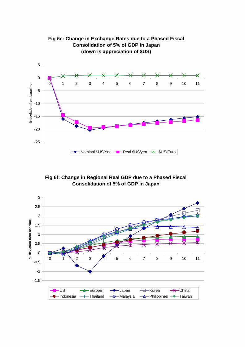
iii) Phased-In Credible Fiscal Consolidation
The new Prime Minister, Mr. Koizumi, has indicated his intention to move toward fiscal
consolidation, committing to limit the budget deficit to 30 trillion Yen in FY2002 and suggesting that
over the medium-term it would be appropriate to eliminate the central government’s primary deficit in
the General Account. At the time of writing this paper, no timeframe had been set for this. In this
simulation, the impact of a phased, fully credible, fiscal consolidation is considered with government
spending reduced by 1.7% of GDP in year one, 3.4% of GDP in year two, and 5.1% of GDP from
��
year 3 onwards (all relative to baseline).4 The results are presented in Figure 6a to 6h. To compare
the difference between phased in fiscal cuts and sharp unannounced cuts the reader only needs to
invert the results in figures 3a to 3g (which were the permanent fiscal spending increase) since both
shocks are scaled to 5% of GDP changes in the long run.
The initial impact of the announcement of fiscal consolidation is to reduce real interest rates and
depreciate the yen by around 15% which leads to a rise in net exports. As households anticipate the
lower future tax obligations they will face, consumption also rises. The rise in consumption and net
exports more than offsets the decline in government expenditure and in private investment, which
declines due to the lower expected growth in the next few years, and real GDP rises. The key point
for growth in the first year is that the financing gains are larger than the fiscal cuts. Given the policy
reaction function, interest rates spike upwards in response to the large depreciation of the yen. If the
BoJ did not raise interest rates (i.e. imposing simulation 1 in figures 2a to 2h), the initial output
response would be even more positive. However, in the second and third years, the positive impact
from the financing gains is more than offset by the impact of the actual decline in government
expenditure, pushing real GDP below that in the baseline, and it is only from the fifth year that real
GDP again moves above the baseline as the positive impact of the decline in real interest rates and the
real exchange rate on consumption, investment, and net exports is fully felt.
The simulation, when compared to (inverse) of the temporary fiscal expansion considered in the
previous section, shows the potential benefits of announcing a fully credible fiscal consolidation
strategy as against one that is not believed. While even in the case of a credible consolidation there
are short-run costs to output as government demand is withdrawn from the economy, these are partly
mitigated by the positive announcement effect on consumption and investment brought about by the
rise in equity prices, decline in long-term interest rates, and the lower future tax liabilities of
households. In the case of the temporary consolidation, none of these offsetting factors are apparent.
4 While it is unlikely that any consolidation would happen this quickly, for the purposes of the simulations it is useful to have it occurring in a relatively short period of time so that the competing effects of the policy become more clearly visible.
��
The impact on the other Asian economies are similar (but opposite in sign) to the results discussed
earlier for a fiscal expansion in Japan. In the first year, the impact again depends on the relative
importance of trade and financial links. Those with important trade links (such as Malaysia) suffer a
modest decline in real GDP as the depreciation of the yen offsets the rise in demand in Japan, but
countries with high debt levels (such as Indonesia) actual see an increase in real GDP. In the second
year, all the Asian economies are gaining more from lower capital costs than they are losing from a
temporary slowdown in Japan and the weaker yen.
6. Conclusions and Policy Implications
The results presented in this paper highlight a number of important issues in understanding the
impacts of macroeconomic policy in Japan.
Firstly, the proposals for macroeconomic policy outlined by Fukao et al (2001) and others are
strongly supported by the empirical model presented in this paper.
Secondly as Japan moves toward fiscal consolidation over the medium-term, the results give
some grounds for optimism that the economic impact can be limited. While undoubtedly there will be
some short-term negative impact on economic activity from a permanent phased fiscal consolidation,
this would be fairly limited if the announcement were credible--perhaps in the form of an announced
and detailed medium—term strategy—and would be quite quickly replaced by the positive impact on
activity from the decline in long term real interest rates and the rise in equity prices. The negative
short-run impact could also be offset by a more expansionary monetary policy through the central
bank’s purchase of government debt or even better, the announcement of a credible inflation target.
As argued in detail in McKibbin and Callen (2001) this paper also shows that the existence of
financial as well as trade linkages means that the negative effects of the demand contraction in Japan
will be transmitted less negatively to the region, making any fiscal consolidation in Japan less
problematic for the other countries in Asia unless the capital markets linkages are constrained because
of other policy objectives.
The model suggests that a quantitative easing of monetary policy by the BoJ through the
outright purchase of government bonds would stimulate the economy in the short-run, and from a
��
position of insufficient demand would help close the output gap. However despite the relatively
optimistic assessment of the impacts of macroeconomic policy in Japan, a range of other problems
also need to be addressed such as the bank loan problems and structural reforms to the Japanese
economy in order to raise productivity growth back towards pre 1990 levels. The aging of the
Japanese population and the impacts of this on potential growth and fiscal balances5 suggest that
Japanese policymakers need to act sooner rather than later to address the serious economic problems
now facing the Japanese economy.
5 See McKibbin and Nguyen (2001) for some results using a similar framework to the model used in this paper.
��
References Bayoumi T. (1999) “The Morning After: Explaining the Slowdown in Japanese Growth in the 1990s” IMF Working Paper WP/99/13. Boltho A. and J. Corbett (2000) “The Assessment: Japan’s Stagnation – Can Policy Revive the Economy” Oxford Review of Economic Policy, vol 16, no 2, page 1-17.
Callen T. and W. McKibbin (2001) “Policies and Prospects in Japan and the Implications for the Asia Pacific Region” IMF Working Paper WP/01/131. Fukao, M., Hoshi, T. and T. Ito (2001) “What Japan Needs: Unconventional Monetary Policy and Aggressive NPL Write-offs” (mimeo) Hayashi, F. (1982) “Tobin’s Marginal q and Average q: A Neoclassical Interpretation.” Econometrica 50, pp.213-224. Hayashi F. and E. Prescott (2001) “The 1990s in Japan: A lost Decade” paper presented at the Spring 2001 International Forum of Collaboration Projects sponsored by the Economic and Social Research Institute of the Japan Cabinet Office in Tokyo, Japan, March 18-20, 2001. Krugman P. (1998) “Its Baaack: Japan’s Slump and the Return of the Liquidity Trap” Brookings Papers on Economic Activity,2, p 137-205. Lucas, R. E.(1967) "Adjustment Costs and the Theory of Supply." Journal of Political Economy 75(4), pp.321-334 Lucas, Robert (1976) “Econometric Policy Evaluation: A Critique” in Brunner Karl and Alan Meltzer (eds.) The Phillips Curve and Labour Markets, Amsterdam: North-Holland. McKibbin W.J. (1996) “The Macroeconomic Experience of Japan 1990 to 1995: An Empirical Investigation” Brookings Discussion Paper in International Economics #131. http://www.msgpl.com.au/msgpl/download/bdp131.pdf McKibbin (2001) “Documentation of the G-Cubed Asia Pacific Model – version 46n” McKibbin Software Group Pty Ltd, Canberra, Australia. http://www.msgpl.com.au/msgpl/apgcubed46n/index.htm McKibbin W and T. Callen (2001) “The Impact of Japan on the Asia Pacific Region” paper presented at the conference on “Economic Interdependence Shaping Asia-Pacific in the 21st Century” held in Tokyo during March 22-23.
��
McKibbin W. and W. Martin (1998) “The East Asia Crisis: Investigating Causes and Policy Responses” Working Paper in Trade and Development #98/6, Economics Department, Research School of Pacific and Asian Studies, Australian National University and Brookings Discussion Paper in International Economics #142, The Brookings Institution, Washington DC. http://www.brook.edu/views/papers/mckibbin/142.pdf McKibbin W. and J. Nguyen (2001) “The Impact of Demographic Change in Japan: Some Preliminary Results from the MSG3 Model” paper presented to the Fall 2001 International Forum of Collaboration Projects, Economic and Social Research Institute of the Japanese Cabinet Office, Tokyo Sept 17-19.
McKibbin W. and A. Stoeckel (1999) “East Asia’s Response to the Crisis: A Quantitative Analysis”, paper prepared for the ASEM Regional Economist’s Workshop: “From Recovery to Sustainable Development” The World Bank. Brookings Discussion Paper in International Economics #149, The Brookings Institution, Washington DC. http://www.msgpl.com.au/msgpl/download/eastasiafinal.PDF McKibbin W.J. and J. Sachs (1991) Global Linkages: Macroeconomic Interdependence and Cooperation in the World Economy, Brookings Institution, June. McKibbin W.J. and D. Vines (2001) “Modelling Reality: The Need for Both Intertemporal Optimization and Stickiness in Models for Policymaking” Oxford Review of Economic Policy vol 16, no 4. (draft version http://www.msgpl.com.au/msgpl/download/McKibbinandVines11.pdf ) McKibbin W. and P. Wilcoxen (1998) “The Theoretical and Empirical Structure of the G-Cubed Model” Economic Modelling , 16, 1, pp 123-148 (ISSN 0264-9993) (working paper version: http://www.msgpl.com.au/msgpl/download/struct.pdf ) Motonishi T and H. Yoshikawa (1999) “Causes of the Long Stagnation of Japan during the 1990s: Financial or Real” Journal of the Japanese and International Economies, 13(4), pp 181-200. Posen A. (1998) “Restoring Japan’s Economic Growth”, Institute for International Economics, Washington DC. Sakakibara, E. and N. Yoshino (2001) “Understanding Recent Slow Growth in Japan: The Way Forward” paper presented at the Harvard University Asian Economic Panel, Cambridge Mass, April 26-27. Treadway, A. (1969) "On Rational Entrepreneurial Behavior and the Demand for Investment." Review of Economic Studies 36(106), pp.227-239. Yoshikawa H. (2000) “Technical Progress and the Growth of the Japanese Economy – Past
��
and Future” Oxford Review of Economic Policy, vol 16, no 2, page 34-45. Wilson D. ((2000) “Japan’s Slowdown: Monetary versus Real Explanations” Oxford Review of Economic Policy, vol 16, no 2, page 18-33.
19
Appendix I: A stylized 2 country G-Cubed model
In this section a stylized 2 country model is presented which distills the essence of the G-
Cubed model and in particular how the intertemporal aspects of the model are handled. The reader
is referred to chapters 2 and 5 of McKibbin and Wilcoxen (2001) for greater detail.
In this stylized model there are 2 symmetric countries (based essentially on US data adjusted
to create symmetry). Each country consists of several economic agents: households, the
government, the financial sector and 2 firms, one each in the 2 production sectors. The two sectors
of production are energy and non-energy (this is much like the aggregate structure of the MSG2
model). The following gives an overview of the theoretical structure of the model by describing the
decisions facing these agents in one of these countries. Throughout the discussion all quantity
variables will be normalized by the economy's endowment of effective labor units. Thus, the
model's long run steady state will represent an economy in a balanced growth equilibrium.
Firms
We assume that each of the two sectors can be represented by a price-taking firm which
chooses variable inputs and its level of investment in order to maximize its stock market value.
Each firm’s production technology is represented by a constant elasticity of substitution (CES)
function. Output is a function of capital, labor, energy and materials:
(1) ( )
−−
∑oi
oi
oi
oi
oi
ijoij
me,l,k,=j
oii x A = Q
σσσσσ
δ /)1(/1)1/(
where Qi is the output of industry i, xij is industry i 's use of input j, and Aio, o
ijδ , and σio are
parameters. Aio reflects the level of technology, σi
o is the elasticity of substitution, and the oijδ
parameters reflect the weights of different inputs in production; the superscript o indicates that the
parameters apply to the top, or “output”, tier. Without loss of generality, we constrain theoijδ 's to
sum to one.
20 The goods and services purchased by firms are, in turn, aggregates of imported and
domestic commodities which are taken to be imperfect substitutes. We assume that all agents in the
economy have identical preferences over foreign and domestic varieties of each commodity. We
represent these preferences by defining composite commodities that are produced from imported
and domestic goods. Each of these commodities, Yi, is a CES function of inputs domestic output,
Qi, and an aggregate of goods imported from all of the country’s trading partners, Mi:
(2) ( ) ( ))1/(
/)1(/1/)1(/1−
−−
+
fdi
fdifd
ifd
ifd
ifd
ifd
ifd
ii
fdifi
fdid
fdii MQ A = y
σσσσσσσσ
δδ
where σifd is the elasticity of substitution between domestic and foreign goods.1 For example, the
energy product purchased by agents in the model are a composite of imported and domestic energy.
The aggregate imported good, Mi, is itself a CES composite of imports from individual countries,
Mic, where c is an index indicating the country of origin:
(3) ( ))1/(
7
1
/)1(/1−
=
−
∑
ffi
ffifd
iff
iff
i
cic
ffic
ffii M A = M
σσσσσ
δ
The elasticity of substitution between imports from different countries is σiff.
By constraining all agents in the model to have the same preferences over the origin of
goods we require that, for example, the agricultural and service sectors have the identical
preferences over domestic oil and imported oil.2 This accords with the input-output data we use
and allows a very convenient nesting of production, investment and consumption decisions.
In each sector the capital stock changes according to the rate of fixed capital formation (Ji)
and the rate of geometric depreciation (/i):
(4) k J = k iiii δ−�
1 This approach follows Armington (1969). 2 This does not require that both sectors purchase the same amount of oil, or even that they purchase oil at all; only that they both feel the same way about the origins of oil they buy.
21 Following the cost of adjustment models of Lucas (1967), Treadway (1969) and Uzawa
(1969) we assume that the investment process is subject to rising marginal costs of installation. To
formalize this we adopt Uzawa's approach by assuming that in order to install J units of capital a
firm must buy a larger quantity, I, that depends on its rate of investment (J/k):
(5) J k
J+ = I i
i
iii
2
1φ
where φi is a non-negative parameter. The difference between J and I may be interpreted various
ways; we will view it as installation services provided by the capital-goods vendor. Differences in
the sector-specificity of capital in different industries will lead to differences in the value of φi.
The goal of each firm is to choose its investment and inputs of labor, materials and energy to
maximize intertemporal net-of-tax profits. For analytical tractability, we assume that this problem
is deterministic (equivalently, the firm could be assumed to believe its estimates of future variables
with subjective certainty). Thus, the firm will maximize:3
(6) dse Ip tsn) sRi
I4i
t
)()(())1(( −−−∞
−−∫ τπ
where all variables are implicitly subscripted by time. The firm’s profits, π, are given by:
(7) ))(1( xpxpxwQp = immiie
eiilii
*i2i −−−−τπ
ZKHUH 22 LV WKH FRUSRUDWH LQFRPH WD[� 24 is an investment tax credit, and p* is the producer price of
the firm’s output. R(s) is the long-term interest rate between periods t and s:
(8) dvvr ts
= sRs
t
)(1
)( ∫−
Because all real variables are normalized by the economy's endowment of effective labor units,
profits are discounted adjusting for the rate of growth of population plus productivity growth, n.
3 The rate of growth of the economy's endowment of effective labor units, n, appears in the discount factor because the quantity and value variables in the model have been scaled by the number of effective labor units. These variables must be multiplied by exp(nt) to convert them back to their original form.
22 Solving the top tier optimization problem gives the following equations characterizing the firm’s
behavior:
(9) ( ) m}e,{l,jp
pQAx
oio
i
j
ii
oi
oijij ∈
=
−σ
σδ
*1
(10) p k
J = I
4i
iii )1)(1( τφλ −+
(11) 2
*
2)1()1()(
−−−−
i
iiI4
i
ii2ii
i
k
Jp
dk
dQp +r =
dsd φ
ττλδλ
where �i is the shadow value of an additional unit of investment in industry i.
Equation (9) gives the firm’s factor demands for labor, energy and materials and equations
(10) and (11) describe the optimal evolution of the capital stock. Integrating (11) along the
optimum trajectory of investment and capital accumulation, ))(ˆ),(ˆ( tktJ , gives the following
expression for �i:
(12) ∫∞
−+−
−+−=
t
tssR
i
iiI
kJi
iii dse
k
Jp
dk
dQpt ))()((
2
4ˆ,ˆ
*2 ˆ
ˆ
2)1()1()( δφ
ττλ
Thus, λi is equal to the present value of the after-tax marginal product of capital in production (the
first term in the integral) plus the savings in subsequent adjustment costs it generates. It is related to
q, the after-tax marginal version of Tobin's Q (Abel, 1979), as follows:
(13) ( ) p
= qI
ii
41 τλ
−
Thus we can rewrite (10) as:
(14) ( )11 −q =
kJ
iii
i
φ
23 Inserting this into (5) gives total purchases of new capital goods:
(15) ( ) iii
i kqI 12
1 2 −=φ
Based on Hayashi (1979), who showed that actual investment seems to be party driven by
cash flows, we modify (15) by writing Ii as a function not only of q, but also of the firm's current
cash flow at time t, πi, adjusted for the investment tax credit:
(16) ( ) ( )( ) I
iii
ii
pkqI
42
22
111
2
1
τ
πα
φα
−−+−=
This improves the model’s ability to mimic historical data and is consistent with the existence of
firms that are unable to borrow and therefore invest purely out of retained earnings.
So far we have described the demand for investment goods by each sector. Investment
goods are supplied, in turn, by a third industry that combines labor and the outputs of other
industries to produce raw capital goods. We assume that this firm faces an optimization problem
identical to those of the other two industries: it has a nested CES production function, uses inputs of
capital, labor, energy and materials in the top tier, incurs adjustment costs when changing its capital
stock, and earns zero profits. The key difference between it and the other sectors is that we use the
investment column of the input-output table to estimate its production parameters.
Households
Households have three distinct activities in the model: they supply labor, they save, and they
consume goods and services. Within each region we assume household behavior can be modeled by
a representative agent with an intertemporal utility function of the form:
(17) dsesg +sc = U t-s-
tt
)())(ln)((ln θ∫∞
where c(s) is the household's aggregate consumption of goods and services at time s, g(s) is
government consumption at s� ZKLFK ZH WDNH WR EH D PHDVXUH RI SXEOLF JRRGV SURYLGHG� DQG � LV WKH
24 rate of time preference.4 The household maximizes (17) subject to the constraint that the
present value of consumption be equal to the sum of human wealth, H, and initial financial assets,
F:5
(18) ttt
tsnsRc FHescsp +=∫∞
−−− ))()(()()(
Human wealth is defined as the expected present value of the future stream of after-tax labor
income plus transfers:
(19) ( ) dseTRL+L+L+LW- = H tsnsR
i
iICG
t
t)()(
12
11 ))()(1( −−−
=
∞
+∑∫ τ
where τ1 is the tax rate on labor income, TR is the level of government transfers, LC is the quantity
of labor used directly in final consumption, LI is labor used in producing the investment good, LG is
government employment, and Li is employment in sector i. Financial wealth is the sum of real
money balances, MON/P, real government bonds in the hand of the public, B, net holding of claims
against foreign residents, A, the value of capital in each sector:
(20) kq+kq+kq+A+B+p
MON = F ii
=i
ccII ∑12
1
Solving this maximization problem gives the familiar result that aggregate consumption
spending is equal to a constant proportion of private wealth, where private wealth is defined as
financial wealth plus human wealth:
(21) )( H+F = cpc θ
However, based on the evidence cited by Campbell and Mankiw (1990) and Hayashi (1982) we
assume some consumers are liquidity-FRQVWUDLQHG DQG FRQVXPH D IL[HG IUDFWLRQ � RI WKHLU DIWHU-tax
4 This specification imposes the restriction that household decisions on the allocations of expenditure among different goods at different points in time be separable. 5 As before, n appears in (18) because the model's scaled variables must be converted back to their original basis.
25 income (INC).6 Denoting the share of consumers who are not constrained and choose
consumption in accordance with (21) by α8, total consumption expenditure is given by:
(22) INC + H+F= cp ttc γαθα )1()( 88 −
The share of households consuming a fixed fraction of their income could also be interpreted as
permanent income behavior in which household expectations about income are myopic.
Once the level of overall consumption has been determined, spending is allocated among
goods and services according to a CES utility function.7 The demand equations for capital, labor,
energy and materials can be shown to be:
(23) { }melkip
pyxp
oc
i
cci
cii ,,,,
1
∈
=
−σ
δ
where y is total expenditure, xic is household demand for good i, σc
o is the top-tier elasticity of
substitution and the δic are the input-specific parameters of the utility function. The price index for
consumption, pc, is given by:
(24) 1
1
,,,
1 −
=
−
= ∑
oco
c
melkjj
cj
c ppσσδ
Household capital services consist of the service flows of consumer durables plus residential
housing. The supply of household capital services is determined by consumers themselves who
invest in household capital, kc, in order to generate a desired flow of capital services, ck, according
to the following production function:
6 There has been considerable debate about the empirical validity of the permanent income hypothesis. In addition the work of Campbell , Mankiw and Hayashi, other key papers include Hall (1978), and Flavin (1981). One side effect of this specification is that it prevents us from computing equivalent variation. Since the behavior of some of the households is inconsistent with (21), either because the households are at corner solutions or for some other reason, aggregate behavior is inconsistent with the expenditure function derived from our utility function. 7 The use of the CES function has the undesirable effect of imposing unitary income elasticities, a restriction usually rejected by data. An alternative would be to replace this specification with one derived from the linear expenditure system.
26
(25) ck k = c α
where α is a constant. Accumulation of household capital is subject to the condition:
(26) k J =k cccc δ−�
We assume that changing the household capital stock is subject to adjustment costs so household
spending on investment, Ic, is related to Jc by:
(27) Jk
J2
+ 1 = I cc
ccc
φ
Thus the household's investment decision is to choose IC to maximize:
(28) ∫∞
−−−−t
tsnsRcIcck dseIpkp ))()(()( α
where pck is the imputed rental price of household capital. This problem is nearly identical to the
investment problem faced by firms and the results are very similar. The only important differences
are that no variable factors are used in producing household capital services and there is no
investment tax credit for household capital. Given these differences, the marginal value of a unit of
household capital, λC, can be shown to be:
(29) ∫∞
−+−
+=
t
tssR
c
ccIckc dse
k
Jppt ))()((
2
ˆ
ˆ
2)( δφαλ
where the integration is done along the optimal path of investment and capital accumulation,
))(ˆ),(ˆ( tktJ cc . Marginal q is:
(30) p
= qIc
cλ
and investment is given by:
27
(31) ( )11 −q =
kJ c
cc
c
φ
The Labor Market
We assume that labor is perfectly mobile among sectors within each region but is immobile
between regions. Thus, wages will be equal across sectors within each region, but will generally
not be equal between regions. In the long run, labor supply is completely inelastic and is determined
by the exogenous rate of population growth. Long run wages adjust to move each region to full
employment. In the short run, however, nominal wages are assumed to adjust slowly according to
an overlapping contracts model where wages are set based on current and expected inflation and on
labor demand relative to labor supply. The equation below shows how wages in the next period
depend on current wages; the current, lagged and expected values of the consumer price level; and
the ratio of current employment to full employment:
(32) 6
55 1
1
11
ααα
=
−
−
++ L
L
p
p
p
pww t
ct
ct
ct
ct
tt
The weight that wage contracts attach to expected changes in the price level is α5 while the weight
assigned to departures from full employment (L ) is α6. Equation (32) can lead to short-run
unemployment if unexpected shocks cause the real wage to be too high to clear the labor market.
At the same time, employment can temporarily exceed its long run level if unexpected events cause
the real wage to be below its long run equilibrium.
The Government
We take each region's real government spending on goods and services to be exogenous and
assume that it is allocated among inputs in fixed proportions, which we set to 1996 values. Total
government outlays include purchases of goods and services plus interest payments on government
debt, investment tax credits and transfers to households. Government revenue comes from sales
taxes, corporate and personal income taxes, and from sales of new government bonds. In addition,
28 there can be taxes on externalities such as carbon dioxide emissions. The government
budget constraint may be written in terms of the accumulation of public debt as follows:
(33) ttttttt TTRGBrDB −++==�
where B is the stock of debt, D is the budget deficit, G is total government spending on goods and
services, TR is transfer payments to households, and T is total tax revenue net of any investment tax
credit.
We assume that agents will not hold government bonds unless they expect the bonds to be
paid off eventually and accordingly impose the following transversality condition:
(34) ( ) 0)(lim )( = esB snsR
s
−−
∞→
This prevents per capita government debt from growing faster than the interest rate forever. If the
government is fully leveraged at all times, (34) allows (33) to be integrated to give:
(35) ( )dseTRGTB tsnsR
tt
−−−∞
−−= ∫ ))(()(
Thus, the current level of debt will always be exactly equal to the present value of future budget
surpluses.8
The implication of (35) is that a government running a budget deficit today must run an
appropriate budget surplus as some point in the future. Otherwise, the government would be unable
to pay interest on the debt and agents would not be willing to hold it. To ensure that (35) holds at
all points in time we assume that the government levies a lump sum tax in each period equal to the
value of interest payments on the outstanding debt.9 In effect, therefore, any increase in government
debt is financed by consols, and future taxes are raised enough to accommodate the increased
interest costs. Other fiscal closure rules are possible, such as requiring the ratio of government debt
8 Strictly speaking, public debt must be less than or equal to the present value of future budget surpluses. For tractability we assume that the government is initially fully leveraged so that this constraint holds with equality. 9 In the model the tax is actually levied on the difference between interest payments on the debt and what interest payments would have been if the debt had remained at its base case level. The remainder, interest payments on the base case debt, is financed by ordinary taxes.
29 to GDP to be unchanged in the long run. These closures have interesting implications but are
beyond the scope of this paper.
Financial Markets and the Balance of Payments
The eight regions in the model are linked by flows of goods and assets. Flows of goods are
determined by the import demands described above. These demands can be summarized in a set of
bilateral trade matrices which give the flows of each good between exporting and importing
countries.
Trade imbalances are financed by flows of assets between countries. Each region with a
current account deficit will have a matching capital account surplus, and vice versa.10 We assume
asset markets are perfectly integrated across regions.11 With free mobility of capital, expected
returns on loans denominated in the currencies of the various regions must be equalized period to
period according to a set of interest arbitrage relations of the following form:
(36) E
E + i =i j
k
jk
jjkk
�
µµ ++
where ik and i j are the interest rates in countries k and j, µk and µj are exogenous risk premiums
demanded by investors (calibrated in the baseline to make the model condition hold exactly with
actual data), and Ekj is the exchange rate between the currencies of the two countries.
Capital flows may take the form of portfolio investment or direct investment but we assume
these are perfectly substitutable ex ante, adjusting to the expected rates of return across economies
and across sectors. Within each economy, the expected returns to each type of asset are equated by
arbitrage, taking into account the costs of adjusting physical capital stock and allowing for
exogenous risk premiums. However, because physical capital is costly to adjust, any inflow of
financial capital that is invested in physical capital will also be costly to shift once it is in place.
10 Global net flows of private capital are constrained to be zero at all times – the total of all funds borrowed exactly equals the total funds lent. As a theoretical matter this may seem obvious, but it is often violated in international financial data. 11 The mobility of international capital is a subject of considerable debate; see Gordon and Bovenberg (1994) or Feldstein and Horioka (1980).
30 This means that unexpected events can cause windfall gains and losses to owners of physical
capital and ex post returns can vary substantially across countries and sectors. For example, if a
shock lowers profits in a particular industry, the physical capital stock in the sector will initially be
unchanged but its financial value will drop immediately.
Money Demand
Finally, we assume that money enters the model via a constraint on transactions.12 We use a
money demand function in which the demand for real money balances is a function of the value of
aggregate output and short-term nominal interest rates:
(37) iPY = MON ε
where Y is aggregate output, P is a price index for Y, i LV WKH LQWHUHVW UDWH� DQG 0 LV WKH LQWHUHVW
elasticity of money demand. The supply of money is determined by the balance sheet of the central
bank and is exogenous.
Assessing the Model All models have strengths and weaknesses and G-Cubed is no exception. Its most important
strength is that it distinguishes between financial and physical capital and includes a fully integrated
treatment of intertemporal optimization by households, firms and international portfolio holders.
This allows the model to do a rigorous job of determining where physical capital ends up, both
across industries and across countries, and of determining who owns the physical capital and in
what currency it is valued. Overall, the key feature of G-Cubed is its treatment of capital, and that
is also what most distinguishes it from other models in either the macro, trade or CGE literatures.
G-Cubed also has other strengths. All budget constraints are satisfied at all times, including
both static and intertemporal budget constraints on households, governments and countries. Short-
run behavior captures the effects of slow wage adjustment and liquidity constraints, while long-run
behavior is consistent with full optimization and rational expectations. In addition, wherever
12 Unlike other components of the model we simply assume this rather than deriving it from optimizing behavior. Money demand can be derived from optimization under various assumptions: money gives direct utility; it is a factor of production; or it must be used to conduct transactions. The distinctions are unimportant for our purposes.
31 possible the model’s behavioral parameters are determined by estimation, which is discussed
further in Chapter 4 of McKibbin and Wilcoxen (2001).
Table 1: A Comparison of Global Dynamic Intertemporal GE models MSG2 G-Cubed G-Cubed (Asia Pacific) Countries: United States United States United States Japan Japan Japan Canada Canada Australia Germany New Zealand New Zealand United Kingdom Australia Korea France Rest of OECD Rest of OECD Italy China China Austria EEFSU India Australia OPEC Thailand Mexico Rest of World Malaysia Korea Singapore High Income Asia Indonesia Low Income Asia Hong Kong Rest of the EMS Taiwan Rest of the OECD Philippines OPEC OPEC EEFSU EEFSU Rest of World Rest of World
Sectors:
Single sector Electric Utilities Energy Gas Utilities Petroleum Refining Coal Mining Crude Oil & Gas Extraction Other Mining Mining Agriculture, Fishing Agriculture Forestry & wood products Durable Manufacturing Durable Manufacturing Non-Durable Manufacturing Non-Durable Manufacturing Transportation Services Services
M:\PAPERS\IMF2001\Paper_Fig1(1).Doc May 17, 2001 (3:30 PM)